Scholte Wave Dispersion Modeling and Subsequent Application in Seabed Shear-Wave Velocity Profile Inversion

Abstract

Recent studies have illustrated that the Multichannel Analysis of Surface Waves (MASW) method is an effective geoacoustic parameter inversion tool. This particular tool employs the dispersion property of broadband Scholte-type surface wave signals, which propagate along the interface between the sea water and seafloor. It is of critical importance to establish the theoretical Scholte wave dispersion curve computation model. In this typical study, the stiffness matrix method is introduced to compute the phase speed of the Scholte wave in a layered ocean environment with an elastic bottom. By computing the phase velocity in environments with a typical complexly varying seabed, it is observed that the coupling phenomenon occurs among Scholte waves corresponding to the fundamental mode and the first higher-order mode for the model with a low shear-velocity layer. Afterwards, few differences are highlighted, which should be taken into consideration while applying the MASW method in the seabed. Finally, based on the ingeniously developed nonlinear Bayesian inversion theory, the seafloor shear wave velocity profile in the southern Yellow Sea of China is inverted by employing multi-order Scholte wave dispersion curves. These inversion results illustrate that the shear wave speed is below 700 m/s in the upper layers of bottom sediments. Due to the alternation of argillaceous layers and sandy layers in the experimental area, there are several low-shear-wave-velocity layers in the inversion profile.

1. Introduction

The MASW method was initially developed as an inversion method in order to map the near-surface of Earth’s structure, by recording and analyzing dispersion of Rayleigh-type surface waves. The method requires an accurately recorded Rayleigh wavefield to be analyzed for its dispersive properties. In addition, the method involves the inversion of the dispersion curve to be performed in order to yield the site properties capable of controlling the observed Rayleigh wave dispersion, i.e., mainly the shear wave velocity profile.

Contemporary studies have exhibited that the MASW method is an effective geoacoustic parameter inversion tool, which employs the dispersion curve of Scholte-type surface waves on the seafloor [1,2,3,4,5,6]. The applicable methodology of underwater MASW is explicitly illustrated in Figure 1. However, in contrast, a negligible amount of work on theoretical modeling of Scholte wave dispersion curves has been reported to date. Due to the varying excitation circumstances of the Rayleigh wave and Scholte wave, Rayleigh waves propagate along the free surface of a solid medium, whereas Scholte waves propagate at the fluid/solid interface. Although there are many methods for computing the dispersion curve of the Rayleigh wave, they are not suitable for Scholte wave simulation. In this regard, it is necessary to establish the theoretical Scholte wave dispersion simulation model.

The computation of the surface wave dispersion curve not only serves for inversion, but also is the primary step of simulating the guided wave fields. The Thomson–Haskell matrix method [7,8] is an efficient method for dispersion curve computation at low frequencies. However, due to the exponentially rising term in the Thomson–Haskell matrix, the method is unstable at a relatively high frequency. In order to overcome the obstacle of a high frequency numerical value, varying attempts have been made in the literature [9,10,11]. Another common method for computing the dispersion curve is the reflection and transmission matrix method, which was proposed by Kennett [12,13]. Based on the dispersion forward model developed over the years, the dispersion characteristics of multi-order surface waves in complex environments are studied, which lays a foundation for its engineering application [14,15,16].

The stiffness matrix method is a relatively mature method to simulate the propagation of waves in layered media. It has been successfully applied to various problems [17,18,19,20] during the most recent few decades. The stiffness matrix method conjoins the displacements and stresses on both sides of the interface via the so-called stiffness matrix. The stiffness matrix is endowed with novel physical meaning, but its idea is analogous to the reflection and transmission matrix method. The stiffness matrix method has some characteristics as well as improvements, which can encourage the employment of the method in theory as well as in certain applications. Some of such characteristics are introduced and discussed in this particular study, including: (a) the forms of water layer stiffness matrices capable of analyzing fluid-elastic-coupled models; (b) the stiffness matrix of a vertically transverse isotropic elastic layer.

The shear wave velocity profile of the seafloor not only provides an important indicator for sedimentary rigidity, but also plays an important role in sedimentary characteristics, seismic detection, and assessment of earth hazards [21]. Furthermore, the variation of shear wave velocities provides an important mechanism for ocean acoustic propagation loss in environments with low shear velocities. This particular mechanism may be regarded as a major factor to be considered in establishing acoustic propagation models as well as in predicting sonar performance [22]. It is an efficient and convenient method to estimate the velocity gradient of the shearing wave in the seabed by inverting the dispersion curve of the seawater–seabed interface wave [6,23]. In recent years, Bayesian inversion methods have made great progress and played an important role in estimating seabed properties and uncertainties based on Bayesian formulas [24,25]. It can estimate the parameters of the maximum posteriori probability (MAP) model effectively, and then analyze the uncertainty of the inversion results qualitatively and quantitatively from the perspective of statistics. In our inversion work, high quality multi-channel seismic data are processed and good Scholte wave dispersion curves are obtained. Our Bayesian inversion produces unexpected new results. Previous inversion results of s-wave velocity profiles show that the s-wave velocity increases with the increase of depth. We found that under Jiao Lai basin sedimentary can be divided into argillaceous layers (clayey silt and silty sand) and the sand layer, two kinds of sediment appear alternately, caused the frequent alternation of high speed and low speed layer.

In the ensuing sections of the manuscript, we present the theoretical formulas of the stiffness matrix method and their root-searching schemes. In addition, the stability of the stiffness matrix method is analyzed. Similarly, the anomalies among the Rayleigh-type surface wave and Scholte type surface wave are illustrated. Furthermore, the impact of dispersion curves due to a vertically transverse isotropic layer is discussed. Finally, the fundamental and first higher-order mode Scholte waves excited by a large-volume air gun array near the sea surface are obtained by employing multi-channel seismic records. Similarly, ocean bottom shear wave profiles are obtained by phase velocity inversion.

2. Brief Description of Theory

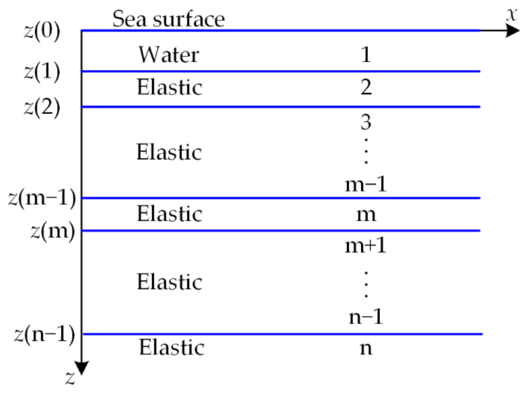
2.1. Scholte Wave Dispersion Modeling

The stiffness matrix method is employed in this particular study to directly relate the forces at the layer interface to the displacements at the same position. The horizontal layered solid medium model is considered in this study, whose surface layer is a liquid layer, which can actually simulate the stratified marine earth model, as depicted in Figure 2. Considering a plane wave propagating in the model, the x-axis represents the wave propagation direction along the sea surface, whereas the z-axis is computed as a positive downward into the medium.

In order to express the stiffness matrix of the elastic medium from the second layer to the (n − 1)th layer, the reference [17] has derived it in detail. The external load vector on the upper and lower interfaces of the mth layer are expressed by the displacements at the interfaces as:

$$\left[\begin{array}{c}{p}_m(z_{m-1})\\ p_m(z_m)\end{array}\right]=\left[\begin{array}{cc}{K}_{11}^m& K_{12}^m\\ K_{21}^m& K_{22}^m\end{array}\right]\left[\begin{array}{c}{d}_m(z_{m-1})\\ d_m(z_m)\end{array}\right],$$

(1)

or briefly,

$$P_m=K^m{D}_m,$$

(2)

where $K^m$ is the stiffness matrix of the layer with $2\times 2$ submatrix $K_{ij}^m$; $P_m={\left[\begin{array}{cccc}{\sigma }_m(z_m)& {\tau }_m(z_m)& -{\sigma }_m(z_{m-1})& -{\tau }_m(z_{m-1})\end{array}\right]}^T$ is the external load vector, the symbols $\sigma$ and $\tau$ represent the normal and shear stresses at the interface, respectively; and $D_m={\left[\begin{array}{cccc}{u}_m(z_{m-1})& w_m(z_{m-1})& u_m(z_m)& w_m(z_m)\end{array}\right]}^T$ is the displacement vector, the symbols $u$ and $w$ represent the horizontal and vertical displacements at the interface, respectively. It can be illustrated that $K^m$ is symmetric.

For the half-space layer, which satisfies the infinite radiation condition, there is no upward propagating wave. The relationship among potential functions, displacements, and stresses at the upper interface is:

$$\left[\begin{array}{c}{u}_n(z_{n-1})\\ w_n(z_{n-1})\\ {\sigma }_n(z_{n-1})\\ {\tau }_n(z_{n-1})\end{array}\right]=\left[\begin{array}{cccc}-ik& -i{\beta }_n& ik& i{\beta }_n\\ -i{\alpha }_n& -ik& i{\alpha }_n& -ik\\ {\mu }_n{a}_n& 2i{\mu }_{n}k{\beta }_n& {\mu }_n{a}_n& -2i{\mu }_{n}k{\beta }_n\\ -2i{\mu }_{n}k{\alpha }_n& {\mu }_n{a}_n& 2i{\mu }_{n}k{\alpha }_n& {\mu }_n{a}_n\end{array}\right]\left[\begin{array}{c}0\\ 0\\ {\phi }_n^D(z_{n-1})\\ {\psi }_n^D(z_{n-1})\end{array}\right],$$

(3)

where $a_m=2k^2-{\omega }^2/\left(c_{sm}^2\right)$; ${\alpha }_n=\frac{\omega }{c}\sqrt{1-{\left(c/c_{pn}\right)}^2}$ and ${\beta }_n=\frac{\omega }{c}\sqrt{1-{\left(c/c_{sn}\right)}^2}$ are vertical wavenumbers; ${\mu }_n$ is the Lamé coefficients (${\mu }_1=0$ for the water layer) and ${\phi }_n^D$ is the potential function of the downward propagating wave in the half-space layer. We transformed Equation (3) into the following form:

$$\left[\begin{array}{c}{d}_n(z_{n-1})\\ F_n(z_{n-1})\end{array}\right]=\left[\begin{array}{c}{H}_{12}^n\\ H_{22}^n\end{array}\right]{\Phi }_n(z_{n-1}),$$

(4)

where ${\Phi }_n(z_{n-1})={\left[\begin{array}{cc}{\phi }_n^D(z_{n-1})& {\psi }_n^D(z_{n-1})\end{array}\right]}^T$, $H_{12}^n=\left[\begin{array}{cc}{T}_{13}^n& T_{14}^n\\ T_{23}^n& T_{24}^n\end{array}\right]$, $d_n(z_{n-1})=\left[\begin{array}{c}{u}_n(z_{n-1})\\ w_n(z_{n-1})\end{array}\right]$, $F_n(z_{n-1})=\left[\begin{array}{c}{\sigma }_n(z_{n-1})\\ {\tau }_n(z_{n-1})\end{array}\right]$ and $H_{22}^n=\left[\begin{array}{cc}{T}_{33}^n& T_{34}^n\\ T_{43}^n& T_{44}^n\end{array}\right]$. According to the above equation, the potential function can be expressed as:

$${\Phi }_n(z_{n-1})={\left(H_{12}^n\right)}^{-1}{d}_n(z_{n-1}),$$

(5)

$${\Phi }_n(z_{n-1})={\left(H_{22}^n\right)}^{-1}{F}_n(z_{n-1}),$$

(6)

Then, the stress vector can be expressed by the displacement vector as:

$$F_n(z_{n-1})=H_{22}^n{\left(H_{12}^n\right)}^{-1}{d}_n(z_{n-1}),$$

(7)

Defining the external forces on upper interface $z_{n-1}$ as $p_n(z_{n-1})=F_n(z_{n-1})$, Equation (7) can be expressed in the form of stiffness matrix as in [26]:

$$p_n(z_{n-1})=K^n{d}_n(z_{n-1}),$$

(8)

There is no shear component in the fluid layer, and the displacement of the sea surface and seabed can be expressed by the potential function as:

$$\left[\begin{array}{c}{w}_1(z_0)\\ w_1(z_1)\end{array}\right]=\frac{{\alpha }_1}{\sinh {\alpha }_1{h}_1}\left[\begin{array}{cc}-\cosh {\alpha }_1{h}_1& 1\\ -1& \cosh {\alpha }_1{h}_1\end{array}\right]\left[\begin{array}{c}{\phi }_1(z_0)\\ {\phi }_1(z_1)\end{array}\right],$$

(9)

where $w_1$ is the vertical displacement and ${\phi }_1$ is the velocity potential in water. In the background of the layer stiffness matrix method, we need to consider the volume perturbance as the flux condition at the interface, for example, the injection volume is expressed by the source in the form of the air gun at the interface. We employ a set of constitutive laws of ${\overline{v}}_1(z_0)=-j\omega w_1(z_0)$, ${\overline{v}}_1(z_1)=-j\omega w_1(z_1)$, $p_1(z_0)=-{\sigma }_1(z_0)$ and $p_1(z_1)={\sigma }_1(z_1)$. Then, we acquire the following stiffness matrix [17] as:

$$K^1=\frac{{\rho }_1{\omega }^2}{{\alpha }_1\sinh {\alpha }_1{h}_1}\left[\begin{array}{cc}\cosh {\alpha }_1{h}_1& -1\\ -1& \cosh {\alpha }_1{h}_1\end{array}\right],$$

(10)

The aforementioned stiffness matrices for the water and elastic layers are employed to construct the global stiffness matrix for a layered system. The global stiffness matrix is developed by conjoining the stiffness matrices of Equations (2), (8) and (10) as:

$$K=\left[\begin{array}{cccccccc}{K}_{11}^1& K_{12}^1& 0& 0& 0& 0& 0& 0\\ \begin{array}{c}0\\ K_{21}^1\end{array}& \left[\begin{array}{cc}0& 0\\ 0& K_{22}^1\end{array}\right]+K_{11}^2& K_{12}^2& 0& 0& 0& 0& 0\\ 0& K_{21}^2& K_{22}^2+K_{11}^3& K_{12}^3& 0& 0& 0& 0\\ 0& 0& K_{21}^3& K_{22}^3+K_{11}^4& K_{12}^4& 0& 0& 0\\ 0& 0& 0& \ddots & \ddots & \ddots & 0& 0\\ 0& 0& 0& 0& K_{21}^{n-3}& K_{22}^{n-3}+K_{11}^{n-2}& K_{12}^{n-2}& 0\\ 0& 0& 0& 0& 0& K_{21}^{n-2}& K_{22}^{n-2}+K_{11}^{n-1}& K_{12}^{n-1}\\ 0& 0& 0& 0& 0& 0& K_{21}^{n-1}& K_{22}^{n-1}+K^n\end{array}\right],$$

(11)

The global stiffness matrix for a system comprising of $(n-2)$ elastic layers, with the half-space layer, and overlaid by water, is a $\left(2n-1\right)\times \left(2n-1\right)$ symmetric matrix, which satisfies the following relationship as:

$$p=Kd,$$

(12)

The sea surface free boundary condition is given by:

$$p_0=0,$$

(13)

For any other interface due to the continuity of stress, all elements are equivalent to zero. Thus, the solution for Scholte waves must satisfy $Kd=0$, and the dispersion function is therefore expressed as:

$$\Delta \left(\omega ,k\right)=\left|K\right|=0,$$

(14)

The overall stiffness matrix of the entire system can be combined by employing this particular method. The global load vector corresponds to the external forces at the interface of the layered system. By using the stiffness matrix method, the characteristic equation can be established to determine the mode shapes of the layered system. Thus, the theoretical dispersion curve of the surface wave propagating in the layered system can be ascertained.

2.2. Bayesian Inversion Theory

The solution of the inversion problem is transformed into the solution of parametric posteriori probability density (PPD) based on Bayesian theory in this particular study. Adaptive Simplex Simulated Annealing (ASSA), a nonlinear global optimization algorithm, is used to solve the maximum of a posterior probability (MAP) model, and then a Bayesian information criterion (BIC) is employed to select the model.

The experimentally measured data vector is set as d with element d_i, and m as the model vector composed of the bottom parameters m_i to be retrieved. Both d_i and m_i were random variables, which were correlated by Bayes’ rule [27]

$$P(m\left|d\right.)=P(d\left|m\right.)P(m)/P(d),$$

(15)

where $P(m\left|d\right.)$ is the PPD; $P(m\left|d\right.)$ is the conditional probability density function (PDF) of m under measured data; P(m) is the prior PDF of m, $P(d)$ is the PDF of d. As the $P(d)$ is independent of m, and the $P(d\left|m\right.)$ can be regarded as the likelihood function L(d|m) for the measured data [27], Equation (15) can be written as:

$$P(m\left|d\right.)\propto L(m)P(m),$$

(16)

The likelihood function is ascertained by the form of the data and the statistical distribution of the data errors. Regarding the difficulty of acquiring independent estimation of error statistics in pragmatic applications, the assumption of unbiased Gaussian error is adopted for processing, and the form of the likelihood function is:

$$L(m)=P(d\left|m\right.)\propto \exp [-E(m)],$$

(17)

where $E(m)$ is the cost function. Hence, the $P(m\left|d\right.)$ becomes:

$$P(m\left|d\right.)\propto \exp [-E(m)]P(m),$$

(18)

Normalizing the above equation, we have:

$$P(m\left|d\right.)=\frac{\exp [-E(m)]P(m)}{{\displaystyle \int \exp [-E(m^{\prime })]P(m^{\prime })d{m}^{\prime }}},$$

(19)

The domain of integration spans the M-dimensional parameter space, and the integrated components are distinguished by single quotation marks, where M is the number of parameters waiting for inversion.

In Bayesian theory, the posterior probability density (PPD) of m can be regarded as the inversion outcomes. To interpret the M-dimensional PPD requires estimating properties of the parameter value, uncertainties, and inter-relationships, i.e., the MAP model $\widehat{m}$, mean model $\overline{m}$, model covariance matrix C_m and marginal probability distributions P(m_i|d). These properties are respectively defined as:

$$\widehat{m}={\mathrm{Arg}}_{\max }\{P(m\left|d\right.)\},$$

(20)

$$\overline{m}={\displaystyle \int m^{\prime }P(m^{\prime }|d)d{m}^{\prime }},$$

(21)

$${\mathbf{C}}_m={\displaystyle \int (m^{\prime }-\overline{m^{\prime }})){(m^{\prime }-\overline{m^{\prime }})}^{T}P(m^{\prime }|d)d{m}^{\prime }},$$

(22)

$$P(m_i|d)={\displaystyle \int \delta (m_i-m_i{}^{\prime })P(m^{\prime }|d)d{m}^{\prime }},$$

(23)

where T is the transpose symbol.

3. Dispersion Simulation of Layered Ocean Bottom

Theoretical dispersion curves can be obtained by solving Equation (14). There are four main techniques to ascertain the roots, i.e., the bisection searching technique [28], two dimensional searching technique [29], least absolute determinant [30], and phase-velocity scanning technique [31]. Since the singularity of a stiffness matrix can be better characterized by its minimum absolute eigenvalue, the method of least absolute determinant is employed for this particular study.

3.1. Fundamental Mode Dispersion

The method was analyzed for a number of varying cases, of which a couple are presented here.

Table 1. Parameters of layered ocean Model 1.

Case 1	${\mathit{v}}_{\mathit{p}} \left(\mathbf{m}/\mathbf{s}\right)$	${\mathit{v}}_{\mathit{s}} \left(\mathbf{m}/\mathbf{s}\right)$	$\mathbf{Density}\left(\mathbf{g}/{\mathbf{cm}}^3\right)$	Thickness (m)
Layer 1	1500	-	1.0	100
Layer 2	1800	500	1.5	70
Layer 3	2400	800	1.9	50
Layer 4	2800	1200	2.3	Infinite

illustrates the first model of three layers of an elastic medium covered with a liquid layer. The compressional wave velocity $v_p$, shear wave velocity $v_s$ of elastic medium and the medium density increases with depth. The compressional wave velocity of water is $1500 \mathrm{m}/\mathrm{s}$ and the density is $1.0 \mathrm{g}/{\mathrm{cm}}^3$.

An effort to ascertain the roots of the dispersion function of Model 1 at the frequency of 5, 10 and 20 Hz is conducted. The absolute determinant of stiffness matrix and their roots are illustrated in Figure 3. By comparing the top and bottom panels of Figure 3, the roots of high frequency dispersion function in the phase velocity domain are more similar to those of the low frequency dispersion function. In the bottom panel of Figure 3, the frequency is high, i.e., up to 20 Hz, and no numerical instability is found in the stiffness matrix method. We have computed the dispersion function of the Scholte wave, i.e., up to 50 Hz, and did not observe any numerical instabilities of high frequency. Furthermore, we acquired reliable and stable solutions by testing other models as well.

By solving the dispersion function at the frequency 0.1–50 Hz, the first root at all frequencies constitutes the fundamental mode dispersion curve of the Scholte wave (red solid line in Figure 4a). In order to analyze the influence of the water layer, the fluid layer of Model 1 was removed, then the dispersion curve of the Rayleigh wave was computed (Figure 4a blue circles). At high frequencies, the phase velocities of both types of surface waves do not alter with frequency. The wave velocity is higher for the fundamental mode in case there is no liquid surface, the fundamental mode Scholte wave velocity is 432 m/s, while the Rayleigh wave velocity is 475 m/s. It is evident that regardless of the existence of the liquid layer, the fundamental mode of the dispersion curve of the surface wave has no cut-off frequency.

Subsequently, Model 2, with a low shear-velocity layer, is analyzed. The low shear-velocity layer is defined such that the shear velocity of the layer is lower than that of its overburden layer. The model parameters are exhibited in

Table 2. Parameters of layered ocean Model 2.

Case 2	${\mathit{v}}_{\mathit{p}} \left(\mathbf{m}/\mathbf{s}\right)$	${\mathit{v}}_{\mathit{s}} \left(\mathbf{m}/\mathbf{s}\right)$	$\mathbf{Density}\left(\mathbf{g}/{\mathbf{cm}}^3\right)$	Thickness (m)
Layer 1	1500	-	1.0	20
Layer 2	1800	600	1.5	10
Layer 3	2400	500	1.9	20
Layer 4	2400	800	1.9	30
Layer 5	2800	1200	2.3	Infinite

. The third layer is a low shear-velocity layer with a thickness of 20 m. In addition, Model 2 is different from Model 1 in that its layer thickness is smaller and the medium parameters fluctuate severely. It is pertinent to mention that Model 2 employs the same root search scheme as Model 1.

The red solid line in Figure 4b represents the fundamental mode dispersion curve of Model 2, and the blue circles are the dispersion curve of the Rayleigh wave which is computed by removing the fluid layer of Model 2. By comparing the left and right panels of Figure 2, the dispersion curves of Model 2 exhibit larger phase-velocity perturbations than those of Model 1. The surface wave penetration depth in the elastic medium is roughly one-half of the Scholte wavelength [32]. When the thickness of layers is small, the penetration depth of the Scholte wave in the solid is larger when compared to the thickness of upper layers in the selected frequency band (Figure 5b). Consequently, the phase velocity will be affected by the layered model parameters. For the model with a large layer thickness, the penetration depth of the Scholte wave is smaller than the thickness of the first elastic layer (Figure 5a), and the dispersion curve is close to the case of the semi-infinite seabed. The bending of the dispersion curve of Model 1 requires very low frequency.

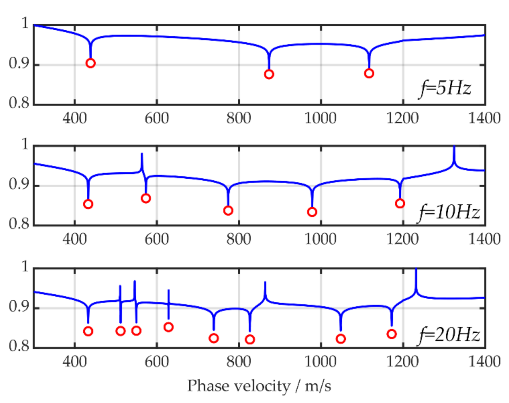
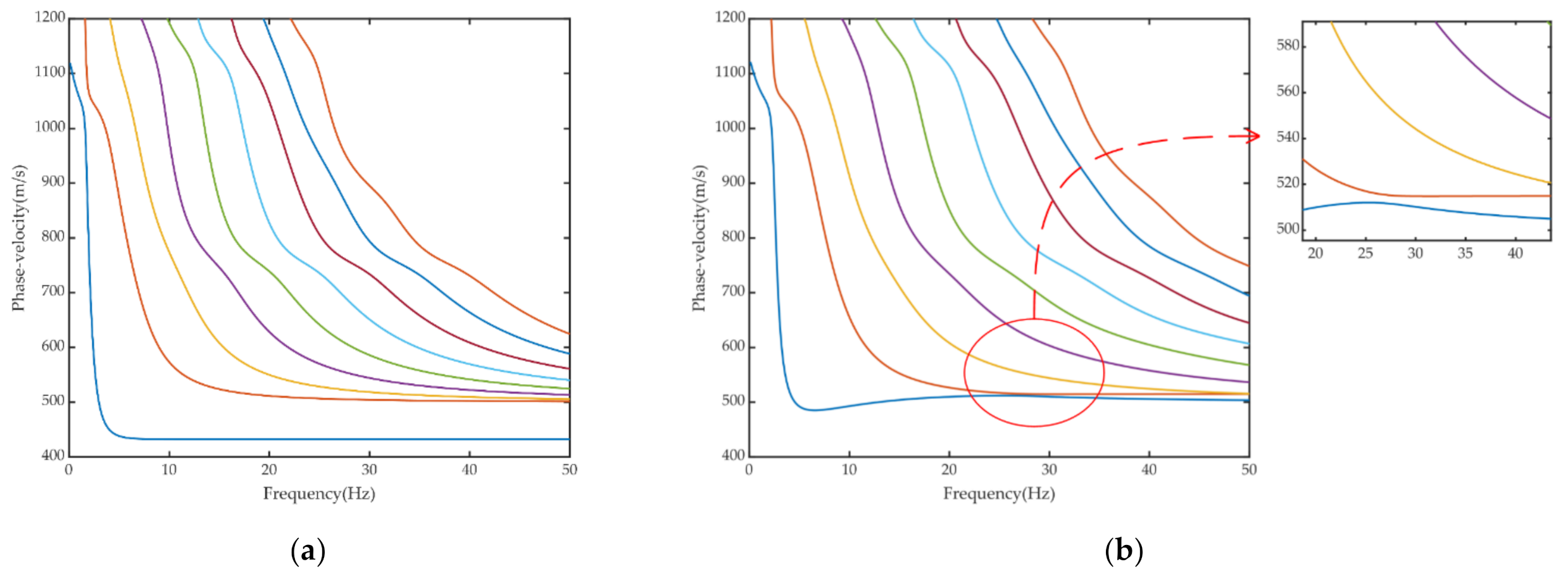
3.2. Fundamental and Higher Mode Dispersion

Figure 6a demonstrates the dispersion curves of the first nine modes, i.e., fundamental mode, as well as eight higher modes of Model 1. Higher-order modes have larger phase-velocity perturbations than the lower-order modes. All the higher modes approach the velocity of 500 m/s at high frequencies, which is the shear wave velocity in the first elastic layer of Model 1.

Figure 6b represents the dispersion curves of the first nine modes, i.e., fundamental mode, as well as eight higher modes of Model 2. Due to the existence of a low shear-velocity layer, the first two mode curves get very close to each other at a frequency range of 25–30 Hz. The zoomed panel in Figure 6b illustrates that there is no point of intersection, and the two curves indeed do not intersect. However, the distance among two curves is negligibly small. Boaga, J. et al. [33] proved that the Rayleigh wave dispersion curve has the same rule when there is a low shear-velocity layer. They titled it, “osculation frequency”, and proved that it exists in strong impedance contrast. Below this frequency, the energy of the vertical component is transferred from the fundamental to the first higher mode. In particular, the consequences of inverting the apparent dispersion curve are severe, and result from the combination of the two modes. Due to this combination, it is erroneously assumed to correspond to the fundamental mode. The errors in terms of depth and velocity of the bedrock can be large, and these parameters are of utmost interest in engineering surveys.

The higher mode dispersion curve in Figure 6a as well as in Figure 6b appear to be more sensitive to the layered model parameters as compared to the fundamental mode. Scholte wave amplitudes decrease exponentially with increasing distance from the interface, so it is confined to a narrow stratum in the proximity of the interface. For higher modes, the horizontal wave number $k=\omega /c_{phase}$. The higher the order, the smaller the incidence angle, and the larger the number of seabed layers are affected, as illustrated in Figure 7. Employing MASW for the inversion of ocean bottom parameters, including higher order modes, offers additional information leading to higher resolution and smaller uncertainties.

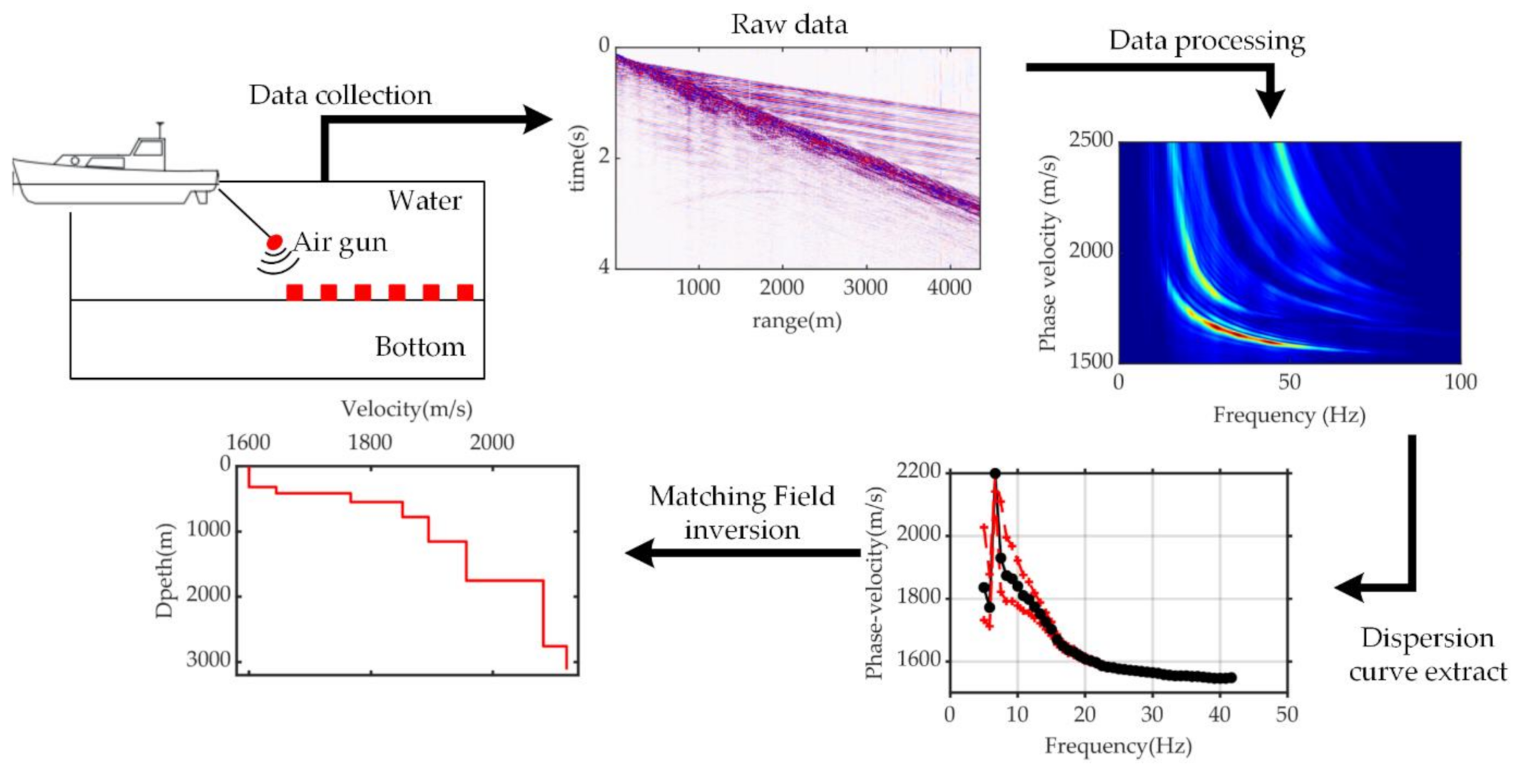
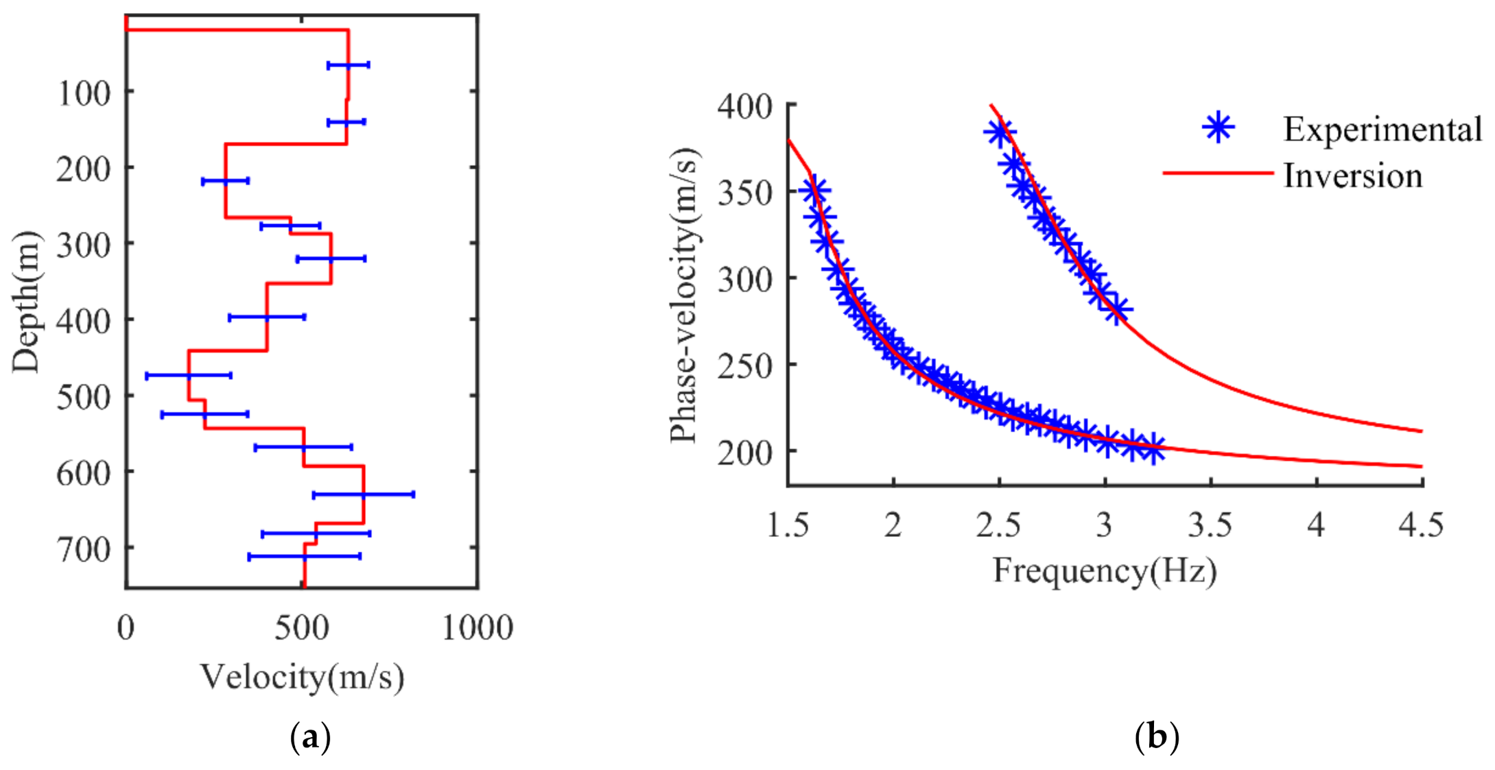
4. Geoacoustic Inversion with Experimental Data

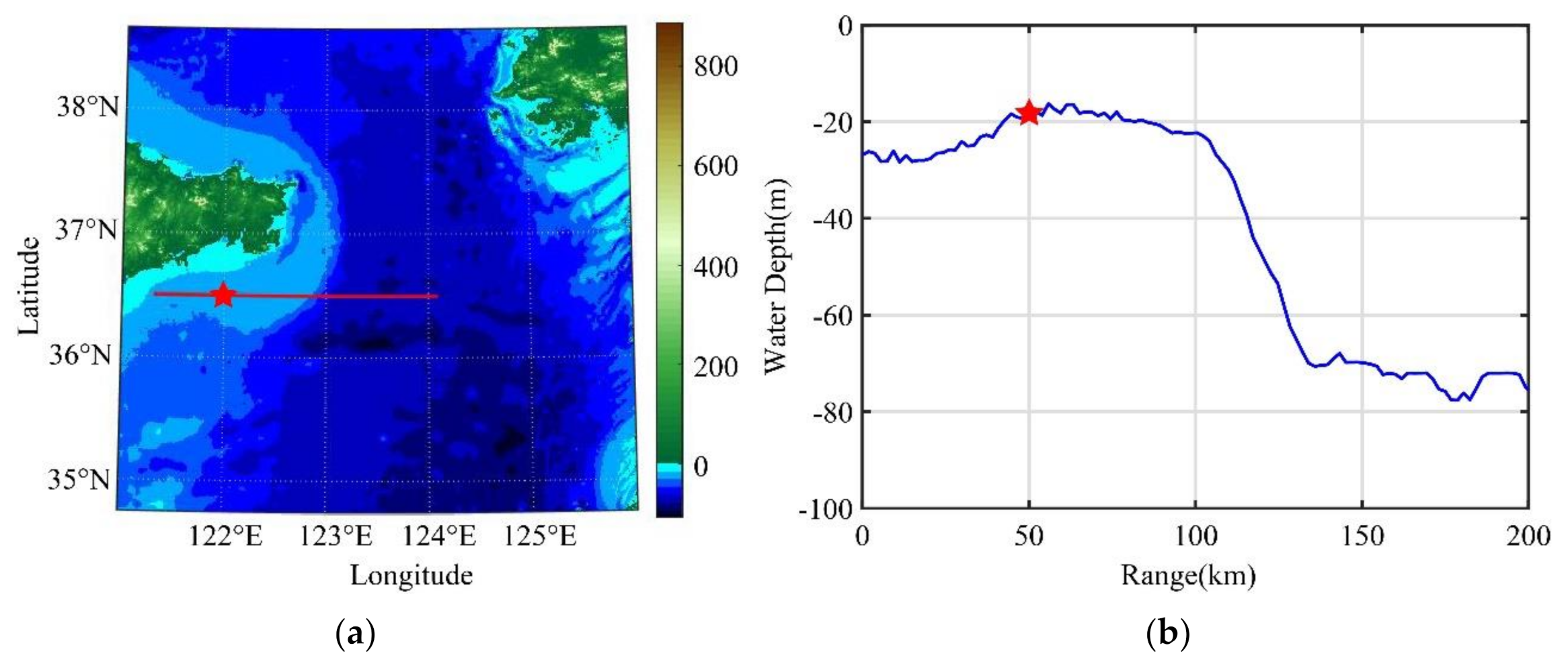
4.1. Experimental Configuration and Data Description

The multi-channel seismic exploration experiment was carried out in the southern Yellow Sea of China. The experimental area is exhibited in Figure 8a. A west–east-oriented survey with water depth ranging from 20 to 80 m was conducted. The topographic perturbations along the survey line are depicted in Figure 8b. The sound source was comprised of an air gun array with a total capacity of 2940 in³ and was deployed at a depth of 8 m. Marine towing cable was employed for the acquisition purposes, cable sinking depth remained at about 12 m, and the receiving array had a spacing of 12.5 m. The shot spacing is 37.5 m.

The temporary signal recording was of good quality. Figure 9 illustrates the time domain signals recorded by a single shot. The relative position of the shot point is indicated by a star in Figure 8. In order to improve the signal-to-noise ratio of the interface wave, the data were passed through a 1–12 Hz bandpass filter. The very-low-frequency arrival signal marked by the arrow is identified as the Scholte wave with a group velocity of about 150 m/s. After filtering, the time-frequency analysis method was employed to extract dispersion curves, as described below.

Dispersion curves extracted by time-frequency analysis are usually divided into two categories: single-sensor method and multi-sensor method [34]. The single sensor method estimates the group velocity dispersion of one trace. In this paper, the forward model is used to solve the dispersion characteristics of phase velocity, and the cost function employed in the subsequent inversion process is the difference value of phase velocity. Furthermore, the most obvious phase velocity dispersion curve images are usually obtained by employing the multi-sensor approach [35]. A couple of multi-sensor processing methods are usually employed to extract phase velocity dispersion curves: frequency wavenumber (f-k) spectrum and slowness frequency (p-ω) transform. In this study, the slowness frequency (p-ω) transform method is employed to extract the dispersion data. Firstly, we transform the signal from the space-time (x-t) domain to the (τ-p) domain by linear Radon transform:

$$m(p,\tau )={\displaystyle \underset{-\infty }{\overset{\infty }{\int }}d(x,t=\tau +px)dx},$$

(24)

where $\tau$ is the reduced time; $p$ is slowness. The integral across $x$ in Equation (24) is done at constant $\tau$, which is a slanting line in the (x,t)-plane. Secondly, take the Fourier transform of data in the (τ-p) domain along the time direction to obtain the slowness frequency (p-ω) data. Finally, the dispersion energy spectrum of the surface wave can be extracted by converting the data from the (p-ω) domain to the phase velocity frequency (v-f) domain by employing the relation $p=1/v$. The dispersion diagram of the Scholte wave shown in Figure 9 is plotted in Figure 10. A couple of modes are extracted for the Scholte wave: the fundamental mode and the first higher-order modes. The modes are relatively well-separated. The fundamental mode between 1.6 and 3.2 Hz and the first higher-order mode between 2.4 and 3.0 Hz are obvious, with sharp peaks and good continuity. The black curves are the extracted dispersion data, which will be used for Bayesian inversion.

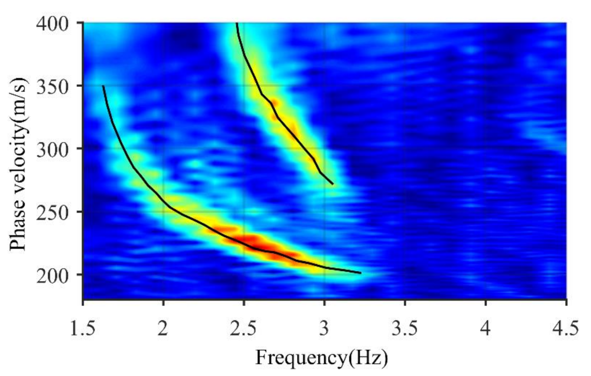
4.2. Analysis of Inversion Result

The initial model parameters are illustrated in

Table 3. Parameters of the initial model.

layer	${\mathit{v}}_{\mathit{p}} \left(\mathbf{m}/\mathbf{s}\right)$	${\mathit{v}}_{\mathit{s}} \left(\mathbf{m}/\mathbf{s}\right)$	$\mathbf{Density}\left(\mathbf{g}/{\mathbf{cm}}^3\right)$	Thickness (m)
1	1500	-	1.0	20
2	1537	238	1.49	50
3	1602	266	1.54	50
4	1667	294	1.60	50
5	1732	322	1.65	50
6	1797	350	1.69	50
7	1863	378	1.74	50
8	1928	405	1.78	50
9	1993	433	1.83	50
10	2057	461	1.87	50
11	2123	489	1.91	50
12	2189	517	1.95	50
13	2254	545	1.99	Inf

. The dispersion of the Scholte wave is mainly affected by the bottom shear wave velocity structure, but is relatively less sensitive to the other parameters. The initial P-wave velocity structure and density structure are determined by the empirical function [36]:

$$v_p=1.511+1.304d-0.714d^2+0.257d^3,$$

(25)

$$v_p=2.3304-0.257\rho +0.4877{\rho }^2,$$

(26)

where $v_p$ is P-wave velocity, $d$ is depth and $\rho$ is density. The initial shear-wave velocity profile is determined from dispersion data, and its semi-infinite layer parameters (maximum) and seabed surface parameters (minimum) are determined from the range of phase velocities based on the empirical relationship [37]:

$$v_s=c_R/0.88,$$

(27)

where $c_R$ is the phase velocity of surface wave. The shear-wave velocity of other layers is linearly distributed by depth. In our inversion, the number of layers in the shear wave velocity profile is determined by minimizing the Bayesian information criterion (BIC) [5]. Here, a model of 13 layers was chosen, with each layer having a constant thickness of 50 m.

The final inversion results are illustrated in Figure 11a, which estimate the shear wave velocity profile along the estimated standard deviation and express the standard deviation as an error bar. A total of 23 unknown parameters were estimated, including 12 shear wave velocities and 11-layer thickness. The sea bottom depth alters from 20 to 700 m, and the shear wave sound velocity ranges from 181–653 m/s. From shallow to deep, the standard deviation is about 50 to 150 m/s. The upper sediments at the bottom of the ocean are extremely soft and have very small shear wave velocities. In addition, low S-wave velocity layers appear at the depth of 200 and 500 m. The actual sedimentary structure under the seabed can be divided into argillaceous layer (clayey silt, silt) and sandy layer. The two kinds of sediments alternate, resulting in frequent alternation of high-speed and low-speed layers. The same conclusion is obtained from the seismic profile of CSDP-2 acoustic well logging in the near sea area in reference [32]. It can be seen from the velocity curve given in the literature that although the overall velocity increases with the increase of depth, it shows the characteristics of alternating change under the background of the overall trend. The theoretical dispersion curves are in strong agreement with the experimental values, as illustrated in Figure 11b.

5. Conclusions

Stiffness matrix methods are introduced in this study for the fundamental and higher mode of Scholte wave dispersion curve computations. It is tested in a vertically transverse isotropic elastic layer, and remains stable for high frequencies in the unlimited range. The dispersion curves of the fundamental mode of the Scholte wave and the fundamental mode of the Rayleigh wave are compared without a fluid layer, and the wave velocity is higher for the fundamental mode when there is no liquid surface. By computing the dispersion curves of different ocean environment models, it is found that when there is a low shear-velocity layer, the coupling phenomenon between the fundamental mode and the first higher-order mode occurs. Due to the large incident angle of high-order modes, it is difficult to reach the critical angle in the layered seabed, i.e., the incident depth is larger. The higher mode dispersion curve appears to be more sensitive to the layered model parameters as compared to the fundamental mode.

In our multi-channel seismic exploration experiment, the Scholte wave generated by the near-sea air gun array is acquired. The fundamental and first-higher mode Scholte wave dispersion curves are extracted from the experimental data, and ocean bottom shear wave profiles are obtained by phase velocity inversion. The thickness and parameters of the topmost layer are estimated with relatively negligible errors. The maximum depth of penetration is nearly 700 m below the sea floor, and the sensitivity is highest at the top layers. The very low shear wave velocities near the sea floor explain the weak excitation of Scholte waves at relatively low frequencies. The inversion results show that the sedimentary structure in the experimental sea area can be divided into a muddy layer and sandy layer, and the two kinds of sediments appear to alternate. As a result, this shear wave velocity structure will be capable of providing significant information regarding the study of seismic processing, offshore field response analysis, and underwater acoustic transmission loss computation in this particular area.

References

1. Kaufmann, R.D.; Xia, J.; Benson, R.C.; Yuhr, L.B.; Casto, D.W.; Park, C.B. Evaluation of MASW data acquired with a hydrophone streamer in a shallow marine environment. J. Environ. Eng. Geophys. 2005, 10, 87–98. [Google Scholar] [CrossRef]
2. Kugler, S.; Bohlen, T.; Bussat, S.; Klein, G. Variability of scholte-wave dispersion in shallow-water marine sediments. J. Environ. Eng. Geophys. 2005, 10, 203–218. [Google Scholar] [CrossRef]
3. Park, C.B.; Miller, R.D.; Xia, J.; Ivanov, J.; Sonnichsen, G.V.; Hunter, J.A.; Good, R.L.; Burns, R.A.; Christian, H. Underwater MASW to evaluate stiffness of water-bottom sediments. Lead. Edge 2005, 24, 724–728. [Google Scholar] [CrossRef]
4. Xuan, N.N.; Dahm, T.; Grevemeyer, I. Inversion of Scholte wave dispersion and waveform modeling for shallow structure of the Ninetyeast Ridge. J. Seismol. 2009, 13, 543–559. [Google Scholar] [CrossRef] [Green Version]
5. Li, C.; Dosso, S.E.; Dong, H.; Yu, D.; Liu, L. Bayesian inversion of multimode interface-wave dispersion from ambient noise. IEEE J. Ocean. Eng. 2012, 37, 407–416. [Google Scholar]
6. Du, S.; Cao, J.; Zhou, S.; Qi, Y.; Jiang, L.; Zhang, Y.; Qiao, C. Observation and inversion of very-low-frequency seismo-acoustic fields in the South China Sea. J. Acoust. Soc. Am. 2020, 148, 3992. [Google Scholar] [CrossRef] [PubMed]
7. Thomson, W.T. Transmission of elastic waves through a stratified solid medium. J. Appl. Phys. 1950, 21, 89–93. [Google Scholar] [CrossRef]
8. Haskell, N.A. The dispersion of surface waves on multilayered media. Bull. Seismol. Soc. Am. 1953, 43, 17–34. [Google Scholar] [CrossRef]
9. Buchen, P.W.; Ben-Hador, R. Free-mode surface-wave computations. Geophys. J. Int. 1996, 124, 869–887. [Google Scholar] [CrossRef]
10. Dunkin, J.W. Computation of modal solutions in layered, elastic media at high frequencies. Bull. Seismol. Soc. Am. 1965, 55, 335–358. [Google Scholar] [CrossRef]
11. Watson, T.H. A note on fast computation of Rayleigh wave dispersion in the multilayered half-space. Bull. Seismol. Soc. Am. 1970, 60, 161–166. [Google Scholar]
12. Kennett, B. Reflections, rays and reverberations. Bull. Seismol. Soc. Am. 1974, 64, 1685–1696. [Google Scholar]
13. Chen, X. A systematic and efficient method of computing normal modes for multilayered half-space. Geophys. J. Int. 2010, 115, 391–409. [Google Scholar] [CrossRef] [Green Version]
14. Hu, S.; Zhao, Y.; Wu, J.; Ge, S. Forward modeling of multichannel Rayleigh wave dispersion curve in laterally inhomogeneous media. Chin. J. Geophys. 2021, 64, 1699–1709. [Google Scholar]
15. Han, C.; Liu, Z.P.; Zhang, R.H.; Zhang, H.L.; Yang, L.I.; Huang, Y.Y.; University, S.J. Numerical simulation of the Rayleigh surface wave two-dimensional physical models. Prog. Geophys. 2017, 32, 357–362. [Google Scholar]
16. Yang, Z.; Chen, X.; Pan, L.; Wang, J.; Xu, J.; Zhang, D. Multi-channel analysis of Rayleigh waves based on Vector Wavenumber Tansformation Method (VWTM). In Geophysical Research Abstracts; EBSCO Industries, Inc.: Birmingham, AL, USA, 2019. [Google Scholar]
17. Kausel, E.; Roësset, J.M. Stiffness matrices for layered soils. Bull. Seismol. Soc. Am. 1981, 71, 1743–1761. [Google Scholar] [CrossRef]
18. Wang, Y.; Rajapakse, R. An exact stiffness method for elastodynamics of a layered orthotropic half-plane. J. Appl. Mech. 1994, 61, 339–348. [Google Scholar] [CrossRef]
19. Rokhlin, S.I.; Wang, L. Stable recursive algorithm for elastic wave propagation in layered anisotropic media: Stiffness matrix method. J. Acoust. Soc. Am. 2002, 112, 822–834. [Google Scholar] [CrossRef] [PubMed]
20. Tan, E.L. Stiffness matrix method with improved efficiency for elastic wave propagation in layered anisotropic media. J. Acoust. Soc. Am. 2005, 118, 3400–3403. [Google Scholar] [CrossRef]
21. El Allouche, N.; van der Neut, J.; Drijkoningen, G. Separation of PS-wave reflections from ultra-shallow water OBC data using elastic wavefield decomposition. In Proceedings of the 75th EAGE Conference & Exhibition incorporating SPE EUROPEC 2013, London, UK, 10–14 June 2013; p. cp-348-00797. [Google Scholar]
22. Richardson, M.D.; Briggs, K.B.; Bentley, S.J.; Walter, D.J.; Orsi, T.H. The effects of biological and hydrodynamic processes on physical and acoustic properties of sediments off the Eel River, California. Mar. Geol. 2002, 182, 121–139. [Google Scholar] [CrossRef]
23. Isse, T.; Kawakatsu, H.; Yoshizawa, K.; Takeo, A.; Shiobara, H.; Sugioka, H.; Ito, A.; Suetsugu, D.; Reymond, D.J.E.; Letters, P.S. Surface wave tomography for the Pacific Ocean incorporating seafloor seismic observations and plate thermal evolution. Earth Planet. Sci. Lett. 2019, 510, 116–130. [Google Scholar] [CrossRef]
24. Zheng, G.; Zhu, H.; Wang, X.; Khan, S.; Li, N.; Xue, Y. Bayesian inversion for geoacoustic parameters in shallow Sea. Sensors 2020, 20, 2150. [Google Scholar] [CrossRef] [PubMed]
25. Bonnel, J.; Dosso, S.E.; Eleftherakis, D.; Chapman, N.R. Trans-dimensional inversion of modal dispersion data on the new england mud patch. IEEE J. Ocean. Eng. 2020, 45, 116–130. [Google Scholar] [CrossRef] [Green Version]
26. Lin, S. Advancements in Active Surface Wave Methods: Modeling, Testing, and Inversion; Iowa State University: Ames, IA, USA, 2014. [Google Scholar]
27. Dosso, S.E.; Dettmer, J. Bayesian matched-field geoacoustic inversion. Inverse Probl. 2011, 27, 055009. [Google Scholar] [CrossRef] [Green Version]
28. Nazarian, S.; Stokoe, K.H., II. In Situ Deyermination of Elastic Moduli of Pavement Syatems by Spectral-Analysis-of-Surface-Waves Method: Practical Aspcts. 1985. Available online: https://trid.trb.org/view/268865 (accessed on 29 July 2021).
29. Lowe, M. Matrix techniques for modeling ultrasonic waves in multilayered media. IEEE Trans. Ultrason. Ferroelectr. Freq. Control 1995, 42, 525–542. [Google Scholar] [CrossRef]
30. Supranata, Y.E. Improving the Uniqueness of Shear Wave Velocity Profiles Derived from the Inversion of Multiple-Mode Surface Wave Dispersion Data; University of Kentucky: Lexington, Kentucky, 2006; Volume 67. [Google Scholar]
31. Ryden, N.; Park, C.B. Fast simulated annealing inversion of surface waves on pavement using phase-velocity spectra. Geophysics 2006, 71, R49–R58. [Google Scholar] [CrossRef]
32. Pico Vila, R. Waves in Fluids and Solids; IntechOpen: London, UK, 2011. [Google Scholar]
33. Boaga, J.; Cassiani, G.; Strobbia, C.L.; Vignoli, G. Mode misidentification in Rayleigh waves: Ellipticity as a cause and a cure. Geophysics 2013, 78, EN17–EN28. [Google Scholar] [CrossRef]
34. Dong, H.; Hovem, J.M.; Frivik, S.A. Estimation of shear wave velocity in seafloor sediment by seismo-acoustic interface waves: A case study for geotechnical application. In Theoretical And Computational Acoustics 2005: (With CD-ROM); World Scientific: Singapore, 2006; pp. 33–43. [Google Scholar]
35. Lang, S.; Kurkjian, A.; McClellan, J.; Morris, C.; Parks, T. Estimating slowness dispersion from arrays of sonic logging waveforms. Geophysics 1987, 52, 530–544. [Google Scholar] [CrossRef]
36. Hamilton, E.L. Vp/Vs and Poisson’s ratios in marine sediments and rocks. J. Acous. Soc. Am. 1979, 66, 1093–1101. [Google Scholar] [CrossRef]
37. Xia, J.; Miller, R.D.; Park, C.B. Estimation of near-surface shear-wave velocity by inversion of Rayleigh waves. Geophysics 1999, 64, 1390–1395. [Google Scholar] [CrossRef] [Green Version]
Figure 1. The applicable methodology of underwater MASW.
Jmse 09 00840 g001
Figure 2. Layered ocean structure with horizontal interfaces.
Jmse 09 00840 g002
Figure 3. Normalized dispersion function of the Stiffness matrix method of model 1 at the frequencies of 5, 10, and 20 Hz, along with its roots (illustrated by circles).
Jmse 09 00840 g003
Figure 4. Fundamental mode dispersion curve of Model 1 (a) and Model 2 (b). The red solid line is the Scholte wave dispersion curve and the blue circles are the Rayleigh wave dispersion curve of the models removing the water layer.
Jmse 09 00840 g004
Figure 5. Fundamental mode Scholte wave penetration depth in the ocean bottom. (a) The model of large layer thickness; (b) the model of smaller layer thickness. In the figure represents the wavelength of Scholte waves (The subscript 1 represents the high frequency and 2 repre-sents the low frequency), and represents the s-wave velocity of the ith layer.
Jmse 09 00840 g005
Figure 6. The dispersion curves of the first nine modes of (a) Model 1 and (b) Model 2.
Jmse 09 00840 g006
Figure 7. Plane waves with different incident angles propagating in the layered model. In the figure λ represents the wavelength of Scholte waves (The subscript 1 represents the high frequency and 2 represents the low frequency), and v s i represents the s-wave velocity of the ith layer.
Jmse 09 00840 g007
Figure 8. (a) The experimental area with survey line (red line). (b) The topographic perturbations along the survey line.
Jmse 09 00840 g008
Figure 9. Signals recorded by a single shot.
Jmse 09 00840 g009
Figure 10. Scholte wave phase velocity dispersion diagram. The extracted fundamental mode and first higher-order mode dispersion data are represented by black curves.
Jmse 09 00840 g010
Figure 11. (a) Inversion results of shear wave velocity profile with an error bar. (b) Comparison between experimental and theoretical dispersion curves.
Jmse 09 00840 g011