
Deep Learning-Based Residual Control Chart for Binary Response


1
Division of Science and Mathematics, University of Minnesota-Morris, Morris, MN 56267, USA
2
Department of Statistics, Pukyong National University, Busan 48513, Korea
*
Author to whom correspondence should be addressed.
Symmetry 2021, 13(8), 1389; https://doi.org/10.3390/sym13081389
Submission received: 7 June 2021
/
Revised: 20 July 2021
/
Accepted: 29 July 2021
/
Published: 31 July 2021
(This article belongs to the Special Issue New Advances and Applications in Statistical Quality Control)
Abstract
:A residual (r) control chart of asymmetrical and non-normal binary response variable with highly correlated explanatory variables is proposed in this research. To avoid multicollinearity between multiple explanatory variables, we employ and compare a neural network regression model and deep learning regression model using Bayesian variable selection (BVS), principal component analysis (PCA), nonlinear PCA (NLPCA) or whole multiple explanatory variables. The advantage of our r control chart is able to process both non-normal and correlated multivariate explanatory variables by employing a neural network model and deep learning model. We prove that the deep learning r control chart is relatively efficient to monitor the simulated and real binary response asymmetric data compared with r control chart of the generalized linear model (GLM) with probit and logit link functions and neural network r control chart.
1. Introduction
The COVID-19 pandemic started at the end of the year 2019. It has dramatically changed the social life of human activity since people fight against the spread of COVID-19 by covering their faces wearing masks and doing social distancing. Artificial intelligence (AI) platform-based contact-free human activity has been more common in our society since the occurrence of the COVID-19 pandemic. Therefore, deep learning and machine learning methods for artificial intelligence have been exponentially developed by software engineers recently. However, applying the deep learning method to the quality control area has not been deeply considered yet even though AI-based products such as smart glasses with optical head-mounted display have been developed in our society rapidly.
Quality improvement is an endless objective in manufacturing industries. To improve the quality of a product, researchers try to reduce process variations by using the statistical process control (SPC) which has been an essential statistical method to complete this objective and monitor industrial processes among the quality control society. Walter A. Shewhart developed this control chart in 1924 and has been named as Shewhart control chart which is a graphical display of the quality characteristic used for the monitoring of the process. The main creative idea by Shewhart is to consider the variability of a production process in terms of statistical viewpoints and analyze the variation of a process into common and special causes. Many variants of the SPC have been developed since then. Many diverse control charts can be found in [1,2]. Now, we have too many SPCs available so that the choice of the appropriate SPC considering symmetric or asymmetric data has become a prime research question among professionals for quality control in manufacturing industries. Asymmetric, big and highly correlated datasets have been produced in our modern society, and those data have asymmetric and non-normal distributions. Therefore, it is difficult for quality control researchers to handle highly correlated and asymmetric data because the current available quality control charts can not handle asymmetrical data. Therefore, it is common to get inaccurate quality control information from the current available control charts. Numerous multivariate control charts such as the Hotelling distribution [3], mulvariate CUSUM [4] and multivariate EWMA [5] have been proposed to monitor a process mean vector. But these multivariate control charts have a difficulty to handle non-normal and asymmetric data because of the estimation issue of the unknown covariance structure. Neural network-based approach to quality control research has been popularly applied. Recently [6] proposed r control charts for binary asymmetrical response variable with highly correlated multivariate covariates by using a single layer neural network regression model.
In this research, we extend the single hidden layer neural network regression-based r control charts for binary asymmetrical data to a deep learning regression model with multiple hidden layers via Bayesian variable selection (BVS), principal component analysis (PCA) and nonlinear PCA (NLPCA) so that our r control chart can solve a multicollinearity problem among independent variables. Reference [7] also proposed Poisson, negative binomial and COM-Poisson-based principal component regression-based r-control charts for monitoring dispersed count data to avoid the multicollinearity problem.
Our research proves that our deep learning r control chart has better efficiency than the current methods [6] while overcoming the multicollinearity issue of high-dimensional correlated multivariate data. Our deep learning r control chart will be evaluated with simulated data and Cleveland heart disease read data found in the UCI machine learning repository.
2. Statistical Methods
This research presents deep learning regression-based r-control charts for binary asymmetrical data with multicollinearity among independent variables. We also compare deep learning regression-based r-control charts with whole data, which means it does not apply one of BVS, PCA, and NLPCA to the whole data, with deep learning regression-based r-control charts with dimension reduction data by applying one of BVS, PCA, and NLPCA to the whole data. In addition, we compare our proposed control chart with the binary response regression models (GLM with logit and probit, and neural network regression model) proposed by [6].
2.1. Bayesian Variable Selection and Dimension Reduction by Principal Component Analysis
Before we apply the proposed control chart to a multivariate dataset, we employ the Bayesian variable selection and PCA methods to avoid the multicollearity issue of the multivariate dataset. First, we introduce Objective Bayesian variable selection in linear models proposed in [8]. We used GibbsBvs function with gZellner prior in BayesVarSel R package and performed the number of iterations = 10,000 and the number of burninng = 100 in the BayesVarSel R package [9] for applying the Bayesian variable selection method to a simulated data and real data, the Cleveland heart disease data [10].
In this paper, the r control chart for binary response regression model with the important selected variables by the BVS is a new proposed SPC method which monitors the binary response variable. The BVS method will be applied to GLM with probit, GLM with logit, neural network and deep learning regression models with simulated and real data. PCA is a statistical dimensional reduction method converting a multivariate data set of correlated variables into a set of values of linearly uncorrelated variables called principal components which account for the variation of the original data.
References [6,7,11] considered PCA method for SPCwith the multivariate highly correlated data. Reference [12] proposed nonlinear principal component analysis (NLPCA) as a kernel eigenvalue problem. Unlike linear PCA, the nonlinear kernel PCA (NLPCA) method is a statistical method for performing a nonlinear form of principal component analysis. To extract five principal components in high-dimensional feature spaces, using kernel PCA, we used the ‘kernlab’ R package [13] which provides the most popular kernel functions. We used Gaussian Radial Basis kernel function with hyperparameter: sigma = 0.2 which is inverse kernel width for the radial basis kernel function.
The r control chart for the binary response regression model with primary principal components by PCA was introduced in [6]. But, in this paper, the r control chart for binary response regression model with primary principal components by the NLPCA is a new statistical process control which monitors the binary response variable as a function of uncorrelated PCs, overcoming a multicollinearity issue among independent variables. The new method will be applied to GLM with probit, GLM with logit, neural network and deep learning regression models with simulated and real data.
2.2. Generalized Linear Model and Neural Network Model for Binary Response Data
The r control charts for binary response regression models, such as the GLM with logit and probit, and neural network regression model were proposed by [6]. The GLM has the following probability density distribution which comes from the exponential family:
where we denote the response variable to be y, the location parameter to be , the dispersion parameter to be , and arbitrary functions to be , , and . In particular, is commonly of the form or with a known weight w, is a cumulant function of , and is a function of y and : for various forms of the three functions, we recommend to see Section 2.2.2 in [14].
We denote to be the linear predictor for the response, , so that is a linear combination of unknown parameters and input variables . A link function g, such that , provides the relationship between the linear predictor and the mean of the distribution function. The link function specifies how to convert the expected value to the linear predictor : i.e.,
As an example, when the response variable follows a Bernoulli distribution with a success probability p, we have . If in (1) we take a logit link function with where , a logit model (or logistic model) is given by
where is the column vector of the fixed-effects regression coefficients. For the (2), it can be written as
The response probability distribution of the GLMs belongs to an exponential family of distributions which employ methods analogous to normal linear methods for the normal data [15,16]. Therefore, for asymmetrical (non-normal) distributed data, the GLM with probit link function may not be the best model. That was the motivation that [6] proposed a neural network model based on the r control chart for better predictive accuracy with the non-normal data.
Artificial neural networks (ANNs) are the same as biological neural networks which imitate human brain activity through computer simulations [17,18,19] The ANN uses the concept of weight to select the highest probability of inhibiting all neurons [17,18,19]. The basic formula of an ANN is a single layer feedforward type of connection among neurons. ANNs have input layers and multiple hidden layers. Lastly, the hidden layers are connected to the output layer, which produces the outputs. Reference [20] proposed a pattern recognition for bivariate process mean shifts using feature-based ANN and [21] proposed a control chart pattern recognition using radial basis function (RBF) neural networks. Recently, Reference [22] proposed statistical process control with intelligence based on the deep learning model and reviewed the neural network-based statistical process control. In this paper, we used the ‘nnet’ R packge [23] for feed-forward neural networks with a single hidden layer, and for the deep learning model, we used the ‘deepnet’ R packge [24] with the backpropagation (BP) algorithm for training feed-forward neural networks by using the ‘nn.predict’ command.
Based on the setup of [6], the r-control charts for binary response data use GLM models with logit and probit link functions, and neural network models employ deviance residuals being independent and asymptotically normally distributed with zero mean and unit variance, i.e., for . In this research, we chose a deviance residual for the GLM models with logit and probit link functions and a neural network model because the R packages for the GLM models with logit and probit link functions and the neural network model have a command for producing the deviance residual. It is easy to compare the residuals from both models, which are the GLM-based model, single hidden layer neural network model and multiple hidden layers deep learning model. Reference [25] proposed Shewhart control limits for the deviance residuals as follows:
where k is defined by the false alarm probability, , and is the average run length (ARL) under the process in-control. The ARL is a measure of the performance of control charts for monitoring a process.
2.3. New Binary Response Statistical Process Control Procedure
Our r control chart for binary response uses the following statistical process control procedures for the deviance residuals:
- Apply the BVS, PCS and NLPCS to input variables and obtain the important selected variables or principal components.
- Fit the binary response regression model by using the binary response variable y and the important selected variables or the principal components through probit link function, logit link function, and neural network or deep learning regression models, respectively.
- Obtain the deviance residuals from each model.
3. Illustrated Examples
With the proposed method in Section 2, we perform the efficiency comparison among the proposed methods with simulated data and real data.
3.1. Simulation Study
With high correlated and non-normal simulated data, we want to compare the r control charts for binary response regression models introduced in the Section 2. So we need to generate high correlated and non-normal simulated data denoting as input variables.
Because of relaxing the assumptions of normality, linearity and independence, copulas have been popular in the research areas of biostatics, econometrics, finance and statistics over the last three decades. A copula is a statistical method to find the dependence structure of multivariate data. By using the copula, we can have the marginal behavior of a random variable and the joint dependence of two random variables. Every joint distribution can be expressed by as where and are marginal distributions.
A bivariate copula is a function , whose domain is the entire unit square with the following three properties:
- (i)
- ;
- (ii)
- ;
- (iii)
- , such that and where and , .
See [26,27] for the definitions of the copula in detail. To construct a highly correlated dependence structure of input variables, we employed two Archimedean copula functions. One is the Clayton copula with a dependence parameter equalling to 3 and the number of dimensions equal to 30, and the other is the Gumbel copula with a dependence parameter equal to 30 and the number of dimensions equalling to 30.
The reason of choosing the Clayton and the Gumbel copulas for generating simulated data in this research is that the Clayton copula is an asymmetric Archimedean copula, exhibiting greater dependence in the negative tail than in the positive and the Gumbel copula is an asymmetric Archimedean copula, exhibiting greater dependence in the positive tail than in the negative.
We generate a random sample of 1000 observations from each copula. The random sample is assigned to as input variables. With each simulated random sample data , we define the coefficients of parameters (’s) to be , , , , , , , , , , , , , , , , , , , , , , , , , , , , , , so that which passes through an inverse logit function. Then, we generate the response variable y randomly by using the Bernoulli distribution with the probability with sample size 1000.
For the one (‘1’) inflated case of binary response data, we added 0.1 to the probability , such as , and for the zero (‘0’) inflated case of binary response data, we subtracted 0.1 from the probability , such as . Additionally, is used for the in-control dispersion case.
In each setup, we perform 1000 different replications of sample size of 1000. Table 1 shows the simulation results. With the simulated data, 70% of data were assigned to the training data and 30% of data were assigned to the test data.
We apply the BVS, PCS, and NLPCS to input variables and then we fit the binary response regression model by using the binary response variable y and the important selected variables or the principal components or the whole data through the probit link function, logit link function, and neural network or deep learning regression models, respectively. We used the ‘nnet’ R packge [23] for feed-forward neural networks with a single hidden layer with 30 neurons by using ‘predict’ command, and for the deep learning model, we used the ‘deepnet’ R packge [24] with the backpropagation (BP) algorithm for training feed-forward neural networks with double hidden layers and (15, 15) neurons by using the ‘nn.predict’ command.
where Root MSE = root mean squared error, , number of observations, , and predicted value of observations.
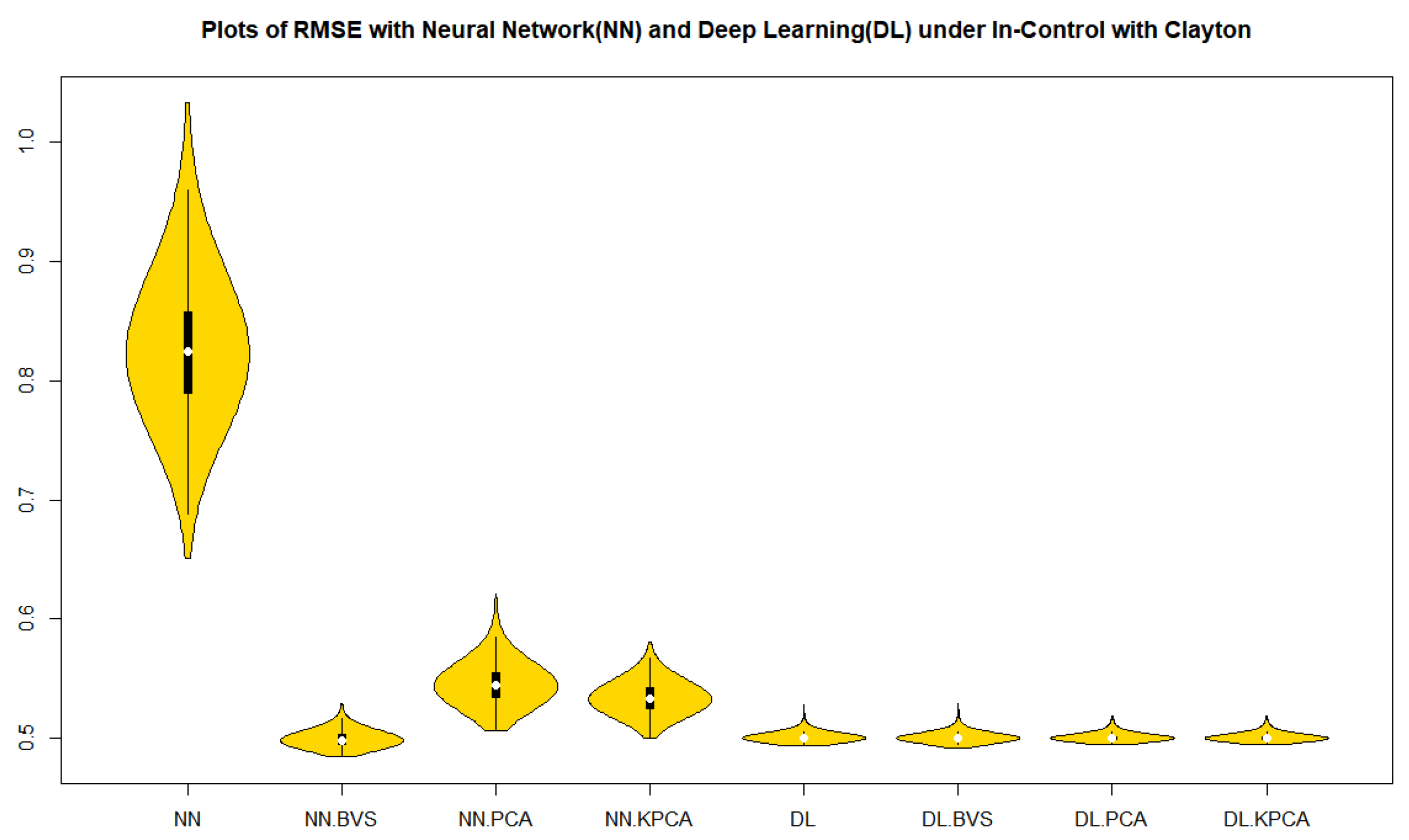
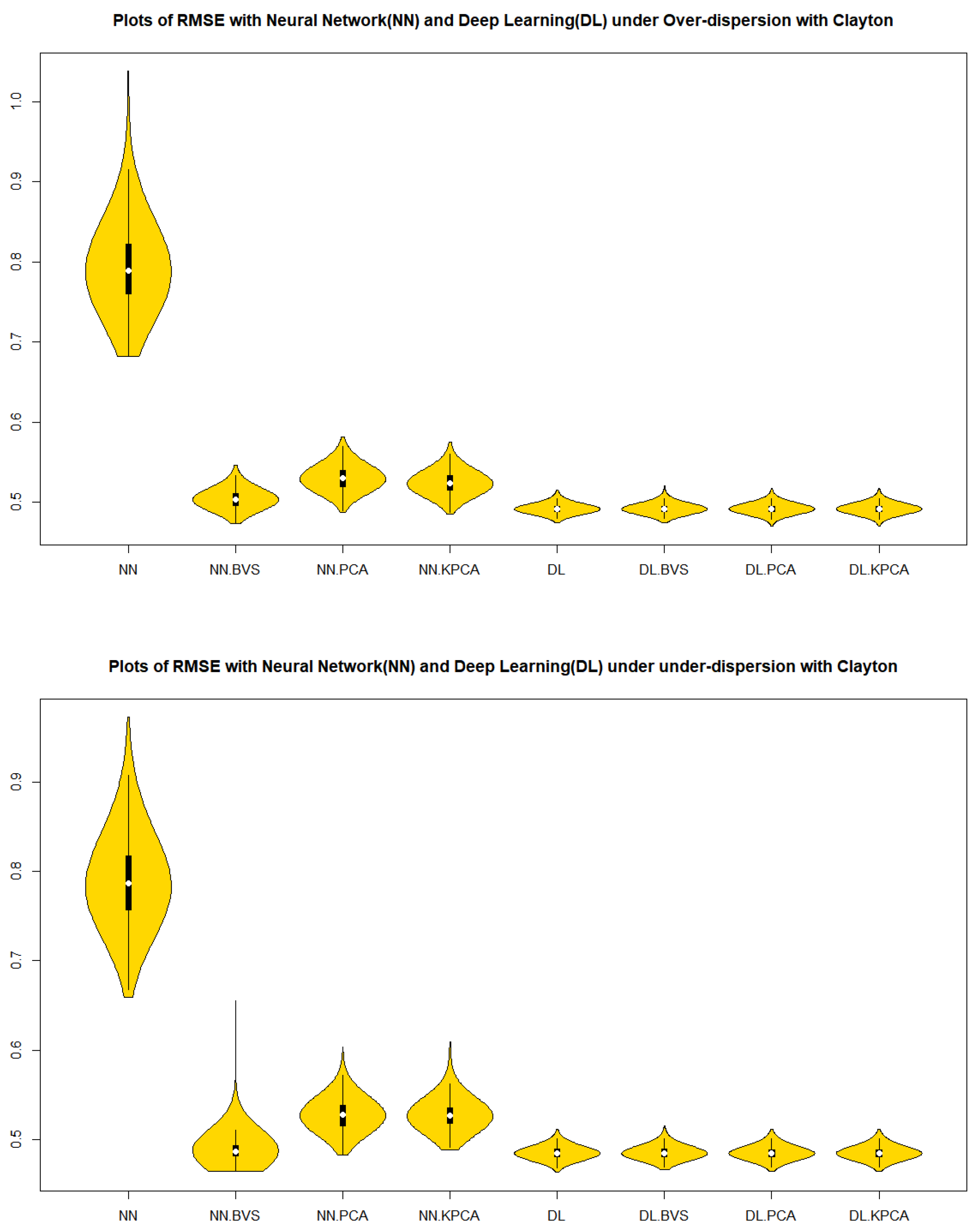
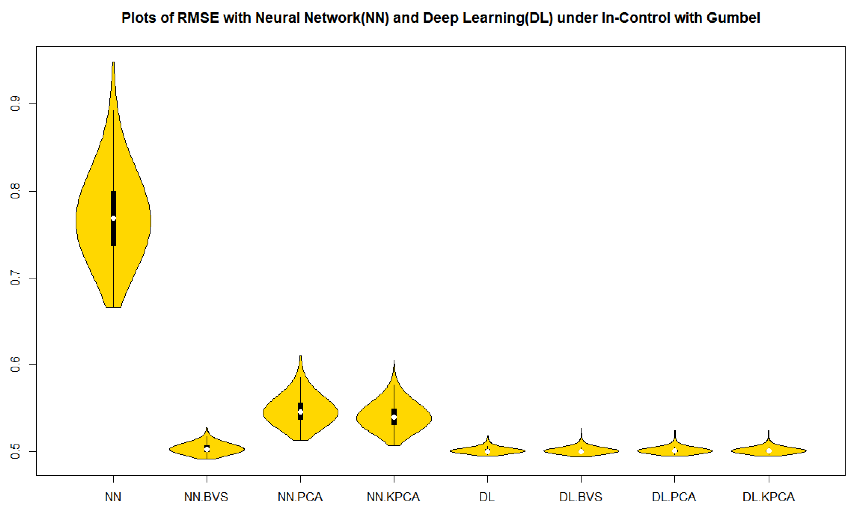
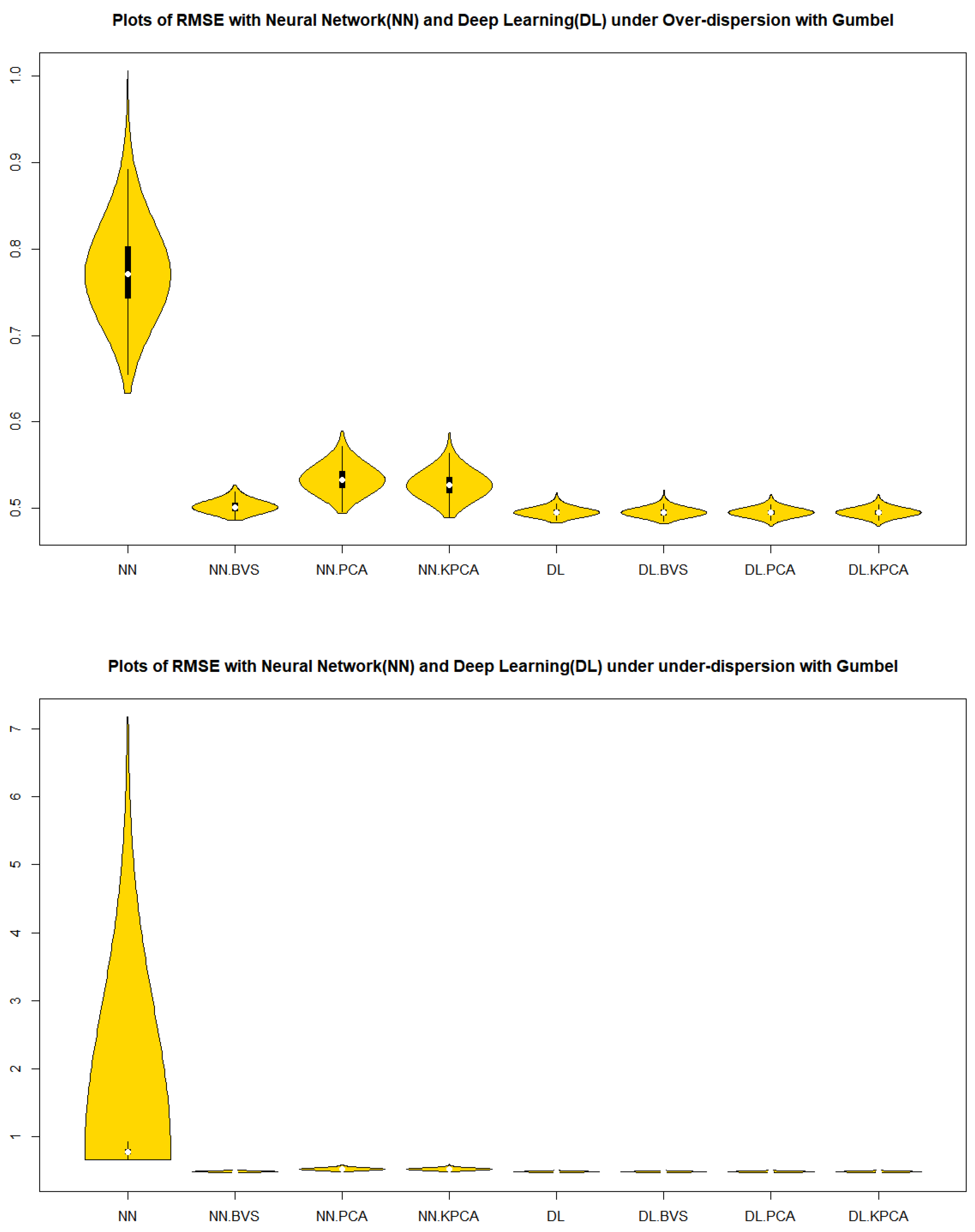
By using the Root MSE Formula (5), we performed the Root MSE of each simulated in-control data of sample size 1000 with 1000 repetitions in Table 1. It is a surprising result that the r-chart based on the deep learning models with BVS, PCS, NLPCS and whole data for both the Clayton and the Gumbel copulas show a superiority to all other cases in Table 1 in terms of the accuracy and precision by mean, median, and interquartile range (IQR).
From Figure 1 and Figure 2 in cases of the in-control, over dispersion and under dispersion, we can observe that the residuals of deep learning regression models with BVS, PCS, NLPCS, and whole data for both the Clayton and Gumbel copulas show a superiority over the neural network regression models with BVS, PCS, NLPCS, and whole data in Table 1 in terms of the precision by a measure of spread, IQR.
With three cases of the in-control, over dispersion, and under dispersion in Table 2, Table 3, Table 4, Table 5, Table 6 and Table 7, we apply the BVS, PCS, and NLPCS to input variables and then we fit the binary response regression model by using the binary response variable y and the important selected variables or the principal components through neural network or deep learning regression models, respectively. By using the deviance residuals for each model and (4) for , we compute the lower control limit (LCL) and upper control limit (UCL) for the process. The expected length of the confidence interval is computed by the average of the length of control limits. The coverage probability is the proportion of the deviance residuals contained in the control limits. The lower control limit and the upper control limit value for the r-chart are calculated by means of y minus and plus its one, two, and three standard deviations.
Mainly, we compare the results for the deep learning regression model and neural network regression model based on BVS, PCA, NLPCA, and whole data because [6] showed that the neural network regression model (Nnet) outperformed the GLMs with probit and logit link functions based on PCA. We found that, for the in-control case, the one-inflated case, and zero-inflated case, the expected lengths of the confidence interval on the deep learning regression model (DL) based on BVS, PCA, NLPCA, and whole data are shorter than in all other cases of Nnet in Table 2, Table 3, Table 4 and Table 5 while, in terms of the coverage probability, the DL is keeping overall higher than the neural network regression model (nnet).
In terms of the ARLs, the coverage probability and the expected length of the confidence interval, we note that the r-chart based on the DL based on whole data for monitoring observations is about the same as the r-chart based on the DL based on BVS, PCA, and NLPCA.
3.2. Real Data Analysis
For the real data application, we used Wisconsin breast cancer data in the R package ‘mlbench’ [23]. The objective of collecting the data was to identify a number of benign or malignant classes. Samples arrive periodically as Dr. Wolberg reports his clinical cases. The database, therefore, reflects this chronological grouping of the data. This grouping information appears immediately below, having been removed from the data itself. Each variable except for the first was converted into 11 primitive numerical attributes with values ranging from 0 through 10. There are 16 missing attribute values. A data frame contained 11 variables ((1) Id (Sample code number), (2) Cl.thickness (Clump Thickness), (3) Cell.size (Uniformity of Cell Size), (4) Cell.shape (Uniformity of Cell Shape), (5) Marg.adhesion (Marginal Adhesion), (6) Epith.c.size (Single Epithelial Cell Size), (7) Bare.nuclei (Bare Nuclei), (8) Bl.cromatin (Bland Chromatin), (9) Normal.nucleoli (Normal Nucleoli), (10) Mitoses, (11) Class), one being a character variable, 9 being ordered or nominal, and 1 target class.
By using the R package ‘missForest’ [28], we imputed the missing data in the Wisconsin breast cancer data. We set the target variable (y) to be Class (“malignant” = 0, “benign” = 1) and 9 input variables except for Id and Class variables in the Wisconsin breast cancer data. We also used the ‘nnet’ R packge [23] with a single hidden layer with 30 neurons by using ‘predict’ command, and for deep learning model, we used the R packge ‘deepnet’ [24] with double hidden layers and (15, 15) neurons by using ‘nn.predict’ command on the Wisconsin breast cancer data. By using the Root MSE formula (5), we performed Root MSE of each random sample data of sample size out of the total number of data (683) with 1000 repetitions in Table 6. It confirms that the r-chart based on the DL models with BVS, PCS, NLPCS and whole data show a superiority to all other cases in Nnet models in Table 6 in terms of the accuracy and precision by mean and interquartile range (IQR).
The expected lengths of the confidence interval on the DL-based on BVS, PCA, NLPCA, and whole real data are shorter than in all other cases of Nnet in Table 7 while, in terms of the coverage probability, DL is overall keeping higher than the Nnet. In terms of the ARLs, the coverage probability and the expected length of the confidence interval, we note that the r-chart based on the DL based on whole real data is about the same as the r-chart based on the DL based on BVS, PCA, and NLPCA.
Therefore, from the simulation study and real data analysis, we confirmed that the DL based r control chart for binary response data on BVS, PCA, NLPCA, and whole real data are superior to the Nnet-based r control chart for binary response data on BVS, PCA, NLPCA, and whole data in terms of the accuracy, precision, coverage probability, and expected length of the confidence interval.
4. Conclusions
In this research, we have presented the binary response DL regression model-based statistical process control r-charts for dispersed binary asymmetrical data with multicollinearity among input variables. We have demonstrated the proposed DL method in terms of the model flexibility and performance by running simulations for various circumstances: in-control, one inflated-, or zero inflated-dispersion data. With both simulated data and real data, our DL proposed methods based on BVS, PCA, NLPCA, and whole data have shown a superiority of performance compared with the binary response regression model-based statistical control r-charts with the GLM with probit and logit link function models and Nnet based on BVS, PCA, NLPCA and whole data. We also showed that the binary response DL regression model-based statistical process control r-charts for dispersed binary asymmetrical data with multicollinearity among input variables does not need dimension reduction methods such as BVS, PCA, and NLPCA because the results with the dimension reduction methods, such as BVS, PCA, and NLPCA are the same as the results without the dimension reduction methods. Our proposed approach by deep learning is superior in handling cases of dispersed binary asymmetrical data with multicollinearity among explanatory variables. The conclusion in this research is that for the high-dimensional correlated multivariate covariate data, the binary control chart by DL is a good statistical process control method. Our proposed binary control chart by DL can be applied to improve the quality control of visual fault detection medical equipment devices such a full-body X-ray scanner or brain functional magnetic resonance imaging scanner or a computed tomography (CT) scanner for detecting cancers. Our future research will be the general version of DL-based SPC for categorical data or continuous data or mixed data for categorical and continuous data. We will also apply our proposed method to a multi-stage SPC for binary outcome variables given the covariates.
Author Contributions
J.M.K. designed the model, analyzed the data and wrote the paper. I.D.H. formulated the conceptual framework, designed the model, obtained inference, and wrote the paper. Both authors cooperated to revise the paper. Both authors have read and agreed to the published version of the manuscript.
Funding
This work was supported by the Basic Science Research Program through the National Research Foundation of Korea (NRF) funded by the Ministry of Education (No. NRF-2020R1F1A1A01056987).
Conflicts of Interest
The authors declare no conflict of interest.
References
- Montgomery, D.C. Statistical Quality Control, 7th ed.; John Wiley and Sons Press: New York, NY, USA, 2012. [Google Scholar]
- Qiu, P. Introduction to Statistical Process Control, 1st ed.; Chapman & Hall/CRC Texts in Statistical Science: Boca Raton, FL, USA, 2013. [Google Scholar]
- Hotelling, H. Multivariate Quality Control; McGraw-Hill: New York, NY, USA, 1947. [Google Scholar]
- Crosier, R.B. Multivariate generalizations of cumulative sum qualitycontrol schemes. Technometrics 1988, 30, 291–303. [Google Scholar] [CrossRef]
- Lowry, C.A.; Woodall, W.H.; Champ, C.W.; Rigdon, S.E. Multivariate exponentially weighted moving average control chart. Technometrics 1992, 34, 46–53. [Google Scholar] [CrossRef]
- Kim, J.-M.; Wang, N.; Liu, Y.; Park, K. Residual Control Chart for Binary Response with Multicollinearity Covariates by Neural Network Model. Symmetry 2020, 12, 381. [Google Scholar] [CrossRef] [Green Version]
- Park, K.; Kim, J.-M.; Jung, D. GLM-based statistical control r-charts for dispersed count data with multicollinearity between input variables. Qual. Reliab. Eng. Int. 2018, 34, 1103–1109. [Google Scholar] [CrossRef]
- Garcia-Donato, G.; Forte, A. Bayesian Testing, Variable Selection and Model Averaging in Linear Models using R with BayesVarSel. R J. 2018, 10, 329. [Google Scholar] [CrossRef] [Green Version]
- Forte, A. Bayes Factors, Model Choice and Variable Selection in Linear Models; R Package, BayesVarSel; R Foundation for Statistical Computing: Vienna, Austria, 2020. [Google Scholar]
- Leisch, F.; Dimitriadou, E. Machine Learning Benchmark Problems; R Package, mlbench; R Foundation for Statistical Computing: Vienna, Austria, 2015. [Google Scholar]
- Kim, J.-M.; Liu, Y.; Wang, N. Multi-stage change point detection with copula conditional distribution with PCA and functional PCA. Mathematics 2020, 8, 1777. [Google Scholar] [CrossRef]
- Schölkopf, B.; Smola, A.; Müller, K.-R. Nonlinear Component Analysis as a Kernel Eigenvalue Problem. Neural Comput. 1998, 10, 1299–1319. [Google Scholar] [CrossRef] [Green Version]
- Karatzoglou, A.; Smola, A.; Hornik, K.; National ICT Australia; Maniscalco, M.A.; Teo, C.H. Kernel-Based Machine Learning Lab; R Package, Kernlab; R Foundation for Statistical Computing: Vienna, Austria, 2019. [Google Scholar]
- McCullagh, P.; Nelder, J.A. Generalized Linear Models; Chapman and Hall: New York, NY, USA, 1989. [Google Scholar]
- Myers, R.H.; Montgomery, D.C.; Vining, G.G. Generalized Linear Models, with Applications in Engineering and the Sciences; John Wiley and Sons Press: New York, NY, USA, 2002. [Google Scholar]
- Nelder, J.A.; Wendderburn, R.W.M. Generalized linear model. J. R. Stat. Hencec. A 1972, 35, 370–384. [Google Scholar] [CrossRef]
- Agatonovic-Kustrin, S.; Beresford, R. Basic concepts of artificial neural network (ANN) modeling and its application in pharmaceutical research. J. Pharm. Biomed. Anal. 2000, 22, 717–727. [Google Scholar] [CrossRef]
- LeCun, Y.; Bengio, Y.; Hinton, G. Deep learning. Nature 2015, 521, 436. [Google Scholar] [CrossRef] [PubMed]
- Hassabis, D.; Kumaran, D.; Summerfield, C.; Botvinick, M. Neuroscience-inspired artificial intelligence. Neuron 2017, 95, 245–258. [Google Scholar] [CrossRef] [PubMed] [Green Version]
- Masood, I.; Hassan, A. Pattern Recognition for Bivariate Process Mean Shifts Using Feature-Based Artificial Neural Network. Int. J. Adv. Manuf. Technol. 2013, 66, 1201–1218. [Google Scholar] [CrossRef] [Green Version]
- Addeh, A.; Khormali, A.; Golilarz, N.A. Control Chart Pattern Recognition Using RBF Neural Network with New Training Algorithm and Practical Features. ISA Trans. 2018, 79, 202–216. [Google Scholar] [CrossRef] [PubMed]
- Zan, T.; Liu, Z.; Su, Z.; Wang, M.; Gao, X.; Chen, D. Statistical Process Control with Intelligence Based on the Deep Learning Model. Appl. Sci. 2020, 10, 308. [Google Scholar] [CrossRef] [Green Version]
- Ripley, B.; Venables, W. Feed-Forward Neural Networks and Multinomial Log-Linear Models; R Package, mlbench; R Foundation for Statistical Computing: Vienna, Austria, 2016. [Google Scholar]
- Rong, X. Deep Learning Toolkit in R; R Package, Deepnet; R Foundation for Statistical Computing: Vienna, Austria, 2015. [Google Scholar]
- Skinner, K.R.; Montgomery, D.C.; Runger, G.C. Process monitoring for multiple count data using generalized linear model-based control charts. Int. J. Prod. Res. 2003, 41, 1167–1180. [Google Scholar] [CrossRef]
- Nelsen, R.B. An Introduction to Copulas, 2th ed.; Springer: New York, NY, USA, 2006. [Google Scholar]
- Kim, J.-M. A Review of Copula Methods for Measuring Uncertainty in Finance and Economics. Quant. Bio-Sci. 2020, 39, 81–90. [Google Scholar]
- Stekhoven, D.J. Nonparametric Missing Value Imputation Using Random Forest; R Package, missForest; R Foundation for Statistical Computing: Vienna, Austria, 2016. [Google Scholar]
Figure 1.
Violin plots of RMSE with Clayton Copula simulated data.


Figure 2.
Violin plots of RMSE with Gumbel Copula simulated data.


Table 1.
Root MSE of simulated in-control data with 1000 Repetitions.
| Clayton Copula | Model | Q1 | MEDIAN | MEAN | Q3 | IQR |
| Whole Data | Nnet | 0.7898 | 0.824 | 0.827 | 0.858 | 0.068 |
| BVS | Nnet | 0.4949 | 0.499 | 0.5 | 0.504 | 0.009 |
| PCA | Nnet | 0.5348 | 0.544 | 0.546 | 0.555 | 0.02 |
| NLPCA | Nnet | 0.5255 | 0.533 | 0.534 | 0.542 | 0.017 |
| Whole Data | DL | 0.4993 | 0.5 | 0.501 | 0.502 | 0.003 |
| BVS | DL | 0.4991 | 0.5 | 0.501 | 0.502 | 0.003 |
| PCA | DL | 0.4993 | 0.5 | 0.501 | 0.502 | 0.003 |
| NLPCA | DL | 0.4993 | 0.5 | 0.501 | 0.502 | 0.003 |
| PCA | Logit | 0.7288 | 0.766 | 0.767 | 0.803 | 0.074 |
| PCA | Probit | 0.7045 | 0.731 | 0.732 | 0.757 | 0.053 |
| NLPCA | Logit | 0.7207 | 0.754 | 0.755 | 0.791 | 0.071 |
| NLPCA | Probit | 0.7042 | 0.729 | 0.73 | 0.757 | 0.053 |
| Gumbel Copula | Model | Q1 | MEDIAN | MEAN | Q3 | IQR |
| Whole Data | Nnet | 0.7372 | 0.769 | 0.771 | 0.799 | 0.062 |
| BVS | Nnet | 0.4996 | 0.503 | 0.503 | 0.507 | 0.007 |
| PCA | Nnet | 0.537 | 0.546 | 0.547 | 0.556 | 0.019 |
| NLPCA | Nnet | 0.5309 | 0.539 | 0.541 | 0.549 | 0.018 |
| Whole Data | DL | 0.4998 | 0.5 | 0.501 | 0.502 | 0.002 |
| BVS | DL | 0.4998 | 0.5 | 0.501 | 0.502 | 0.002 |
| PCA | DL | 0.4998 | 0.501 | 0.501 | 0.502 | 0.002 |
| NLPCA | DL | 0.4998 | 0.501 | 0.501 | 0.502 | 0.002 |
| PCA | Logit | 0.6643 | 0.691 | 0.694 | 0.723 | 0.059 |
| PCA | Probit | 0.6751 | 0.697 | 0.698 | 0.721 | 0.046 |
| NLPCA | Logit | 0.6656 | 0.693 | 0.696 | 0.728 | 0.062 |
| NLPCA | Probit | 0.6748 | 0.697 | 0.698 | 0.721 | 0.046 |
Table 2.
ARLs of simulated data by Clayton Copula.
| Clayton Copula | Whole Data | Nnet | DL | ||||
| In-Control | ARL | 3.334 | 20.71 | 112.746 | 2.02 | NA | NA |
| CL | 0 | 0 | 0 | 0.002 | 0.002 | 0.002 | |
| LCL | −0.821 | −1.642 | −2.464 | −0.498 | −0.998 | −1.498 | |
| UCL | 0.822 | 1.643 | 2.464 | 0.501 | 1.001 | 1.501 | |
| CI Length | 1.643 | 3.285 | 4.928 | 1 | 1.999 | 2.999 | |
| Coverage | 0.7 | 0.955 | 0.994 | 0.55 | 1 | 1 | |
| Over-dispersion | ARL | 3.292 | 22.289 | 106.563 | 2.695 | NA | NA |
| CL | 0.002 | 0.002 | 0.002 | −0.002 | −0.002 | −0.002 | |
| LCL | −0.81 | −1.621 | −2.432 | −0.495 | −0.988 | −1.481 | |
| UCL | 0.813 | 1.624 | 2.435 | 0.491 | 0.983 | 1.476 | |
| CI Length | 1.622 | 3.245 | 4.867 | 0.986 | 1.971 | 2.957 | |
| Coverage | 0.699 | 0.956 | 0.994 | 0.585 | 1 | 1 | |
| Under-dispersion | ARL | 3.261 | 22.502 | 112.493 | 2.561 | NA | NA |
| CL | −0.001 | −0.002 | −0.001 | 0.001 | 0.001 | 0.002 | |
| LCL | −0.801 | −1.601 | −2.4 | −0.485 | −0.971 | −1.457 | |
| UCL | 0.799 | 1.598 | 2.398 | 0.487 | 0.974 | 1.46 | |
| CI Length | 1.6 | 3.199 | 4.798 | 0.972 | 1.945 | 2.917 | |
| Coverage | 0.699 | 0.956 | 0.995 | 0.617 | 1 | 1 | |
| Clayton Copula | BVS | Nnet | DL | ||||
| In-Control | ARL | 2.264 | 138.234 | 130.333 | 2.111 | NA | NA |
| CL | 0.001 | 0.001 | 0.001 | 0.001 | 0.001 | 0.001 | |
| LCL | −0.504 | −1.009 | −1.513 | −0.498 | −0.998 | −1.498 | |
| UCL | 0.506 | 1.01 | 1.515 | 0.501 | 1.001 | 1.501 | |
| CI Length | 1.009 | 2.019 | 3.028 | 1 | 1.999 | 2.999 | |
| Coverage | 0.548 | 0.999 | 1 | 0.543 | 1 | 1 | |
| Over-dispersion | ARL | 2.476 | 111.384 | 146.131 | 2.534 | NA | NA |
| CL | 0 | 0 | 0 | 0 | 0 | 0 | |
| LCL | −0.513 | −1.026 | −1.54 | −0.493 | −0.986 | −1.479 | |
| UCL | 0.513 | 1.027 | 1.54 | 0.493 | 0.986 | 1.479 | |
| CI Length | 1.026 | 2.053 | 3.079 | 0.986 | 1.972 | 2.957 | |
| Coverage | 0.587 | 0.995 | 1 | 0.584 | 1 | 1 | |
| Under-dispersion | ARL | 2.486 | 149.789 | 181.353 | 2.623 | NA | NA |
| CL | −0.002 | −0.002 | −0.002 | −0.001 | −0.001 | −0.001 | |
| LCL | −0.494 | −0.986 | −1.478 | −0.488 | −0.974 | −1.46 | |
| UCL | 0.49 | 0.982 | 1.474 | 0.485 | 0.971 | 1.457 | |
| CI Length | 0.984 | 1.968 | 2.952 | 0.973 | 1.945 | 2.917 | |
| Coverage | 0.597 | 0.999 | 1 | 0.616 | 1 | 1 | |
Table 3.
ARLs of Simulated Data by Clayton Copula.
| Clayton Copula | PCA | Nnet | DL | ||||
| In-Control | ARL | 2.585 | 82.355 | 132.437 | 2.135 | NA | NA |
| CL | −0.001 | −0.001 | −0.001 | −0.002 | −0.002 | −0.002 | |
| LCL | −0.545 | −1.088 | −1.632 | −0.502 | −1.002 | −1.501 | |
| UCL | 0.543 | 1.086 | 1.63 | 0.498 | 0.997 | 1.497 | |
| CI Length | 1.087 | 2.175 | 3.262 | 1 | 1.999 | 2.998 | |
| Coverage | 0.61 | 0.99 | 0.999 | 0.549 | 1 | 1 | |
| Over-dispersion | ARL | 2.727 | 73.39 | 147.581 | 2.365 | NA | NA |
| CL | 0.001 | 0.001 | 0.001 | −0.001 | −0.001 | −0.001 | |
| LCL | −0.537 | −1.074 | −1.611 | −0.493 | −0.986 | −1.479 | |
| UCL | 0.538 | 1.076 | 1.613 | 0.492 | 0.985 | 1.477 | |
| CI Length | 1.075 | 2.15 | 3.225 | 0.985 | 1.971 | 2.956 | |
| Coverage | 0.613 | 0.988 | 0.999 | 0.586 | 1 | 1 | |
| Under-dispersion | ARL | 2.597 | 71.143 | 143.474 | 2.593 | NA | NA |
| CL | 0.003 | 0.003 | 0.003 | 0.004 | 0.004 | 0.004 | |
| LCL | −0.528 | −1.06 | −1.591 | −0.483 | −0.97 | −1.457 | |
| UCL | 0.534 | 1.065 | 1.597 | 0.491 | 0.978 | 1.465 | |
| CI Length | 1.063 | 2.125 | 3.188 | 0.974 | 1.948 | 2.922 | |
| Coverage | 0.614 | 0.987 | 0.999 | 0.613 | 1 | 1 | |
| Clayton Copula | NLPCA | Nnet | DL | ||||
| In-Control | ARL | 2.448 | 105.494 | 143.163 | 2.135 | NA | NA |
| CL | −0.001 | −0.001 | −0.001 | −0.002 | −0.002 | −0.002 | |
| LCL | −0.536 | −1.071 | −1.605 | −0.502 | −1.002 | −1.501 | |
| UCL | 0.533 | 1.068 | 1.603 | 0.498 | 0.997 | 1.497 | |
| CI Length | 1.069 | 2.139 | 3.208 | 1 | 1.999 | 2.998 | |
| Coverage | 0.592 | 0.994 | 1 | 0.549 | 1 | 1 | |
| Over-dispersion | ARL | 2.478 | 95.062 | 135.056 | 2.365 | NA | NA |
| CL | 0 | 0 | 0 | −0.001 | −0.001 | −0.001 | |
| LCL | −0.528 | −1.056 | −1.584 | −0.493 | −0.986 | −1.479 | |
| UCL | 0.528 | 1.056 | 1.584 | 0.492 | 0.985 | 1.477 | |
| CI Length | 1.056 | 2.112 | 3.168 | 0.985 | 1.971 | 2.956 | |
| Coverage | 0.596 | 0.992 | 1 | 0.586 | 1 | 1 | |
| Under-dispersion | ARL | 2.574 | 90.481 | 141.241 | 2.593 | NA | NA |
| CL | 0.004 | 0.004 | 0.004 | 0.004 | 0.004 | 0.004 | |
| LCL | −0.517 | −1.038 | −1.559 | −0.483 | −0.97 | −1.457 | |
| UCL | 0.525 | 1.046 | 1.567 | 0.491 | 0.978 | 1.465 | |
| CI Length | 1.042 | 2.084 | 3.126 | 0.974 | 1.948 | 2.922 | |
| Coverage | 0.603 | 0.992 | 1 | 0.613 | 1 | 1 | |
Table 4.
ARLs of simulated data by Gumbel Copula.
| Gumbel Copula | Whole Data | Nnet | DL | ||||
| In-Control | ARL | 3.397 | 21.495 | 108.616 | 2.113 | NA | NA |
| CL | 0.002 | 0.002 | 0.002 | 0.001 | 0.001 | 0.001 | |
| LCL | −0.793 | −1.588 | −2.383 | −0.499 | −0.999 | −1.498 | |
| UCL | 0.797 | 1.592 | 2.386 | 0.501 | 1.001 | 1.500 | |
| CI Length | 1.590 | 3.179 | 4.769 | 1.000 | 1.999 | 2.999 | |
| Coverage | 0.716 | 0.955 | 0.994 | 0.549 | 1.000 | 1.000 | |
| Over-dispersion | ARL | 3.336 | 21.692 | 109.006 | 2.484 | NA | NA |
| CL | 0.004 | 0.004 | 0.004 | −0.001 | −0.001 | −0.001 | |
| LCL | −0.778 | −1.559 | −2.340 | −0.493 | −0.986 | −1.479 | |
| UCL | 0.785 | 1.566 | 2.347 | 0.492 | 0.985 | 1.478 | |
| CI Length | 1.562 | 3.124 | 4.687 | 0.986 | 1.971 | 2.957 | |
| Coverage | 0.712 | 0.954 | 0.994 | 0.585 | 1.000 | 1.000 | |
| Under-dispersion | ARL | 3.684 | 21.393 | 110.314 | 2.582 | NA | NA |
| CL | −0.004 | −0.004 | −0.004 | 0.001 | 0.001 | 0.001 | |
| LCL | −0.772 | −1.540 | −2.308 | −0.486 | −0.973 | −1.459 | |
| UCL | 0.765 | 1.533 | 2.301 | 0.487 | 0.974 | 1.460 | |
| CI Length | 1.536 | 3.073 | 4.609 | 0.973 | 1.946 | 2.919 | |
| Coverage | 0.712 | 0.955 | 0.994 | 0.615 | 1.000 | 1.000 | |
| Gumbel Copula | BVS | Nnet | DL | ||||
| In-Control | ARL | 2.217 | 129.387 | 156.500 | 2.088 | NA | NA |
| CL | 0.002 | 0.002 | 0.002 | 0.001 | 0.001 | 0.001 | |
| LCL | −0.504 | −1.010 | −1.515 | −0.499 | −0.998 | −1.498 | |
| UCL | 0.507 | 1.013 | 1.518 | 0.501 | 1.001 | 1.500 | |
| CI Length | 1.011 | 2.022 | 3.033 | 0.999 | 1.999 | 2.998 | |
| Coverage | 0.547 | 0.999 | 1.000 | 0.543 | 1.000 | 1.000 | |
| Over-dispersion | ARL | 2.350 | 137.165 | 157.292 | 2.316 | NA | NA |
| CL | 0.000 | 0.000 | 0.000 | 0.001 | 0.001 | 0.001 | |
| LCL | −0.499 | −0.998 | −1.497 | −0.492 | −0.985 | −1.478 | |
| UCL | 0.499 | 0.997 | 1.496 | 0.493 | 0.986 | 1.479 | |
| CI Length | 0.998 | 1.995 | 2.993 | 0.986 | 1.971 | 2.957 | |
| Coverage | 0.572 | 0.999 | 1.000 | 0.585 | 1.000 | 1.000 | |
| Under-dispersion | ARL | 2.504 | 129.826 | 119.947 | 2.592 | NA | NA |
| CL | 0.000 | 0.000 | 0.000 | 0.001 | 0.001 | 0.001 | |
| LCL | −0.494 | −0.987 | −1.480 | −0.486 | −0.972 | −1.459 | |
| UCL | 0.493 | 0.986 | 1.479 | 0.487 | 0.974 | 1.460 | |
| CI Length | 0.986 | 1.973 | 2.959 | 0.973 | 1.946 | 2.919 | |
| Coverage | 0.599 | 0.999 | 1.000 | 0.615 | 1.000 | 1.000 | |
Table 5.
ARLs of simulated data by Gumbel Copula.
| Gumbel Copula | PCA | Nnet | DL | ||||
| In-Control | ARL | 2.640 | 87.182 | 153.242 | 2.153 | NA | NA |
| CL | 0.001 | 0.001 | 0.001 | 0.001 | 0.001 | 0.001 | |
| LCL | −0.540 | −1.081 | −1.622 | −0.499 | −0.998 | −1.498 | |
| UCL | 0.543 | 1.084 | 1.625 | 0.501 | 1.001 | 1.500 | |
| CI Length | 1.082 | 2.165 | 3.247 | 1.000 | 1.999 | 2.999 | |
| Coverage | 0.607 | 0.990 | 0.999 | 0.546 | 1.000 | 1.000 | |
| Over-dispersion | ARL | 2.522 | 83.406 | 146.587 | 2.231 | NA | NA |
| CL | −0.001 | −0.001 | −0.001 | −0.001 | −0.001 | −0.001 | |
| LCL | −0.536 | −1.070 | −1.605 | −0.493 | −0.986 | −1.479 | |
| UCL | 0.534 | 1.068 | 1.603 | 0.492 | 0.985 | 1.478 | |
| CI Length | 1.069 | 2.139 | 3.208 | 0.986 | 1.971 | 2.957 | |
| Coverage | 0.607 | 0.989 | 0.999 | 0.585 | 1.000 | 1.000 | |
| Under-dispersion | ARL | 2.428 | 76.504 | 142.214 | 2.440 | NA | NA |
| CL | −0.002 | −0.002 | −0.002 | −0.001 | −0.001 | −0.001 | |
| LCL | −0.527 | −1.053 | −1.578 | −0.487 | −0.973 | −1.460 | |
| UCL | 0.524 | 1.050 | 1.575 | 0.485 | 0.971 | 1.458 | |
| CI Length | 1.051 | 2.103 | 3.154 | 0.972 | 1.945 | 2.917 | |
| Coverage | 0.612 | 0.988 | 0.999 | 0.616 | 1.000 | 1.000 | |
| Gumbel Copula | NLPCA | Nnet | DL | ||||
| In-Control | ARL | 2.519 | 104.428 | 145.605 | 2.153 | NA | NA |
| CL | 0.002 | 0.002 | 0.002 | 0.001 | 0.001 | 0.001 | |
| LCL | −0.534 | −1.069 | −1.605 | −0.499 | −0.998 | −1.498 | |
| UCL | 0.537 | 1.072 | 1.608 | 0.501 | 1.001 | 1.500 | |
| CI Length | 1.071 | 2.142 | 3.213 | 1.000 | 1.999 | 2.999 | |
| Coverage | 0.595 | 0.994 | 1.000 | 0.546 | 1.000 | 1.000 | |
| Over-dispersion | ARL | 2.371 | 96.315 | 151.893 | 2.231 | NA | NA |
| CL | −0.001 | −0.001 | −0.001 | −0.001 | −0.001 | −0.001 | |
| LCL | −0.530 | −1.058 | −1.587 | −0.493 | −0.986 | −1.479 | |
| UCL | 0.528 | 1.057 | 1.586 | 0.492 | 0.985 | 1.478 | |
| CI Length | 1.058 | 2.115 | 3.173 | 0.986 | 1.971 | 2.957 | |
| Coverage | 0.598 | 0.992 | 1.000 | 0.585 | 1.000 | 1.000 | |
| Under-dispersion | ARL | 2.480 | 93.172 | 135.882 | 2.440 | NA | NA |
| CL | −0.002 | −0.002 | −0.002 | −0.001 | −0.001 | −0.001 | |
| LCL | −0.523 | −1.045 | −1.566 | −0.487 | −0.973 | −1.460 | |
| UCL | 0.519 | 1.041 | 1.562 | 0.485 | 0.971 | 1.458 | |
| CI Length | 1.043 | 2.085 | 3.128 | 0.972 | 1.945 | 2.917 | |
| Coverage | 0.606 | 0.991 | 1.000 | 0.616 | 1.000 | 1.000 | |
Table 6.
RMSE with Cleveland heart disease data.
| Q1 | MEDIAN | MEAN | Q3 | IQR | ||
|---|---|---|---|---|---|---|
| Whole Data | Nnet | 0.3908 | 0.421 | 0.637 | 0.461 | 0.071 |
| BVS | Nnet | 0.3727 | 0.408 | 2.372 | 0.498 | 0.125 |
| PCA | Nnet | 0.6272 | 0.671 | 0.673 | 0.716 | 0.089 |
| NLPCA | Nnet | 0.499 | 0.527 | 1.223 | 1.339 | 0.84 |
| Whole Data | DL | 0.4977 | 0.5 | 0.5018 | 0.5041 | 0.0064 |
| BVS | DL | 0.4977 | 0.4999 | 0.5018 | 0.5039 | 0.0062 |
| PCA | DL | 0.4976 | 0.5 | 0.5016 | 0.5039 | 0.0063 |
| NLPCA | DL | 0.4979 | 0.5003 | 0.502 | 0.5042 | 0.0063 |
Table 7.
ARLs, CIs, and coverage with Cleveland heart disease Data.
| Nnet | DL | |||||
| Whole Data | ||||||
| ARL | 8.644 | 17.071 | 43.735 | 2.220 | NA | NA |
| CL | −0.119 | −0.119 | −0.119 | 0.006 | 0.006 | 0.006 |
| LCL | −2.481 | −4.842 | −7.204 | −0.494 | −0.993 | −1.492 |
| UCL | 2.243 | 4.604 | 6.966 | 0.505 | 1.004 | 1.503 |
| CI Length | 4.723 | 9.446 | 14.169 | 0.998 | 1.997 | 2.995 |
| Coverage | 0.769 | 0.918 | 0.996 | 0.549 | 1.000 | 1.000 |
| Nnet | DL | |||||
| BVS | ||||||
| ARL | 10.099 | 22.687 | 21.988 | 2.165 | NA | NA |
| CL | 0.105 | 0.105 | 0.105 | 0.002 | 0.002 | 0.002 |
| LCL | −1.111 | −2.326 | −3.542 | −0.497 | −0.996 | −1.495 |
| UCL | 1.321 | 2.537 | 3.753 | 0.501 | 1.001 | 1.500 |
| CI Length | 2.432 | 4.863 | 7.295 | 0.998 | 1.996 | 2.995 |
| Coverage | 0.756 | 0.987 | 0.990 | 0.550 | 1.000 | 1.000 |
| Nnet | DL | |||||
| PCA | ||||||
| ARL | 7.253 | 16.202 | 53.460 | 2.157 | NA | NA |
| CL | −0.012 | −0.012 | −0.012 | 0.005 | 0.005 | 0.005 |
| LCL | −0.646 | −1.281 | −1.915 | −0.494 | −0.993 | −1.493 |
| UCL | 0.623 | 1.257 | 1.891 | 0.504 | 1.003 | 1.502 |
| CI Length | 1.269 | 2.538 | 3.807 | 0.998 | 1.996 | 2.995 |
| Coverage | 0.765 | 0.906 | 0.998 | 0.549 | 1.000 | 1.000 |
| NLPCA | ||||||
| ARL | 3.227 | 19.832 | 44.864 | 2.179 | NA | NA |
| CL | −0.003 | −0.003 | −0.003 | 0.003 | 0.003 | 0.003 |
| LCL | −0.676 | −1.348 | −2.020 | −0.496 | −0.995 | −1.494 |
| UCL | 0.669 | 1.341 | 2.013 | 0.501 | 1.000 | 1.499 |
| CI Length | 1.345 | 2.689 | 4.034 | 0.998 | 1.995 | 2.993 |
| Coverage | 0.703 | 0.949 | 0.994 | 0.551 | 1.000 | 1.000 |
Publisher’s Note: MDPI stays neutral with regard to jurisdictional claims in published maps and institutional affiliations. |
© 2021 by the authors. Licensee MDPI, Basel, Switzerland. This article is an open access article distributed under the terms and conditions of the Creative Commons Attribution (CC BY) license (https://creativecommons.org/licenses/by/4.0/).
Share and Cite
MDPI and ACS Style
Kim, J.M.; Ha, I.D. Deep Learning-Based Residual Control Chart for Binary Response. Symmetry 2021, 13, 1389. https://doi.org/10.3390/sym13081389
AMA Style
Kim JM, Ha ID. Deep Learning-Based Residual Control Chart for Binary Response. Symmetry. 2021; 13(8):1389. https://doi.org/10.3390/sym13081389
Chicago/Turabian StyleKim, Jong Min, and Il Do Ha. 2021. "Deep Learning-Based Residual Control Chart for Binary Response" Symmetry 13, no. 8: 1389. https://doi.org/10.3390/sym13081389
Note that from the first issue of 2016, this journal uses article numbers instead of page numbers. See further details here.