Designing for People’s Safety on Flooded Streets: Uncertainties and the Influence of the Cross-Section Shape, Roughness and Slopes on Hazard Criteria

Abstract

Designing for exceedance events consists in designing a continuous route for overland flow to deal with flows exceeding the sewer system’s capacity and to mitigate flooding risk. A review is carried out here on flood safety/hazard criteria, which generally establish thresholds for the water depth and flood velocity, or a relationship between them. The effects of the cross-section shape, roughness and slope of streets in meeting the criteria are evaluated based on equations, graphical results and one case study. An expedited method for the verification of safety criteria based solely on flow is presented, saving efforts in detailing models and increasing confidence in the results from simplified models. The method is valid for 0.1 m²/s $\le h.V\le$ 0.5 m²/s. The results showed that a street with a 1.8% slope, $K\approx$ 75 m^1/3s⁻¹ and a rectangular cross-section complies with the threshold $h.V$ = 0.3 m²/s for twice the flow of a street with the same width but with a conventional cross-section shape. The flow will be four times greater for a 15% street slope. The results also highlighted that the flood flows can vary significantly along the streets depending on the sewers’ roughness and the flow transfers between the major and minor systems, such that the effort detailing a street’s cross-section must be balanced with all of the other sources of uncertainty.

1. Introduction

Most of the existing stormwater sewer networks were designed for uniform and steady flows and 5- to 25-year return periods. With urban expansion, the aging of infrastructures, and increasing environmental and quality of life requirements in cities, many sewer networks became undersized. In order to mitigate floods and combined sewer overflows, storage structures and real-time management systems have been implemented in the large sewer networks of some cities, the design and operation of which requires the use of generally complex mathematical models [1,2,3]. Over the past few decades, many countries have carried out great efforts to make drainage systems more decentralized, integrating nature-based solutions and promoting synergies with other urban infrastructures, such as the green infrastructure and the road and pedestrian infrastructure [4,5,6]. In this context, the so-called water-sensitive cities have sought to include a chain of components for the retention, infiltration, treatment and use of stormwater in catchments, seeking to replicate hydrological losses and improve urban ecosystems [7,8]. In addition, the redrawing of the urban space to accommodate floods is an adaptation and remediation strategy to deal with climate change, which is also being applied to new developments worldwide [9,10,11].

The rehabilitation of consolidated urban areas depends on a variety of local constraints and intervention opportunities, the planning of which is complex and requires cross-sectoral, risk-based approaches [12,13,14]. In new developments, surface flow paths and detention areas (the major system) are often planned for 30- to 100-year return periods.

Several expressions have been derived from laboratory experiments for the thresholds of people’s stability against the action of flows. Summaries of empirical expressions, derived by both the original experimental investigators and by third parties, are presented in Shand et al. [15] and Russo et al. [16]. These expressions usually establish thresholds for the velocity and depth of the flood, or for a relationship between these variables, and are increasingly included in design guidelines, manuals of good practices, standards and municipal specifications [9,10,11]. In most cases, the product of the flood depths and velocities is limited to values between 0.4 and 0.5 m²/s, although recent studies have proposed lower thresholds for urban floods, such as the thresholds below 0.3 m²/s proposed by Chanson and Brown [17], and the threshold of 0.22 m²/s proposed by Martinez et al. [18].

For example, the Australian Guidelines (1987) established that the product of flood depths and velocities in streets should not exceed 0.4 m²/s. Based on the results of six previous studies from 1973 to 2008, Shand et al. [15] concluded that this criterion ensures a low hazard for children, providing that the maximum depth is limited to 0.5 m and the maximum velocity to 3.0 m/s. However, the authors highlighted that the loss of stability could occur in lower flows when adverse conditions are encountered, including uneven or slippery bottom conditions, unsteady flow, floating debris, poor visibility or human factors such as physical attributes, psychological factors, clothing and footwear. The risk of the instability and buoyancy of vehicles also increases substantially for water depths above 0.2–0.3 m. Melbourne Water [11] proposed more detailed criteria and recommendations according to the type of street, and that allotments are at least 0.3 m above the 100-year flood level. According to some Canadian and USA city manuals, the maximum depth of the overland flow or ponding in streets should be limited to 0.3 m deep at the gutter for the 100-year return period event.

The following three thresholds were proposed by Nanía et al. [19] and Balmforth et al. [9]: the water depth should be limited to 0.3 m or 0.2 m where a highway forms part of the flood channel; the product of the depth and velocity should be limited to 0.5 m²/s; and the product of the depth by the square of the velocity should be limited to 1.23 m³/s², in order to prevent the risk of pedestrian slipping. Nanía et al. [19] justified a higher threshold for the $h.V$ ratio (0.5 m²/s) because the 0.4 m²/s threshold was proposed based on experiments with water depths between 0.5 and 1.2 m, which are excessive for densely occupied areas. However, they introduce the slip criterion, which corresponds to a much more conservative condition for the flows with higher velocities than the $h.V$ condition. Because the higher velocities occur at reduced flow depths, generally lower than 20 cm, the slope and shape of the street cross-sections and the height of the sidewalks can have a significant effect.

Based on laboratory tests, Xia and Falconer [20] obtained graphs for the toppling stability thresholds for adults and for children, of which the products of flow depths and velocities across the range of values are greater than 0.6 m²/s for adults and greater than 0.4 m²/s for children. These researchers obtained significantly lower sliding stability thresholds, but decided not to include them in the suggested stability thresholds “because the mode of sliding instability seldom occurs in practice due to the rare occurrence of low depth and high velocity”.

However, Russo et al. [16] emphasized that most of the previous relationships were obtained from channels reproducing natural streams, with flows that were generally deep and slow, which is not the case for many urban floods. From the results of hundreds of laboratory tests, in which several subjects of different ages, heights and weights crossed or walked along the flow on smooth concrete surfaces (reproducing the roughness of urban roads), they proposed a new threshold for the maximum allowed flow velocity of $V=$ 1.88 m/s. Based on new experiments using the protocol described in [16], and also testing a variety of footwear and situations for both free and busy hands, Martinez et al. [18] established a more restrictive stability threshold for pedestrians of $h.V=$ 0.22 m²/s [17] highlighted the role of hydrodynamic instabilities induced by local topographic effects and large debris (e.g., trees, branches, logs, plastic containers and rubbish) in the real-world hazards. The confluence of flows at street crossings and the transitions from supercritical to subcritical flows also adversely impact pedestrian stability.

Thresholds from 0.3 m²/s to more than 0.7 m²/s have been proposed for vehicle stability, depending on the characteristics of the vehicles, such as their weight, length, width, friction coefficient, and others [15,21,22,23]. In order to avoid the buoyancy of small passenger vehicles and large 4WD, ref. [21] recommended flood depth thresholds of 0.3 m and 0.5 m, respectively. For any type of vehicle, the flood velocity should not exceed 3 m/s.

Salinas-Rodriguez et al. [14] pointed out that setting rigid thresholds can be difficult and even not feasible when applied to existing urban areas or to large catchments as a whole. The safety threshold to be adopted may also take into account the return period considered.

For the analysis and design of large and complex urban systems, two-dimensional (2D) surface models have been increasingly coupled to the sewer network models, which requires high resolution topographic information and a high computational capacity. Their coupling still poses several challenges both in research and in practical applications [24,25]. In the design of new developments, an adequate landscape reshaping should be carried out to prevent ponding and to convey the overland flow along pathways and streets, which can be easily represented in a 1D surface model. 1D/1D models have provided affordable and satisfactory responses to a number of applications [26,27,28,29]. Simplified methods have also been employed in the design of small to medium developments [9,11].

This work evaluates and discusses the effect of the cross-section shape, slope and roughness of the streets in compliance with the safety criteria described above. The evaluation is carried out based on analytical expressions, graphical results and a case study.

2. Methodology

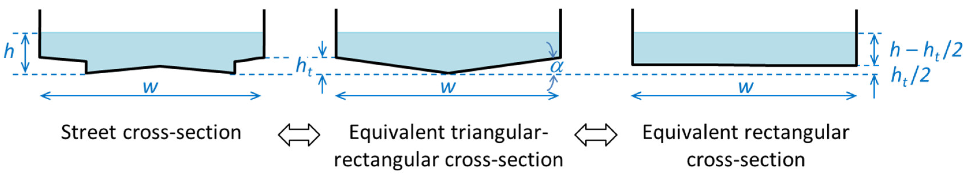
The cross-section shape of most streets is similar to the left-hand profile of Figure 1. This composite section and other variants can be represented, in a simpler way, by an equivalent triangular–rectangular cross-section, as shown in the profile at the center of Figure 1.

In this work, we will consider the flow in a triangular–rectangular cross-section, admitting a wide range of transversal slopes of the pavement on the triangular base ($\alpha$): from the null slope, which corresponds to a rectangular section, to a sufficiently high transversal slope, where the cross-section becomes triangular. This cross-section will be considered generic and representative of most streets.

The Manning–Strickler formula, valid for fully rough turbulent water flows, will be used:

$$V/\left(K.\sqrt{S}\right)=\mathrm{Q}/\left(K.\sqrt{S}\right)=R^{2/3}$$

(1)

where $V$ is the cross-section’s average velocity, $Q$ is the discharge, $K$ is the Strickler roughness value (the inverse of the Manning’s roughness, $n$), $S$ is the slope of the street bed, and $R$ is the hydraulic radius.

Only those situations where the width of the cross-section is significantly greater than the flow depth ($W\gg h$) will be considered. From a practical point of view, this happens for virtually all streets. This means that if the cross-section is rectangular, the hydraulic radius corresponds to the flow depth ($R\approx h$), and if the cross-section is triangular, the hydraulic radius corresponds to half the flow depth ($R\approx h/2$).

Consider a triangular–rectangular cross-section with triangular section depth $h_t$ and water depth $h$ above $h_t$ (the central profile of Figure 1). For $W\gg h$, it can be demonstrated that the flow rate and average flow velocity in that cross-section are equal to the flow rate and average velocity in a rectangular cross-section of the same width ($W$) and a depth equal to $h_{eq}=h-h_t/2$ (right-hand profile of Figure 1).

The concept of the equivalent rectangular cross-section will be used to quantify the effect of the variation of $h_t$ (i.e., the cross-section shape), together with the effects of the variation of the roughness and of the longitudinal slope of the street, in the compliance with the safety criteria. Condition $h.V\le limA$ will be designated by criterion A, and condition $h.V^2\le$ 1.23 m³s⁻² by criterion B. We should also consider the variable $X$, given by $X=K.\sqrt{S}$.

In the next section, the variation of $h$, $V$ and $Q/W$ for the thresholds of criteria A and B (with $limA$ ranging between 0.22 and 0.5 m²/s) are evaluated as a function of $h_t$ and $X=K.\sqrt{S}$. The discussion is carried out based on the equations that satisfy each criterion, and on the graphical results of those variations, which are valid for the supercritical flow. As the results for the triangular–rectangular cross-section are iterative, regression equations are obtained to easily compute $Q/W$ as a function of $h_t$ and $K.\sqrt{S}$. Thus, if the flood flow on a street is known, these equations allow us to determine expeditiously the minimum width of the street that fulfills the safety criteria.

In Section 4, this procedure is applied and tested in a case study tailored to cover a diverse set of situations, including subcritical and unsteady flows. Sensitivity analyses are also carried out for the shape and width of the cross-section of the streets, and for the roughness of both the street surfaces and the sewers.

3. Variation of h, V and Q/W Meeting the Thresholds of Criteria A and B as a Function of h_t and K.√S

3.1. Equations for the Thresholds of Criteria A and B

Considering $W\gg h$,

Table 1. Equations (adapted from [30]).

Criterion A: $\mathit{h}.\mathit{V}\le \mathit{l}\mathit{i}\mathit{m}\mathit{A}$m2/s	Rectangular cross-section	$h\le limA.{\left(K.\sqrt{S}\right)}^{-3/5}$	(2)
		$V\le lim{A}^{2/5}.{\left(K.\sqrt{S}\right)}^{3/5}$	(3)
		$Q/W\le limA$	(4)
	Triangular cross-section	$h\le lim{A}^{3/5}{.2}^{2/5}.{\left(K.\sqrt{S}\right)}^{-3/5}$	(5)
		$V\le lim{A}^{2/5}{.2}^{-2/5}.{\left(K.\sqrt{S}\right)}^{3/5}$	(6)
		$Q/W\le limA/2$	(7)
	Triangular–rectangular cross-section	Valid if $h_t\le lim{A}^{3/5}{.2}^{2/5}.{\left(K.\sqrt{S}\right)}^{-3/5}$	(8)
		Iterative calculation:
		$h\le limA.{\left(K.\sqrt{S}\right)}^{-1}.{\left(h-h_t/2\right)}^{-2/3}$	(9)
		$V\le limA/h$	(10)
		$Q/W\le limA.\left(h-h_t/2\right)/h$	(11)
		If Equation (8) is not valid (triangular flow):
		$Q/W\le lim{A}^{8/5}{.2}^{-3/5}.{\left(K.\sqrt{S}\right)}^{-3/5}.h_t{}^{-1}$	(12)
Criterion B: $\mathit{h}.{\mathit{V}}^{\mathbf{2}}\le \mathit{l}\mathit{i}\mathit{m}\mathit{B}$m3s−2	Rectangular cross-section	$h\le lim{B}^{3/7}.{\left(K.\sqrt{S}\right)}^{-6/7}$	(13)
		$V\le lim{B}^{2/7}.{\left(K.\sqrt{S}\right)}^{3/7}$	(14)
		$Q/W\le lim{B}^{5/7}.{\left(K.\sqrt{S}\right)}^{-3/7}$	(15)
	Triangular cross-section	$h\le lim{B}^{3/7}{.2}^{4/7}.{\left(K.\sqrt{S}\right)}^{-6/7}$	(16)
		$V\le lim{B}^{2/7}{.2}^{-2/7}.{\left(K.\sqrt{S}\right)}^{3/7}$	(17)
		$Q/W\le lim{B}^{5/7}{.2}^{-5/7}.{\left(K.\sqrt{S}\right)}^{-3/7}$	(18)
	Triangular–rectangular cross-section	Valid if $h_t\le lim{B}^{3/7}{.2}^{4/7}.{\left(K.\sqrt{S}\right)}^{-6/7}$	(19)
		Iterative calculation:
		${\left(K.\sqrt{S}\right)}^2.h.{\left(h-h_t/2\right)}^{4/3}\le limB$	(20)
		$V\le {\left(limB/h\right)}^{1/2}$	(21)
		$Q/W\le lim{B}^{1/2}.\left(h-h_t/2\right).h^{-1/2}$	(22)
		If Equation (19) is not valid (triangular flow):
		$Q/W\le lim{B}^{8/7}{.2}^{-1/7}.{\left(K.\sqrt{S}\right)}^{-9/7}.h_t{}^{-1}$	(23)
Simultaneity of criteria thresholds: $h.V=limA=0.5$ m2/s and $h.V^2=limB=1.23$ m3s−2	Rectangular cross-section	$Q/W=limA=0.5 {\mathrm{m}}^3{\mathrm{s}}^{-1}{\mathrm{m}}^{-1}$	(24)
		$K.\sqrt{S}=lim{B}^{5/3}.lim{A}^{-7/3}\approx 7.12 {\mathrm{m}}^{1/3}{\mathrm{s}}^{-1}$	(25)
		$h=lim{A}^2/limB\approx 0.203 \mathrm{m}$	(26)
		$V=limB/limA=2.460 \mathrm{m} {\mathrm{s}}^{-1}$	(27)
	Triangular cross-section	$Q/W=limA/2 {\mathrm{m}}^3{\mathrm{s}}^{-1}{\mathrm{m}}^{-1}$	(28)
		$K.\sqrt{S}=2^{2/3}.lim{B}^{5/3}.lim{A}^{-7/3}\approx 11.30 {\mathrm{m}}^{1/3}{\mathrm{s}}^{-1}$	(29)
		$h=lim{A}^2/limB\approx 0.203 \mathrm{m}$	(30)
		$V\approx limB/limA=2.460 \mathrm{m} {\mathrm{s}}^{-1}$	(31)
	Triangular–rectangular cross-section	$Q/W=limA-limB/limA.h_t/2$	(32)
		$K.\sqrt{S}=limB/limA.{\left(lim{A}^2/limB-h_t/2\right)}^{-2/3}=f\left(h_t\right)$	(33)
		$h=lim{A}^2/limB\approx 0.203 \mathrm{m}$	(34)
		$V=limB/limA=2.460 \mathrm{m} {\mathrm{s}}^{-1}$	(35)

presents the formulae for $h$, $V$ and $Q/W$ that verify each criterion for the rectangular, triangular and triangular–rectangular cross-sections (Equations (2)–(23)).

Criterion A ($h.V\le limA$) has the particularity that, for both the rectangular cross-section and the triangular one, the maximum flow per unit of width does not depend on $K.\sqrt{S}$. According to Equations (4) and (7), the threshold for $Q/W$ corresponds to the value of $limA$ for the rectangular cross-section, and to that of $limA/2$ for the triangular cross-section. For example, if $limA=$ 0.5 m²/s, then we have $Q/W\le$ 0.5 m³/s/m for the rectangular cross-section and $Q/W\le$ 0.25 m³/s/m for the triangular cross-section.

For both criteria, the calculation of the variables for the triangular–rectangular cross-section is iterative and only valid if one obtains $h\ge h_t$ (otherwise the cross-section is triangular). This check must be carried out before any iterative calculation, using Equation (8) for criterion A and Equation (19) for criterion B.

If the water height is higher than $h_t$, according to Equation (11) for criterion A, the threshold for $Q/W$ varies between $limA$ and $limA/2$ (in m³/s/m) depending on the quotient $\left(h-h_t/2\right)/h.$ This quotient corresponds to the ratio of the hydraulic radius of the equivalent rectangular cross-section with the calculated value of $h$. If the check shows that $h<h_t$, the values of $h$ and $V$ must be calculated considering the triangular cross-section, using Equations (5) and (6) for criterion A, and Equations (16) and (17) for criterion B. Because the width of the flow at the triangular base will be shorter than the width of the composite cross-section ($W$) in the ratio $h/h_t$, the maximum flow rate provided by Equations (7) and (18) must be multiplied by $h/h_t$, resulting the Equation (12) for criterion A and Equation (23) for criterion B.

3.2. Analytical Expressions for the Separation of the Relevant Criterion

Equations (24) to (35) in Table 1 result from solving the system of equations for criteria A and B, and the Manning–Strickler formula, also considering $W\gg h$.

Because neither $h_t$ or $X=K.\sqrt{S}$ are present in the equations for the calculation of $h$ and $V$ that verify both criteria, we conclude that the values of $h$ and $V$ that equate the thresholds of both criteria depend neither on the cross-section shape or on the roughness and slope of the street. According to Equations (26), (30) and (34) for $h$, and Equations (27), (31) and (35) for $V$, this happens for $h=lim{A}^2/limB$ and $V=limB/limA$, which correspond to $h\approx 0.203$ m and $V=$ 0.46 m/s for $limA=$ 0.5 m²/s and $limB=$ 1.23 m³s⁻².

However, $K.\sqrt{S}$ associated with this equality depends on the cross-section shape, as can be seen in the formula of Equation (33); it is $K.\sqrt{S}=lim{B}^{5/3}.lim{A}^{-7/3}\approx$ 7.12 m^1/3s⁻¹ for the rectangular cross-section (Equation (25)) and $K.\sqrt{S}=2^{2/3}.lim{B}^{5/3}.lim{A}^{-7/3}\approx$ 11.30 m^1/3s⁻¹ for the triangular cross-section (Equation (29)).

3.3. Graphical Results and Discussion

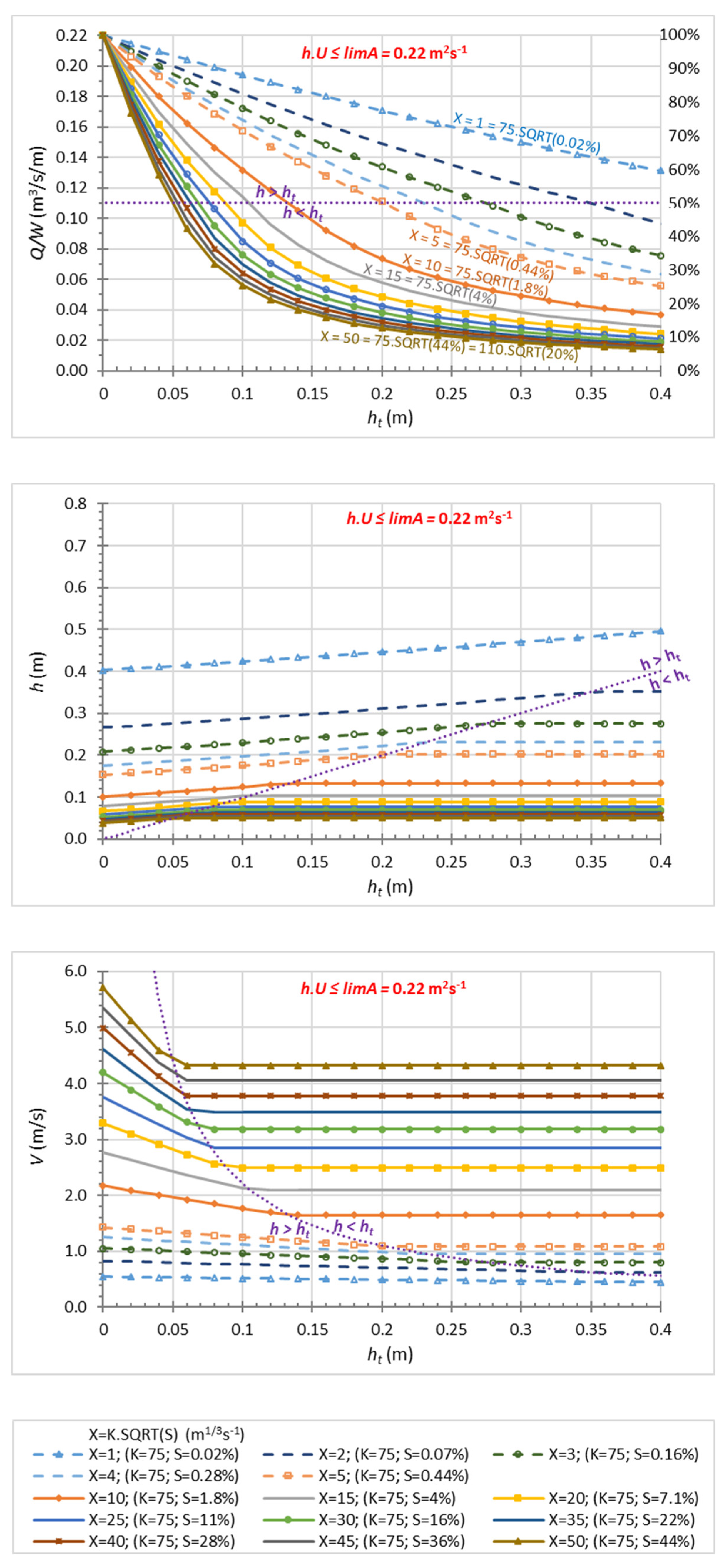
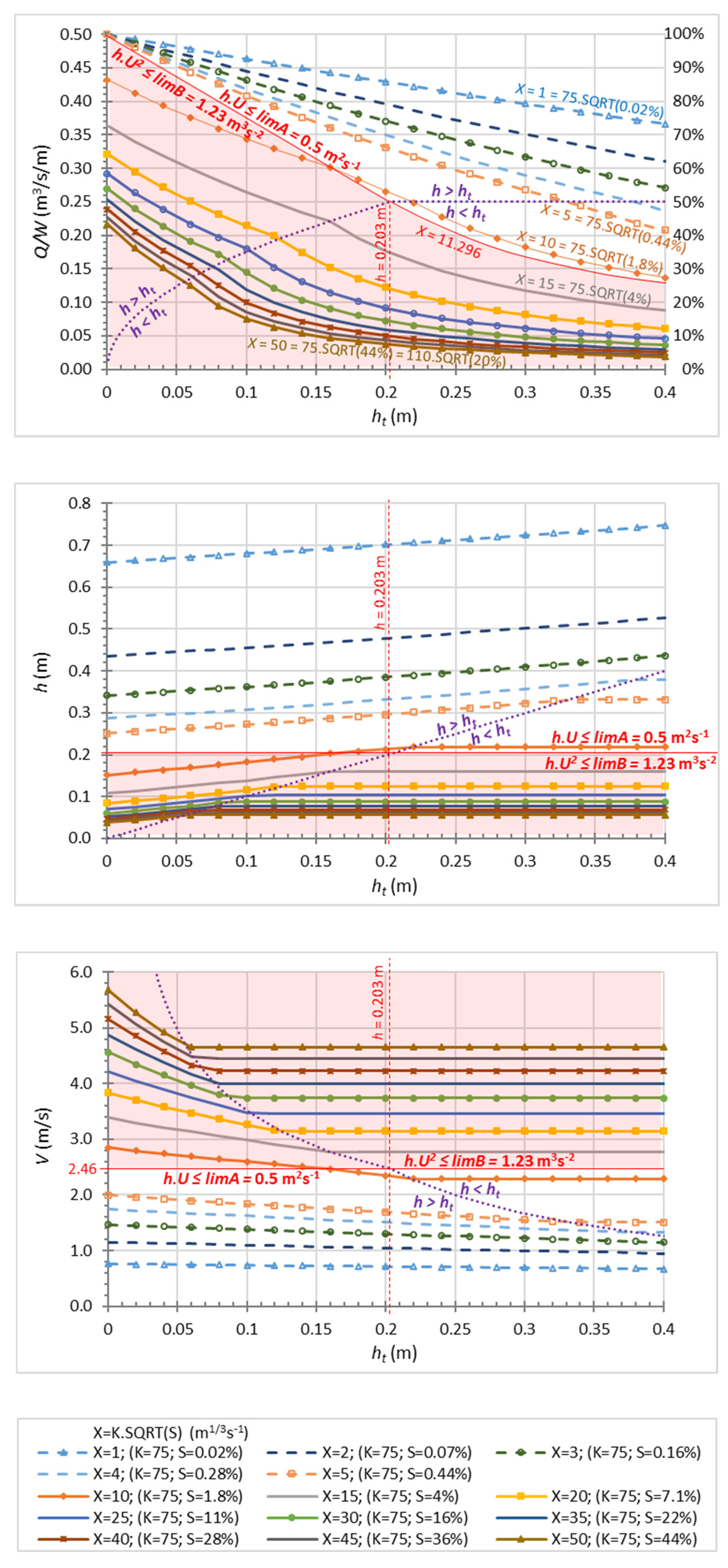
Figure 2 shows the variation of $Q/W$, $h$ and $V$ as a function of $h_t$ for different values of $K.\sqrt{S}$ and the adoption of criterion $h.V=$ 0.22 m²/s [18]. Figure 3 shows similar graphs, but now for the combination of criteria $h.V=$ 0.5 m²/s and $h.V^2\le$ 1.23 m³s⁻² [9,19].

The results on the y-axis of all of the graphs of Figure 2 and Figure 3 correspond to the particular case of the rectangular cross-section ($h_t=$ 0 m). In all of the graphs, the dotted line separates the flow in a triangular cross-section from the flow in the full triangular–rectangular cross-section (Equations (8) and (19) for $Q/W$). In Figure 3, the area where criterion B is determinant is shaded, which, as previously seen, corresponds to $h\ge$ 0.203 m, $V\le$ 2.46 m/s and $Q/W$ below the straight line of Equation (32) if $h_t\le$ 0.203 m, or $Q/W$ below the curve corresponding to $X=K.\sqrt{S}\approx$ 11.30 m^1/3s⁻¹ (Equation (29)) if $h_t\ge$ 0.203 m.

For both Figure 2 and Figure 3, the upper graphs show and allow us to quantify a significant reduction of $Q/W$ with the increase of $h_t$ and $X=K.\sqrt{S}$. For the case of the rectangular cross-section ($h_t=$ 0), $Q/W$ does not depend on $X=K.\sqrt{S}$ for condition A (as discussed earlier), but $Q/W$ can be significantly reduced with the increase of $X=K.\sqrt{S}$ due to criterion B (Figure 3). For example, for $h.V=$ 0.5 m²/s and a rectangular cross-section, we have $Q/W=$ 0.5 m³/s/m for all values of $K.\sqrt{S}\le$ 7.13 m^1/3s⁻¹ ($S\le$ 0.9% for $K=$ 75 m^1/3s⁻¹). However, for $K.\sqrt{S}=$ 15 m^1/3s⁻¹ ($S=$ 4% for $K=$ 75 m^1/3s⁻¹), $Q/W$ reduces to 0.36 m³/s/m for a rectangular cross-section due to criterion B, and for 0.18 m³/s/m for a triangular–rectangular cross-section with $h_t=$ 0.20 m (72% and 35% of 0.5 m³/s/m, respectively).

These results show that for steep streets, the maximum safety flows occur for small flow depths, usually below the sidewalks, and therefore are very sensitive to the resolution and quality of the topographic data. Thus, if high-resolution data are available and their treatment allows for the representation of the lower elevations next to the curbs, the results can be significantly more conservative than if this rigor is not considered.

However, streets with relatively constant average characteristics over tens of meters comprise extensive topographic variability in very detailed descriptions, due to various singularities (e.g., crossings, crosswalks, speed bumps, depressions near gutters and sinks). The detailed modelling of this variability will require great efforts in automatic calculation and result analysis, and it is very questionable whether the whole street design should be conditioned by the strict application of criteria A and B to small singularities, such as depressions next to the inlets. Furthermore, the use of high-resolution digital elevation models will introduce a large amount of information that will be treated as noise, aggravating data handling and computational requirements. The scaling effects of topographic variables and the advantages and disadvantages of using high-resolution digital elevation models for different purposes are discussed in more depth by [28,31].

3.4. Regression Equations for Iterative Q/W Values and the Proposal of an Expedited Method

The regression equations for $Q/W$ in the triangular–rectangular cross-section were obtained as a function of $h_t$ and $X=K.\sqrt{S}$. Equation (36) is valid for criterion A, considering the coefficients presented in

Table 2. Coefficients of the $Q/L$ regression equation for criterion A.

limA =	0.10 m2/s	0.22 m2/s	0.3 m2/s	0.4 m2/s	0.5 m2/s	0.22 m2/s ≤ limA ≤ 0.5 m2/s
a2 =	16.93	1.77	0.73	0.32	0.17	a2 = 0.023 limA−2.867
b1 =	31.26	5.46	2.75	1.45	0.89	b1 = 0.191 limA−2.214
b0 =	−8.28	−2.28	−1.37	−0.86	−0.59	b0 = −0.191 limA−1.637
c2 =	−0.0763	−0.0207	−0.0124	−0.0077	−0.0053	c2 = −0.0017∙limA−1.652
c1 =	7.3	2.10	0.81	0.81	0.57	c1 = 0.191∙limA−1.582
c0 =	15.38	4.61	1.85	1.85	1.32	c0 = 0.457 limA−1.527

(for $limA$ values equal to 0.1, 0.22, 0.3, 0.4 and 0.5 m²/s, or as a function of $limA$).

$$Q/W=1/\left(a_2.X^2.h_t{}^3+\left(b_1.X+b_0\right).h_t{}^2+\left(c_2.X^2+c_1.X+c_0\right).h_t+1/limA\right)$$

(36)

Equation (37) presents the regression equation for criterion B.

$$Q/W=1/\left(0.07.X^2.h_t^2+\left(0.011.X^2+0.36.X-0.07\right).h_t+0.86.X^{0.43}\right)$$

(37)

Equations (36) and (37) are valid for $h_t\le$ 0.5 m and 1 m^1/3s⁻¹ $\le X=K.\sqrt{S}\le$ 50 m^1/3s⁻¹.

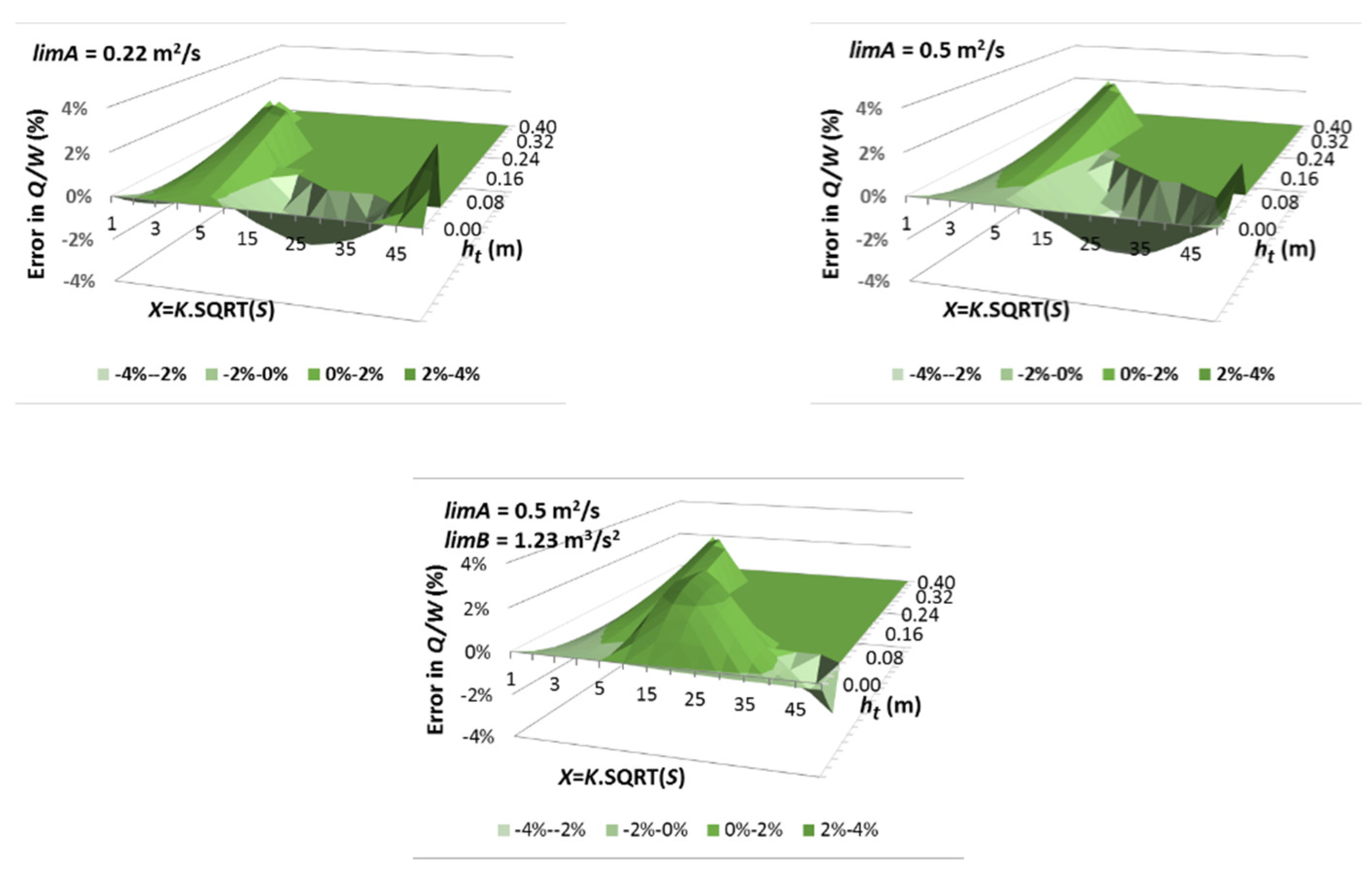
For the set of points shown in Figure 2 and Figure 3, the minimum and maximum errors obtained for all of the regressions based on Equations (36) and (37) and Table 2 were −3.1% and +3.2%, respectively. Figure 4 illustrates the errors obtained in the $Q/W$ estimates for $limA=$ 0.22 m²/s and $limA=$ 0.5 m²/s, and for the combination of $limA=$ 0.5 m²/s and $limB=$ 1.23 m³s⁻². In each graph, the flat area of null errors corresponds to the cases where $h\le h_t$.

Thus, $Q/W$ calculation can be easily implemented in a spreadsheet considering:

• Equation (36) or Equation (12), depending on Equation (8) for criterion A;
• Equation (37) or Equation (23), according to Equation (19) for criterion B.

With an estimate of the maximum flood flow rates obtained from more or less simplified models, these equations will provide the minimum street widths ($Wmin$) to meet safety criteria under supercritical flow conditions.

4. Case Study

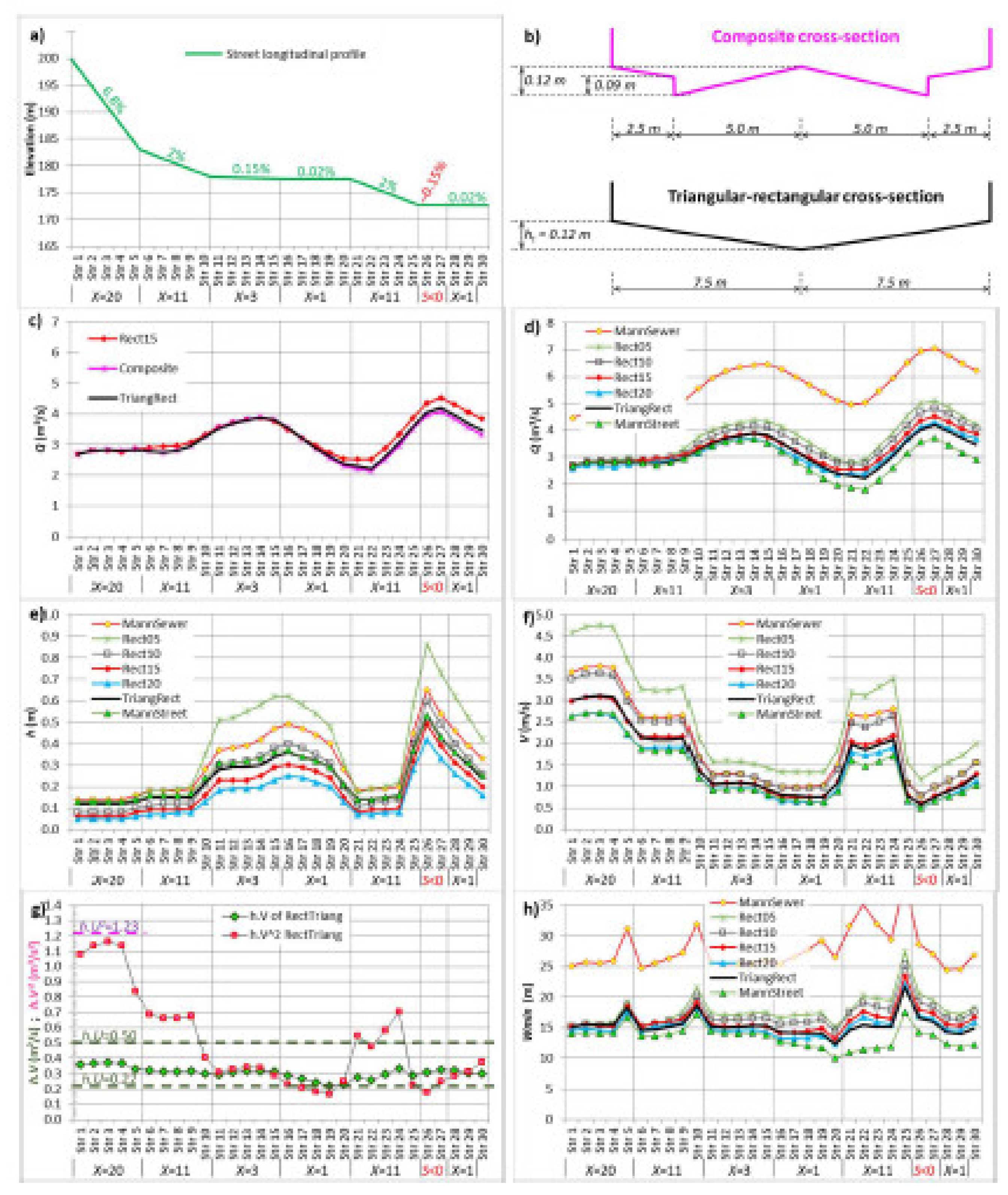
The approach proposed was applied to the dual drainage system represented in Figure 5, which was modelled using SWMM 5.1.011 [32]. The case study was built to assess the accumulated effect along a street of simplifications in the street cross-section, covering a diverse set of non-uniform unsteady flows, including subcritical flows. Simulations were run for a 100-year return period Desbordes hyetograph (a hyetograph composed of an increasing triangle, followed by a central peak and a decreasing triangle) and a recording interval of 1 minute. The street has 30 reaches of 50 m each, with different slopes and values of $X=K.\sqrt{S}$, as indicated in the table of Figure 5 (the Manning–Strickler coefficient was considered the same for all of the reaches of streets and sewers, $K=$ 1/0.013 $\approx$ 77 m^1/3s⁻¹). The changes in the slope of the reaches lead to alternating situations of supercritical and subcritical flows, and included a situation of negative slope in reaches 26 and 27. The cross-section of all of the street reaches was considered irregular, as shown in Figure 6b, with a maximum width of $W=$ 15 m. It can be approximated by a triangular–rectangular composite cross-section with $h_t=$ 0.12 m.

The sewer system receives runoff directly from an upstream 52-ha subcatchment, and from 26 subcatchments along the street with 0.5 ha each, representing the inflows from other sewers. The surface system receives runoff from 27 subcatchments along the street with 0.5 ha each. The flow transfers between the major and the minor system are ensured through 30 orifices with a diameter of 0.5 m each, representing the existence of approximately six inlets per reach. The upstream orifice has a larger diameter (2 m) in order to ensure the rapid balance between flows in the major system and in the minor system at the upstream boundary, and thus to guarantee numerical stability.

Figure 6c compares the maximum values of the flood flow ($Q$) recorded by SWMM in each reach for the following three street cross-sections: the composite section (“Composite”), the triangular–rectangular section (“TriangRect”), and the 15 m wide rectangular section (“Rect15”). The graph shows that the maximum flood flows of the triangular–rectangular cross-section are practically the same as those of the composite cross-section until about reach 19. Downstream of reach 19, the flow rate of the triangular–rectangular cross-section becomes slightly higher than that of the composite cross-section, increasing again a little further downstream of reach 27 (the reach with a negative slope). This very slight and progressive increase in the flow downstream is due to the fact that the area of the base of the triangular–rectangular cross-section is larger than the area of base of the composite cross-section. For the 15 m-wide rectangular cross-section, a similar behavior is observed, albeit with a more pronounced deviation downstream of reach 19. Some flow deviation is also observed in reaches 7 and 8 for the rectangular cross-section, which is recovered downstream.

Figure 6d–f compare the maximum values of $Q$, $h$ and $V$, respectively, for simulations using the triangular–rectangular cross-section (“TriangRect”) and the rectangular cross-sections with widths of 5, 10, 15 and 20 m (“Rect05”, “Rect10”, “Rect15”, “Rect20”). These Figures also show the results for the following two additional scenarios, considering the triangular–rectangular cross-section: a 20% decrease of the Strickler coefficient ($K$) in all streets (“MannStreet”), and a 20% decrease of $K$ in all sewers (“MannSewer”) (from $K=$ 1/0.013 $\approx$ 77 m^1/3s⁻¹ to $K=$ 1/0.01625 $\approx$ 61 77 m^1/3s⁻¹ for both cases).

For the purpose of this manuscript, it was ensured that $h>h_t=$ 0.12 m for the entire length of the street with a triangular–rectangular cross-section, as shown in Figure 6e. In the reaches with a negative slope, the flood depths reach 0.5 m, which would clearly necessitate the resizing of the downstream sewers if this were a real case. As expected, large differences in the $h$ and $V$ values are observed for the different cross-sections.

Figure 6d shows that for rectangular cross-sections with different widths from the triangular–rectangular cross-section (15 m), the results of $Q$ start to differ because of the first reaches, and that this difference is exacerbated downstream. The difference in the results increases with the difference in the width of the rectangular cross-section in relation to that of the triangular–rectangular cross-section.

The results in Figure 6d highlight that the roughness uncertainty has a more significant effect on the calculation of flood flows than the uncertainty in the shape of the cross-section. The 20% reduction in $K$ of the streets (“MannStreet”) leads to a significant reduction of the flood flows downstream (Figure 6d) due to the reduction of the flood velocities (Figure 6f). The 20% reduction in $K$ of the sewers (“MannSewer”) leads to increases of the flood flows that are much higher than all of the other scenarios. As with roughness, other factors that lead to changes in the transport capacity of the sewers, such as the sewer’s slope or diameter, also have a very significant influence on flood flows and, thus, on the fulfillment of the safety criteria.

Figure 6g shows the maximum values of $h.V$ and $h.V^2$ obtained in the successive reaches for the triangular–rectangular cross-section. All of the values of $h.V$ vary between circa 0.22 and 0.4 m²/s. In the upstream reaches, the $h.V^2$ values are close to but do not reach the 1.23 m³/s² threshold.

Based on the $h.V$ values presented in Figure 6g and the methodology presented in Section 3.4 of this manuscript, the minimum widths of the reaches ($Wmin$) were calculated as a function of the flow rates obtained for each simulation (Figure 6h). Figure 6h shows that, for the triangular–rectangular cross-section, the $Wmin$ results are close to 15 m in most reaches, both in supercritical and subcritical flows. However, in reaches 5, 10 and 25, the $Wmin$ values are significantly greater than 15 m. These three reaches have in common the fact that they are regime transition reaches, being midway between a significant increase of $h$ and a significant reduction of $V$. In reach 5, there is a transition from a supercritical to a slower supercritical flow, and in reaches 10 and 25 there is the transition from supercritical to subcritical flows. A slight oversizing of $Wmin$ is also observed in reaches 26 and 27, where the slope is contrary to the flow direction.

In practice, flow transitions that lead to hydraulic jumps should be avoided. In cases where there is a significant reduction in the street slope, the smoothing of the street slope reduction must be accompanied by a smoothing of the sewer transport capacity reduction in order to avoid an abrupt increase of floods downstream. At the crossing of a steep street with a flat perpendicular street, designing the street cross-section closer to the rectangular cross-section and capturing the runoff upstream of the crossing may be a solution.

In reach 20, the value of $Wmin$ for the triangular–rectangular cross-section is 12.5 m, about 17% less than 15 m. Reach 20 has a reduced slope, and is immediately upstream of a reach with a high slope. The passage through the critical flow in the transition must be the source of the lower value of $Wmin$. In reaches 16–19 and 28–29, $Wmin$ is slightly less than 15 m (in less than 5%). Part of this difference in the results is probably explained by the rounding to two decimal places of the results of $h$ and $V$. For the rectangular cross-sections, the $Wmin$ results reflect the flow deviations discussed with respect to Figure 6d.

5. Conclusions

The street’s cross-sectional profile plays a relevant role in meeting flood safety criteria, which is quantified and graphically described in this work. For example, a street with a 1.5% slope, $K\approx$ 75 m^1/3s⁻¹ and a rectangular cross-section complies with the threshold $h.V=$ 0.22 m²/s for twice the flow of a street with the same width but with a conventional cross-section shape and $h_t=$ 0.14 m. The flow will be four times greater for a 15% street slope (Figure 2).

However, the uncertainty associated with the data, models and results is generally significant, and should be taken into account in the compromise between detailing and simplifying the cross-sectional profile. The results of this manuscript confirm that, for various studies and projects of new developments, the consideration of equivalent triangular–rectangular cross-sections can lead to an adequate compromise between the quality of the data available and the calculation effort.

The results highlight that, on steeper streets, one way to increase the flood flow that meets the safety criteria is to approach the street cross-section to the rectangular section and catch the runoff through grated gutters in the full width of the street.

The approach presented in 3.4 can be used for the expedited verification of a street’s compliance with flood safety criteria. This approach allows for the calculation of the minimum width of the street ($Wmin$) based solely on the flood flow ($Q$). It is valid for most flows, except for rapidly varied flows.

The uncertainty of the street roughness can have a more significant effect on the flood flows, and thus on the fulfillment of the safety criteria, than the uncertainty of the street cross-section.

Finally, the case study highlighted that flood flows can vary exceptionally along the streets depending on the roughness, slope and diameter of the sewer system. During floods, surcharge and increased local head losses can significantly increase the average roughness of the sewer network, with high uncertainty. The existing deposits in the sewers and the dragging effects of mud, stones and debris during floods— which are generally calibrated for frequent storms—also increase the model’s uncertainty. The practical difficulty of representing and calibrating all of the flow transfer elements between the surface and the sewer models, and the current knowledge limitations in the parameterization of these devices, also contribute to raise uncertainty. These results emphasize that the effort in detailing the street’s cross-section must be framed with the objectives of the work and all of the sources of uncertainty.

References

- David, L.M.; Matos, J.S. Combined sewer overflow emissions to bathing waters in Portugal. How to reduce in densely urbanised areas? Water Sci. Technol. 2005, 52, 183–190. [Google Scholar] [CrossRef] [PubMed]
- Campisano, A.; Cabot Ple, J.; Muschalla, D.; Pleau, M.; Vanrolleghem, P.A. Potential and limitations of modern equipment for real time control of urban wastewater systems. Urban Water J. 2013, 10, 300–311. [Google Scholar] [CrossRef]
- Lund, N.S.V.; Falk, A.K.V.; Borup, M.; Madsen, H.; Mikkelsen, P.S. Model predictive control of urban drainage systems: A review and perspective towards smart real-time water management. Crit. Rev. Environ. Sci. Technol. 2018, 48, 279–339. [Google Scholar] [CrossRef]
- Demuzere, M.; Orru, K.; Heidrich, O.; Olazabal, E.; Geneletti, D.; Orru, H.; Bhave, A.G.; Mittal, N.; Feliu, E.; Faehnlej, M. Mitigating and adapting to climate change: Multi-functional and multi-scale assessment of green urban infrastructure. J. Environ. Manag. 2014, 146, 107–115. [Google Scholar] [CrossRef]
- Sörensen, J.; Persson, A.; Sternudd, C.; Aspegren, H.; Nilsson, J.; Nordström, J.; Jönsson, K.; Mottaghi, M.; Becker, P.; Pilesjö, P.; et al. Re-thinking urban flood management-time for a regime shift. Water 2016, 8, 332. [Google Scholar] [CrossRef] [Green Version]
- Stovin, V.R.; Moore, S.L.; Wall, M.; Ashley, R.M. The potential to retrofit sustainable drainage systems to address combined sewer overflow discharges in the Thames Tideway catchment. Water Environ. J. 2013, 27, 216–228. [Google Scholar] [CrossRef] [Green Version]
- Barbosa, A.E.; Fernandes, J.N.; David, L.M. Key issues for sustainable urban stormwater management. Water Res. 2012, 46, 6787–6798. [Google Scholar] [CrossRef]
- Hamel, P.; Daly, E.; Fletcher, T.D. Source-control stormwater management for mitigating the impacts of urbanisation on baseflow: A review. J. Hydrol. 2013, 485, 201–211. [Google Scholar] [CrossRef]
- Balmforth, D.; Digman, C.; Kellagher, R.; Butler, D. Designing for Exceedance in Urban Drainage–Good Practice; CIRIA C635: London, UK, 2006. [Google Scholar]
- Section 3: Stormwater Management. In City of Lethbridge Design Standards 2016 Edition; City of Lethbridge: Lethbridge, AB, Canada, 2016; Available online: https://www.lethbridge.ca/Doing-Business/Planning-Development/Urban-Construction-Right-of-Way-Coordination/Documents/City%20of%20Lethbridge%202016%20Standards.pdf (accessed on 3 July 2019).
- Melbourne Water. Standards and Specifications. Design. General Guidance, Australia, 2015, Chapter General Approach to Drainage Systems and Chapter Floodway Safety Criteria. Available online: https://www.melbournewater.com.au/planning-and-building/developer-guides-and-resources/standards-and-specifications (accessed on 3 July 2019).
- Hammond, M.J.; Chen, A.S.; Djordjević, S.; Butler, D.; Mark, O. Urban flood impact assessment: A state-of-the-art review. Urban Water J. 2015, 12, 14–29. [Google Scholar] [CrossRef] [Green Version]
- Nahiduzzaman, K.M.; Aldosary, A.S.; Rahman, M.T. Flood induced vulnerability in strategic plan making process of Riyadh city. Habitat Int. 2015, 49, 375–385. [Google Scholar] [CrossRef]
- Salinas-Rodriguez, C.; Gersonius, B.; Zevenbergen, C.; Serrano, D.; Ashley, R. A Semi Risk-Based Approach for Managing Urban Drainage Systems under Extreme Rainfall. Water 2018, 10, 384. [Google Scholar] [CrossRef] [Green Version]
- Shand, T.D.; Cox, R.J.; Blacka, M.J. Development of Appropriate Criteria for the Safety and Stability of Persons and Vehicles in Floods. In Proceedings of the 34th IAHR Conference, Brisbane, Australia, 26 June–1 July 2011; p. 9. [Google Scholar]
- Russo, B.; Gómez, M.; Macchione, F. Pedestrian hazard criteria for flooded urban areas. Nat. Hazards 2013, 69, 251. [Google Scholar] [CrossRef]
- Chanson, H.; Brown, R. Stability of Individuals during Urban Inundations: What Should We Learn from Field Observations? Geosciences 2018, 8, 341. [Google Scholar] [CrossRef] [Green Version]
- Martínez-Gomariz, E.; Gómez, M.; Russo, B. Experimental study of the stability of pedestrians exposed to urban pluvial flooding. Nat. Hazards 2016, 82, 1259. [Google Scholar] [CrossRef] [Green Version]
- Nanía, L.; Gomez, M.; Dolz, J. Analysis of risk associated to the urban runoff. Case study: City of Mendoza, Argentina. In Global Solutions for Urban Drainage, Proceedings of the 9th ICUD; Strecker, E.W., Huber, W.C., Eds.; ASCE: Reston, VA, USA, 2002. [Google Scholar] [CrossRef]
- Xia, J.; Falconer, R.A.; Wang, Y.; Xiao, X. New criterion for the stability of a human body in floodwaters. J. Hydraul. Res. 2014, 52, 93–104. [Google Scholar] [CrossRef] [Green Version]
- Shand, T.D.; Cox, R.J.; Blacka, M.J.; Smiths, G.P. Australian Rainfall and Runoff. Revision Projects. Project 10: Appropriate Safety Criteria for Vehicles. Literature Review; AR&R Report Number P10/S2/020; Water Research Laboratory, The University of New South Wales: Sydney, NSW, Australia, February 2011. [Google Scholar]
- Xia, J.; Falconer, R.A.; Xiao, X.; Wang, Y. Criterion of vehicle stability in floodwaters based on theoretical and experimental studies. Nat. Hazards 2014, 70, 1619–1630. [Google Scholar] [CrossRef]
- Martínez-Gomariz, E.; Gómez, M.; Russo, B.; Djordjević, S. A new experiments-based methodology to define the stability threshold for any vehicle exposed to flooding. Urban Water J. 2017, 14, 930–939. [Google Scholar] [CrossRef]
- Krebs, G.; Kokkonen, T.; Valtanen, M.; Setälä, H.; Koivusalo, H. Spatial resolution considerations for urban hydrological modelling. J. Hydrol. 2014, 512, 482–497. [Google Scholar] [CrossRef]
- Carvalho, R.F.; Lopes, P.; Leandro, J.; David, L.M. Numerical Research of Flows into Gullies with Different Outlet Locations. Water 2019, 11, 794. [Google Scholar] [CrossRef] [Green Version]
- David, L.M.; Carvalho, R.F.; Isidro, R.; Sobral, M. Stormwater control of new urban developments–Planning and modelling the Penalva system. In Proceedings of the 12th ICUD, Porto Alegre, Brazil, 11–16 September 2011; p. 8. [Google Scholar]
- Jahanbazi, M.; Egger, U. Application and comparison of two different dual drainage models to assess urban flooding. Urban Water J. 2014, 11, 584–595. [Google Scholar] [CrossRef]
- Leandro, J.; Djordjević, S.; Chen, A.S.; Savić, D.A.; Stanić, M. Calibration of a 1D/1D urban flood model using 1D/2D model results in the absence of field data. Water Sci. Technol. 2011, 64, 1016–1024. [Google Scholar] [CrossRef] [PubMed] [Green Version]
- Nanía, L.; León, A.; García, M. Hydrologic-Hydraulic Model for Simulating Dual Drainage and Flooding in Urban Areas: Application to a Catchment in the Metropolitan Area of Chicago. J. Hydrol. Eng. 2015, 20, 04014071. [Google Scholar] [CrossRef]
- David, L.M. Projetar para inundações–efeito do perfil, rugosidade e declive das ruas nos critérios de segurança. Águas Resíduos 2019, IV.4, 37–47. (In Portuguese) [Google Scholar] [CrossRef]
- Chang, K.T.; Merghadi, A.; Yunus, A.P.; Pham, B.T.; Dou, J. Evaluating scale effects of topographic variables in landslide susceptibility models using GIS-based machine learning techniques. Sci. Rep. 2019, 9, 12296. [Google Scholar] [CrossRef] [PubMed] [Green Version]
- Rossman, L.A. Storm Water Management Model User’s Manual Version 5.1; U.S. Environmental Protection Agency: Washington, DC, USA, 2015; EPA/600/R-14/413b. Revised September 2015.
Figure 1.
Street cross-section and equivalent cross-sections.
Figure 2.
Variations of , and fulfilling the thresholds of criterion m2s−1, as a function of and .
Figure 3.
Variations of , and fulfilling the thresholds of both criteria m2s−1 and m3s−2, as a function of and .
Figure 4.
Errors in the estimation of for 0.22 m2/s and 0.5 m2/s, and for the combination of 0.5 m2/s and 1.23 m3s−2.
Figure 5.
Map and longitudinal profile of the dual drainage system.
Figure 6.
Results from the case study: (a) Street longitudinal profile; (b) Dimensions of used composite and triangular-rectangular cross-sections; (c,d) flood maximum flows along the street; (e) flood maximum depths along the street; (f) flood maximum velocities along the street; (g) maximum values of criteria A and B along the street; (h) minimum street widths calculated by the expedited method as a function of the flow rates (actual width is 15 m).