Article

Glaciers and Paleorecords Tell Us How Atmospheric Circulation Changes and Successive Cooling Periods Occurred in the Fennoscandia during the Holocene

by
Jean-Louis Pinault
Independent Researcher, 96, Rue du Port David, 45370 Dry, France
J. Mar. Sci. Eng. 2021, 9(8), 832; https://doi.org/10.3390/jmse9080832
Submission received: 8 June 2021 / Revised: 27 July 2021 / Accepted: 29 July 2021 / Published: 31 July 2021
(This article belongs to the Special Issue Hydroclimatic Events in Regions Subject to Rainfall Oscillation)

Abstract

:
Two major climatic phenomena that occurred during the Holocene are interpreted from the resonance in subharmonic modes of long-period Rossby waves winding around the North Atlantic gyre, the so-called gyral Rossby waves (GRWs). These are, on the one hand, the change in atmospheric circulation that occurred in the North Atlantic in the middle Holocene, and, on the other hand, the occurrence of abrupt cooling events more frequently than what is generally accepted. The amplitude of GRWs is deduced by filtering, within bands characteristic of various subharmonic modes, climate records from the Greenland ice sheet, pollen, and tree rings in northern Fennoscandia, and from two Norwegian glaciers in northern Folgefonna and on the Lyngen peninsula. While the subharmonic modes reflect the acceleration/deceleration phases of the western boundary current, an anharmonic mode is evidenced in the 400–450 year band. Abrupt cooling events of the climate are paced by this anharmonic mode while the western boundary current is decelerating, and the northward heat advection of air favors the melting of the pack ice. Then, the current of the northernmost part of the North Atlantic gyre cools before branching off to the north, which alters its buoyancy. On the other hand, according to high subharmonic modes, high-pressure systems prevailed over the North Atlantic in the first half of the Holocene while low-pressure systems resulted from baroclinic instabilities of the atmosphere dominate during the second half, favoring the growth of glaciers in Scandinavia by a better snowfall in winter and cooler summers.

1. Introduction

1.1. The Climate System Is Subject to Long-Period Resonantly Forced Rossby Waves

The sensitivity of Arctic systems to climate changes during the Holocene is recognized as resulting from solar and orbital forcing [1]. However, the variations in solar insolation are too small to explain the observed transitions as simple linear responses. Likewise, the impact of volcanic eruptions on the climate system is too short to change it over very long periods of time. These reasons given are indicative of our ignorance of the mechanisms underlying climate variability. The causal relationships between the radiative forcing and the response of the climate system indeed reveal strong non-linearities that suggest resonance phenomena: the amplitude of the response of the climate system varies greatly depending on the period of forcing.
Positive feedback is indeed required to amplify the response of the climate system to external forcing. Here, climatic transitions will be interpreted as the response to orbital forcing of the climate system with the mediation of gyral Rossby waves (GRWs) propagating around the North Atlantic gyre [2]. They owe their existence to the gradient β of the Coriolis parameter relative to the mean radius of the gyre. Radiative forcing induces changes in the depth of the thermocline, and hence, the acceleration/deceleration of the modulated polar and radial currents around the gyre. The equations of motion of GRWs teach us that the modulated polar current is in phase with the oscillation of the thermocline while the modulated radial current is a quadrature ahead [3].
The mediation of GRWs is based on both observations and the properties of long-period Rossby waves that are approximately non-dispersive. The conceptualization of GRWs arises from the observation of the short-period Rossby waves that propagate where the western boundary current leaves the continent to re-enter the subtropical gyre. Propagating westward, these Rossby waves of a short period, less than or equal to 8 years, form progressive waves embedded into the wind-driven current of the gyre which flows eastward [4]. These baroclinic waves travel an apparent half-wavelength, then they escape from the gyre during the following half-period to merge with the poleward propagating drift current so that the poleward antinode is in opposite phase relative to the western antinode. Adjustment of the apparent wavelength to forcing conditions causes the Rossby waves to resonate under the effect of forcing by westerlies, of annual periodicity.
Likewise, long-period Rossby waves wind around the gyre for half a period, then escape from the gyre to propagate poleward. To do this, the Rossby wave, which propagates cyclonically, travels an integer number of turns around the gyre, embedded into the anticyclonic wind-driven current of the gyre, before escaping poleward. The GRW travels half an apparent wavelength around the gyre before leaving it so that the poleward antinode is in opposite phase relative to the antinode around the gyre. Here again, adjustment of the apparent wavelength to forcing conditions causes the Rossby waves to resonate under the effect of forcing resulting from the modulations of solar irradiance.
Due to the thermal gradient between the high and low latitudes of the gyre, acceleration/deceleration of the western boundary current induces variations in poleward transfer of heat. Consequently, acceleration of the western boundary current further deepens the thermocline which, in turn, accelerates the modulated polar current of the gyre even more as the thermal gradient is higher. This positive feedback loop causes a strong amplification of the response of the climate system to radiative forcing, the oscillation of the thermocline being approximately in phase with the forcing.

1.2. Subharmonic Modes

Multi-frequency GRWs overlap, behaving as coupled oscillators that share the same modulated polar current around the gyre. Consequently, GRWs are resonantly forced by solar and orbital cycles in subharmonic modes [4]. This means that each period is defined by recurrence. The first, the fundamental wave, is equal to 64 years. This is the apparent propagation time of the GRW around the North Atlantic gyre. The following periods are deducted from the period preceding them. To ensure optimum stability of the dynamic system, each period is double or triple the previous period. Each of the subharmonic numbers corresponds to the number of revolutions that the GRW travels during a period [5]. The first 11 subharmonic numbers are n 1 = 2 0 , n 2 = 2 1 , n 3 = 2 2 , n 4 = 3 × 2 2 , n 5 = 3 × 2 3 , n 6 = 3 × 2 4 , n 7 = 3 × 2 5 , n 8 = 3 × 2 6 , n 9 = 3 × 2 7 , n 10 = 3 × 2 8 , n 11 = 3 × 2 9 , whose periods are the product of the number of turns by 64, namely 64, 128, 256, 768, 1536, 3072, 6144, 12,288, 24,576, 49,152, and 98,304. The radiative forcing is even more efficient as the forcing period is closer to one of the natural periods of the GRWs.
The alternation of positive and negative sea surface temperature (SST) anomalies at high latitudes of the North Atlantic gyre results in the formation of low- or high-pressure systems stimulated by the polar jet stream [6,7]. The intensity of this ocean-atmosphere interaction, which is controlled by the amplitude of the modulation of the vertical temperature gradient in the subsurface seawater, depends on the various subharmonic modes. The surface temperature of the air over the North Atlantic deduced from proxies in the climate archives reflects the amplitude of GRWs when it is decomposed in subharmonic modes. Since the mid-Pleistocene transition (MPT), the amplitude of the subharmonic modes is subjected to the mode n 11 = 1536 whose period 98,304 years is remarkably close to the forcing period resulting from the variations in eccentricity [2]. This fundamental change in the behavior of glacial cycles during the quaternary glaciations occurred approximately 1.25–0.7 million years ago, in the Pleistocene epoch [8]. Before MPT, the fundamental period was 48 years, which means that the mode n 10 was tuned to variations in the obliquity, the forcing period of which is close to 41 Ka.
The amplitude of GRWs according to the subharmonic modes n 1 = 2 0 to n 11 essentially results from the energy transfer mechanisms between coupled oscillators, relayed by intermediate forcing when the forcing period is close to the natural period of one of the GRWs [5,9].

1.3. Evolution of Glaciers in the Northern Europe and the Climatic Transitions during the Holocene

As the extension of glaciers in Norway reacts quickly to the forcing of the climate system, their evolution offers opportunities to study climate variability during the Holocene [10]. In particular, the position of the equilibrium-line altitude (ELA) tightly reflects changes in temperature and precipitations over the North Atlantic [11,12]. The proportion of glacigenic material in sediments of glacier-fed lakes being positively correlated with glacier size, sediment yield may provide continuous records of glacier fluctuations, which is widely used in Scandinavia [13,14,15,16,17]. The decomposition of those climate records in subharmonic modes allows solving most of the mysteries surrounding the formation and evolution of these glaciers. Indeed, the evolution of glaciers in Fennoscandia according to high subharmonic numbers reflects the long-period phases of acceleration/deceleration of the western boundary current of the North Atlantic gyre, as will be seen further.
The aim of this work is to show how the evolution of glaciers reflects the subharmonic modes of the North Atlantic gyre, so that the mechanisms involved in teleconnections can be revealed, essentially the change in the atmospheric circulation over the North Atlantic from the mid-Holocene, then the successive abrupt cooling events that have occurred during the Holocene, including Bond events such as the Late Antique Little Ice Age (LALIA) and the Little Ice Age (LIA) [13,18,19,20]. In this case, it is the highlighting of an anharmonic mode that will make it possible to deepen the mechanisms which are responsible for them.

2. Materials and Methods

2.1. Data

The δ18O record obtained within the Greenland Ice Core Project (GRIP) is used as a proxy of global temperature in the northern hemisphere during the Holocene [21]; data are available at https://www.ncei.noaa.gov/pub/data/paleo/icecore/greenland/summit/grip/isotopes/gripd18o.txt.
The northern Fennoscandia 2000-year June–July temperature reconstruction [22] is available at ftp://ftp.ncdc.noaa.gov/pub/data/paleo/treering/reconstructions/europe/fennoscandia2014temperature.txt.
The Fennoscandia 7500-year pollen/tree-ring July temperature reconstruction [23] is available at ftp://ftp.ncdc.noaa.gov/pub/data/paleo/paleolimnology/europe/fennoscandia2012temperature.txt.
The Folgefonna, western Norway glacial lake sediment data and equilibrium-line altitudes (ELA) reconstruction [24] are available at https://www.ncei.noaa.gov/pub/data/paleo/paleolimnology/europe/norway/folgefonna2005.txt.
The northern Norway Aspvatnet glacial lake sediment data [25] are available at https://www.ncei.noaa.gov/pub/data/paleo/paleolimnology/europe/norway/aspvatnet2005.txt.

2.2. Filtering of Climatic Signals in Subharmonic Modes

Filtering chronologies in bands characteristic of subharmonic modes is performed by summing over a subset of the scales Morlet wavelet transforms. Morlet wavelet functions consist of a plane wave modulated by a Gaussian so that the scale and the period are confused [26]. The characteristic bands in which the filtering is performed according to the subharmonic numbers are given in [5,9].
Considering two adjacent bands, the filtered signal in the unified two bands is the sum of the filtered signals in each of the bands. In this way, the raw signal can be reconstructed from the sum of the filtered signals when the bands are representative of the whole spectrum of periods/frequencies. It can therefore be considered that the filtering is carried out without loss of information.

3. Results

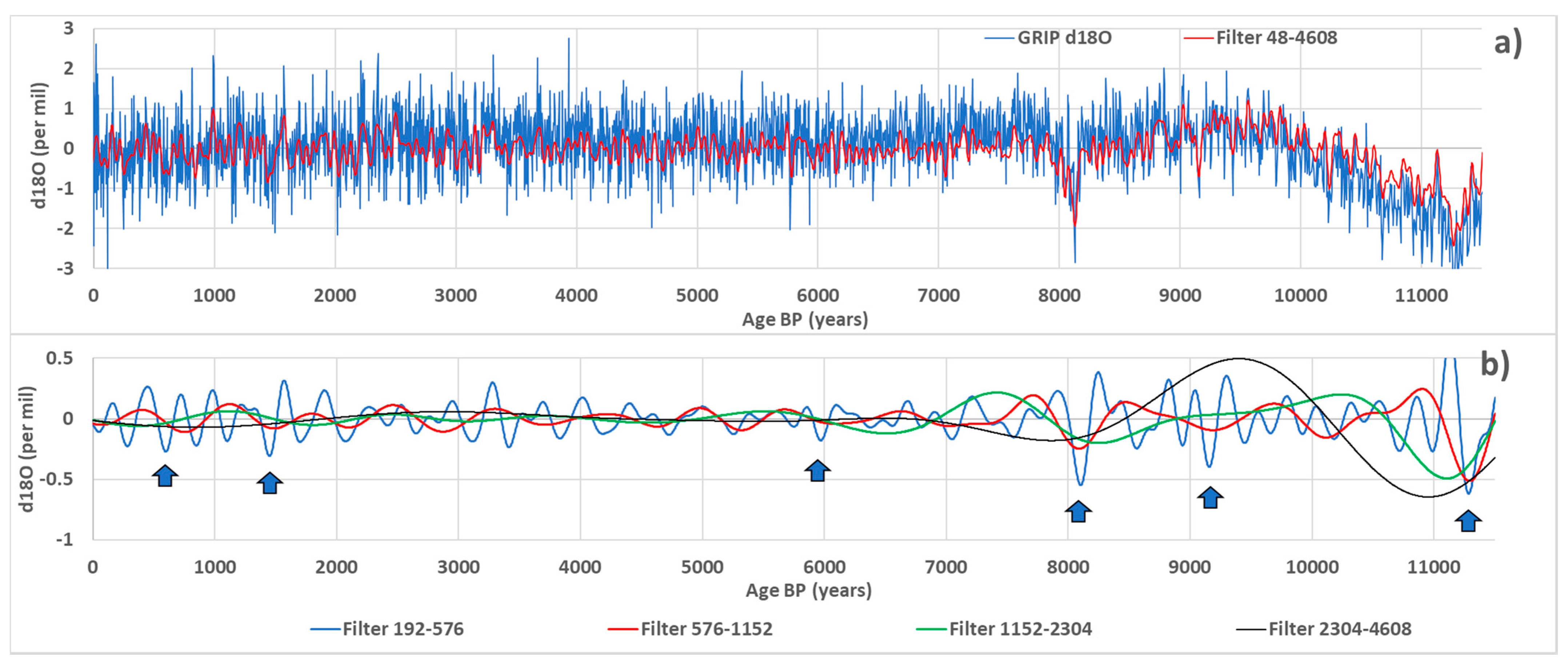
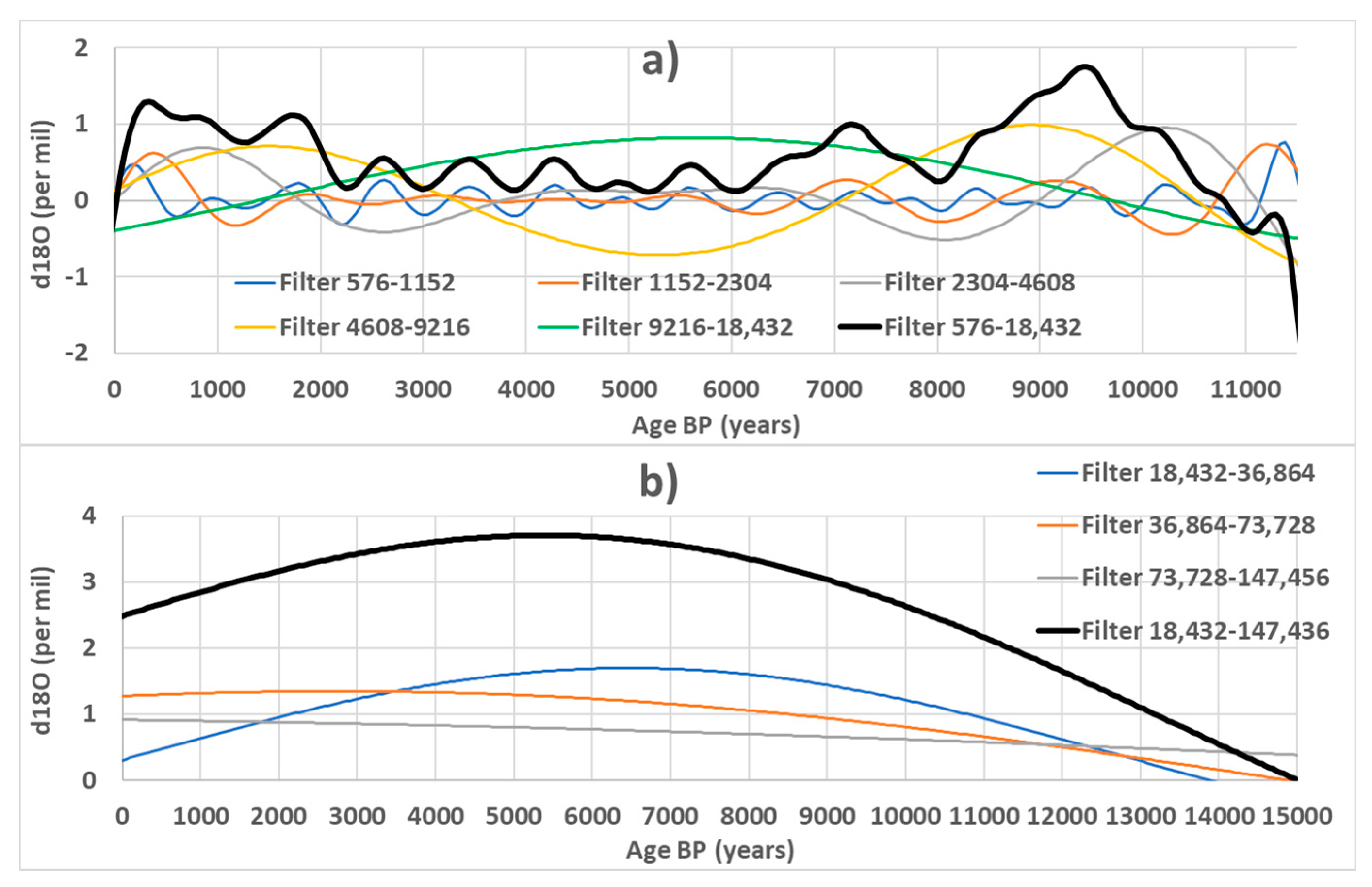
3.1. δ18O in GRIP Ice Core (Subharmonic Modes n 3 to n 6 )

The vast Greenland ice sheet [27] is an outstanding archive of past northern hemisphere atmospheric conditions. Among the ice core records sampled from this sheet, the Greenland ice core project (GRIP) provides an accurate proxy of global temperature during the Holocene from the concentration of δ18O in ice, with an effective resolution of a few decades [28].
In Figure 1a, the chronology is denoised from the sum of signals filtered in the characteristic bands of the subharmonic modes n 1 to n 6 . The signals referring to the subharmonic modes n 3 to n 6 are represented in Figure 1b. The oscillation of the mode n 6 that occurred in the early Holocene corresponds to the end of the ice age, showing a strong amplitude of the oscillation of the thermocline due to the large thermal gradient between the low and high latitudes of the gyre under the influence of still-extended pack ice. Damping of the GRW after 7000 yrs BP reflects a significant retreat of the pack ice.
The oscillation in the band 192–576 years plays a particular role in the early Holocene because three abrupt cooling events occurred nearly 8100, 9300, 11,300 yrs BP, at the minima of the filtered signal whose period is close to 400 years.

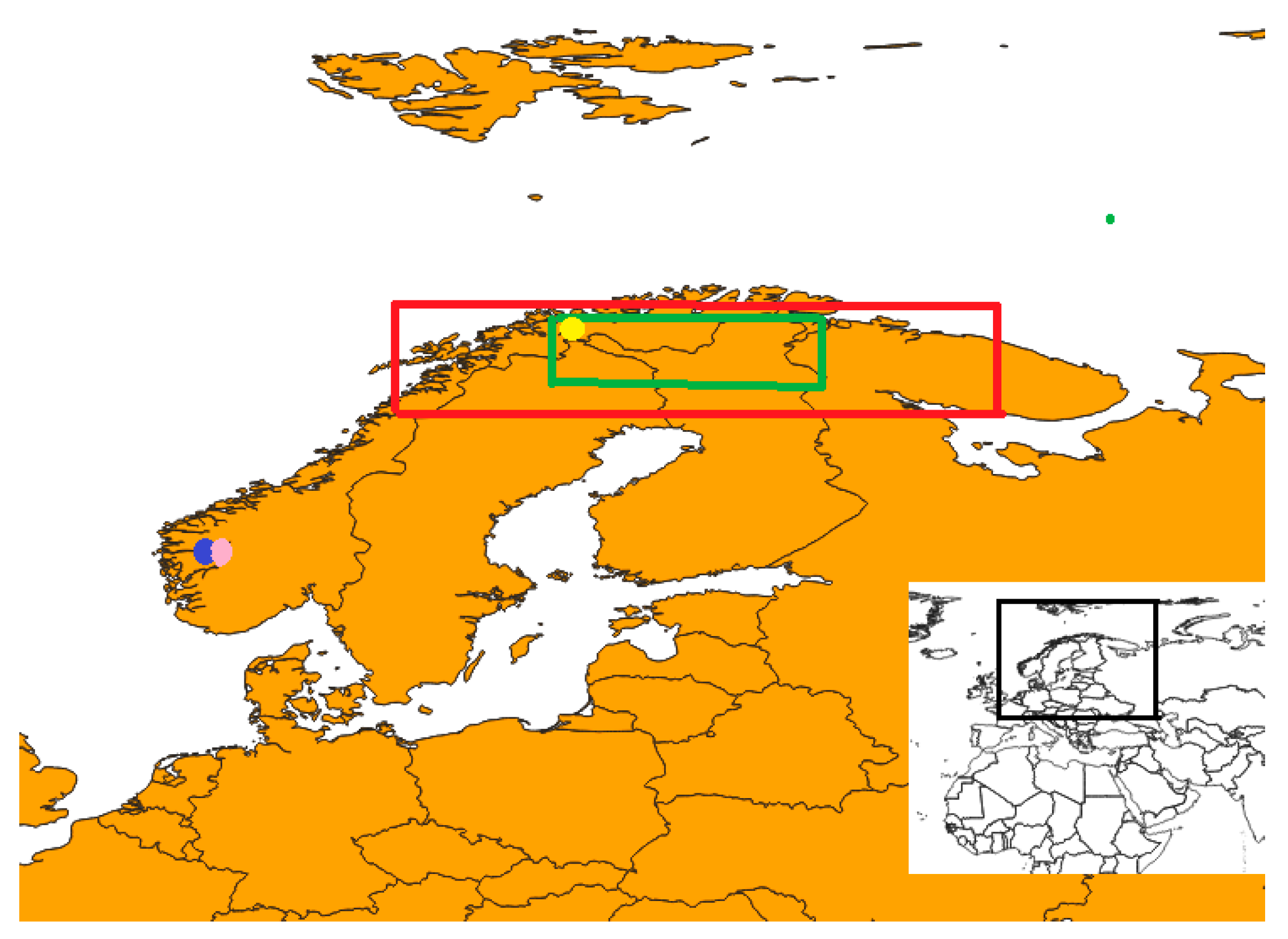
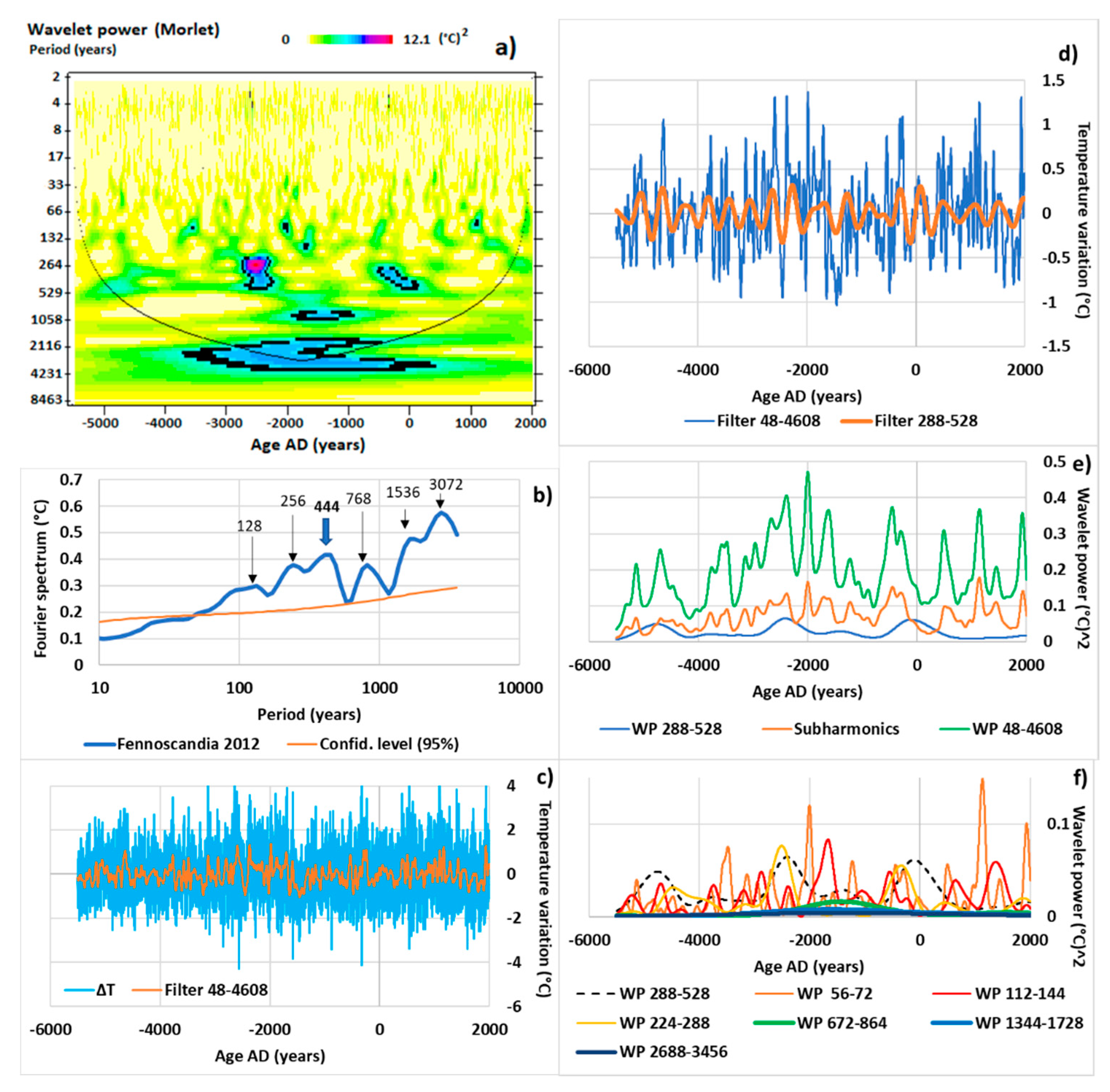
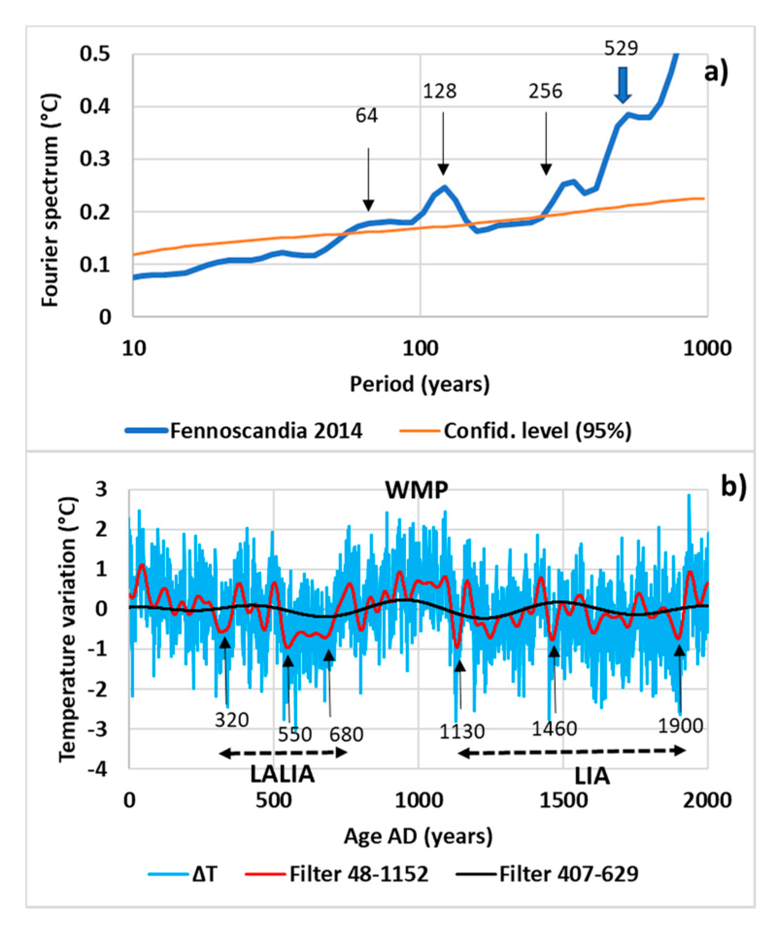
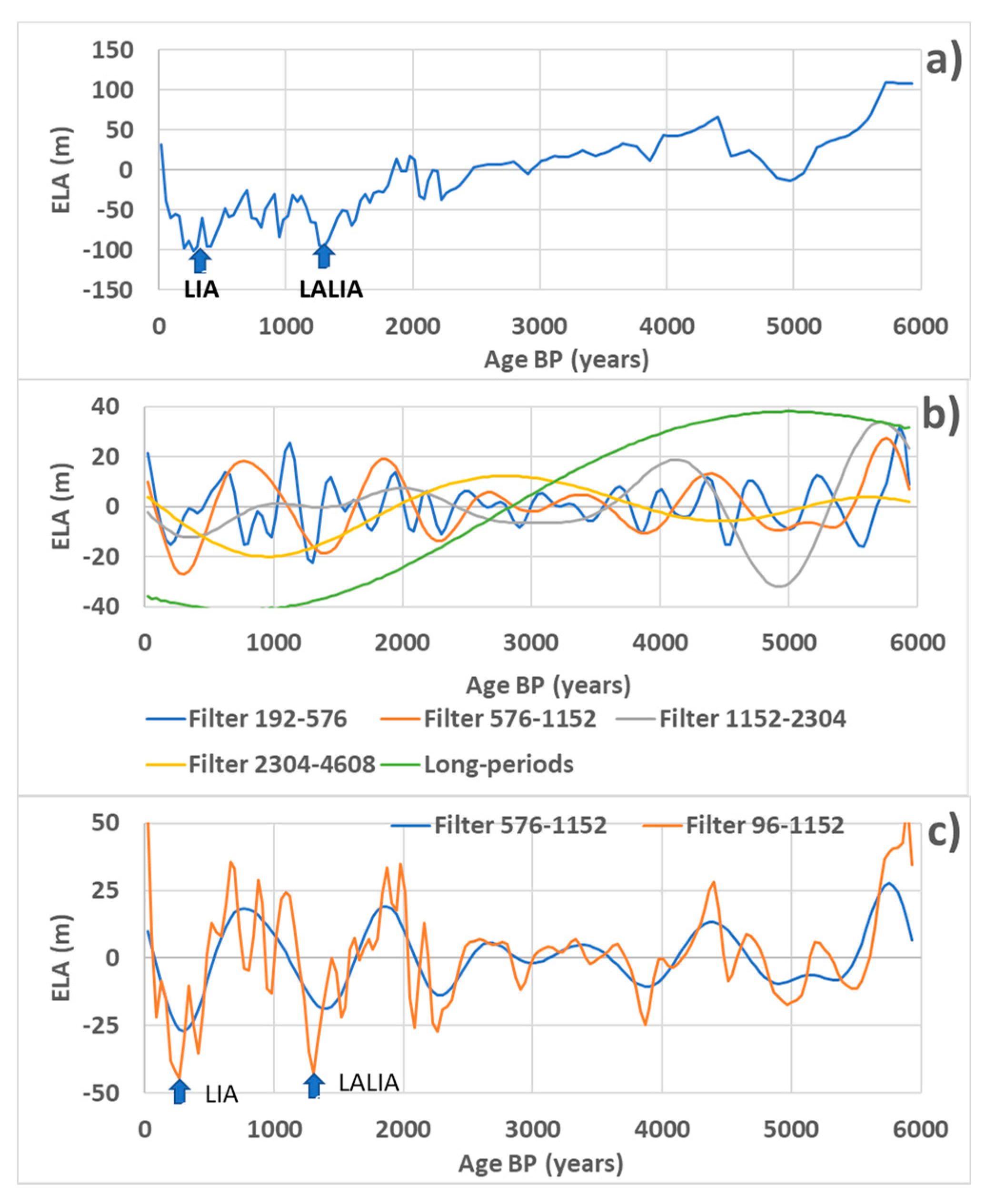
3.2. Tree-Rings and Pollen in Northern Fennoscandia

The northern Fennoscandia 2000-year June–July temperature reconstruction [22], and Fennoscandia 7500-year pollen/tree-ring July temperature reconstruction [23] provide annually resolved and absolutely dated proxies of global temperature from the mid-Holocene. The first chronology is based on a maximum latewood density of subfossil and modern tree-ring data whereas the second is based on pollen data from 11 lakes in northern Fennoscandia, plus July pollen/tree-ring data (Figure 2).
It emerges from the Fennoscandia 7500-years pollen/tree-ring July temperature reconstruction that the variability of the surface temperature is closely controlled by the subharmonic modes of the climate system. Indeed, the time-frequency wavelet power and the Fourier spectrum (the square root of the time-averaged wavelet power) of the chronology highlight five subharmonic modes, namely the modes n_2 to n_6 whose mean periods are 128, 256, 768, 1536, and 3072 years, respectively (Figure 3a,b). As a result, the climate of Fennoscandia faithfully reflects the phases of acceleration and deceleration of the western boundary current (the gulf stream) and the drift current of the North Atlantic subtropical gyre [3].
A broad, well-differentiated peak at the 444-year period indicates an anharmonic climate oscillation in the 288–528 year band. A relevant temporal resolution is obtained thanks, on the one hand, to the length of the chronology; on the other hand, the random errors affecting each year of observation can be likened to white noise. Thus, the process is decorrelated with a nearly zero autocorrelation R(Δt) at all points except at the origin: R(0) = 1.02, R(1) = 0.29, R(2) = 0.03, so that the incidence of random errors on the Fourier spectrum is very low for periods exceeding a few years (Figure 3b).
The northern Fennoscandia 2000-year June–July temperature reconstruction confirms that the long-term climate variations are dominated by subharmonic modes of the climate system (Figure 4a). The Fourier spectrum highlights the modes n_1 to n_3, the mean periods of which are 64, 128, and 256 years. The 2000 years of observation do not allow us to observe beyond that. On the other hand, the first mode appears here, although of low amplitude. Again, an anharmonic mode appears clearly in the Fourier spectrum, shifted compared to previous observations (mean period is 529 years). This shift, which is attributed to the shortness of the chronology compared to the period, is also observable for the subharmonic mode n_3. Here again, the anharmonic mode highlights successive cooling periods (signal filtered in the 407–629 year band), namely, the Little Ice Age (LIA) that mainly occurred in 1130, 1460 and in 1900 AD and the Last Antique Little Ice Age (LALIA) that occurred in 320 and in 550–680 AD, separated by the Medieval Warm Period (MWP): Figure 4b.

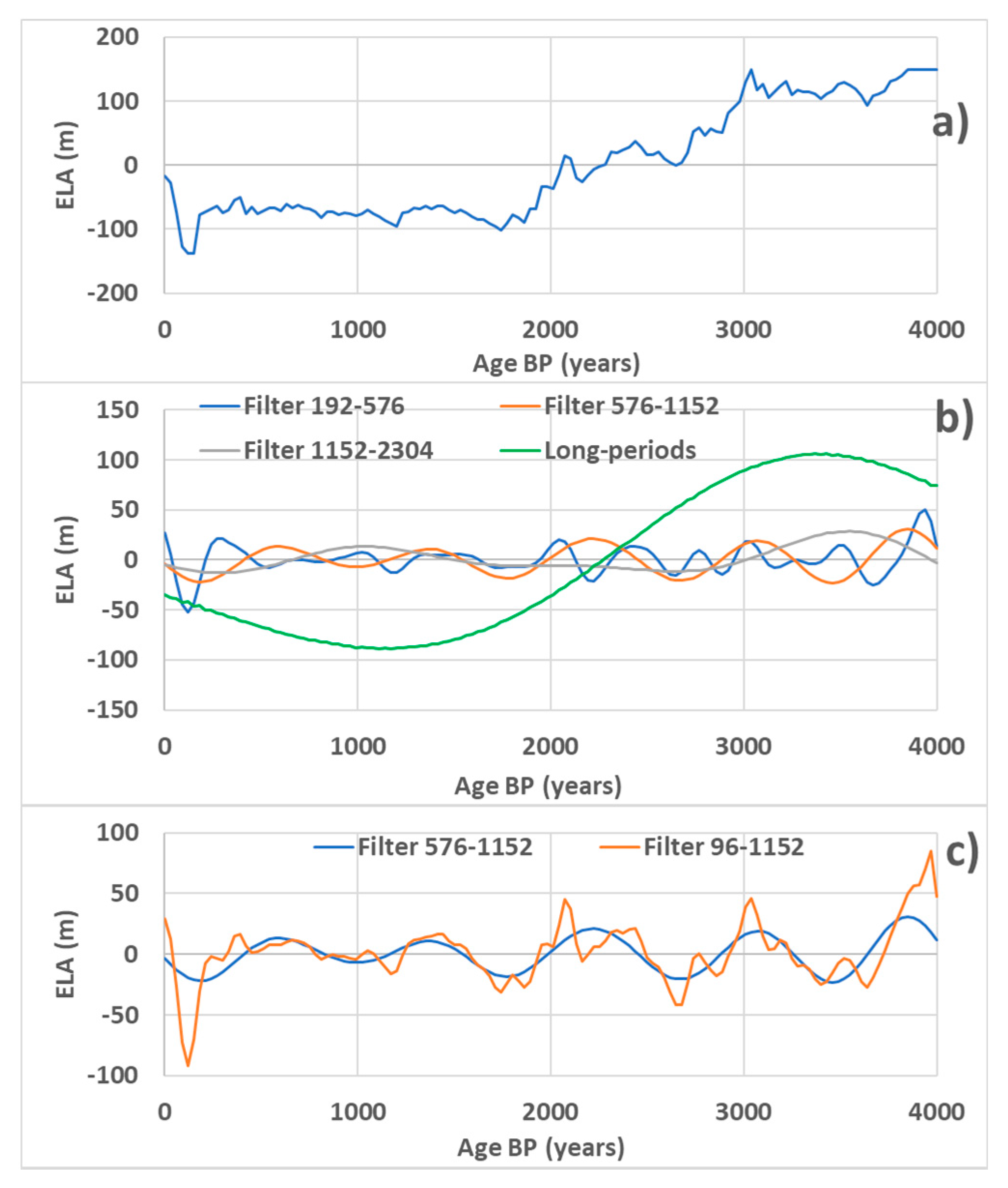
3.3. Glaciers in Norway

The regional temperature and precipitation patterns into the Norwegian Sea region are sensitive to variations of northward heat advection of air and water masses [25]. Fluctuations in glacier size and equilibrium-line altitude (ELA) are primarily the result of variations in summer temperature and/or winter precipitation as snow. Lacustrine and morpho-stratigraphical evidence allow obtaining detailed information concerning the size of glaciers over time [24,25].
When it is decomposed in subharmonic modes up to n 6 , imposed by the limitation of the length of the chronology, the ELA exhibits a low-frequency component characteristic of high subharmonic modes. Long periods are deduced from the difference between the raw signal and the sum of the components characteristic of the lower subharmonic numbers.
This low-frequency component shows that the two studied glaciers formed in the mid-Holocene, then extended steadily until they stopped growing before melting due to anthropogenic warming [24,25]. The size of the glacier in northern Folgefonna is determined with great precision since both the Little Ice Age (LIA) and the Last Antique Little Ice Age (LALIA) can be easily recognized (Figure 5). However, an integrating effect of the glacier merges the different cooling events occurring during LIA and LALIA into a single event. The formation of the glacier began around 6000 yrs BP with rapid growth followed by an episode of regression that lasted 1500 years. The size of the glacier on the Lyngen Peninsula shows that its formation began around 4000 yrs BP with steady growth that stopped 2000 yrs BP (Figure 6).
Here again, as concerns the high frequencies, the subharmonic mode n 4 is dominant during the whole live of the glaciers (Figure 5c and Figure 6c). Both have in common that they started growing in the mid-Holocene while the temperature in the northern hemisphere was relatively stable (Figure 1). This suggests a rapid change in atmospheric circulation which specifically affected the climate in northern Europe.

3.4. δ18O in GRIP Ice Core (Subharmonic Modes n 4 to n 11 )

The evolution of GRWs during the Holocene according to high subharmonic modes can only be understood by implying a global temperature signal extended to several tens of thousands of years of observation. Figure 7 shows the result of various filters applied to the proxy δ18O in GRIP ice core over 250,000 years (only the interval of time covering the Holocene is represented in Figure 7).
In Figure 7a, changes in the amplitude of GRWs subjected to subharmonic modes n 4 to n 8 exhibit two warm periods during the early Holocene, namely between 11,000 and 8000 yrs BP, and weaker between 8000 and 6000 yrs BP. Another warm period started 2000 yrs BP to present.
The Figure 7b shows that the amplitude of GRWs subjected to subharmonic modes n 9 to n 11 increased during the early part of the Holocene, then slowly decreased until the present day.

4. Discussion

Based on the resonance of the North Atlantic GRWs in subharmonic modes, the climatic fingerprints held by the two Norwegian glaciers, by botanical paleorecords as well as by the Greenland ice sheet, allow to specify and explain two major climatic phenomena during the Holocene; it was the successive cooling events, the period of which is 400–450 years, as well as the change in atmospheric circulation in the north Atlantic during the mid-Holocene.

4.1. Anharmonic and Subharmonic Modes

Lowering of the thermocline results from the baroclinic waves surrounding the North Atlantic gyre according to specific subharmonic modes. This occurs concomitantly with an acceleration of the modulated polar current around the gyre, accentuated along the western boundary where the gulf stream flows. Since the MPT, under the effect of variation in the eccentricity, the resonant forcing of the mode n 11 , the natural period of which coincides exactly with the forcing period [2], induces energy transfers between the different GRWs of lower subharmonic numbers. These are relayed by various intermediate forcing modes resulting from the intrinsic variation of solar irradiance, of higher frequency, as happens for the mode n 4 . In this case, the strength of the coupling is less because the tuning between the broadband forcing frequency with the natural frequency of the mode n 4 is less sharp. Likewise, the modulation of obliquity induces a weak coupling with the mode n 10 since the MPT because of the significant deviation between both periods, 41 and 49 Ka, respectively. On the other hand, the forcing resulting from the modulation of precession whose period is nearly 25 Ka is intrinsically weak because of its low amplitude [5].
The warming of the North Atlantic gyre implies the cooling of the drift current because the northern antinodes of the GRWs are in opposite phase with the respective antinodes around the gyre. There follows a thermal inversion between the gyre and the drift current.
Alongside the subharmonic oscillations of the climate system, an anharmonic oscillation is observed, which occurs in a wide band, and which cannot be straightforwardly linked to the oscillations of the thermocline and the acceleration/deceleration phases of the western boundary current. This anharmonic oscillation, which increases the variability of the climate system mainly in Europe, is related to rapid transitions.

4.2. Abrupt Cooling during the Holocene

As shown in the Figure 3d, the anharmonic oscillation of the climate system in the 288–528 year band is in phase with the abrupt changes in the denoised surface temperature during the 7500 years of observation. It is therefore that the temperature variations induced by the anharmonic mode, and which are added to the variations induced by the set of subharmonic modes, amplify the climatic extremes. This is particularly sensitive about abrupt cooling events such as those that occurred nearly 4500- and 3500-years BP.
These results confirm and clarify what is observed from the ice cores. The mean period deduced from the number of cycles of the filtered temperature in the band 192–576 years is about 400 years (Figure 1b).
Obviously, abrupt cooling events are favored when the western boundary current is slowing down. Presumably, the current of the gyre in its northernmost part before branching off to the north increases its density so that it plunges under surface water, not very salty because of the progressive melting of the pack ice promoted by the northward heat advection of air. It follows a significant cooling of northern Europe. The current of the gyre resurfaces as soon as it warms up and thermal exchanges are restored between the ocean and the continents. These transitions are rapid because the density of the surface layer and the underlying current of the gyre remain close, which favors the overturning.
The time correlation that is observable in Figure 3e between the wavelet power scale-averaged in the 48–4608 year band and the sum of wavelet powers scale averaged in successive 56–72, 112–144, 224–288, 672–864, 1344–1728, and 2688–3456 year bands shows that the characteristic bands corresponding to the different subharmonic modes are wider than those used and must be considered as joint. The characteristic band of the anharmonic mode is also wider than that used in the timing filtering so that the anharmonic mode interferes with the subharmonic modes. The Figure 3f shows that the dominant modes of climate variability are both the anharmonic mode and the subharmonic modes n 1 , n 2 , and n 3 .

4.3. Formation and Growth of Glaciers from the Mid-Holocene

As shown in Figure 7b, deepening of the thermocline of the North Atlantic gyre from the mid-Holocene, a consequence of the acceleration of the western boundary current in the context of the modes n 9 to n 11 , i.e., within the band 18,432–147,436 yrs, means that, stimulated by the polar jet stream, the high-pressure systems prevailed in the first half of the Holocene while the low-pressure systems promoted by baroclinic instabilities of the atmosphere are dominant during the second half. The conjunction of the cooling of the drift current and an increase in precipitation over northern and western Europe favors the growth of glaciers in Scandinavia due to more snowfall in winter and cooler summers.

5. Conclusions

Two major climatic phenomena were highlighted in Fennoscandia during the Holocene:
(1) Temperature reconstructions show that abrupt cooling events have occurred more frequently than is generally accepted, with an average period of 400–450 years and very variable periods and amplitudes. Resulting from an anharmonic oscillation of the climate system in northern Europe, they presumably reflect the cooling of the current of the northernmost part of the North Atlantic gyre. This causes a reduction in its buoyancy while the western boundary current is slowing down because of fresh water, resulting from melting of the pack ice promoted by the northward heat advection of air. Since LIA and LALIA are subjected to the anharmonic mode, it follows that these episodes are both the succession of two or three cooling events occurring during different cycles.
(2) The formation and extension of the two glaciers in northern Folgefonna and on the Lyngen Peninsula, Norway, which began at 6000 and 4000 yrs BP, respectively, highlight the change in atmospheric circulation that occurred during the middle Holocene. According to the resonance of GRWs in subharmonic modes n 9 to n 11 , the long-term acceleration of the gulf stream has resulted in a change in the prevalence of cyclones and anticyclones stimulated by the polar jet stream. In the north Atlantic, the highs prevailed during the first half of the Holocene, the lows during the second half.

Funding

This research received no external funding.

Data Availability Statement

Data sharing not applicable.

Acknowledgments

May the anonymous reviewers be generously thanked.

Conflicts of Interest

The authors declare no conflict of interest.

References

  1. Briner, J.P.; McKay, N.P.; Axford, Y.; Bennike, O.; Bradley, R.S.; de Vernal, A.; Fisher, D.; Francus, P.; Fréchette, B.; Gajewski, K.; et al. Holocene climate change in Arctic Canada and Greenland. Quat. Sci. Rev. 2016, 147, 340–364. [Google Scholar] [CrossRef] [Green Version]
  2. Pinault, J.L. Resonantly Forced Baroclinic Waves in the Oceans: A New Approach to Climate Variability. J. Mar. Sci. Eng. 2021, 9, 13. [Google Scholar] [CrossRef]
  3. Pinault, J.L. Modulated Response of Subtropical Gyres: Positive Feedback Loop, Subharmonic Modes, Resonant Solar and Orbital Forcing. J. Mar. Sci. Eng. 2018, 6, 107. [Google Scholar] [CrossRef] [Green Version]
  4. Pinault, J.L. Resonantly Forced Baroclinic Waves in the Oceans: Subharmonic Modes. J. Mar. Sci. Eng. 2018, 6, 78. [Google Scholar] [CrossRef] [Green Version]
  5. Pinault, J.L. Resonant Forcing of the Climate System in Subharmonic Modes. J. Mar. Sci. Eng. 2020, 8, 60. [Google Scholar] [CrossRef] [Green Version]
  6. Pinault, J.L. Regions Subject to Rainfall Oscillation in the 5–10 Year Band. Climate 2018, 6, 2. [Google Scholar] [CrossRef] [Green Version]
  7. Pinault, J.L. Global warming and rainfall oscillation in the 5–10 year band in Western Europe and Eastern North America. Clim. Chang. 2012, 114, 621–650. [Google Scholar] [CrossRef]
  8. Clark, P.U.; Archer, D.; Pollard, D.; Blum, J.D.; Rial, J.A.; Brovkin, V.; Mix, A.C.; Pisias, N.G.; Roy, M. The middle Pleistocene transition: Characteristics, mechanisms, and implications for long-term changes in atmospheric pCO2. Quat. Sci. Rev. 2006, 25, 3150–3184. [Google Scholar] [CrossRef] [Green Version]
  9. Explain with Realism Climate Variability. Available online: http://climatorealist.neowordpress.fr/subharmonic-modes/ (accessed on 2 April 2021).
  10. Dahl, S.O.; Bakke, J.; Lie, O.; Nesje, A. Reconstruction of former glacier equilibrium-line altitudes based on proglacial sites: An evaluation of approaches and selection of sites. Quat. Sci. Rev. 2003, 22, 275–287. [Google Scholar] [CrossRef] [Green Version]
  11. Sutherland, D. Modern glacier characteristics as a basis for inferring former climates with particular reference to the Loch Lomond stadial. Quat. Sci. Rev. 1984, 3, 291–309. [Google Scholar] [CrossRef]
  12. Dyurgerov, M. Glacier Mass Balance and Regime: Data of Measurements and Analysis; Meier, M., Armstrong, R., Eds.; Occasional Paper No. 55; Institute of Arctic and Alpine Research, University of Colorado: Boulder, CO, USA, 2002; pp. 10–15. [Google Scholar]
  13. Karle’n, W. Lacustrine sediments and tree-line variations as indicators of climatic fluctuations in Lappland, Northern Sweden. Geogr. Ann. 1976, 58, 1–34. [Google Scholar] [CrossRef]
  14. Nesje, A.; Matthews, J.A.; Dahl, S.O.; Berrisford, M.S.; Andersson, C. Holocene glacier fluctuations of Flatebreen and winter-precipitation changes in the Jostedalsbreen region, western Norway: Evidence from pro-glacial lacustrine sediment records. Holocene 2001, 11, 267–280. [Google Scholar] [CrossRef]
  15. Snowball, I.F.; Sandgren, P. Lake sediment studies of Holocene glacial activity in the Karsa valley, northern Sweden: Contrasts in interpretation. Holocene 1996, 6, 367–372. [Google Scholar] [CrossRef]
  16. Matthews, J.A.; Dahl, S.O.; Nesje, A.; Berrisford, M.S.; Andersson, C. Holocene glacier variations in central Jotunheimen, southern Norway, based on distal glaciolacustrine sediment cores. Quat. Sci. Rev. 2000, 19, 1625–1647. [Google Scholar] [CrossRef]
  17. Rosqvist, G.C.; Jonsson, C.; Yam, R.; Karle´n, W.; Shemesh, A. Diatom oxygen isotopes in pro-glacial lake sediments from northern Sweden: A 5000-year record of atmospheric circulation. Quat. Sci. Rev. 2004, 23, 851–859. [Google Scholar] [CrossRef]
  18. Giamali, C.; Koskeridou, E.; Antonarakou, A.; Ioakim, C.; Kontakiotis, G.; Karageorgis, A.P.; Roussakis, G.; Karakitsios, V. Multiproxy ecosystem response of abrupt Holocene climatic changes in the northeastern Mediterranean sedimentary archive and hydrologic regime. Quat. Res. 2019, 92, 665–685. [Google Scholar] [CrossRef]
  19. Bond, G.; Showers, W.; Cheseby, M.; Lotti, R.; Almasi, P.; de Menocal, P.; Priore, P.; Cullen, H.; Hadjas, I.; Bonani, G. A pervasive millennial scale cycle in North Atlantic Holocene and glacial climates. Science 1997, 278, 1257–1266. [Google Scholar] [CrossRef]
  20. Bond, G.; Kromer, B.; Beer, J.; Muscheler, R.; Evans, M.N.; Showers, W.; Hoffmann, S.; Lotti-Bond, R.; Hajdas, I.; Bonani, G. Persistent solar influence on North Atlantic climate during the Holocene. Science 2001, 294, 2130–2136. [Google Scholar] [CrossRef] [Green Version]
  21. Dansgaard, W.; Johnsen, S.J.; Clausen, H.B.; Dahl-Jensen, D.; Gundestrup, N.S.; Hammer, C.U.; Hvidberg, C.S.; Steffensen, J.P.; Sveinbjörnsdóttir, A.E.; Jouzel, J.; et al. Evidence for general instability of past climate from a 250 kyr ice-core record. Nature 1993, 264, 218–220. [Google Scholar] [CrossRef]
  22. Matskovsky, V.V.; Helama, S. Testing long-term summer temperature reconstruction based on maximum density chronologies obtained by reanalysis of tree-ring data sets from northernmost Sweden and Finland. Clim. Past 2014, 10, 1473–1487. [Google Scholar] [CrossRef] [Green Version]
  23. Helama, S.; Seppä, H.; Bjune, A.E.; Birks, H.J.B. Fusing pollen-stratigraphic and dendroclimatic proxy data to reconstruct summer temperature variability during the past 7.5 ka in subarctic Fennoscandia. J. Paleolimnol. 2012, 48, 275–286. [Google Scholar] [CrossRef]
  24. Bakke, J.; Lie, Ø.; Nesje, A.; Olaf Dahl, S.; Paasche, Ø. Utilizing physical sediment variability in glacier-fed lakes for continuous glacier reconstructions during the Holocene, northern Folgefonna, Western Norway. Holocene 2005, 15, 161–176. [Google Scholar] [CrossRef]
  25. Bakke, J.; Olaf Dahl, S.; Paasche, Ø.; Løvlie, R.; Nesje, A. Glacier fluctuations, equilibrium-line altitudes and palaeoclimate in Lyngen, northern Norway, during the Lateglacial and Holocene. Holocene 2005, 15, 518–540. [Google Scholar] [CrossRef]
  26. Torrence, C.; Compo, G.P. A practical guide for wavelet analysis. Bull. Am. Meteorol. Soc. 1998, 79, 61–78. [Google Scholar] [CrossRef] [Green Version]
  27. Vinther, B.; Clausen, H.B.; Johnsen, S.J.; Rasmussen, S.O.; Andersen, K.K.; Buchardt, S.L.; Dahl-Jensen, D.; Seierstad, I.K.; Siggaard-Andersen, M.-L.; Steffensen, J.P.; et al. A synchronized dating of three Greenland ice cores throughout the Holocene. J. Geophys. Res. 2006, 111, D13102. [Google Scholar] [CrossRef]
  28. Johnsen, S.J.; Clausen, H.B.; Dansgaard, W.; Gundestrup, N.S.; Hammer, C.U.; Andersen, U.; Andersen, K.K.; Hvidberg, C.S.; Dahl-Jensen, D.; Steffensen, J.P.; et al. The d18O record along the Greenland Ice Core Project deep ice core and the problem of possible Eemian climatic instability. J. Geophys. Res. 1997, 102, 26397–26410. [Google Scholar] [CrossRef]
Figure 1. δ18O in GRIP ice core: (a) raw and filtered chronologies. A broad band is used to reconstruct the denoised chronology (sum of signals filtered in the bands 48–96, 96–192, 192–576, 576–1152, 1152–2304 and 2304–4608 years); (b) signals filtered in the 192–576, 576–1152, 1152–2304 and 2304–4608 year bands are characteristic of the subharmonic modes n 3 = 2 2 , n 4 = 3 × 2 2 , n 5 = 3 × 2 3 , n 6 = 3 × 2 4 (mean periods = 256, 768, 1536, and 3072 years). Blue arrows indicate Bond events at 610, 1450, 5970, 8100, 9150, and 11,260 years BP.
Jmse 09 00832 g001
Figure 2. Location of glaciers and sampling areas of paleoproxies in Fennoscandia. Pollen data from 11 lakes, plus July pollen/tree-ring data for the past 7500 years [23] have been obtained in the red rectangle. Maximum latewood density of subfossil and modern tree rings data for the past 2000 years [22] have been obtained in the green rectangle. Western Norway glacial lake sediment data used to reconstruct ELA [24] have been obtained from the lakes Dravladalsvatn (blue circle) and Vassdalsvatn (pink circle). Sediment data from Aspvatnet glacial lake [25], Lyngen Peninsula, have been obtained in the yellow circle.
Jmse 09 00832 g002
Figure 3. Fennoscandia 7500-years July temperature reconstruction: (a) wavelet power and 95% confidence level; (b) Fourier spectrum; (c) raw and denoised (filtered in the 48–4608-year band) temperature variations; (d) temperature variations filtered in the 48–4608 and 288–528-year bands; (e) wavelet power (WP) scale-averaged in 288–528 and 48–4608-year bands. Subharmonics are the sum of wavelet powers scale averaged in 56–72, 112–144, 224–288, 672–864, 1344–1728, and 2688–3456 year bands; (f) components of the wavelet power scale-averaged in successive bands.
Jmse 09 00832 g003
Figure 4. Northern Fennoscandia 2000-years June–July temperature reconstruction; (a) Fourier spectrum and 95% confidence level; (b) raw and filtered temperature variation in the 48-1152 and 407–629 year bands.
Jmse 09 00832 g004
Figure 5. Equilibrium-line altitudes (ELA) of a glacier in northern Folgefonna, western Norway; (a) raw signal; (b) signal filtered in the characteristic bands of subharmonic modes n 3 = 2 2 , n 4 = 3 × 2 2 , n 5 = 3 × 2 3 , and n 6 = 3 × 2 4 (mean periods = 256, 768, 1536, and 3072 yrs) and the long-periods; (c) signal filtered in the band 576–1152 yrs characteristic of the subharmonic mode n 4 = 3 × 2 2 (mean period = 768 yrs), and in the band 96–1152 yrs, which includes the modes n 2 = 2 1 , n 3 = 2 2 , and n 4 = 3 × 2 2 (mean periods = 128, 256, and 768 yrs).
Jmse 09 00832 g005
Figure 6. Equilibrium-line altitudes (ELA) of a glacier on the Lyngen Peninsula, northern Norway; (a) raw signal; (b) signal filtered in the characteristic bands of subharmonic modes n 3 = 2 2 , n 4 = 3 × 2 2 , and n 5 = 3 × 2 3 (mean periods = 256, 768, and 1536 yrs) and the long periods; (c) signal filtered in the band 576–1152 yrs characteristic of the subharmonic mode n 4 = 3 × 2 2 (mean period = 768 yrs), and in the band 96–1152 yrs, which includes the modes n 2 = 2 1 , n 3 = 2 2 , and n 4 = 3 × 2 2 (mean periods = 128, 256, and 768 yrs).
Jmse 09 00832 g006
Figure 7. Long-period temperature signal obtained by filtering the proxy δ18O in GRIP ice core; (a) filters characteristic of the subharmonic modes n 4 = 3 × 2 2 , n 5 = 3 × 2 3 , n 6 = 3 × 2 4 , n 7 = 3 × 2 5 , and n 8 = 3 × 2 6 (mean periods = 768, 1536, 3072, 6144, and 12,288 yrs) and the sum (filter 576–18,432 yrs); (b) filters characteristic of the subharmonic modes n 9 = 3 × 2 7 , n 10 = 3 × 2 8 , and n 11 = 3 × 2 9 (mean periods = 24,576, 49,152, and 98,304 yrs) and the sum (filter 18,432–147,436 yrs).
Jmse 09 00832 g007
Publisher’s Note: MDPI stays neutral with regard to jurisdictional claims in published maps and institutional affiliations.

