
Evaluating the Effects of Sediment Transport on Pipe Flow Resistance


Department of Agricultural, Food and Forest Sciences, University of Palermo, Viale delle Scienze, Building 4, 90128 Palermo, Italy
*
Author to whom correspondence should be addressed.
Water 2021, 13(15), 2091; https://doi.org/10.3390/w13152091
Submission received: 15 July 2021
/
Revised: 28 July 2021
/
Accepted: 29 July 2021
/
Published: 30 July 2021
(This article belongs to the Section Hydraulics and Hydrodynamics)
Abstract
:In this paper, the applicability of a theoretical flow resistance law to sediment-laden flow in pipes is tested. At first, the incomplete self-similarity (ISS) theory is applied to deduce the velocity profile and the corresponding flow resistance law. Then the available database of measurements carried out by clear water and sediment-laden flows with sediments having a quasi-uniform sediment size and three different values of the mean particle diameter Dm (0.88 mm, 0.41 mm and 0.30 mm) are used to calibrate the Γ parameter of the power-velocity profile. The fitting of the measured local velocity to the power distribution demonstrates that (i) for clear flow the exponent δ can be estimated by the equation of Castaing et al. and (ii) for the sediment-laden flows δ is related to the diameter Dm. A relationship for estimating the parameter Гv obtained by the power-velocity profile and that Гf of the flow resistance law is theoretically deduced. The relationship between the parameter Гv, the head loss per unit length and the pipe flow Froude number is also obtained by the available sediment-laden pipe flow data. Finally, the procedure to estimate the Darcy-Weisbach friction factor is tested by the available measurements.
1. Introduction
The sand-water mixture flow is affected by the physical properties of the fluid and the kind, size and concentration of the transported particles [1].
From a practical point of view, the process of transporting solids and liquid phases through closed pipes is widely applied and economic considerations support the employment of this method of transportation. Sediment transport through pipes is used in dredging process to remove sand, silt and other material from rivers, channels, watersheds, and harbors. Sewerage engineers use a self-cleaning velocity as that which allows to transport sediments in the flow without deposition processes on the sewer bed. Hydraulic transport is also widely applied to transport mine and quarry products. The characterization of sand particles’ transport in different flow systems, such as sand-multiphase mixtures, is very important to predict the sand transport velocity and entrainment processes in oil and gas transportation pipelines. A production system affected by sand should be designed to operate above the critical sand deposition velocity to assure that solid particles are dispersed in fluid phases [2].
Notwithstanding the numerous applications of the sediment transport through pipes, information about this process is inadequate and limits a rational approach to the design issues [3,4].
Friction factor evaluation for pipe sediment-laden flows is a theme to be discussed as a limited number of studies were conducted before [3,5]. Resistance of clear flows moving in rough pipes and fixed boundary channels can be certainly estimated. On the contrary, the assessment of flow resistance for sediment-laden flow moving in pipes is not completely solved.
Previous experiments on sand transport in pipes have been primarily concerned with dredging, which is characterized by suspended load moving at high velocities. When the velocity and the sediment concentration are relatively low, the major amount of sediments is transported near to the bottom and only a small percentage is carried in suspension [6].
Melisenda [5] carried out some experiments using a pipe having a diameter of 0.104 m and a total length of 80 m. The runs were carried out using both clear water and sediment-laden flows carrying sediments with a quasi-uniform sediment size and three different values of the mean diameter Dm (0.88 mm, 0.41 mm and 0.30 mm). The experimental pipe was equipped by a Venturi pipe and some pressure head gauges to measure flow discharge Q and pipe head losses. The local flow velocity distribution was measured in a diameter pipe using a Pitot tube. The measurements demonstrated that, in comparison with the clear flow conditions, (i) the effects of transported sediment particles are appreciable for the highest values of Dm and (ii) the differences in local flow velocity occur in the zone of the profile below the maximum velocity value.
In the study of uniform pipe flow, the theoretical deduction of the flow resistance law by integration of a known velocity profile in the cross-section is an actual task. In the past, for the clear flow condition, the incomplete knowledge of the flow velocity distribution supported the empirical analysis of pipe head loss measurements.
In a previous paper [7], for a uniform clear water turbulent flow in a smooth circular pipe, using the incomplete self-similarity hypothesis [8,9], the following power-velocity distribution was deduced:
in which v is the mean local velocity, y is the distance from the pipe wall, is the shear velocity, g is acceleration due to gravity, D is the pipe diameter, J is the head loss per unit length, νk is the kinematic viscosity, Г and δ are the scale factor and the exponent of the power velocity profile, respectively.
According to the studies of Castaing et al. [10], δ can be calculated using the following relationship:
in which Re is the Reynolds number equal to VD/νk, V is the mean flow velocity and δo is a constant which Barenblatt [11] estimated equal to 1.5 using the velocity data of Nikuradse [12,13]. The studies by Butera et al. [9] gave δo = 1.55 which was justified by the experimental installation and measurements technique different from those used by Nikuradse [12].
By integrating Equation (1), the following expression of the Darcy-Weisbach friction factor f is obtained [7,9]:
The applicability of Equation (3) was recently tested for uniform open channel flows having a suspended sediment load [14]. For sediment-laden flows, having known values of mean diameter and suspended sediment concentration, a relationship between the Γ parameter of Equation (1), the channel slope and the Froude number was calibrated by the available measurements. A relationship for estimating Г which considers the mean concentration of suspended particles was also obtained. For large-size mixtures, the Darcy–Weisbach friction factor can be estimated with accuracy even if the effect of mean suspended sediment concentration is negligible. For small-size mixtures, the friction factor decreases when the mean sediment concentration increases.
The main aim of this paper is to apply a theoretical flow resistance law (Equation (3)) for pipes in which sediment-laden flows are conveyed. The theoretical approach is supported by the available database of measurements carried out by clear water and sediment-laden flows with sediments having a quasi-uniform sediment size and three different values of the mean particle diameter Dm (0.88 mm, 0.41 mm and 0.30 mm) [5]. The velocity measurements are used to calibrate the δ exponent and the Γ parameter of the power-velocity profile. The estimate of Γ parameter, Γv, obtained by the power-velocity profile (Equation (1)) and that Γf deduced by the flow resistance law (Equation (3)) are theoretically related. Then a relationship between the parameter Гv, the head loss per unit length and the pipe flow Froude number is also obtained by the available sediment-laden pipe flow data. Finally, the procedure to estimate the Darcy-Weisbach friction factor is tested by the available measurements.
2. Materials and Methods
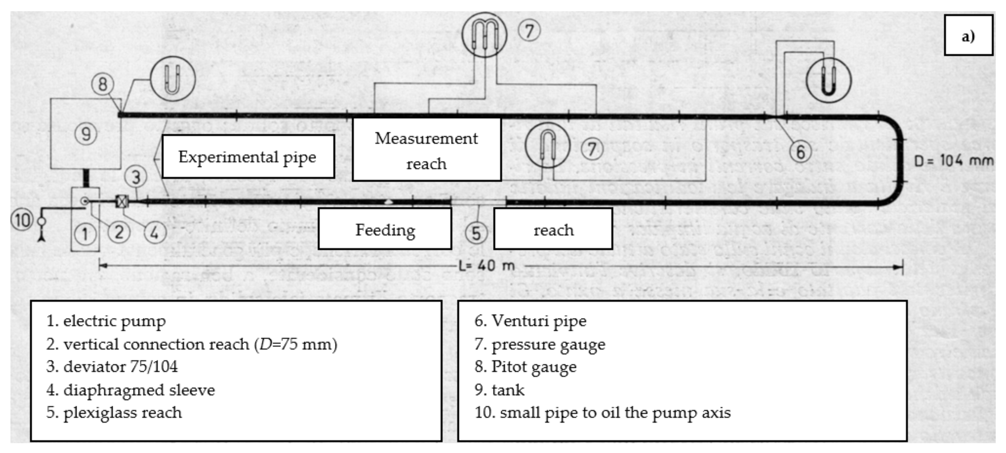
The experimental layout by Melisenda [5] was constituted of (i) an electric pump, able to pump a mixture of water and sand, (ii) the experimental pipe, having a pipe diameter D = 0.104 m, which was 80 m (a feeding reach and a measurement reach, each 40 m long) and (iii) a tank with a sand supply box to prepare the water-sand mixture (Figure 1a).
The feeding pipe was equipped with a discharge regulator and a plexiglass reach (Figure 1b) which allowed to control the sediment transport inside the pipe and to verify if sand deposition or bed-load transport occurred. The measurement pipe reach was equipped with a Venturi pipe to measure the discharge, and five pressure gauges to measure the head loss per unit length. The closed-circuit pipe ended within a tank and a Pitot gauge was installed in the cross-section 5 cm apart from the pipe end. The Pitot gauge allowed to measure the mean local velocity at a known distance from the pipe wall and was controlled by a position device which allowed to move the gauge along a diameter of the cross-section. Experiments were carried out for values of the sand concentration varying from 0 (clear water) to 0.0848. In this range of the volumetric concentration and for the investigated kinematic conditions, the sand was always suspended into the flow. The investigated flows were always turbulent (228,480 ≤ Re ≤ 540,293).
For investigating the clear flow condition, the measurements by Butera et al. [9] were also considered. Butera et al. [9] carried out their experiments using a horizontal plexiglass pipe, 11 m long and having a diameter D of 0.15 m. The discharge was measured by an electromagnetic flowmeter and the piezometric head was measured in seven cross-sections by piezometers. Twenty values of discharge, in the range 1.73–55.12 L s−1, were used. Moreover, for this database the investigated flows were always turbulent (14,161 ≤ Re ≤ 442,224).
3. Results
3.1. Flow Velocity Profiles
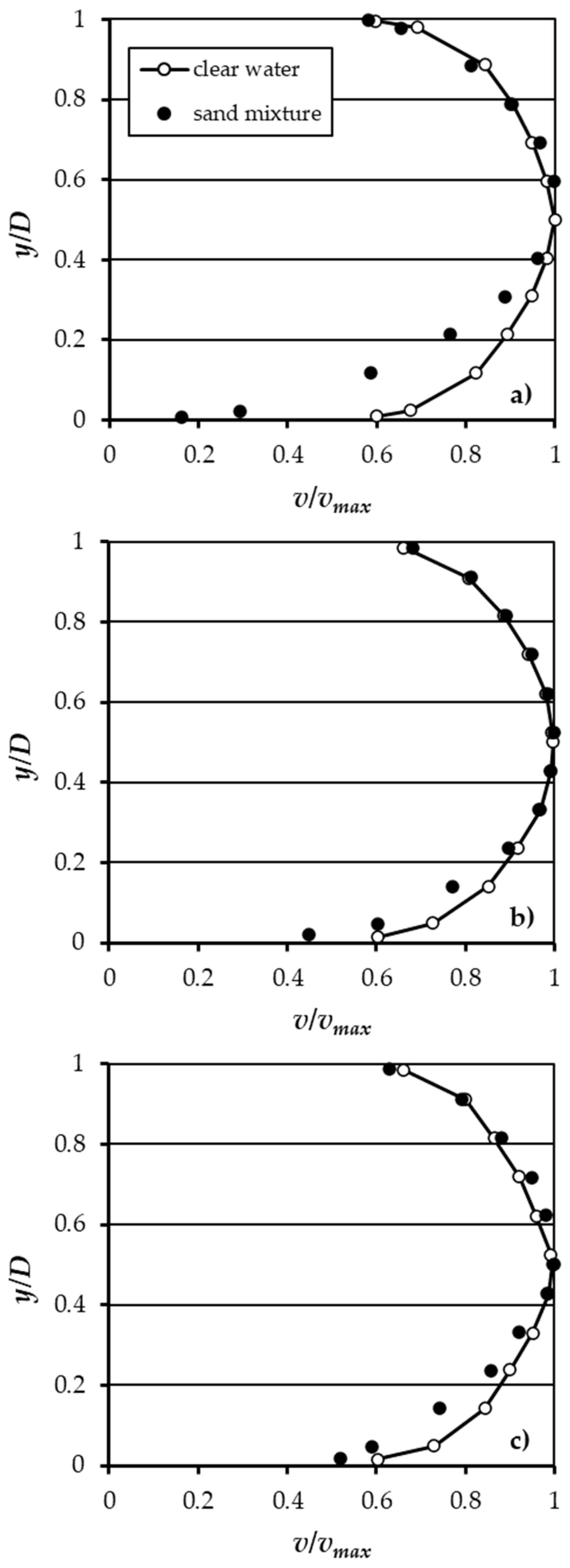
The velocity profile measurements plotted in Figure 2 in the plane for given hydraulic conditions (clear water and sand concentration of 0.054) and the three investigated sand mixtures (Dm = 0.88 mm, 0.41 mm and 0.30 mm) demonstrate that the effects of transported sediment particles are appreciable for the highest values of Dm (Figure 2a) and the differences in local flow velocity occur in the zone of the profile below the maximum velocity value (for y/D ≤ 0.5).
Considering that Equation (1) can be rewritten as:
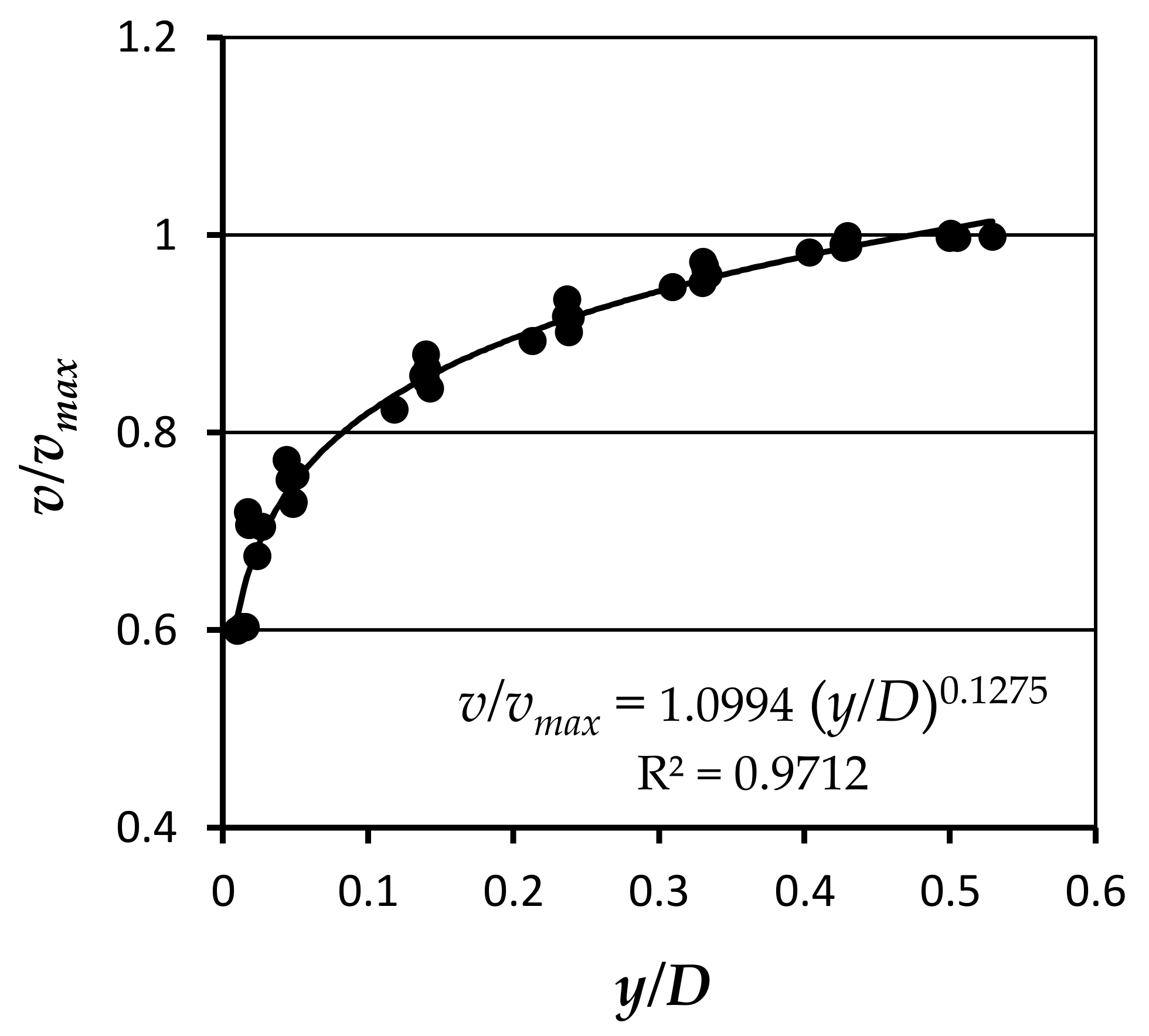
in which vmax is the maximum local velocity and is a coefficient. The measured pairs (v/vmax, y/D) allow to estimate the exponent δ of a power profile.
Figure 3, which shows the pairs (v/vmax, y/D) measured by Melisenda [5] for clear water, demonstrates that for the investigated flows δ is equal to 0.1275.
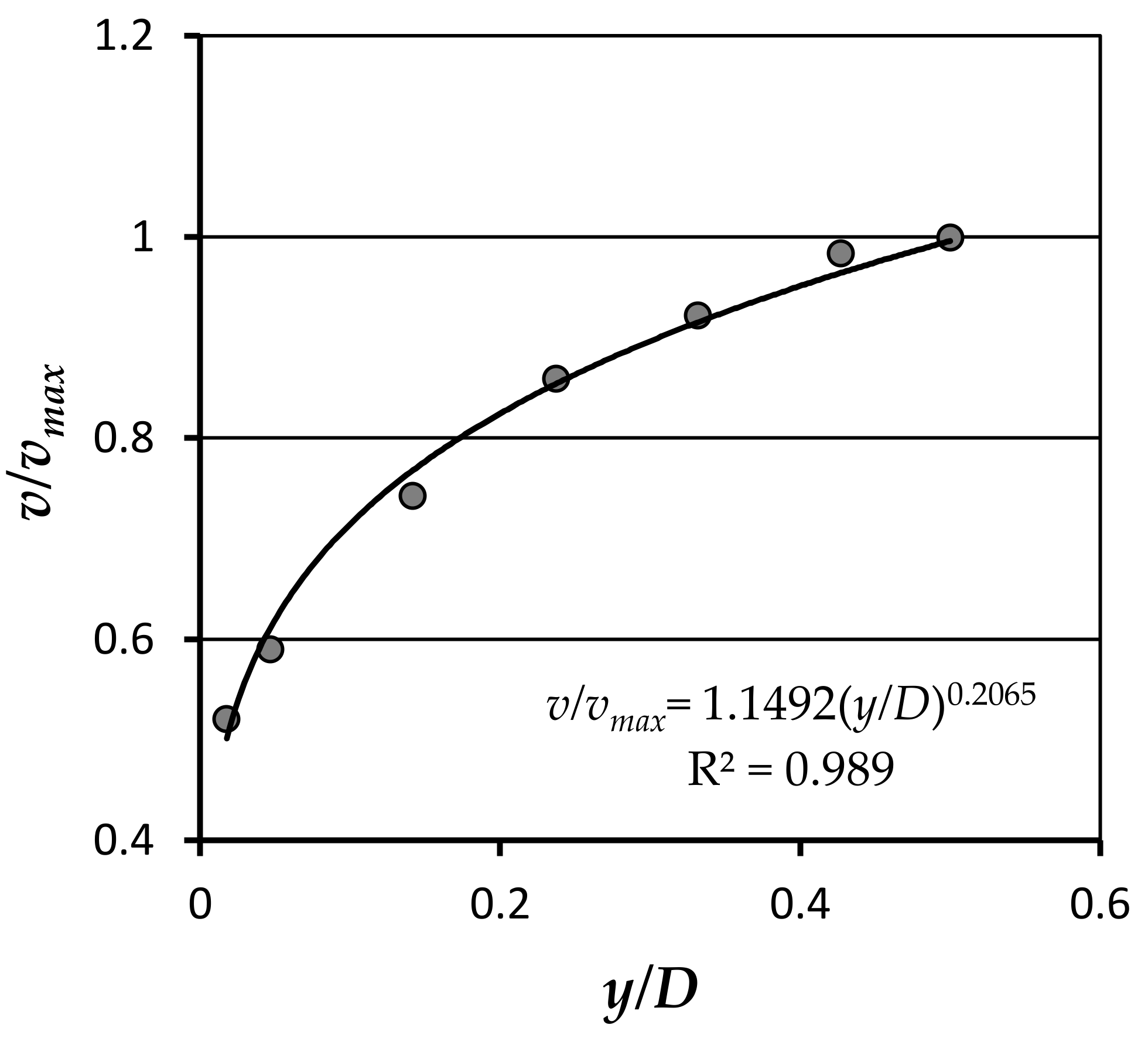
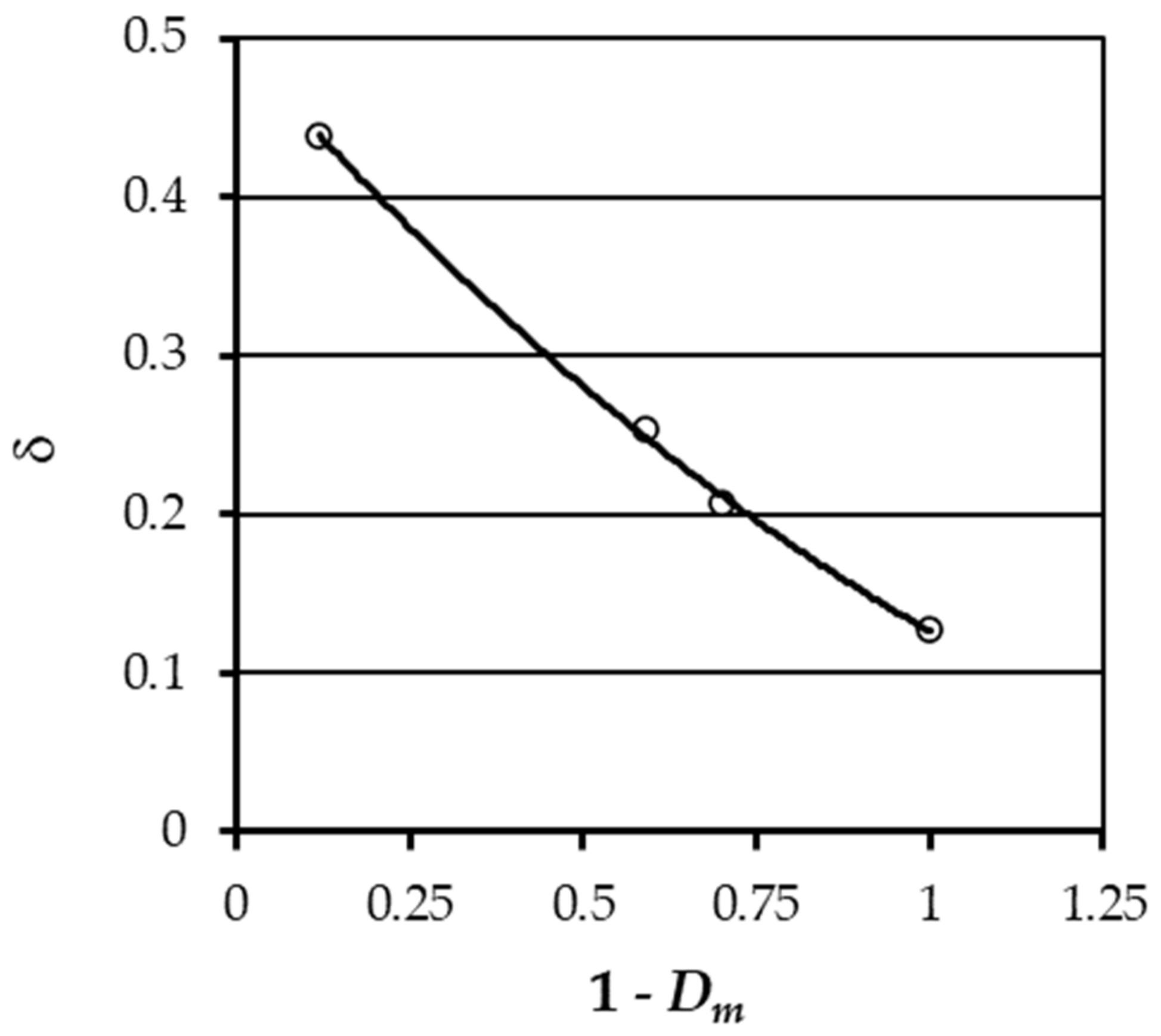
As an example, Figure 4 shows a velocity profile measured for the sand mixture, with Dm = 0.30 mm and a sand concentration of 0.054, and the power velocity profile having Equation (4) with δ = 0.2065. The analysis for the other two sand mixtures allowed to estimate δ = 0.2535 for Dm = 0.41 mm and δ = 0.4384 for Dm = 0.88 mm.
For the sand mixtures, the δ values, corresponding to a concentration of 0.054, were related to the particle size by the following relationship (Figure 5):
in which the median particle diameter Dm is expressed as mm. Equation (5) gives δ = 0.1275 for Dm = 0 (clear flow).
The mean flow velocity V along a diameter of the cross-section pipe is obtained integrating the velocity profile:
From Equation (6) the following equation is deduced:
and rearranging Equation (7) the following expression of the mean flow velocity is obtained:
From Equation (7) the following estimate, Гv, of the Г function is obtained:
Equation (9) allows to obtain Гv values corresponding to the measured head loss per unit length and the mean flow velocity (V = 4 Q/π D2) for a pipe flow having a discharge Q.
3.2. Flow Resistance
Taking into account that and , from Equation (3), the following equation is obtained [7]:
in which Гf is the estimate of the Г function obtained by the flow resistance equation. Equation (10) can be rewritten as follows:
Using Equation (11) and Equation (9) the following ratio is calculated:
For clear flow conditions, the Гv values calculated by Equation (9) were related to the head loss per unit length J according to the following relationship:
in which is a dimensionless group, named pipe flow Froude number, and a, b and c are three coefficients to be estimated by measurements. Equation (13) is similar to the relationship deduced for the open channel flows [15,16,17] in which the head loss per unit length and F are replaced with the channel slope and the Froude number , in which h is the channel flow depth, respectively.
For calculating Гv by Equation (9) the coefficient δ was set equal to 0.127 for the clear flow conditions investigated by Melisenda [5] and was calculated by Equation (2) with δo = 1.55 for the data by Butera et al. [9]. Using the available data base and least squares method, the coefficients a = 0.402, b =1.201 and c = 0.637 were estimated.
For testing the accuracy of the proposed approach for the clear flow condition, the measured values of the Darcy-Weisbach friction factor were compared with those calculated by Equation (3) with Гf estimated by Equations (12) and (13). Figure 6 shows a good agreement between the measured, fm, and the calculated, fc, Darcy-Weisbach friction factor values. The agreement is characterized by estimate errors E = (fc − fm)/fm, which are always less than or equal to ±10% and are less than or equal to ±5% for 91.4% of the cases.
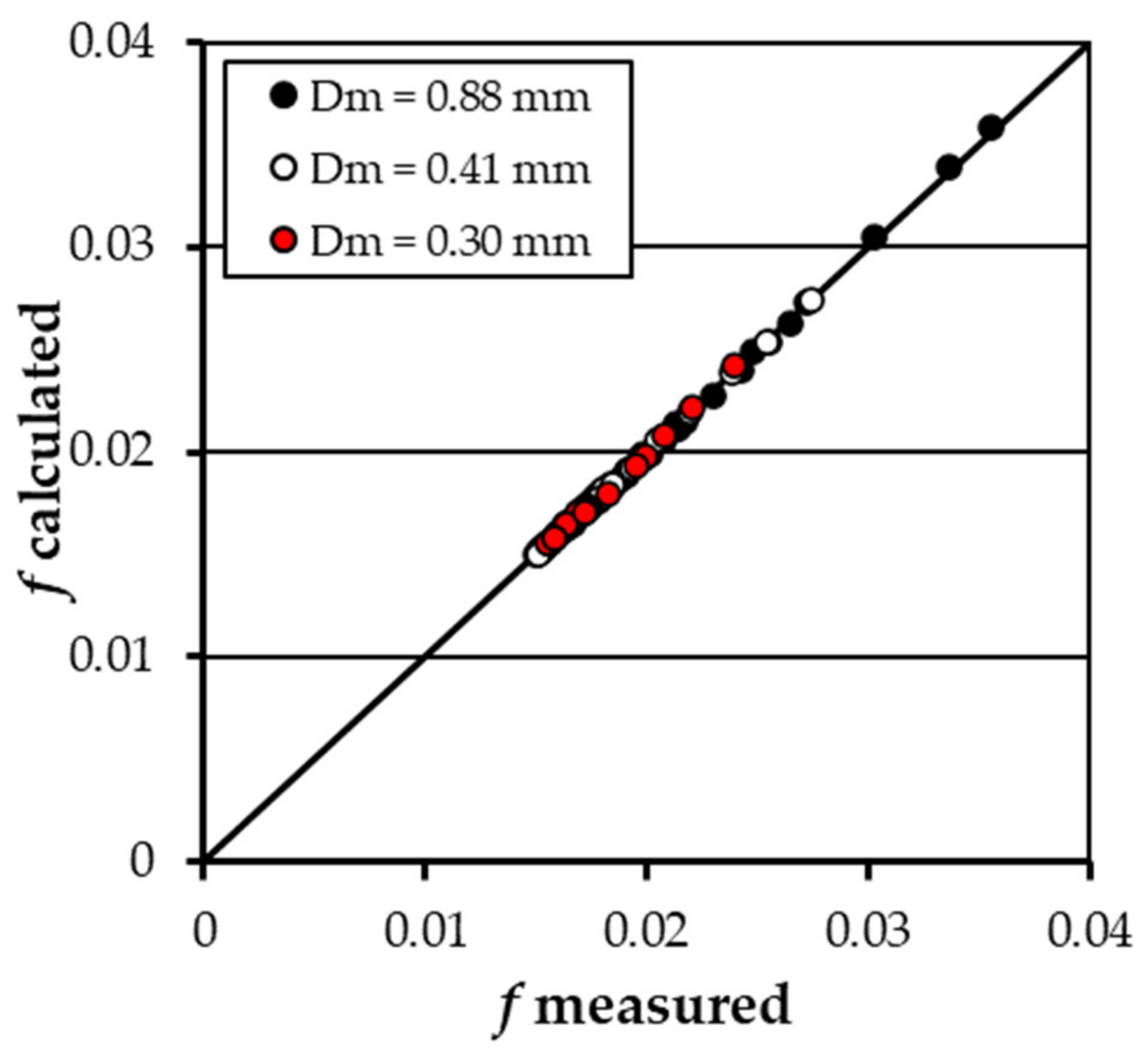
Using the available database of measurements carried out by sediment-laden flows having different concentration and a quasi-uniform sediment size characterized by three different values of the mean diameter Dm (0.88 mm, 0.41 mm and 0.30 mm) [5]; the values of the three coefficients a, b and c of Equation (13) were estimated (Table 1).
The accuracy of the proposed approach for the sediment-laden flow condition was tested comparing the measured values of the Darcy-Weisbach friction factor with those calculated by Equation (3) with Γf estimated by Equations (12) and (13) whose coefficients are listed in Table 1.
Figure 7 shows the good agreement between the measured, fm, and the calculated, fc, Darcy-Weisbach friction factor values which is characterized by estimate errors E = (fc − fm)/fm, which are always less than or equal to ±1.5% and are less than or equal to ±0.5% for 57.7% of the cases.
4. Discussion
4.1. Flow Velocity Profiles
For the investigated clear flows, characterized by 228,602 ≤ Re ≤ 238,574, the value δ = 0.127 estimated by velocity profiles (Figure 3) is very close to the value 0.121–0.122 which is calculated by Equation (2) with δo = 1.5 in the experimental Re range. According to Butera et al. [9], using δo = 1.55 and the experimental range 228,602 ≤ Re ≤ 238,574, δ varies from 0.125 to 0.126.
Equation (5) holds for the investigated sand mixtures characterized by known Dm values and a common sand concentration of 0.054. The δ values estimated by the measured velocity profiles and Equation (5) pointed out that δ increases with the sediment size. In other words, for a given discharge, the velocity profile for a flow with suspended sediments is characterized by velocity values less than those corresponding to the clear flow. Therefore, the experimental results suggest that the local flow velocity in a sediment-laden pipe flow is affected by sediment size and decreases in comparison with a clear-water flow having same hydraulic conditions. The differences between local velocity in a sediment-laden and a clear flow decrease with the mean sediment size Dm and are represented by the exponent δ of the velocity profile (δ = 0.127 for a clear flow and δ = 0.4384 for a sediment-laden flow with Dm = 0.88 mm).
4.2. Flow Resistance
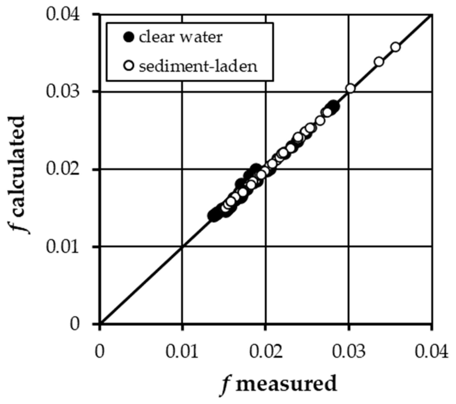
The developed analysis, which stated the independence of Гv on sediment concentration (see Equation (13)), confirmed in agreement with Di Stefano et al. [14] that for large-size mixtures (Dm > 0.2 mm) the effect of mean suspended sediment concentration can be neglected to estimate with accuracy the Darcy-Weisbach friction factor.
Figure 8, in which the f values are compared for clear water and sediment-laden flows, put into evidence that clear water flows are characterized by f values always less than 0.03 and, in comparison with Figure 7, that the effects of transported sediment particles (f > 0.03) are appreciable for the highest value of Dm (0.81 mm). This investigation allowed to establish how the sand suspended load determines a growth of flow resistance as compared to a clear-water flow in the same hydraulic conditions. The experimental results suggest that flow resistance in sediment-laden pipe flows increases for the highest values of the sediment size while, for the smallest values of Dm, the friction factor f is comparable with that of a clear flow having the same hydraulic conditions.
The experimental results allow to conclude that suspended load does not reduce the friction factor and this circumstance indirectly demonstrates that the sediment load does not damp flow turbulence. In any case, the proposed theoretical approach (Equations (3), (12) and (13)) allows an accurate estimate of pipe flow resistance for flows with a sediment-load constituted by sand-size particles.
5. Conclusions
In the past, a very limited number of studies were developed on friction factor in pipe sediment-laden flows and this topic is widely open to scientific debate. Flow resistance law was generally deduced by a theoretical approach when the velocity profile is known as for some cross-section shapes and defined boundary conditions.
In this paper, a theoretical approach, based on the integration of a power velocity distribution, deduced for both pipe and open channel flow was tested for the estimate of the Darcy-Weisbach friction factor for sediment-laden flow in pipes.
The analysis was developed by the following steps: (i) for the sediment-laden flows, the velocity profiles measured by Melisenda [5] were used to estimate the exponent d of the velocity profiles for the three investigated mixtures; (ii) a relationship between δ and the diameter Dm of the suspended sand was obtained; (iii) a relationship for estimating the coefficient Гv, obtained by the power-velocity profile (Equation (9)), and that Гf of the flow resistance law (Equation (11)) was theoretically deduced; (iv) the relationship between the coefficient Гv, the head loss per unit length and the pipe flow Froude number was obtained, and the procedure (Equations (3), (12) and (13)) to estimate the Darcy-Weisbach friction factor is tested by the available measurements.
The analysis allowed to state that the differences between local velocity in a sediment-laden and a clear flow decrease with the mean sediment size Dm and these differences are represented by the exponent δ of the velocity profile. The proposed approach to estimate the Darcy-Weisbach friction factor resulted accurate both for clear water and sediment-laden flow conditions using appropriate values of the coefficients a, b and c of Equation (13). For large-size mixtures (Dm > 0.2 mm) the Darcy-Weisbach friction factor can be accurately estimated neglecting the effect of mean concentration of suspended sediments. The flow resistance in sediment-laden pipe flows increased for the highest values of the sediment size and suspended load did not reduce the friction factor and, as a consequence, was not able to damp flow turbulence.
Further investigations should be carried out to test the influence of sediment size and concentration on pipe flow resistance and to relate the parameters of the local velocity distribution with the flow resistance equation.
Author Contributions
Both Authors contributed to outline the investigation, analyze the data, discuss the results, write the manuscript and approve it for publication. All authors have read and agreed to the published version of the manuscript.
Funding
This research received no external funding.
Institutional Review Board Statement
Not applicable.
Informed Consent Statement
Not applicable.
Data Availability Statement
The data presented in this study are available on request from the corresponding author.
Conflicts of Interest
The authors declare no conflict of interest.
References
- Kim, C.; Lee, M.; Han, C. Hydraulic transport of sand-water mixtures in pipelines. Part I. Experiment. J. Mech. Sci. Technol. 2008, 22, 2534–2541. [Google Scholar] [CrossRef]
- Leporini, M.; Marchetti, B.; Corvaro, F.; di Giovine, G.; Polonara, F.; Terenzi, A. Sand transport in multiphase flow mixtures in a horizontal pipeline: An experimental investigation. Petroleum 2019, 5, 161–170. [Google Scholar] [CrossRef]
- Garde, R.J. Sediment Transport through Pipes. Master’s Thesis, Colorado Agricultural and Mechanical College, Fort Collins, CO, USA, 1956. [Google Scholar]
- Swamee, P.K. Design of sediment-transporting pipeline. J. Hydraul. Eng. ASCE 1995, 121, 72–76. [Google Scholar] [CrossRef]
- Melisenda, I. Ricerca Sperimentale sul Trasporto Solido Nelle Correnti in Pressione; Istituto di Idraulica della Università di Palermo: Sicily, Italy, 1963. (In Italian) [Google Scholar]
- Craven, J.P. The transportation of sand in pipes I. Full pipe flow. In Proceedings of the Fifth Hydraulic Conference; Bulletin 34; State University of Iowa: Iowa City, IA, USA, 1953; Available online: https://ir.uiowa.edu/uisie/34/ (accessed on 28 July 2021).
- Ferro, V. Applying hypothesis of self-similarity for flow-resistance law of small-diameter plastic pipes. J. Irrig. Drain. Eng. ASCE 1997, 123, 175–179. [Google Scholar] [CrossRef]
- Barenblatt, G.I. Dimensional Analysis; Gordon &Breach, Science Publishers Inc.: New York, NY, USA, 1987. [Google Scholar]
- Butera, L.; Ridolfi, L.; Sordo, S. On the hypothesis of self-similarity for the velocity distribution in turbulent flows. Excerpta Ital. Contrib. Field Hydraul. Eng. 1993, 8, 63–94. [Google Scholar]
- Castaing, B.; Gagne, Y.; Hopfinger, E.J. Velocity probability density functions of high Reynolds number turbulence. Physica D 1990, 46, 177–200. [Google Scholar] [CrossRef]
- Barenblatt, G.I. On the scaling laws (incomplete self-similarity with respect to Reynolds numbers) for the developed turbulent flows in tubes. C. R. Acad. Sci. 1991, 313, 307–312. [Google Scholar]
- Nikuradse, J. Gesetzmassigkeiten der turbulenten Stromug in glatten Rohren. Ver Deutsch. Ing. Forschungsheft. 1932, 356, 1–36. [Google Scholar]
- Schlichting, H.; Karlsruhe, G. Grenschicht-Theorie; Springer: Heidelberg, Germay, 1968. [Google Scholar]
- Di Stefano, C.; Nicosia, A.; Palmeri, V.; Pampalone, V.; Ferro, V. Flow resistance law under suspended sediment laden conditions. Flow Meas. Instr. 2020, 74, 101771. [Google Scholar] [CrossRef]
- Ferro, V. New flow resistance law for steep mountain streams based on velocity profile. J. Irrig. Drain. Eng. ASCE 2017, 143, 1–6. [Google Scholar] [CrossRef]
- Ferro, V.; Porto, P. Applying hypothesis of self-similarity for flow resistance law in Calabrian gravel-bed rivers. J. Hydraul. Eng. ASCE 2018, 140, 1–11. [Google Scholar] [CrossRef]
- Carollo, F.G.; Ferro, V. Experimental study of boulder concentration effect on flow resistance in gravel bed channels. CATENA 2021, 205, 105458. [Google Scholar] [CrossRef]
Figure 1.
Scheme of the experimental layout used by Melisenda [5] (a) and view of the initial and final reaches of the experimental pipe (b) (modified from [5]).


Figure 2.
Velocity profile measurements for given hydraulic conditions (clear water and sand concentration of 0.054) and the three investigated sand mixtures (Dm = 0.88 mm (a), 0.41 mm (b) and 0.30 mm (c)).
Figure 2.
Velocity profile measurements for given hydraulic conditions (clear water and sand concentration of 0.054) and the three investigated sand mixtures (Dm = 0.88 mm (a), 0.41 mm (b) and 0.30 mm (c)).

Figure 3.
Velocity profile measured by Melisenda [5] for clear water.
Figure 3.
Velocity profile measured by Melisenda [5] for clear water.

Figure 4.
Velocity profile measured for the sand mixture, with Dm = 0.30 mm and a sand concentration of 0.054, and the power velocity profile having Equation (4) with δ = 0.2065.
Figure 4.
Velocity profile measured for the sand mixture, with Dm = 0.30 mm and a sand concentration of 0.054, and the power velocity profile having Equation (4) with δ = 0.2065.

Figure 5.
Relationship between the δ values, corresponding to a concentration of 0.054, and the particle size Dm, for sand mixtures.
Figure 5.
Relationship between the δ values, corresponding to a concentration of 0.054, and the particle size Dm, for sand mixtures.

Figure 6.
Comparison between the measured Darcy-Weisbach friction factor values, fm, and those calculated, fc, by Equation (3) with Гf estimated by Equations (12) and (13) with the coefficients a = 0.402, b =1.201 and c = 0.637.
Figure 6.
Comparison between the measured Darcy-Weisbach friction factor values, fm, and those calculated, fc, by Equation (3) with Гf estimated by Equations (12) and (13) with the coefficients a = 0.402, b =1.201 and c = 0.637.

Figure 7.
Comparison between the measured Darcy-Weisbach friction factor values, fm, and those calculated, fc, by Equation (3) with Γf estimated by Equations (12) and (13) with the coefficients listed in Table 1.
Figure 7.
Comparison between the measured Darcy-Weisbach friction factor values, fm, and those calculated, fc, by Equation (3) with Γf estimated by Equations (12) and (13) with the coefficients listed in Table 1.

Figure 8.
Comparison between the f values for clear water and sediment-laden flows.


Table 1.
Values of coefficients of Equation (13).
| Flow Condition | a | b | c |
|---|---|---|---|
| Clear flow | 0.402 | 1.201 | 0.637 |
| Sediment-laden flow Dm = 0.88 mm | 0.032 | 1.006 | 0.724 |
| Sediment-laden flow Dm = 0.41 mm | 0.199 | 0.982 | 0.617 |
| Sediment-laden flow Dm = 0.30 mm | 0.227 | 1.104 | 0.660 |
Publisher’s Note: MDPI stays neutral with regard to jurisdictional claims in published maps and institutional affiliations. |
© 2021 by the authors. Licensee MDPI, Basel, Switzerland. This article is an open access article distributed under the terms and conditions of the Creative Commons Attribution (CC BY) license (https://creativecommons.org/licenses/by/4.0/).
Share and Cite
MDPI and ACS Style
Ferro, V.; Nicosia, A. Evaluating the Effects of Sediment Transport on Pipe Flow Resistance. Water 2021, 13, 2091. https://doi.org/10.3390/w13152091
AMA Style
Ferro V, Nicosia A. Evaluating the Effects of Sediment Transport on Pipe Flow Resistance. Water. 2021; 13(15):2091. https://doi.org/10.3390/w13152091
Chicago/Turabian StyleFerro, Vito, and Alessio Nicosia. 2021. "Evaluating the Effects of Sediment Transport on Pipe Flow Resistance" Water 13, no. 15: 2091. https://doi.org/10.3390/w13152091
Note that from the first issue of 2016, this journal uses article numbers instead of page numbers. See further details here.