Assessing the Impact of Wave–Current Interactions on Storm Surges and Waves during Cold Air Outbreaks in the Northern East China Sea

Abstract

Storm surges and disastrous waves induced by cold air outbreaks, a type of severe weather system, often impact the coastal economic development. Using the Climate Forecast System Reanalysis wind product and the Coupled Ocean–Atmosphere–Wave–Sediment Transport model, we developed a coupled numerical model and applied it to examine the interaction between surface gravity waves and ocean currents during cold air outbreaks in two case studies in the northern East China Sea. The results revealed that wave–current interactions improved the simulation accuracy, especially the water level, as verified by tidal station measurements. We conducted sensitivity experiments to explore the spatiotemporal variation of the impact of wave–current interactions on storm surges and waves in the northern East China Sea, away from the coastline. The wave-induced surge (up to 0.4 m) and the wave-induced current (up to 0.5 m/s) were found to be related to the difference between wave direction and current direction. The significant wave height difference (up to 0.5 m) was sensitive to the storm surge nearshore and sensitive to the current field offshore, while the mean wave direction change (up to 40°) was more sensitive to the current field than to the storm surge. Additionally, the wave–current interaction regulated the momentum balance and wave action balance, respectively. By comparison, the momentum residuals of pressure gradient, Coriolis force, Coriolis–Stokes force, and bottom stress, which were pronounced in different areas, were modulated more significantly by the wave effect than other terms. The dominant mechanisms of wave–current interactions on waves included the current-induced modification of energy generation caused by wind input, the current-induced modification of energy dissipation caused by whitecapping, and the current-induced wave advection.

1. Introduction

Storm surges and huge waves induced by cold air outbreaks (CAOs, also known as cold waves) adversely affect the economic development of coastal cities [1,2,3]. Researchers have simulated the marine dynamic environment during CAOs using numerical models and hindcasted the water level, currents, and waves separately [4,5,6]. The research on a single dynamic process, however, is not sufficient to describe the actual marine dynamic environment [7,8]. This insufficient understanding of the wave–current interaction mechanisms that modulate marine dynamic environmental factors is one of the key bottlenecks restricting the accurate forecasting and risk assessment of disastrous marine dynamic environments induced by CAOs [9]. Therefore, it is necessary and urgent to study wave–current interactions during CAOs [10].

Significant momentum and energy exchanges occur when wind-driven waves and currents meet [11]. The two main representations of wave–current interaction are the radiation stress mechanism and the vortex force mechanism. Progressive-scale analysis and numerical simulation have demonstrated that the vortex force mechanism is more accurate than the radiation stress mechanism [12,13,14]. Wave–current interaction mechanisms also include wind effects, bottom friction, wave breaking, and other forcing and dissipation mechanisms. The relative wind effect is an important wave–current interaction mechanism and is able to generate 20–40% current modulation for wave height [15]. In shallow water, the wave direction can be modulated up to 70° by currents [16]. Waves can increase the sea surface roughness and enhance the wind stress, which in turn modulate the current field [17]. In addition, the bottom friction can also be changed by waves, while breaking waves, nonbreaking waves, and their induced Coriolis–Stokes force and Langmuir circulation all influence the dynamics of the upper-ocean layer [18,19,20,21]. Researchers have established a few wave–current coupled models to simulate the ocean dynamic processes and have actively explored the parameterization schemes of wave–current interactions [22,23,24,25]. As a result, the development of numerical simulations is deepening our understanding of the physical mechanisms of wave–current interactions [26,27,28,29].

Studies on wave–current interaction have focused mainly on tropical cyclones, while less attention has been paid to other weather systems [30]. Strong winds in coastal areas can cause dramatic changes in water level and currents, which influence wave height and direction, thereby increasing hazardous conditions [31]. Wave parameters in the outer region of the typhoon are more sensitive to the current but less sensitive to the water elevation than those in the inner region of the typhoon [32]. Currents generated by tropical cyclones can increase a wave group’s translation speed, reduce wave height, and expand the wave direction distribution [33]. Importantly, the dominant mechanisms of wave–current interactions differ on either side of the storm track. As a result of waves, the momentum flux input from the wind field to the surface current is significantly reduced and varies by as much as ~25% with the forward speed and intensity of the tropical cyclone [34,35]. The effect of waves on water level is greater in shallow coastal waters while the occurrence times of wave set-up and storm surge vary [36,37,38]. The effect of waves on currents reaches its maximum, about 40% more than the Ekman current, during the rapid development stage of storms [39].

In fact, CAOs occur more frequently and are more destructive than tropical cyclones at high latitudes [40,41]. The Bohai Sea and the northern Yellow Sea, also known as the northern East China Sea (NECS, Figure 1), frequently experience CAOs [42]. Because of the asymmetry of the wind field on both sides of tropical cyclone tracks, wave–current interactions during tropical cyclones depend heavily on tracks and regions. The CAOs whose tracks are visible only over Eurasia are characterized mainly by persistent strong winds in the NECS. Although storm surges driven by CAOs are smaller than those driven by tropical cyclones, the duration of storm surges is longer, the affected area is larger, and the variation range of the flow field is also larger. Measured data have shown that the wind–wave growth relationships generated by CAOs are very obvious [43]. Therefore, the wave–current interaction mechanism during CAOs is assumed to be different from the mechanism during tropical cyclones. This study assessed the impact of wave–current interactions on dynamic marine environmental factors, such as sea level, currents, and waves, during CAOs. The coupled model and its set-up are described in Section 2. The simulation results with and without consideration of wave–current interactions are presented in Section 3. In Section 4, the contributions of wave–current interactions are evaluated, and their physical mechanisms are discussed. The summary and conclusions are provided in Section 5.

2. Coupled Model and Numerical Experiments

2.1. Model Description

The Coupled Ocean–Atmosphere–Wave–Sediment Transport (COAWST) modeling system was developed by Warner et al. [44] from the U.S. Geological Survey, Coastal and Marine Science Center, Woods Hole, United States. This coupling system has been widely used to study near-shore physical processes on a regional scale [13,45,46]. To explore the impacts of wave–current interactions induced by CAOs, in this study, we used COAWST (version 3.2) to establish a three-dimensional numerical model of wave–current coupling.

COAWST is composed of ocean, atmosphere, wave, and sediment transport modules, as well as couplers for exchanging data. The ocean module of COAWST is the Regional Ocean Model System (ROMS) [47], and its wave module is Simulating WAves Nearshore (SWAN) [48]. The Model Coupling Toolkit (MCT) coupler is used for data exchange and transmission among the different modules in parallel computing. The ROMS provides data such as current field, terrain, and sea level for SWAN and SWAN provides data such as wave factors and wave energy dissipation for the ROMS. The two modules are two-way coupled.

2.1.1. Hydrodynamic Model

Under the assumption of vertical hydrostatics and the Boussinesq approximation, the primitive equations in the ROMS are free-surface, Reynolds-averaged, Navier–Stokes equations, which are solved using finite difference methods. In the horizontal Cartesian and vertical sigma coordinates, the momentum balance equations in the ROMS are as follows:

$$\underset{ACC}{\underbrace{\frac{\partial \left(H_{z}u\right)}{\partial t}}}+\underset{HA}{\underbrace{\frac{\partial \left(u{H}_{z}u\right)}{\partial x}+\frac{\partial \left(v{H}_{z}u\right)}{\partial y}}}+\underset{VA}{\underbrace{\frac{\partial \left(\omega H_{z}u\right)}{\partial s}}}\underset{COR}{\underbrace{-f{H}_{z}v}}=\underset{PG}{\underbrace{-H_z\frac{\partial \varphi }{\partial x}}}\underset{VM}{\underbrace{-\frac{\partial }{\partial s}\left(\overline{u^{\prime }{w}^{\prime }}-\frac{\nu }{H_z}\frac{\partial u}{\partial s}\right)}}+\underset{BF}{\underbrace{H_z{F}_u}}+\underset{HM}{\underbrace{H_z{D}_u}},$$

(1)

$$\underset{ACC}{\underbrace{\frac{\partial \left(H_{z}v\right)}{\partial t}}}+\underset{HA}{\underbrace{\frac{\partial \left(u{H}_{z}v\right)}{\partial x}+\frac{\partial \left(v{H}_{z}v\right)}{\partial y}}}+\underset{VA}{\underbrace{\frac{\partial \left(\omega H_{z}v\right)}{\partial s}}}+\underset{COR}{\underbrace{f{H}_{z}u}}=\underset{PG}{\underbrace{-H_z\frac{\partial \varphi }{\partial y}}}\underset{VM}{\underbrace{-\frac{\partial }{\partial s}\left(\overline{v^{\prime }{w}^{\prime }}-\frac{\nu }{H_z}\frac{\partial v}{\partial s}\right)}}+\underset{BF}{\underbrace{H_z{F}_v}}+\underset{HM}{\underbrace{H_z{D}_v}},$$

(2)

$$\frac{\partial \varphi }{\partial s}=-\frac{H_z\rho g}{{\rho }_0}.$$

(3)

Based on the incompressible approximation, the continuity equation is:

$$\frac{\partial \left(H_{z}u\right)}{\partial x}+\frac{\partial \left(H_{z}v\right)}{\partial y}+\frac{\partial \left(H_z\omega \right)}{\partial s}=0,$$

(4)

where (u, v) represent the horizontal (x and y) components of the mean velocity (s); $\omega$ represents the vertical (s) component of the mean velocity; the vertical s coordinate is negative downward with s = 0 at mean sea level and s = −1 at the bottom; $H_z$ is the grid-cell thickness; f is the Coriolis parameter; g is the acceleration of gravity; $\rho$ and ${\rho }_0$ are the total and reference densities of seawater; $\nu$ is the molecular viscosity parameter; $\varphi$ represents the dynamic pressure; $F_u$ and $F_v$ represent the Reynolds stresses; $\overline{u^{\prime }{w}^{\prime }}$ and $\overline{v^{\prime }{w}^{\prime }}$ represent the body forces; $D_u$ and $D_v$ represent the horizontal mixing terms. As shown by Kumar et al. [13], the terms from left to right in Equations (1) and (2) are the local acceleration (ACC), the horizontal advection (HA), the vertical advection (VA), the Coriolis force (COR), the pressure gradient (PG), the vertical mixing (VM), the body force (BF), and the horizontal mixing (HM) terms. The Reynolds stresses can be parameterized as follows:

$$\overline{u^{\prime }{w}^{\prime }}=-\frac{K_M}{H_z}\frac{\partial u}{\partial s},$$

(5)

$$\overline{v^{\prime }{w}^{\prime }}=-\frac{K_M}{H_z}\frac{\partial v}{\partial s},$$

(6)

where is the eddy viscosity for momentum. The vertical boundary conditions for the Reynolds stresses are:

$$\frac{K_M}{H_z}\frac{\partial u}{\partial s}|\begin{array}{c}\\ s=0\end{array}={\tau }_s^x\left(x, y, t\right),$$

(7)

$$\frac{K_M}{H_z}\frac{\partial v}{\partial z}|\begin{array}{c}\\ s=0\end{array}={\tau }_s^y\left(x, y, t\right),$$

(8)

$$\frac{K_M}{H_z}\frac{\partial u}{\partial z}|\begin{array}{c}\\ s=-1\end{array}={\tau }_b^x\left(x, y, t\right),$$

(9)

$$\frac{K_M}{H_z}\frac{\partial v}{\partial z}|\begin{array}{c}\\ s=-1\end{array}={\tau }_b^y\left(x, y, t\right),$$

(10)

where $\left({\tau }_s^x, {\tau }_s^y\right)$ are the components of surface wind stress (Sstr), and $\left({\tau }_b^x, {\tau }_b^y\right)$ are the components of bottom stress (Bstr).

On the basis of the vortex–force coupling scheme, the momentum balance equations in COAWST are written as follows:

$$\begin{gathered} \underset{ACC}{\underbrace{\frac{\partial \left(H_{z}u\right)}{\partial t}}}+\underset{HA}{\underbrace{\frac{\partial u{H}_z\left(u+u^{St}\right)}{\partial x}+\frac{\partial u{H}_z\left(v+v^{St}\right)}{\partial y}}}+\underset{VA}{\underbrace{\frac{\partial u{H}_z\left(\omega +{\omega }_s^{St}\right)}{\partial s}}}\underset{COR}{\underbrace{-f{H}_{z}v}}\underset{StCOR}{\underbrace{-f{H}_z{v}^{St}}}=\underset{PG}{\underbrace{-H_z\frac{\partial \varphi }{\partial x}}}+ \\ \underset{HVF}{\underbrace{H_z{v}^{St}\left(\frac{\partial v}{\partial x}-\frac{\partial u}{\partial y}\right)}}\underset{VVF}{\underbrace{-{\omega }_s^{St}\frac{\partial u}{\partial s}}}\underset{VM}{\underbrace{-\frac{\partial }{\partial s}\left(\overline{u^{\prime }{w}^{\prime }}-\frac{\nu }{H_z}\frac{\partial u}{\partial s}\right)}}+\underset{BF}{\underbrace{H_z{F}_u}}+\underset{HM}{\underbrace{H_z{D}_u}}, \end{gathered}$$

(11)

$$\begin{gathered} \underset{ACC}{\underbrace{\frac{\partial \left(H_{z}v\right)}{\partial t}}}+\underset{HA}{\underbrace{\frac{\partial v{H}_z\left(u+u^{St}\right)}{\partial x}+\frac{\partial v{H}_z\left(v+v^{St}\right)}{\partial y}}}+\underset{VA}{\underbrace{\frac{\partial v{H}_z\left(\omega +{\omega }_s^{St}\right)}{\partial s}}}+\underset{COR}{\underbrace{f{H}_{z}u}}+\underset{StCOR}{\underbrace{f{H}_z{u}^{St}}}= \\ \underset{PG}{\underbrace{-H_z\frac{\partial \varphi }{\partial y}}}\underset{HVF}{\underbrace{-H_z{u}^{St}\left(\frac{\partial v}{\partial x}-\frac{\partial u}{\partial y}\right)}}\underset{VVF}{\underbrace{-{\omega }_s^{St}\frac{\partial v}{\partial s}}}\underset{VM}{\underbrace{-\frac{\partial }{\partial s}\left(\overline{v^{\prime }{w}^{\prime }}-\frac{\nu }{H_z}\frac{\partial v}{\partial s}\right)}}+\underset{BF}{\underbrace{H_z{F}_v}}+\underset{HM}{\underbrace{H_z{D}_v}}, \end{gathered}$$

(12)

where $\left(u^{St},v^{St},{\omega }^{St}\right)$ are the components of the Stokes drift velocity. Compared to Equations (1) and (2), the expressions of HA and VA have changed due to Stokes drift. The added term on the left side of Equations (11) and (12) is the Stokes–Coriolis force (StCOR), and the added terms on the right side are the horizontal vortex force (HVF) and the vertical vortex force (VVF).

2.1.2. Wave Model

As a third-generation wave model, SWAN is suitable for wave simulations in coastal regions. SWAN solves the transport equation for wave action density spectrum $N\left(x,y, t;\sigma ,\theta \right)$. In Cartesian coordinates, the action balance equations are as follows:

$$\frac{\partial N}{\partial t}+\frac{\partial c_{x}N}{\partial x}+\frac{\partial c_{y}N}{\partial y}+\frac{\partial c_{\sigma }N}{\partial \sigma }+\frac{\partial c_{\theta }N}{\partial \theta }=\frac{S_{tot}}{\sigma },$$

(13)

$$\left(c_x,c_y\right)=\overrightarrow{c_g}+\overrightarrow{U}=\frac{1}{2}\left[1+\frac{2|\overrightarrow{k}|d}{\sin h(2|\overrightarrow{k}|d)}\right]\frac{\sigma \overrightarrow{k}}{{|\overrightarrow{k}|}^2}+\overrightarrow{U},$$

(14)

$$c_{\sigma }=\frac{\partial \sigma }{\partial d}\left(\frac{\partial d}{\partial t}+\overrightarrow{U}·{\nabla }_{\overrightarrow{x}}d\right)-c_g\overrightarrow{k}·\frac{\partial \overrightarrow{U}}{\partial n},$$

(15)

$$c_{\theta }=-\frac{1}{k}\left(\frac{\partial \sigma }{\partial d}\frac{\partial d}{\partial m}+\overrightarrow{k}·\frac{\partial \overrightarrow{U}}{\partial m}\right),$$

(16)

where $c_x$, $c_y$, $c_{\sigma }$, and $c_{\theta },$ respectively, represent the propagation velocities of wave energy in spatial x- and y-space (PropXY) and in spectral $\sigma$-space (PropSigma) and in $\theta$-space (PropTheta); d is the water depth; $\overrightarrow{U}$; and (n, m) are the space coordinates parallel and perpendicular to the wave direction, $\theta$, respectively. $S_{tot}$ represents the wave energy generation and dissipation processes: energy generation due to wind input (GenWind), energy dissipation due to whitecapping (DisWcap), energy dissipation due to bottom friction (DisBot), energy dissipation due to surface breaking (DisSurf), and nonlinear wave–wave interactions. In coupled models, the energy transfer between waves and currents (TranCur) should be also considered.

2.2. Model Set-Up

Based on the COAWST modeling system, we developed a three-dimensional coupled model and set 16 vertical sigma levels for the ROMS. Coupling of the ROMS and SWAN was achieved using vortex force formalism [49]. The coupling time step was set to 10 min. The computational domains of the ROMS and SWAN covered a sea area larger than the NECS (30.0–41.0° N, 117–127° E), as shown in Figure 1, to consider the water movement throughout the entire East China Sea. The rectangular orthogonal grid, with a 1 arcmin grid size in zonal and meridional directions, was used in the ROMS and SWAN models. We obtained the bathymetry from the ETOPO-1 dataset (http://www.ngdc.noaa.gov/mgg/global/global.html, accessed on 30 July 2021) and set the minimum depth to 5 m. For the ROMS, the lateral boundaries were closed to the north and west. The initial conditions, open lateral boundary conditions, and sea surface temperature and salinity forcing conditions were provided by HYbrid Coordinate Ocean Model (HYCOM) data (http://hycom.org/data/glba0pt08, accessed on 30 July 2021). For SWAN, we performed the simulations in the nonstationary mode. Wave spectra were calculated in 36 isometric propagation directions and 35 logarithmic interval frequencies between 0.04 Hz and 1 Hz. A series of sensitivity experiments have been conducted to determine the parameterization schemes of ROMS and SWAN, e.g., bottom drag coefficient and whitecapping parameters. Given space limitation, this article does not cover the details of these parameterization schemes.

As the main driving forces, wind and pressure play key roles in the numerical simulation of ocean currents and waves. Researchers have compared wind data derived from satellite measurements, analysis, reanalysis, and WRF-modeled winds with in situ measurements to assess the best alternative to in situ measured wind data [50]. The reanalysis winds were proven to have relative superiority [51]. For typhoon winds, previous studies often blend the reanalysis winds into the parametric typhoon model to obtain good simulation results [52,53]. However, there is still no widely recognized atmospheric model of CAOs.

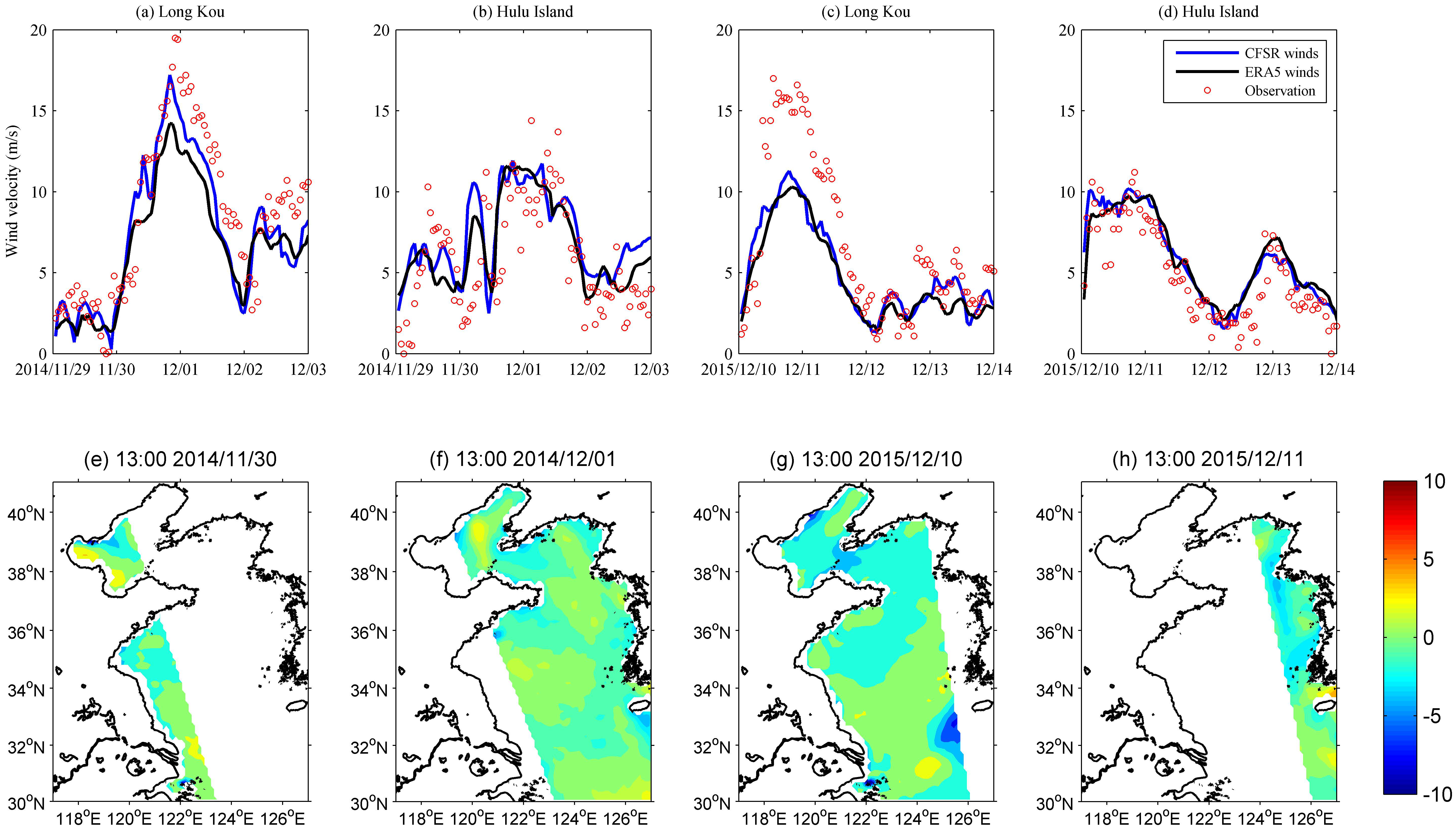
The general wind products mainly include the National Centre for Atmospheric Research (NCAR) products NCEP, NCEP2, CCMP and CFSR, and the European Centre for Medium-Range Weather Forecasts (ECMWF) product ERA5 and ERA40 reanalysis. Due to the low spatiotemporal resolutions and unsuitable temporal range, NECP, NECP2, CCMP and ERA40 are not appropriate to establish the surface wind forcing in this study. Hence, a comparison of the wind velocity from ERA5 and CFSR with observed winds from the available tidal stations (Long Kou and Hu Lu Dao) during the two events is presented in Figure 2a–d. At the nearshore stations, the two blended winds agree reasonably well with the observations on the variation trend, but this is not so when the wind speed is high. By comparison, the CFSR winds show higher correlations and lower root-mean-square errors than the ERA5 winds. Because of the lack of measured data, we also used the ASCAT scatterometer swath observations on MetOp-A to verify the accuracy of the CFSR wind product. The difference between CFSR wind speed and the ASCAT observed wind speed in the computational domain at validity time during the two events is shown in Figure 2e–h. It shows that the CFSR wind was consistent (differences less than 3 m/s) with the satellite observations in most areas when the wind was not strong (less than 6 on the Beaufort scale). Furthermore, the difference between CFSR wind and ASCAT product is greater in coastal areas than in center areas of the sea. Therefore, the surface forcing (i.e., wind field and surface pressure) for the ROMS and SWAN was derived from CFSR data (http://cfs.ncep.noaa.gov/cfsr/, accessed on 30 July 2021).

It is worth noting that because this study focused mainly on the interactions between waves and wind-driven currents, we did not consider the effects of astronomical tides, heat and moisture fluxes, and river discharge to avoid interference.

2.3. Experiments Design

Mo et al. [42] showed that different types of CAO-induced winds, known as generalized northwest (GNW) winds and generalized northeast (GNE) winds, induce different sea states. In this study, one representative event of each wind type was considered. The first event occurred in late November and early December 2014 and the second event was in mid-December 2015. For each CAO event, we performed five numerical experiments (

Table 1. Designs of the numerical experiments.

Experiment ID	Model Name	Water Level	Current	Wave
Exp1	ROMS	Y	Y	N
Exp2	SWAN	N	N	Y
Exp3	ROMS + SWAN	Y	N	Y
Exp4	ROMS + SWAN	N	Y	Y
Exp5	ROMS + SWAN	Y	Y	Y

), including a circulation-only experiment (Exp1), a wave-only experiment (Exp2), a wave–water level coupled experiment (Exp3), a wave–current coupled experiment (Exp4), and a wave–circulation fully coupled experiment (Exp5).

We collected in situ water level measured data from four tidal stations and wave height measured data from five buoys (Figure 1). The storm surge represents the de-tiding water level that is calculated by subtracting astronomical tide, obtained by harmonic analysis of hourly water level data for 366 days, from the total observed water level. For precision, 68 harmonics have been used.

3. Model Validation

3.1. CAO-Induced GNW Wind

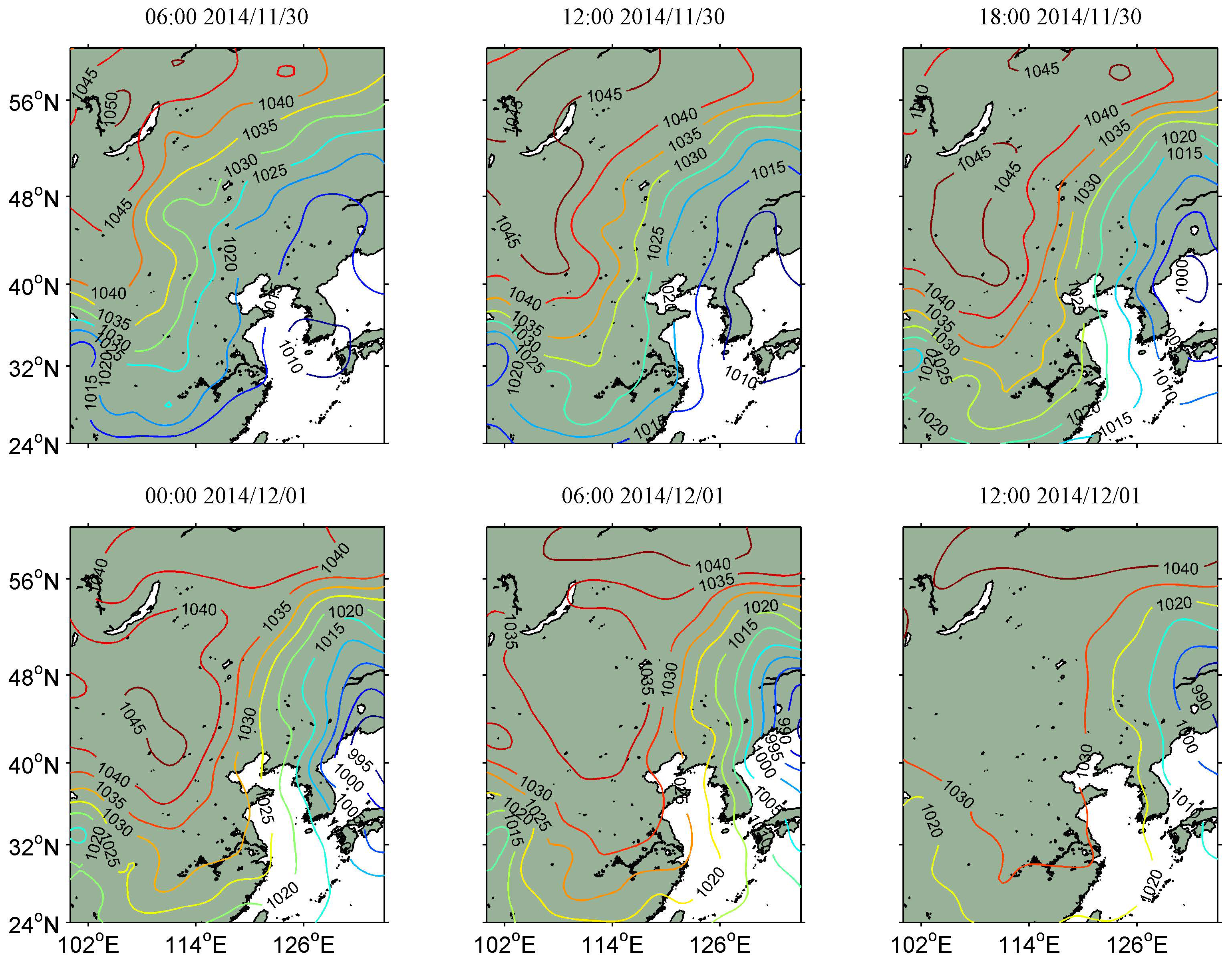
Based on the CFSR data, the evolution of mean sea level pressure distribution from 30 November to 1 December 2014 is shown in Figure 3. The cold air messes assembled in eastern Siberia and formed the surface high pressure at 1051 hPa early on November 30 (UTC, the same hereafter). As the cold high pressure moved southeastward, a low-pressure system appeared in the Japan Sea. The cold air, led by the NE–SW cold front, brought strong and homogeneous GNW wind exceeding 6 on the Beaufort scale to the NECS. As time passed, the intensity of the CAO gradually increased, resulting in an instantaneous maximum wind speed exceeding 9 on the Beaufort scale. On December 2, the CAO intensity gradually diminished, and the GNW wind decreased.

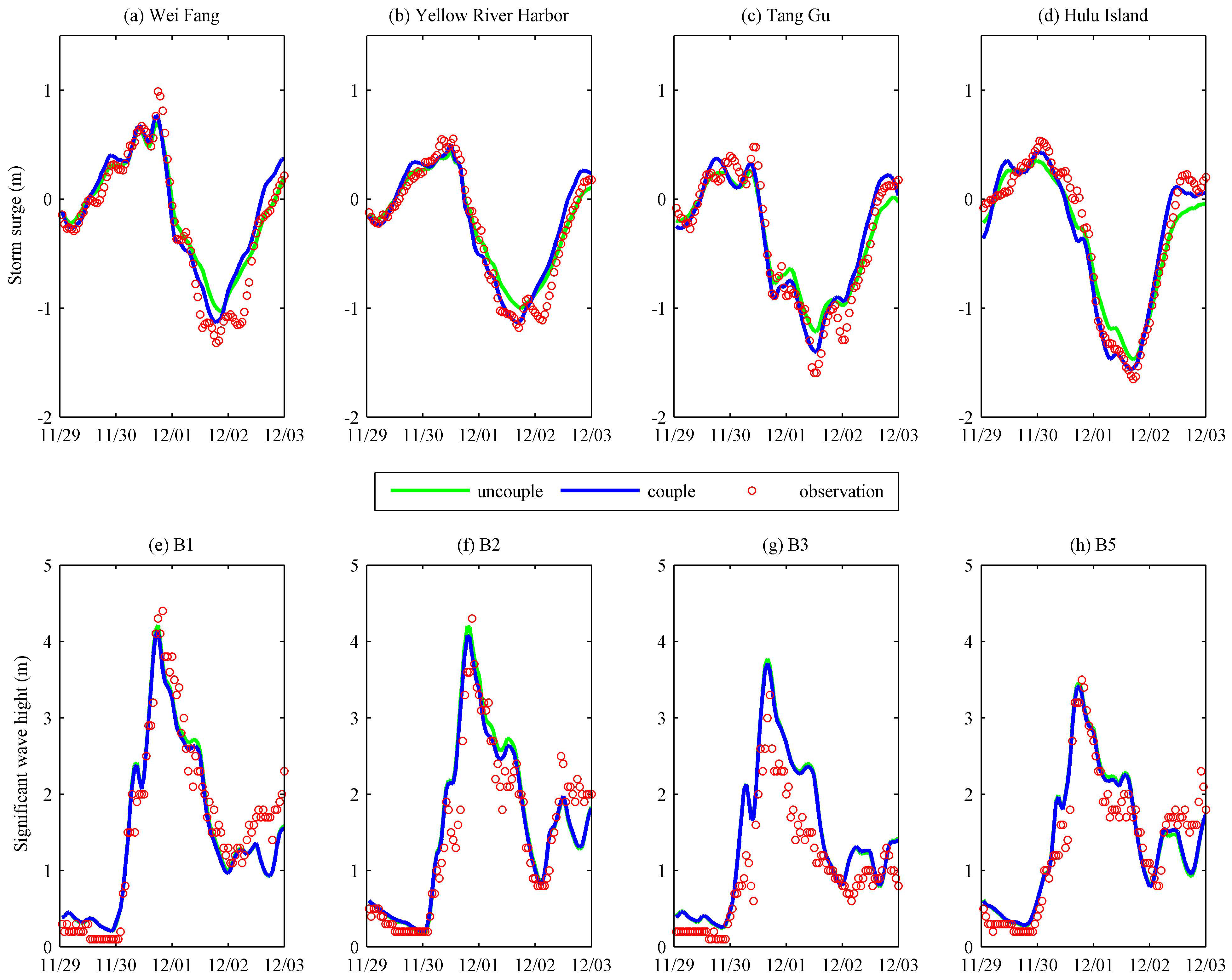
As shown in Figure 4, we compared the model-simulated storm surges and significant wave heights (SWHs) directly with observed data at the four coastal tidal stations and the four buoys available in the model domain. To quantitatively evaluate the accuracy of the uncoupled and coupled simulations, three error statistics were selected: the maxima relative error (MRE), root-mean-square error (RMSE), and correlation coefficient (CC). The calculation formulas are as follows:

$$\mathrm{MRE}=\frac{\left|P_{imax}-O_{imax}\right|}{O_{imax}}\times 100\%,$$

(17)

$$\mathrm{RMSE}=\sqrt{\frac{1}{n}{{\displaystyle \sum }}_{i=1}^n{\left(P_i-O_i\right)}^2},$$

(18)

$$\mathrm{CC}=\frac{{{\displaystyle \sum }}_{i=1}^n\left(P_i-\overline{P}\right)\left(O_i-\overline{O}\right)}{\sqrt{\left({{\displaystyle \sum }}_{i=1}^n{\left(P_i-\overline{P}\right)}^2\right)\left({{\displaystyle \sum }}_{i=1}^n{\left(O_i-\overline{O}\right)}^2\right)}},$$

(19)

where P_i and O_i represent the i-th simulated value and observed value in the time series, n is the total number of samples, and the overbar marks the arithmetic mean. As shown in

Table 2. Statistical comparisons between observations and simulations (Exp1, Exp2, and Exp5) during the CAO-induced GNW wind.

Tidal Stations and Buoys	Latitude (° N)	Longitude (° E)	MRE		RMSE (m)		CC
			Exp1 or Exp2	Exp5	Exp1 or Exp2	Exp5	Exp1 or Exp2	Exp5
Wei Fang	37.23	119.18	22%	15%	0.18	0.20	0.98	0.96
Yellow River Harbor	38.10	118.97	15%	4.2%	0.12	0.14	0.99	0.97
Tang Gu	38.98	117.78	24%	12%	0.16	0.15	0.98	0.97
Hulu Island	40.70	120.98	11%	5.3%	0.16	0.16	0.98	0.97
B1	38.02	119.51	4.3%	6.3%	0.34	0.34	0.96	0.96
B2	38.33	121.09	2.5%	5.8%	0.41	0.38	0.94	0.94
B3	38.53	119.00	14%	12%	0.52	0.50	0.95	0.95
B5	39.01	120.04	1.3%	3.0%	0.33	0.31	0.93	0.93

MRE represents the relative error of the extreme values in the time series of simulation; RMSE represents the root-mean-square error between the time series of observation and the time series of simulation; CC represents the correlation coefficient between the time series of observation and the time series of simulation.

, the coherence between the model simulations (uncoupled and coupled) and the measurements was analyzed in terms of the MRE, RMSE, and CC. Table 2 shows that the magnitude and phase results of Exp1 and Exp5 agreed well with the observations. Although the RMSEs and CCs in both experiments were similar, the inclusion of wave–current interactions improved the storm surge simulation of the extreme values by as much as 15%. The model-simulated SWHs in Exp2 and Exp5 were also in reasonable agreement with the observations. The wave–current interactions produced a slightly lower wave peak, and the overall simulation accuracy was slightly improved.

3.2. CAO-Induced GNE Wind

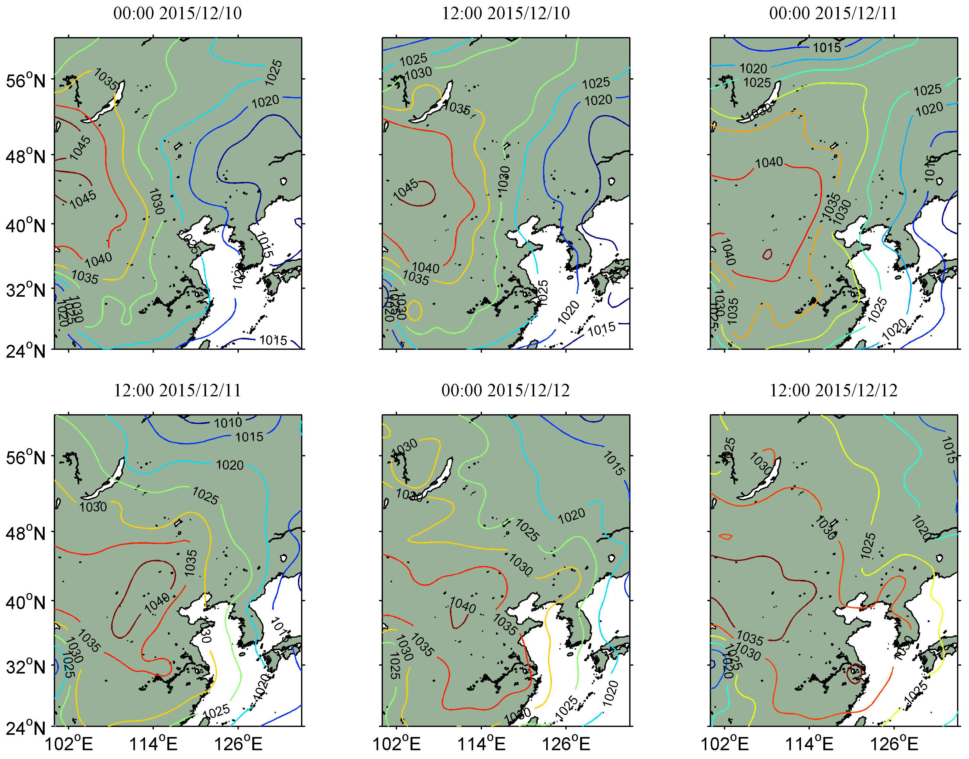
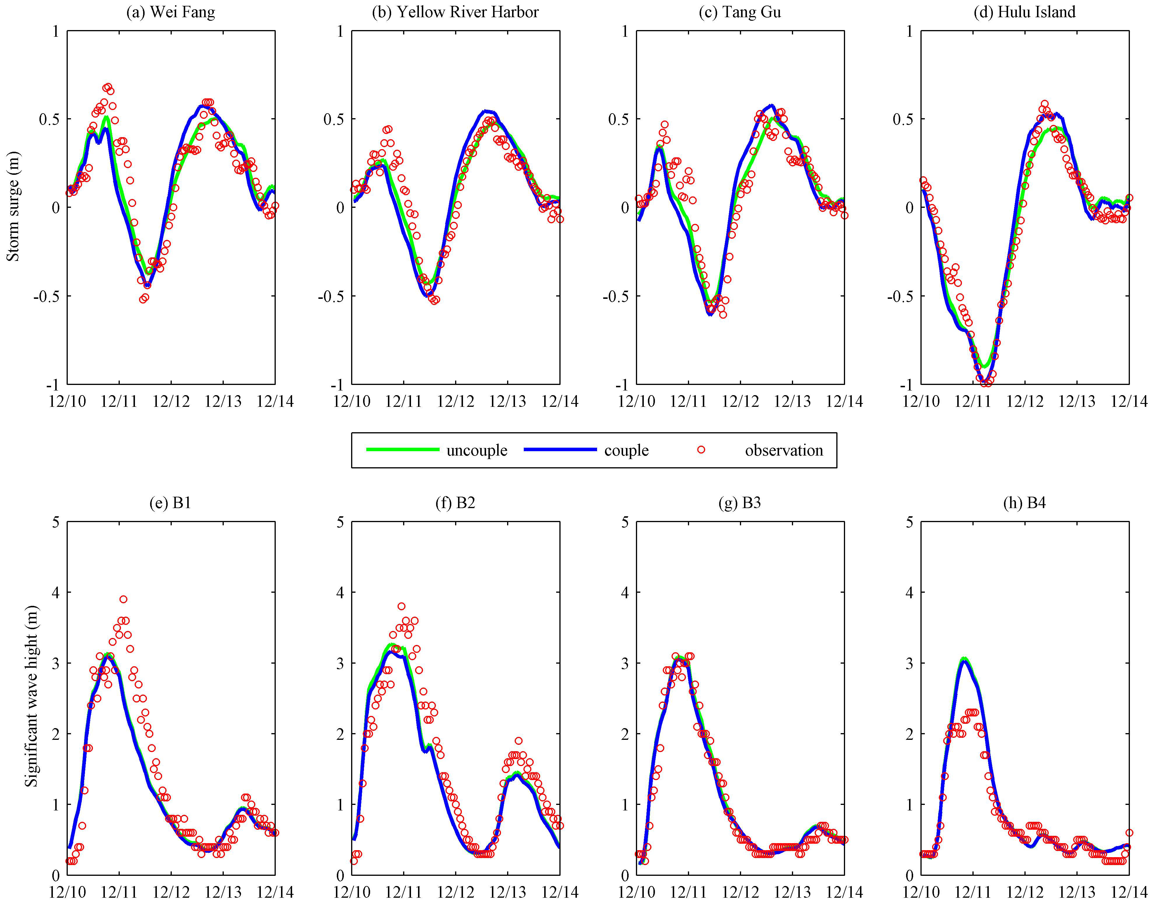
From 10 to 12 December 2015, a cold high occurred in eastern Siberia, with the central strength of 1049.5 hPa (Figure 5). The horizontal cold front passed through the NECS and induced a GNE wind. The wind field strengthened rapidly, and the maximum wind speed reached 8 on the Beaufort scale, lasting for more than 24 h. Because there is no low-pressure system in the south for coordination, the CAO-induced wind in this event had a lower wind speed and shorter wind duration than the event described in Section 3.1, so the induced storm surges and waves were relatively weak. Comparisons between the simulations and observations of the storm surge and SWHs are presented in Figure 6. The MRE, RMSE, and CC between the uncoupled and coupled simulations and observations for the tidal stations and buoys are listed in

Table 3. Statistical comparisons between observations and simulations (Exp1, Exp2, and Exp5) during the CAO-induced GNE wind.

Tidal Stations and Buoys	Latitude (° N)	Longitude (° E)	MRE		RMSE (m)		CC
			Exp1 or Exp2	Exp5	Exp1 or Exp2	Exp5	Exp1 or Exp2	Exp5
Wei Fang	-	-	15%	3.6%	0.13	0.16	0.90	0.85
Yellow River Harbor	-	-	18%	5.4%	0.096	0.13	0.93	0.90
Tang Gu	-	-	11%	0.49%	0.12	0.15	0.92	0.89
Hulu Island	-	-	11%	2.4%	0.09	0.11	0.98	0.97
B1	38.02	119.51	20%	21%	0.42	0.44	0.93	0.93
B2	39.30	120.36	14%	17%	0.36	0.38	0.94	0.94
B3	38.09	121.04	0.45%	1.6%	0.16	0.17	0.98	0.98
B4	38.55	123.20	34%	32%	0.29	0.28	0.98	0.98

MRE represents the relative error of the extreme values in the time series of simulation; RMSE represents the root-mean-square error between the time series of observation and the time series of simulation; CC represents the correlation coefficient between the time series of observation and the time series of simulation.

. The inclusion of wave–current interactions improved the simulation of positive storm surge but caused very small changes to the waves. On the analysis scale of this study, the impact of wave–current interactions on surface waves during CAOs was insignificant.

In the two CAO events, simulation of the storm surge was good but significant error existed in the SWH simulation, especially in the second event. In Figure 6, the peaks are underestimated by 0.5 m to 1 m at B1 and B2, and overestimated by 0.5 m at B4. The locations of B1 and B2 were close to the Long Kou station, which can be used for reference. As shown in Figure 2, the CFSR wind speed was smaller than the observed data from Long Kou and the SWHs at B1 and B2 were underestimated, indicating that the simulation of waves was greatly affected by the accuracy of the wind field. This conclusion is also reflected in the possible high value of wind speed difference in the West Korea Bay on the incomplete satellite image, which resulted in the overestimated SWHs at B4 (Figure 2h). In this situation, the simulation results of the uncoupled experiments appeared to agree “better” with observations than the coupled experiments. Therefore, the simulated errors are mainly linked to errors in the wind forcing. Furthermore, the deviation between the ETOPO terrain data and the actual terrain has also affected the numerical simulations.

4. Results and Discussion

4.1. Evolutions of Storm Surge and Wave

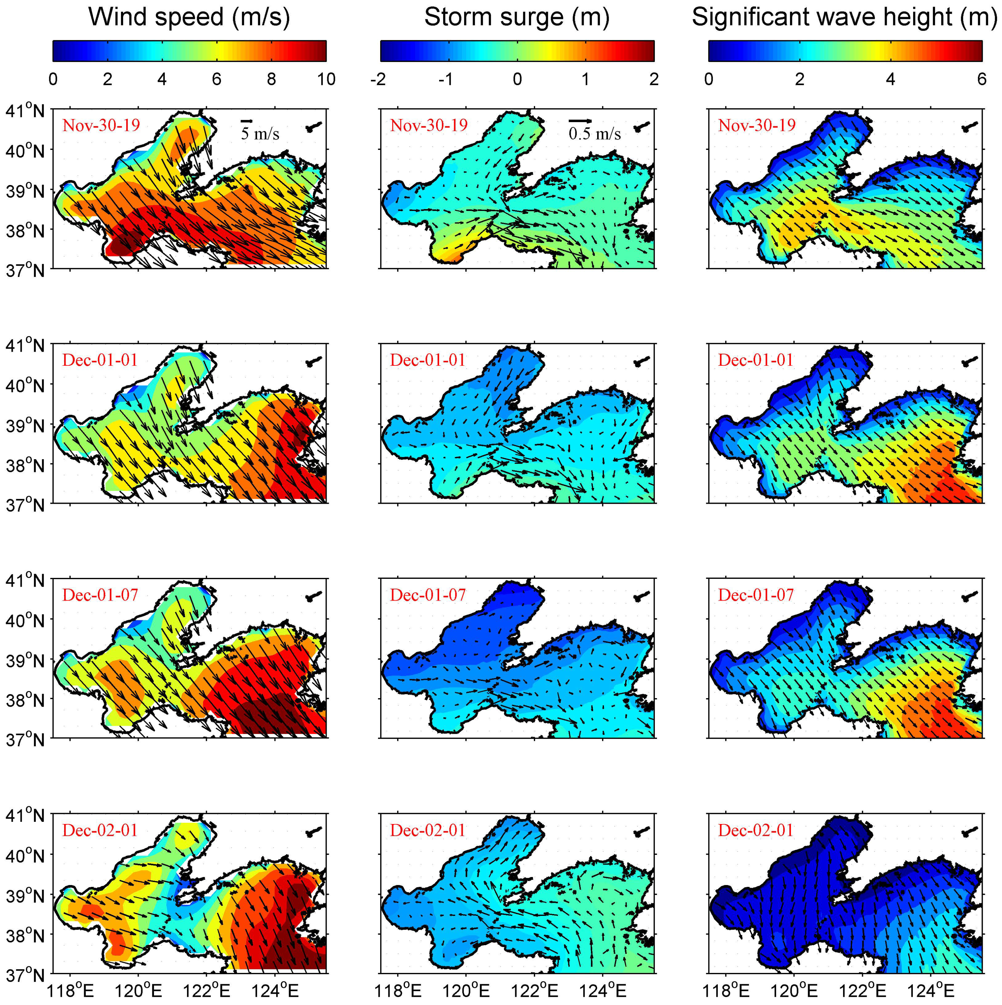
Figure 7 and Figure 8 show the evolution of storm surge, current, and waves simulated from Exp5 at certain times during the two CAO events. The wind vectors from the CFSR dataset are also shown for comparison. During the CAO-induced GNW wind, seawater initially flowed from Liaodong Bay to Bohai Bay, Laizhou Bay, and the northern Yellow Sea, producing a positive storm surge as high as 1.3 m at 19:00 on November 30. This surge was located primarily in the southeast top of Laizhou Bay. In addition, an extreme area of SWH, with a maximum exceeding 3 m, appeared in the center of the Bohai Sea. Subsequently, the sustained northwest winds brought a significant negative surge to the Bohai Sea, where the current velocity reached a maximum of 1.4 m/s at 20:00 on 30 November. The SWHs reached a maximum >6 m at 01:00 on 1 December, and the extreme region moved to the center of the Yellow Sea. Negative surge appeared sequentially from north to south. The maximum negative storm surge reached 1.7 m at 07:00 on 1 December. As the wind subsided, the sea level returned to normal by virtue of the pressure gradient force, and the SWHs decreased.

In the second CAO event, seawater flowed from Liaodong Bay to the southwest, resulting in a positive storm surge in Bohai Bay and Laizhou Bay. The water level contours were perpendicular to the wind directions. The maximum positive surge reached up to 0.6 m at 18:00 on 10 December and the maximum negative surge reached 1.3 m at 05:00 on 11 December. As the wind weakened, seawater returned from the Yellow Sea to the Bohai Sea, and the current velocity reached a maximum of 0.85 m/s at 14:00 on 11 December. The low-frequency fluctuation in the NECS at the end of CAO was the result of the pumping oscillation of seawater between the NECS and the southern Yellow Sea induced by the GNE wind. The maximum SWHs, exceeding 4 m at 21:00 on 10 December, occurred in the central areas of the Bohai Sea and northern Yellow Sea.

4.2. Contributions of Wave–Current Interaction to Water Level and Current

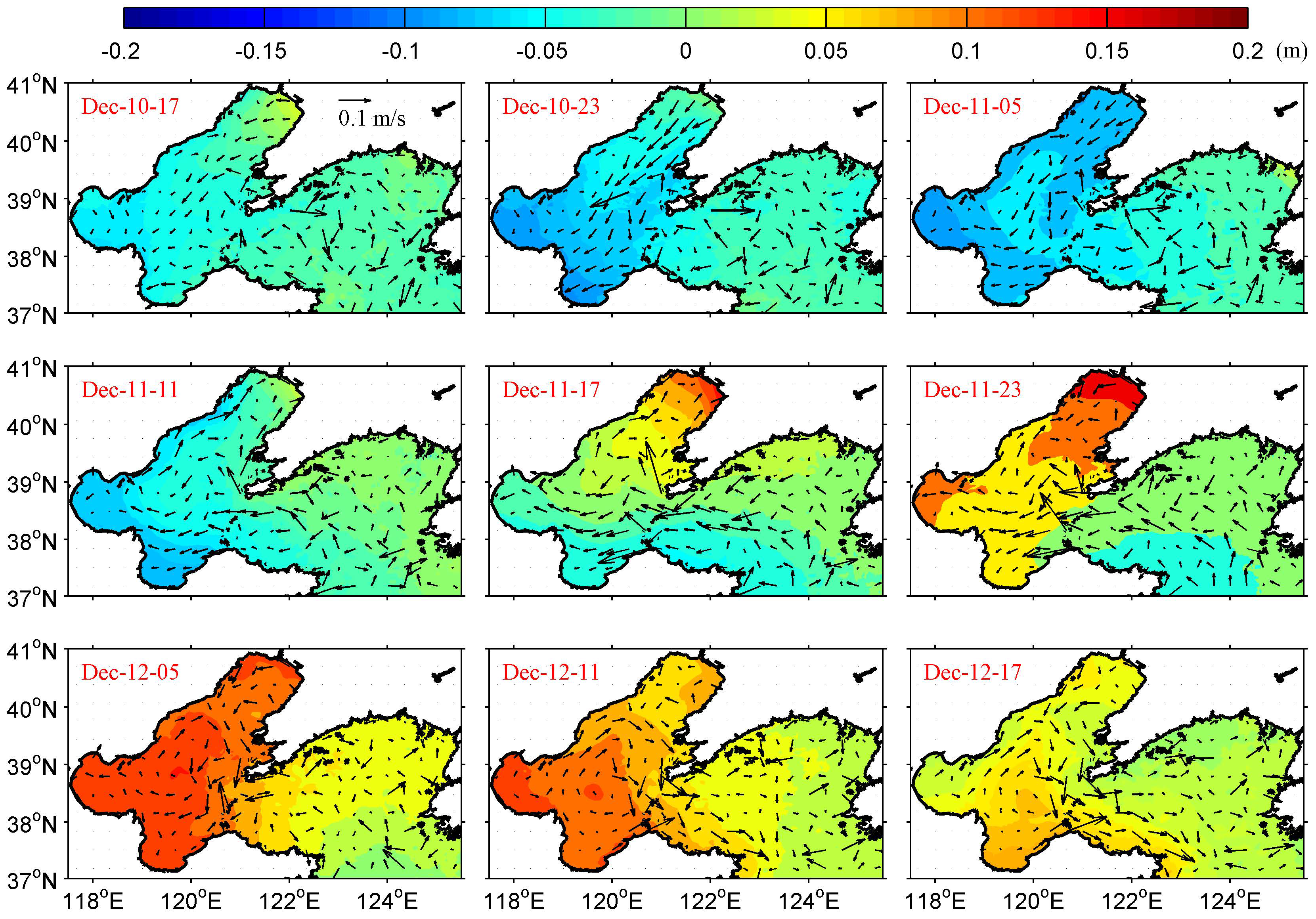
Wave set-up (or set-down), one of the most prominent characteristics of wave–current interactions, can be estimated by the storm surge difference between Exp1 and Exp5. The evolution of storm surge difference and barotropic current field difference when considering waves during the two events is shown in Figure 9 and Figure 10. The contribution of wave–current interactions to the water elevation exhibited a significant spatiotemporal variation in the NECS. During the CAO-induced GNW wind, the variation of surge difference, which ranged from −0.40 to 0.20 m, was consistent with the storm surge in the NECS. The maximum set-up created by the waves occurred at the end of the CAO, while the maximum set-down created by the waves occurred at 05:00 on 1 December. The maximum wave-forced current velocity was 0.50 m/s, which occurred at 13:00 on 1 December. During the CAO-induced GNE wind, the wave modulation in the storm surge ranged from −0.30 to 0.30 m, and the maximum wave-forced current velocity was 0.40 m/s. The maximum surge difference and the maximum wave-forced current velocity both occurred at the end of the CAO.

A comparison of the occurrence times of the storm surges, waves, and wave set-ups during CAOs revealed that the wave set-up (including set-down; the same hereafter) occurred earlier than the storm surge because the wave field responded to the wind field more quickly. When strong waves propagated to the coastal water zone, the wave set-up was pronounced and diminished as the waves weakened. When the currents transported the waters and kinetic energy to the Yellow Sea, the wave height increased, and a negative surge difference was induced. In the nearshore area, the wind field and wave height decreased, whereas the storm surge and its difference induced by the wave effect increased noticeably. Because of the superimposed pressure gradient force, the direction of the wave-forced current corresponded to the storm surge difference, and the area of strong wave-forced current was consistent with the area of significant surge difference in both events. Moreover, when the wave directions were close to the current directions, the wave effect enhanced the intensity of the storm surges; otherwise, the wave effect weakened the intensity. Therefore, during CAOs, wave modulations in the storm surge and current were closely related to the difference between the wave and current directions.

According to Chen et al. [54], the surge induced by wave was up to 0.55 m due to the giant typhoon generated waves and the steep sea-bottom slope in the northeastern coast of Taiwan. As reported by Parvathy and Bhaskaran [55], waves propagating on a steeper slope will have a severer energy dissipation over a narrower surf zone as compared to those on a gentler slope. Because of the gentle slope of NECS, the wave breaks early in the offshore and deforms gradually towards the shore [56]. Therefore, the contribution of the wave to the storm surge largely depends on the sea floor slope. In addition, the intensity of the storm, or the magnitude of the wave height, plays a role in the contribution of the wave to the surge [57].

4.3. Contributions of Wave–Current Interaction to Waves

It has been recognized that waves are influenced by the current effect in two main ways: (1) spatiotemporal change of water level; and (2) spatiotemporal change of current field. The dominant factors for the current effect modulation of the wave are different under different dynamic conditions [58]. In the northwest Pacific Ocean, some researchers attributed this modulation to the change of water level [59,60]; some other researchers attributed the modulation to the change of water level for nearshore and the change of current field for offshore [58]. In fact, storm surge affects the water depth in the wave calculation and changes the deformation process of nearshore waves. Therefore, it has a great impact on nearshore wave breaking. In addition, previous studies have shown that wave heights increase when waves and currents are in opposite directions; otherwise, they decrease [61].

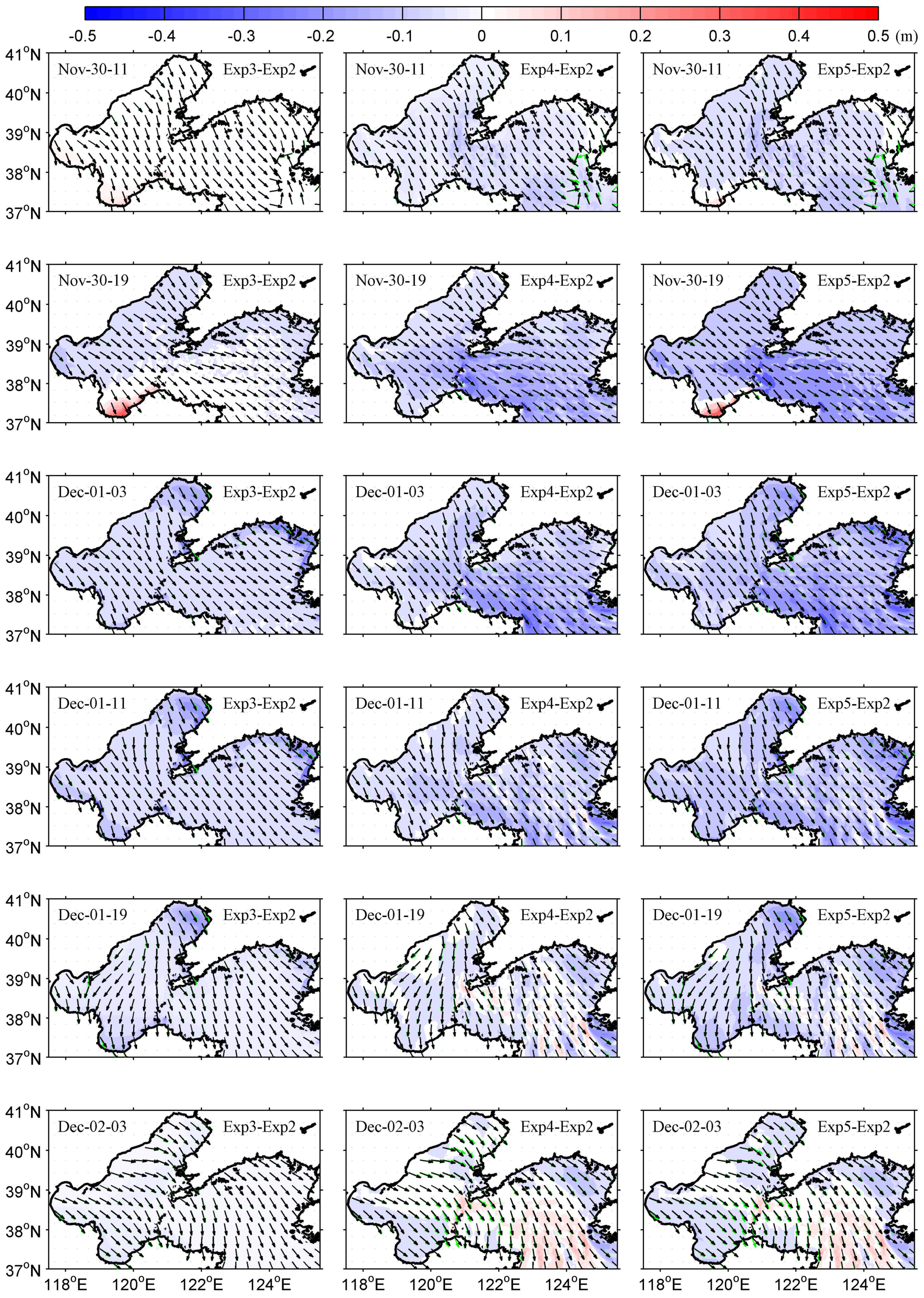
The results of Exp5−Exp2 revealed the evolutions of the SWH difference and mean wave direction change induced by the superimposed effect of the water level and current field changes (Figure 11 and Figure 12). During the CAO-induced GNW wind, the SWH difference ranged from −0.50 to 0.40 m. The maximum negative SWH difference occurred at the head of Liaodong Bay and West Korea Bay at 02:00 on 1 December. The maximum positive SWH difference occurred at the head of Laizhou Bay at 19:00 on 30 November. During the CAO-induced GNE wind, the SWH difference ranged from −0.30 to 0.30 m. A negative SWH difference was induced in most areas, especially in the Liaodong Bay and central seas, with extreme values occurring at 01:00 on 11 December.

The results of Exp3−Exp2 and Exp4−Exp2, which, respectively, revealed the evolution of the SWH difference and mean wave direction change induced by the water level change and the current field change in the two CAO events, are also shown in Figure 11 and Figure 12. In the nearshore seas, the severe storm surge resulted in a greater impact on wave height from water level changes than from currents. The wave heights in the areas with positive storm surge, such as Laizhou Bay, increased markedly and the wave heights in the areas with negative storm surge, such as Liaodong Bay, decreased markedly. In some areas, such as the head of Laizhou Bay, the effects of storm surge and current field on the wave height were opposed: a positive storm surge increased the wave height, whereas a current moving in the wave direction reduced the wave height. In the open sea, current modulation of the wave height was related to the current field and varied with the terrain.

Our data indicated that the wave–current interaction on wave direction simulation was negligible, a finding similar to that of Fan et al. [28]. Mean wave directions were modulated as much as 20° and 40°, mainly in the initial and final stages of CAOs. Model simulations with and without wave–current interactions demonstrated that the modulation of wave direction was primarily due to the current field and not to the storm surge. When the wave–current direction difference was larger, the magnitude of the wave direction modulation was greater, such as the cases that occurred in the bay heads and the Bohai Strait. The data proved that the wave–current direction difference had a significant influence on changes in water level and wave parameters.

4.4. Wave Effect on the Momentum Balance

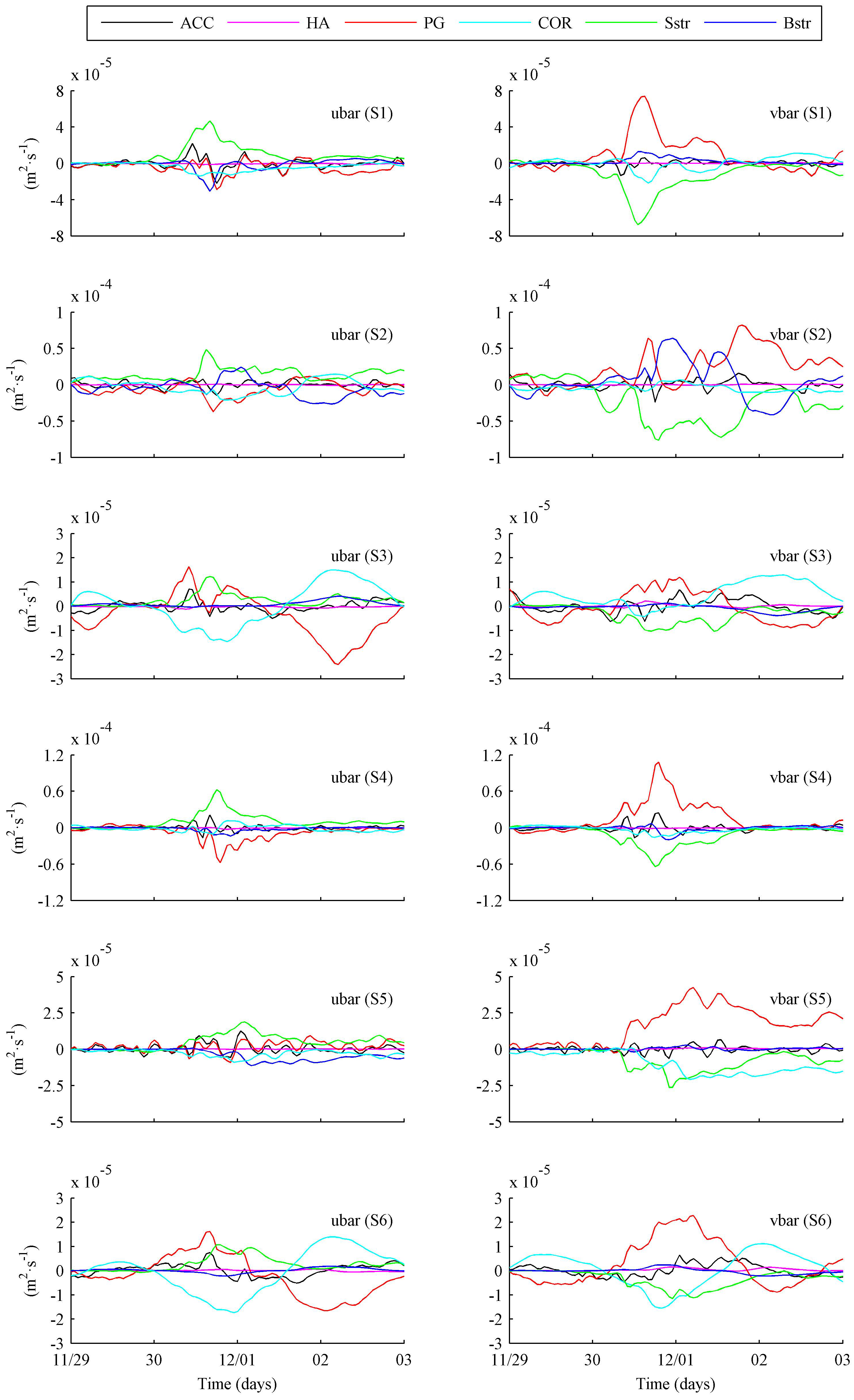
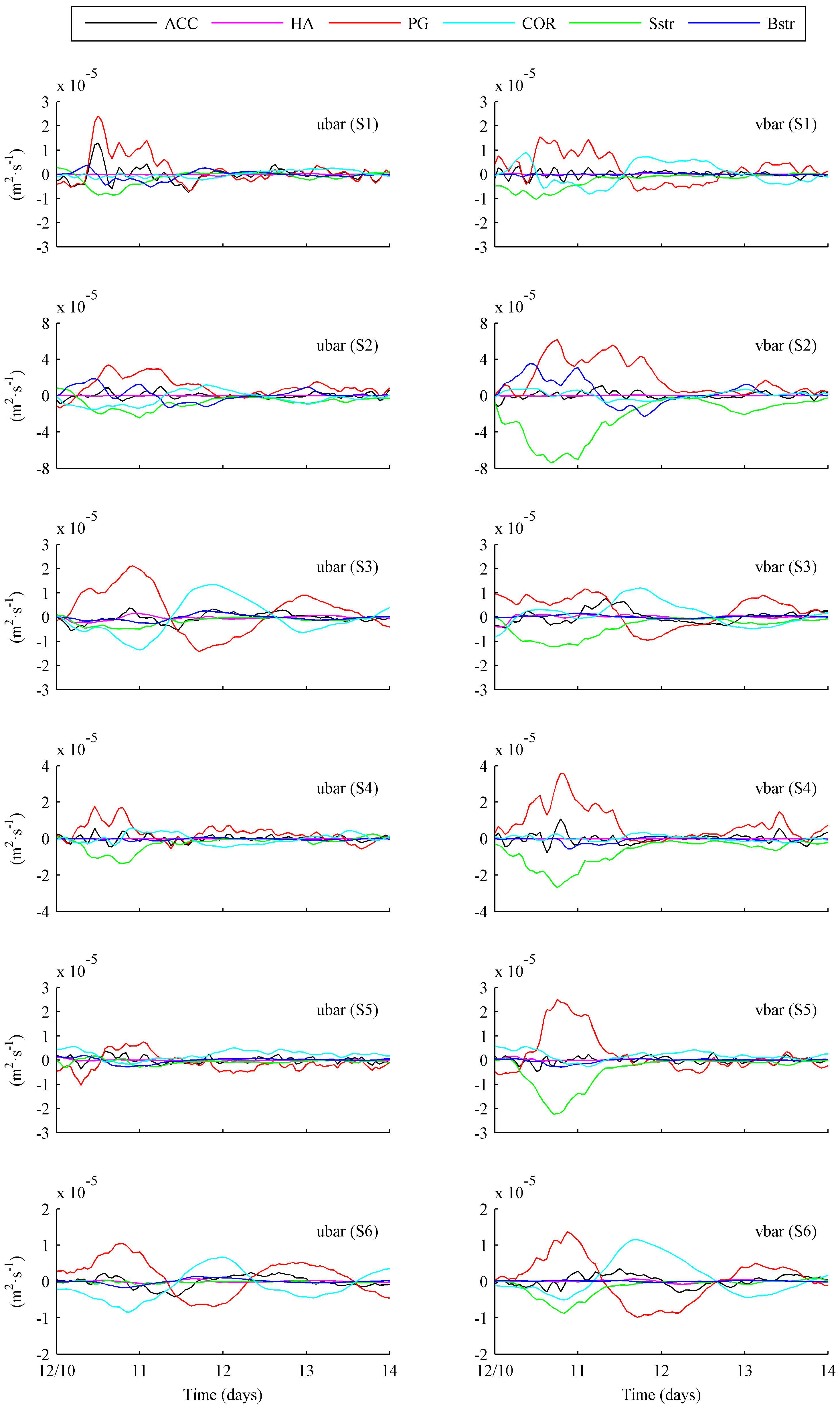
We selected six sites (S1–S6) in the NECS (Figure 1) and the terms in the vertically integrated momentum balance equation, including the x- and y-directions, were calculated separately for Exp1 and Exp5. Figure 13 and Figure 14 show the time series of momentum balance terms, including HA, PG, COR, Sstr, and Bstr, in Exp1 at S1–S6 during the two CAOs. Among the momentum terms, the largest contributions in both experiments were from the PG and Sstr. The Bstr did not create significant changes in most areas during CAOs, with the exception of some coastal locations, such as S2. The directions of the PG, Sstr, and Bstr were consistent with the storm surge spatial variations, the wind directions, and the bottom current directions. The momentum balance followed the geostrophic balance more closely in the open water than in the nearshore waters. Because of the low current velocity during CAOs in the NECS, the HA lost importance in the momentum balance.

Previous studies have calculated various terms of the momentum balance and highlighted changes in the momentum balance caused by waves. Our results agreed with the previous findings that the largest contribution was from the PG [45,62]. Prakash and Pant [62], however, reported that the Bstr was also a leading term during a tropical cyclone. The Bstr increased when the apparent bed roughness was enhanced by waves, possibly because, during tropical cyclones, the wave heights are much greater than during CAOs, and the waves can reach the sea bottom. In addition, the advective acceleration is a dominant term of the momentum balance in the pure tidal case [45]. Therefore, the dominant term of momentum balance is different for different meteorological systems and marine background environments.

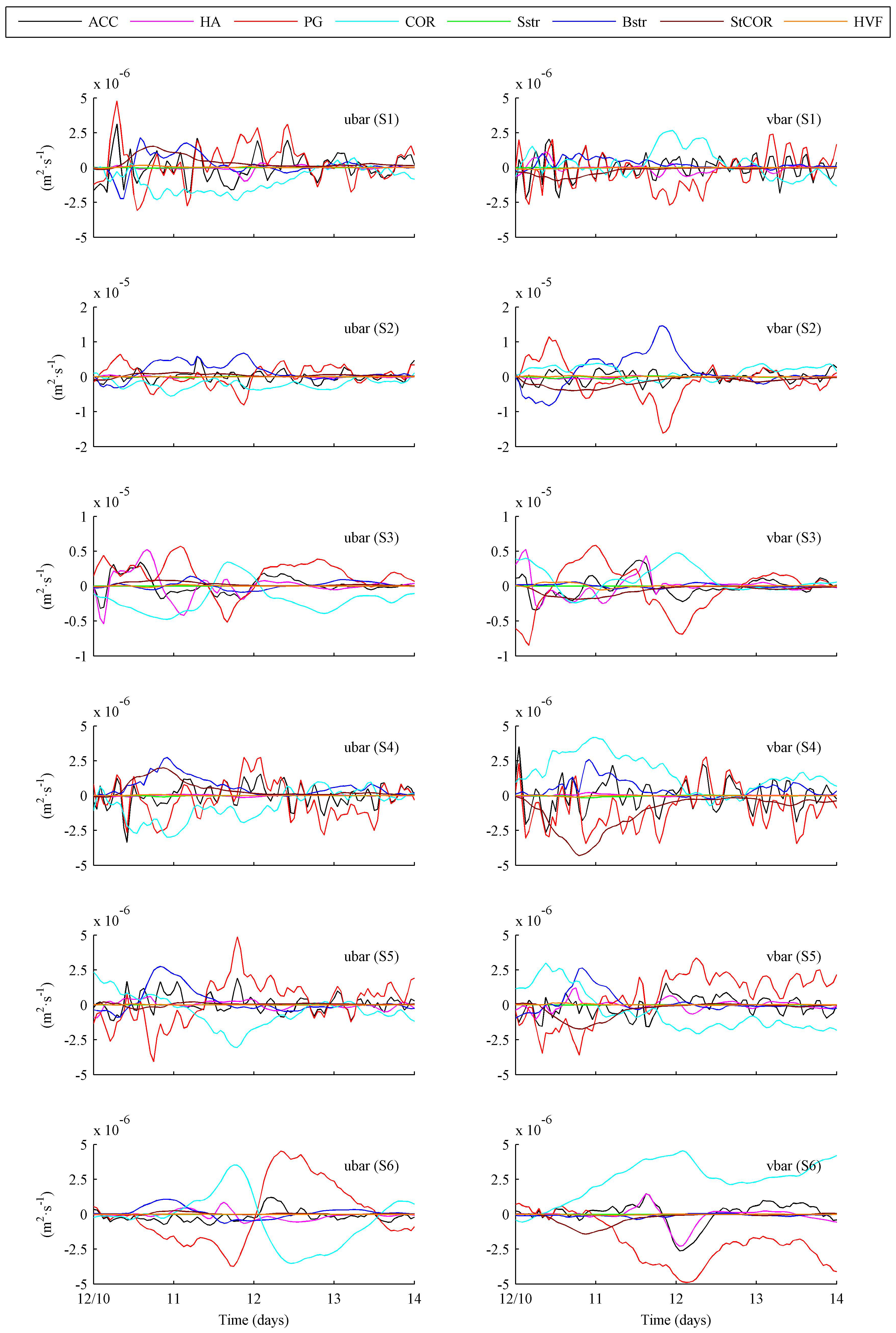
Some previous studies [63,64] have shown that the wave effect on currents can be achieved in the following three ways: (1) by increasing the surface roughness, which further increases the surface stress; (2) by increasing the bottom stress due to the shallow water depth; and (3) by inducing three-dimensional wave forces. Figure 15 and Figure 16 are plots of time series of the differences in contributory terms (HA, PG, COR, Sstr, Bstr, StCOR, and HVF) of the momentum balance with the inclusion of waves in the coupled model at sites S1–S6 during the two CAOs. The momentum balance difference varied significantly in time and space and vacillated between positive and negative values. In all regions, the PG exhibited the largest changes in response to waves. The superimposed PG controlled the direction of the wave-forced current. The inclusion of waves resulted in a considerable enhancement in the magnitude of the COR and HA, particularly in the open waters. Note that the COR differences maintained a balance with the PG differences. The Bstr differences, whose directions were basically the same as the wave-induced current field, displayed their maximum values at the heads of the four bays. Prakash and Pant [62] also reported that the inclusion of waves resulted in a considerable enhancement in the magnitude of the PG and Bstr terms, particularly in shallow regions. The StCOR differences, with a single peak of increasing and then decreasing values, were significant in the coastal waters. The differences in the Sstr and HVF were at least one order of magnitude smaller than those of the other terms.

4.5. Current Effect on the Wave Action Balance

The wave action balance was influenced by the current effect in several ways. First, Equations (13)–(16) indicated that the current variation induced the advection, refraction, and wavenumber shift of waves in spatial and spectral spaces [65]. Second, the surface wind velocity vector was replaced by the difference between the surface current vector and the surface wind velocity vector, manifested as the relative wind effect [15]. Third, the currents changed the sea surface roughness and further modulated surf breaking and whitecapping [66]. Fourth, in the shallow water of the NECS, the storm surge modified the water depth and changed the bottom friction of the waves.

Figure 17 illustrates the time series of all the energy balance term differences caused by the current effect during the two CAOs at sites S1–S6. The responses of the wave action balance terms varied with the current velocity both spatially and temporally. Overall, the GenWind and DisWcap differences, which had similar trends, were the most significant of all the terms. When the wave–current direction difference was small, the relative wind effect reduced the energy input to waves and induced less whitecapping, and vice versa. DisBot increased and decreased markedly with negative and positive storm surges, respectively. DisSurf decreased because of the current effect in shallow coastal waters, where the waves preferentially break. Wave PropXY (current-induced wave advection), PropSigma (wavenumber shift), and PropTheta (wave refraction) differences were related to the vector sum of wave velocity and current velocity, the gradient of current velocity along the wave direction, and the gradient of current velocity perpendicular to the wave direction, respectively. In general, PropXY difference was more significant than PropSigma and PropTheta differences. PropTheta was enhanced in open waters and reduced in coastal waters, whereas PropSigma was enhanced in open waters (e.g., S3 and S6) but almost unchanged in coastal waters. Finally, the difference in TranCur was much smaller than the differences in the other terms.

Wang and Sheng [33] examined wave–current interactions during three severe weather events. In the case of fast-moving hurricanes, the dominant mechanisms of the wave–current interaction on waves included current-induced modification of GenWind, PropXY, and PropTheta. In the case of a slow-moving winter storm, the effect of the wave–current interaction on waves depended mainly on GenWind and PropXY. The weather system characteristics of the CAO event were similar to the winter storm event and the results were consistent. Unfortunately, previous studies did not discuss the dissipation terms in the wave action balance and cannot be compared with the related results of this study.

Because of the 5 m limiting depth and the coarse resolution of nearshore regions in the model configuration, this study did not consider wave evolution and dissipation in shallow, nearshore regions. Therefore, the noted findings are limited only to open, deep-water conditions and cannot be generalized to nearshore regions.

5. Conclusions

We assessed the impact of nonlinear wave–current interactions on marine dynamic environment factors (such as sea level, current velocity, and wave height) over the NECS during CAOs using CFSR wind field data and the COAWST coupled modeling system. Quantitative estimates for two representative case studies were presented. When the CAO-induced currents and waves met, significant momentum and energy exchanges occurred. The wave effect—which intensified the storm surge—superimposed the pressure gradient force and further induced the residual current. This effect was found to be closely related to the difference between wave direction and current direction. The pressure gradient difference due to the wave effect was more significant than the other momentum balance terms. The bottom stress difference, which mainly occurred in coastal waters, was much larger than the surface stress difference and the induced vortex force. The effects of currents on waves occurred primarily in shallow coastal areas, such as the heads of bays, during times of pronounced storm surge. The differences in the wave energy balance terms caused by the current effect were found to be strongly related to the vectors of wave velocity and current velocity. In particular, the energy generation due to wind input, the energy dissipation due to whitecapping, and the wave advection all changed significantly in the NECS.

This study filled a gap in our understanding of wave–current interaction during CAOs in the open ocean of the northern East China Sea, away from the coastline. In an upcoming study, we will include more meteorological systems to explore the similarities and differences in the impact of the wave–current interactions on storm surges and waves during tropical cyclones, extratropical cyclones, and CAOs.

References

- Ricchi, A.; Miglietta, M.M.; Falco, P.; Benetazzo, A.; Bonaldo, D.; Bergamasco, A.; Sclavo, M.; Carniel, S. On the use of a coupled ocean–atmosphere–wave model during an extreme cold air outbreak over the Adriatic Sea. Atmos. Res. 2016, 172–173, 48–65. [Google Scholar] [CrossRef]
- Feng, J.; Li, D.; Li, Y.; Liu, Q.; Wang, A. Storm surge variation along the coast of the Bohai Sea. Sci. Rep. 2018, 8, 11309. [Google Scholar] [CrossRef] [PubMed] [Green Version]
- Mo, D.; Hou, Y.; Liu, Y.; Li, J. Study on the growth of wind wave frequency spectra generated by cold air outbreaks in the northern East China Sea. J. Oceanol. Limnol. 2018, 36, 1509–1526. [Google Scholar] [CrossRef]
- McInnes, K.L.; Hubbert, G.D. A numerical modeling study of storm surges in Bass Strait. Aust. Meteorol. Mag. 2003, 52, 143–156. [Google Scholar]
- Zhao, P.; Jiang, W. A numerical study of storm surges caused by cold-air outbreaks in the Bohai Sea. Nat. Hazards 2011, 59, 1–15. [Google Scholar] [CrossRef]
- Yao, Q.; Zheng, C.W.; Su, Q.; Wang, J.; Liang, X.Y.; Li, Y.B. Simulation of wave field in the China Sea by using WAVEWATCH III wave model. Mar. Forecast. 2013, 30, 49–54, (In Chinese with English Abstract). [Google Scholar]
- Benetazzo, A.; Carniel, S.; Sclavo, M.; Bergamasco, A. Wave-current interaction: Effect on the wave field in a semi-enclosed basin. Ocean Model. 2013, 70, 152–165. [Google Scholar] [CrossRef]
- Li, X.; Dong, S. A preliminary study on the intensity of cold wave storm surges of Laizhou Bay. J. Ocean Univ. China 2016, 15, 987–995. [Google Scholar] [CrossRef]
- Wang, K.; Hou, Y.; Li, S.; Du, M.; Chen, J.; Lu, J. A comparative study of storm surge and wave setup in the East China Sea between two severe weather events. Estuar. Coast. Shelf Sci. 2020, 235, 106583. [Google Scholar] [CrossRef]
- Bonaldo, D.; Antonioli, F.; Archetti, R.; Bezzi, A.; Correggiari, A.; Davolio, S.; De Falco, G.; Fantini, M.; Fontolan, G.; Furlani, S.; et al. Integrating multidisciplinary instruments for assessing coastal vulnerability to erosion and sea level rise: Lessons and challenges from the Adriatic Sea, Italy. J. Coast. Conserv. 2019, 23, 19–37. [Google Scholar] [CrossRef]
- Ji, C.; Zhang, Q.; Wu, Y. An empirical formula for maximum wave setup based on a coupled wave-current model. Ocean Eng. 2018, 147, 215–226. [Google Scholar] [CrossRef]
- Lane, E.M.; Restrepo, J.M.; Mcwilliams, J.C. Wave–Current Interaction: A Comparison of Radiation-Stress and Vortex-Force Representations. J. Phys. Oceanogr. 2007, 37, 1122–1141. [Google Scholar] [CrossRef] [Green Version]
- Kumar, N.; Voulgaris, G.; Warner, J.C.; Olabarrieta, M. Implementation of the vortex force formalism in the coupled ocean-atmosphere-wave-sediment transport (COAWST) modeling system for inner shelf and surf zone applications. Ocean Model. 2012, 47, 65–95. [Google Scholar] [CrossRef]
- Zhang, C.; Hou, Y.; Li, J. Wave-current interaction during Typhoon Nuri (2008) and Hagupit (2008): An application of the coupled ocean-wave modeling system in the northern South China Sea. J. Oceanol. Limnol. 2018, 36, 663–675. [Google Scholar] [CrossRef]
- Ardhuin, F.; Roland, A.; Dumas, F.; Bennis, A.C.; Sentchev, A.; Forget, P.; Wolf, J.; Girard, F.; Osuna, P.; Benoit, M. Numerical wave modeling in conditions with strong currents: Dissipation, refraction, and relative wind. J. Phys. Oceanogr. 2012, 42, 2101–2120. [Google Scholar] [CrossRef]
- Hopkins, J.; Elgar, S.; Raubenheimer, B. Observations and model simulations of wave-current interaction on the inner shelf. J. Geophys. Res. 2016, 121, 198–208. [Google Scholar] [CrossRef] [Green Version]
- Donelan, W.; Dobson, F.; Smith, S. On the dependence of sea surface roughness on wave development. J. Phys. Oceanogr. 1993, 23, 2143–2149. [Google Scholar] [CrossRef] [Green Version]
- Kang, K.; Iorio, D.D. Depth- and current-induced effects on wave propagation into the Altamaha River Estuary, Georgia. Estuar. Coast. Shelf Sci. 2006, 66, 395–408. [Google Scholar] [CrossRef]
- Zhang, X.F.; Han, G.J.; Wang, D.X.; Li, W.; He, Z.J. Effect of surface wave breaking on the surface boundary layer of temperature in the Yellow Sea in summer. Ocean Model. 2011, 38, 267–279. [Google Scholar] [CrossRef]
- Deng, Z.; Xie, L.; Yu, T.; Shi, S.; Jin, J.; Wu, K. Numerical study of the effects of wave-induced forcing on dynamics in ocean mixed layer. Adv. Meteorol. 2013, 2013, 365818. [Google Scholar] [CrossRef]
- Singh, S.K.; Raushan, P.K.; Debnath, K. Combined effect of wave and current in rough bed free surface flow. Ocean Eng. 2018, 160, 20–32. [Google Scholar] [CrossRef]
- Zheng, J.; Tang, Y. Numerical simulation of spatial lag between wave breaking point and location of maximum wave-induced current. China Ocean Eng. 2009, 23, 59–71. [Google Scholar]
- Dietrich, J.C.; Zijlema, M.; Westerink, J.J.; Holthuijsen, L.H.; Dawson, C.; Luettich, R.A., Jr.; Jensen, R.E.; Smith, J.M.; Stelling, G.S.; Stone, G.W. Modeling hurricane waves and storm surge using integrally-coupled, scalable computations. Coast. Eng. 2011, 58, 45–65. [Google Scholar] [CrossRef]
- Teles, M.J.; Pires-Silva, A.A.; Benoit, M. Numerical modelling of wave current interactions at a local scale. Ocean Model. 2013, 68, 72–87. [Google Scholar] [CrossRef]
- Zhang, J.-S.; Zhang, Y.; Jeng, D.-S.; Liu, P.L.-F.; Zhang, C. Numerical simulation of wave–current interaction using a RANS solver. Ocean Eng. 2014, 75, 157–164. [Google Scholar] [CrossRef]
- Xie, L.; Pietrafesa, L.J.; Wu, K. A numerical study of wave–current interaction through surface and bottom stresses: Coastal ocean response to Hurricane Fran of 1996. J. Geophys. Res. 2003, 108, 1–31. [Google Scholar] [CrossRef] [Green Version]
- Xu, F.; Perrie, W.; Toulany, B.; Smith, P.C. Wind-generated waves in Hurricane Juan. Ocean Model. 2007, 16, 188–205. [Google Scholar] [CrossRef]
- Fan, Y.; Ginis, I.; Hara, T.; Wright, C.W.; Walsh, E.J. Numerical simulations and observations of surface wave fields under an extreme tropical cyclone. J. Phys. Oceanogr. 2009, 39, 2097–2116. [Google Scholar] [CrossRef]
- Wu, L.; Rutgersson, A.; Sahlée, E. Upper-ocean mixing due to surface gravity waves. J. Geophys. Res. 2015, 120, 8210–8228. [Google Scholar] [CrossRef] [Green Version]
- Gong, W.; Chen, Y.; Zhang, H.; Chen, Z. Effects of Wave–Current Interaction on Salt Intrusion during a Typhoon Event in a Highly Stratified Estuary. Estuaries Coasts 2018, 41, 1904–1923. [Google Scholar] [CrossRef]
- Sun, Y.; Perrie, W.; Toulany, B. Simulation of wave-current interactions under hurricane conditions using an unstructured-grid model: Impacts on ocean waves. J. Geophys. Res. 2018, 123, 3739–3760. [Google Scholar] [CrossRef]
- Hsiao, S.C.; Wu, H.L.; Chen, W.B.; Chang, C.H.; Lin, L.Y. On the Sensitivity of Typhoon Wave Simulations to Tidal Elevation and Current. J. Mar. Sci. Eng. 2020, 8, 731. [Google Scholar] [CrossRef]
- Wang, P.; Sheng, J. A comparative study of wave-current interactions over the eastern Canadian shelf under severe weather conditions using a coupled wave-circulation model. J. Geophys. Res. 2016, 121, 5252–5281. [Google Scholar] [CrossRef]
- Fan, Y.; Ginis, I.; Hara, T. Momentum flux budget across the air–sea interface under uniform and tropical cyclone winds. J. Phys. Oceanogr. 2010, 40, 2221–2242. [Google Scholar] [CrossRef]
- Liu, G.; Perrie, W.; Hughes, C. Surface wave effects on the wind-power input to mixed layer near-inertial motions. J. Phys. Oceanogr. 2017, 47, 1077–1093. [Google Scholar] [CrossRef]
- Sun, Y.; Chen, C.; Beardsley, R.C.; Xu, Q.; Qi, J.; Lin, H. Impact of current-wave interaction on storm surge simulation: A case study for Hurricane Bob. J. Geophys. Res. 2013, 118, 2685–2701. [Google Scholar] [CrossRef] [Green Version]
- Marsooli, R.; Orton, P.M.; Mellor, G.; Georgas, N.; Blumberg, A.F. A coupled circulation–wave model for numerical simulation of storm tides and waves. J. Atmos. Ocean. Technol. 2017, 34, 1449–1467. [Google Scholar] [CrossRef]
- Chen, Y.; Chen, L.; Zhang, H.; Gong, W. Effects of wave-current interaction on the Pearl River Estuary during Typhoon Hato. Estuar. Coast. Shelf Sci. 2019, 228, 106364. [Google Scholar] [CrossRef]
- Perrie, W.; Tang, C.L.; Hu, Y.; DeTracy, B.M. The impact of waves on surface currents. J. Phys. Oceanogr. 2003, 33, 2126–2140. [Google Scholar] [CrossRef]
- Kolstad, E.W.; Bracegirdle, T.J.; Seierstad, I.A. Marine cold-air outbreaks in the North Atlantic: Temporal distribution and associations with large-scale atmospheric circulation. Clim. Dyn. 2009, 33, 187–197. [Google Scholar] [CrossRef]
- Papritz, L.; Pfahl, S.; Sodemann, H.; Wernli, H. A Climatology Outbreaks and Their Impact on Air–Sea Heat Fluxes in the High-Latitude South Pacific. J. Clim. 2015, 28, 342–364. [Google Scholar] [CrossRef]
- Mo, D.; Hou, Y.; Li, J.; Liu, Y. Study on the storm surges induced by CAOs in the northern East China Sea. J. Mar. Syst. 2016, 160, 26–39. [Google Scholar] [CrossRef]
- Guo, Y.; Wang, Q.; Gao, W. Analysis on the impact of a cold wave on the East China Sea in January 2009. Mar. Forecast. 2010, 27, 44–47. (In Chinese) [Google Scholar]
- Warner, J.C.; Armstrong, B.; He, R.; Zambon, J.B. Development of a coupled ocean-atmosphere-wave-sediment transport (COAWST) modeling system. Ocean Model. 2010, 35, 230–244. [Google Scholar] [CrossRef] [Green Version]
- Olabarrieta, M.; Warner, J.C.; Kumar, N. Wave-current interaction in Willapa Bay. J. Geophys. Res. Ocean. 2011, 116, 1–27. [Google Scholar] [CrossRef] [Green Version]
- Olabarrieta, M.; Warner, J.C.; Armstrong, B.; Zambon, J.B.; He, R. Ocean-atmosphere dynamics during Hurricane Ida and Nor’Ida: An application of the coupled ocean-atmosphere-wave-sediment transport (COAWST) modeling system. Ocean Model. 2012, 43, 112–137. [Google Scholar] [CrossRef] [Green Version]
- Shchepetkin, A.F.; McWilliams, J.C. The regional oceanic modeling system (ROMS): A split-explicit, free-surface, topography-following-coordinate oceanic model. Ocean Model. 2005, 9, 347–404. [Google Scholar] [CrossRef]
- Booij, N.R.; Ris, R.C.; Holthuijsen, L.H. A third-generation wave model for coastal regions: 1. Model description and validation. J. Geophys. Res. Ocean. 1999, 104, 7649–7666. [Google Scholar] [CrossRef] [Green Version]
- Uchiyama, Y.; McWilliams, J.C.; Shchepetkin, A.F. Wave-current interaction in an oceanic circulation model with a vortex-force formalism: Application to the surf zone. Ocean Model. 2010, 34, 16–35. [Google Scholar] [CrossRef]
- Carvalho, D.; Rocha, A.; Gómez-Gesteira, M.; Santos, C.S. Comparison of reanalyzed, analyzed, satellite-retrieved and NWP modelled winds with buoy data along the Iberian Peninsula coast. Remote Sens. Environ. 2014, 152, 480–492. [Google Scholar] [CrossRef]
- Colberg, F.; McInnes, K.L. The impact of future changes in weather patterns on extreme sea levels over southern Australia. J. Geophys. Res. Ocean. 2012, 117, 1–19. [Google Scholar] [CrossRef] [Green Version]
- Chen, W.B.; Chen, H.; Hsiao, S.C.; Chang, C.H.; Lin, L.Y. Wind forcing effect on hindcasting of typhoon-driven extreme waves. Ocean Eng. 2019, 188, 106260. [Google Scholar] [CrossRef]
- Hsiao, S.C.; Chen, H.; Chen, W.B.; Chang, C.H.; Lin, L.Y. Quantifying the contribution of nonlinear interactions to storm tide simulations during a super typhoon event. Ocean Eng. 2019, 194, 106661. [Google Scholar] [CrossRef]
- Chen, W.B.; Lin, L.Y.; Jang, J.H.; Chang, C.H. Simulation of Typhoon-Induced Storm Tides and Wind Waves for the Northeastern Coast of Taiwan Using a Tide–Surge–Wave Coupled Model. Water 2017, 9, 549. [Google Scholar] [CrossRef]
- Parvathy, K.G.; Bhaskaran, P.K. Wave attenuation in presence of mangroves: A sensitivity study for varying bottom slopes. Int. J. Ocean Clim. Syst. 2017, 8, 126–134. [Google Scholar] [CrossRef] [Green Version]
- Song, H.; Kuang, C.; Gu, J.; Zou, Q.; Liang, H.; Sun, X.; Ma, Z. Nonlinear tide-surge-wave interaction at a shallow coast with large scale sequential harbor constructions. Estuar. Coast. Shelf Sci. 2020, 233, 106543. [Google Scholar] [CrossRef]
- Wu, G.; Shi, F.; Kirby, J.T.; Liang, B.; Shi, J. Modeling wave effects on storm surge and coastal inundation. Coast. Eng. 2018, 140, 371–382. [Google Scholar] [CrossRef]
- Song, H.; Kuang, C.; Wang, X.H.; Ma, Z. Wave-current interactions during extreme weather conditions in southwest of Bohai Bay, China. Ocean Eng. 2020, 216, 108068. [Google Scholar] [CrossRef]
- Kang, K.; Kim, S. Wave-tide interactions during a strong storm event in Kyunggi Bay, Korea. Ocean Eng. 2015, 108, 10–20. [Google Scholar] [CrossRef]
- Yu, X.; Pan, W.; Zheng, X.; Zhou, S.; Tao, X. Effects of wave-current interaction on storm surge in the Taiwan strait: Insights from typhoon Morakot. Cont. Shelf Res. 2017, 146, 47–57. [Google Scholar] [CrossRef]
- Jia, Y.; Yin, B.; Yang, D. A numerical study of the influence of wave-current interaction on water elevation and significant wave height in the East China Sea. Mar. Sci. 2009, 33, 82–86, (In Chinese with English Abstract). [Google Scholar]
- Prakash, K.R.; Pant, V. On the wave-current interaction during the passage of a tropical cyclone in the Bay of Bengal. Deep Sea Res. Part II 2020, 172, 104658. [Google Scholar] [CrossRef]
- Yin, B.; Sha, R.; Yang, D.; Cheng, M. Numerical study of wave-tide-surge coupling processes. Studi. Mar. Sin. 2006, 47, 1–15. [Google Scholar]
- Xie, L.; Liu, H.; Peng, M. The effect of wave-current interactions on the storm surge and inundation in Charleston Harbor during Hurricane Hugo 1989. Ocean Model. 2008, 20, 252–269. [Google Scholar] [CrossRef]
- Holthuijsen, L.H.; Tolman, H.L. Effects of the Gulf Stream on Ocean Waves. J. Geophys. Res. 1991, 96, 12755–12771. [Google Scholar] [CrossRef]
- Shi, L.; Olabarrieta, M.; Valle-Levinson, A.; Warner, J.C. Relevance of wind stress and wave-dependent ocean surface roughness on the generation of winter meteotsunamis in the Northern Gulf of Mexico. Ocean Model. 2019, 140, 101408. [Google Scholar] [CrossRef]
Figure 1.
(a) Geographic location of East China Sea (including Bohai Sea and Yellow Sea) in the northwest Pacific Ocean, and the model domain of the coupled model (red dashed box). (b) A zoomed-in view of the model domain and the corresponding bathymetry showing tidal stations (black triangles), buoys (blue squares for the cold air outbreak (CAO) event in 2014, and green squares for the CAO event in 2015), and chosen sites (red circles). The black dashed lines separate the Bohai Sea, the northern Yellow Sea, and the southern Yellow Sea.
Figure 2.
(a–d) Time series of CFSR (blue lines) and ERA5 (black lines) wind velocity in comparison with the observed (red circles) wind velocity at Long Kou and Hu Lu Dao during the two representative events; (e–h) wind velocity difference (m/s) between CFSR and ASCAT product at validity time.
Figure 3.
Evolution of mean sea level pressure (hpa) distribution from 30 November to 1 December 2014.
Figure 4.
Comparisons between simulated and observed storm surges (a–d) and significant wave heights (e–h) during four days in late November and early December 2014 at four tidal stations along the coast and buoys B1, B2, B3, and B5: simulated in Exp1 (green lines in (a–d)) and Exp2 (green lines in (e–h)); simulated in Exp5 (blue lines); and observed (red circles).
Figure 5.
Evolution of mean sea level pressure (hpa) distribution from 10 to 12 December 2015.
Figure 6.
Comparisons between simulated and observed storm surges (a–d) and significant wave heights (e–h) from 10 to 14 December 2015, at four tidal stations along the coast and buoys B1, B2, B3, and B4: simulated in Exp1 (green lines in (a–d)) and Exp2 (green lines in (e–h)); simulated in Exp5 (blue lines); and observed (red circles).
Figure 7.
Evolution of wind speed, wind direction, storm surge, barotropic current, significant wave height, and mean wave direction distributions at certain times during the CAO-induced GNW wind.
Figure 8.
Evolution of wind speed, wind direction, storm surge, barotropic current, significant wave height, and mean wave direction distributions at certain times during the CAO-induced GNE wind.
Figure 9.
Evolution of storm surge difference (colors) and barotropic current difference (arrows) induced by the wave effect (Exp5−Exp1) during the CAO-induced GNW wind.
Figure 10.
Evolution of storm surge difference (colors) and barotropic current difference (arrows) induced by the wave effect (Exp5−Exp1) during the CAO-induced GNE wind.
Figure 11.
Evolution of significant wave height difference (colors) and mean wave direction change induced by change in water level (Exp3−Exp2), current field (Exp4−Exp2), and the combined effect (Exp5−Exp2) during the CAO-induced GNW wind. Green arrows represent the mean wave directions simulated in Exp2; black arrows represent the mean wave directions simulated in Exp3, Exp4, or Exp5.
Figure 12.
Evolution of significant wave height difference (colors) and mean wave direction change induced by change in water level (Exp3−Exp2), current field (Exp4−Exp2), and the combined effect (Exp5−Exp2) during the CAO-induced GNE wind. Green arrows represent the mean wave directions simulated in Exp2; black arrows represent the mean wave directions simulated in Exp3, Exp4, or Exp5.
Figure 13.
Time series of vertically integrated momentum balance terms (Exp1) in the x- and y-directions at six sites (S1–S6) during the CAO-induced GNW wind.
Figure 14.
Time series of vertically integrated momentum balance terms (Exp1) in the x- and y-directions at six sites (S1–S6) during the CAO-induced GNE wind.
Figure 15.
Time series of vertically integrated momentum balance term differences (Exp5–Exp1) in the x- and y-directions at sites S1–S6 during the CAO-induced GNW wind.
Figure 16.
Time series of vertically integrated momentum balance term differences (Exp5–Exp1) in the x- and y-directions at sites S1–S6 during the CAO-induced GNE wind.
Figure 17.
Time series of energy balance term differences (Exp5–Exp2) at sites S1–S6 during the CAO-induced GNW wind (a–f) and GNE wind (g–l).