
A Review and Meta-Analysis of Underwater Noise Radiated by Small (<25 m Length) Vessels


1
Australian Institute of Marine Science, Perth, WA 6009, Australia
2
Centre for Marine Science & Technology, Curtin University, Bentley, WA 6102, Australia
*
Author to whom correspondence should be addressed.
J. Mar. Sci. Eng. 2021, 9(8), 827; https://doi.org/10.3390/jmse9080827
Submission received: 13 July 2021
/
Revised: 25 July 2021
/
Accepted: 27 July 2021
/
Published: 30 July 2021
(This article belongs to the Special Issue Ocean Noise: From Science to Management)
Abstract
:Managing the impacts of vessel noise on marine fauna requires identifying vessel numbers, movement, behaviour, and acoustic signatures. However, coastal and inland waters are predominantly used by ‘small’ (<25 m-long) vessels, for which there is a paucity of data on acoustic output. We reviewed published literature to construct a dataset (1719 datapoints) of broadband source levels (SLs) from 17 studies, for 11 ‘Vessel Types’. After consolidating recordings that had associated information on factors that may affect SL estimates, data from seven studies remained (1355 datapoints) for statistical modelling. We applied a Generalized Additive Mixed Model to assess factors (six continuous and five categorical predictor variables) contributing to reported SLs for four Vessel Types. Estimated SLs increased through ‘Electric’, ‘Skiff’, ‘Sailing’, ‘Monohull’, ‘RHIB’, ‘Catamaran’, ‘Fishing’, ‘Landing Craft’,’ Tug’, ‘Military’ to ‘Cargo’ Vessel Types, ranging between 130 and 195 dB re 1µPa m across all Vessel Types and >29 dB range within individual Vessel Types. The most parsimonious model (22.7% deviance explained) included ‘Speed’ and ‘Closest Point of Approach’ (CPA) which displayed non-linear, though generally positive, relationships with SL. Similar to large vessels, regulation of speed can reduce SLs and vessel noise impacts (with consideration for additional exposure time from travelling at slower speeds). However, the relationship between speed and SLs in planing hull and semi-displacement vessels can be non-linear. The effect of CPA on estimated SL is likely a combination of propagation losses in the shallow study locations, often-neglected surface interactions, different methodologies, and that the louder Vessel Types were often recorded at greater CPAs. Significant effort is still required to fully understand SL variability, however, the International Standards Organisation’s highest reporting criteria for SLs requires water depths that often only occur offshore, beyond the safe operating range of small vessels. Additionally, accurate determination of monopole SLs in shallow water is complicated, requiring significant geophysical information along the signal path. We suggest the development of appropriate shallow-water criteria to complete these measurements using affected SLs and a comprehensive study including comparable deep- and shallow-water measures.
1. Introduction
It is globally accepted that anthropogenic noise is an acute and chronic stressor of marine taxa that can alter marine soundscapes on multiple temporal, frequency and spatial scales, disrupting the acoustic characteristics of ecosystems [1,2]. The sound emitted by vessels under power (particularly large ships; [3]) is a key component of this noise and the size of the commercial shipping fleet has been growing year on year [4]. Vessel noise has been shown to increase stress levels, alter behaviour, displace individuals and mask communication in marine mammals, fish, and invertebrates at multiple life stages, potentially leading to population consequences, e.g., [5,6,7,8,9,10,11,12,13,14,15,16,17]. Thus, minimising the exposure of marine fauna to vessel noise is likely to have significant benefits for the global marine ecosystem.
Modelling of instantaneous and cumulative sound exposure levels at any given location requires knowledge of the number of vessels, the level of noise produced by each and understanding their different operations. There are several potential sources of noise emitted by individual vessels, but oscillating bubbles produced by sheet and vortex cavitation near the turning propeller dominate the acoustic output, emitting acoustic energy at frequencies related to diameter range of the bubbles [18,19,20,21,22]. These levels can be broadly estimated from a selection of engineering coefficients including the cavitation number (a function of size, speed, blade number, and depth of the propeller as well as environmental factors), block coefficient (a function of vessel length, breadth, and draft), and Admiralty coefficient (a function of vessel power, speed, and displacement) [18]. However, these values are rarely, if ever, reported in bioacoustics literature and for broader application, it may be more prudent to consider the individual contributing characteristics (e.g., power, displacement and speed), rather than the coefficients themselves (e.g., Admiralty coefficient). In addition, although cavitation contributes significant energy to the broadband level, it is not the sole source of noise, otherwise electric vessels would offer limited noise reduction.
Significant effort has been invested in characterising the sounds of large ships and understanding the potential drivers of source levels see [6,19,20,21,22], which have been principally related predominantly to the size and speed of the vessel in the bioacoustics literature [19]. There are, however, little data publicly available on the source levels of small (classed here as <25 m length) vessels and no comprehensive analysis linking the different vessel types within this size class to understand how different vessel characteristics contribute to the acoustic signature.
Anthropogenic noise around offshore shipping lanes is dominated by large (>25 m) commercial ships, whereas shallower coastal waters and inland waterways also host to many smaller vessels that are more variable in speed and highly mobile. These small vessels often traverse spatially controlled areas (e.g., vessel channels) and can have very shallow drafts (<1 m) so they can operate in waters as shallow as <2 m depth, positioning them close to sessile, sedentary or site-attached taxa [11,23,24]. Despite multiple sources of anthropogenic noise in these waters, such as personal watercraft (jetskis), planes, helicopters, unmanned aerial vehicles (drones), swimmers, surfers, scuba divers, and increasingly, remotely operated underwater vehicles, etc., e.g., [25,26,27,28,29], the daytime soundscapes of this habitat are often dominated by the sounds of small vessels, e.g., [30,31].
Small vessels have many applications and designs vary significantly from planing to displacement hulls, single or multiple hulls, using one or more inboard or outboard engines of varying power. Flat (planing) hulls are designed to quickly rise out of the water with increasing speed until the boats skim along the surface at high speed, rather than pushing the water aside (e.g., skiffs, rigid hull inflatable boats {RHIBS}). Displacement hulls are round-bottomed, ploughing through the water and buoyed by the water the hull displaces (e.g., landing craft, cargo vessels). Semi-displacement hulls, such as fishing vessels and mono- or multi-hull cruisers, are a combination of the two hull types and displace water at low speeds, but able to semi-plane at cruising speeds. Thus, their acoustic signature and broadband source level may vary significantly with vessel design and operation.
2. Definitions and Scope
This study reviews the available published literature on noise emitted by small vessels and conducts a meta-analysis of data from studies that provide a source level estimate, matched with additional information about factors that contribute to variance in the acoustic output. We have considered three types of measure to quantify the broadband acoustic levels at a nominal 1 m range:
- Radiated noise levels (abbreviation: RNL; symbol: LRN), defined as the level of the product of the distance d from a ship reference point of a sound source and the far-field root mean-square sound pressure prms at that distance for a specified reference value. The RNL is computed as:
- 2.
- Monopole source levels (abbreviation: MSL; symbol: LSL), defined as the mean-square sound pressure level at a distance of 1 m from a hypothetical monopole source, placed in a hypothetical infinite lossless medium. The MSL is determined by adding the propagation loss NPL to the mean-square sound pressure level Lp2 measured at some range d:
- The propagation loss NPL is determined through modelling (e.g., a parabolic equation model), accounting for the effects of the local environment at the time.
- 3.
- Environment-affected source levels (abbreviation: ASL; symbol: LASL), defined as the mean-square sound pressure level at a distance of 1 m in a natural environment (i.e., with existing surface boundaries) and thus affected by the local environment at the time. The ASL is determined by linear regression of the mean-square sound pressure level measured at a series of ranges.
The first two of these measures are defined in the International Standards Organisation (ISO) standards 17208 (parts 1 and 2) to measure and report noise levels of vessels in deep water [32,33]. However, the highest standard of ISO criteria to measure radiated noise of vessels requires hydrophones to be positioned at vertical incidence angles of 15°, 30°, and 45° to the vessel at a minimum (slant) range of 100 m (i.e., 70 m water depth) in waters depths of a minimum of 150 m [32,33]. Such minimum depth and 45° elevation requirements cannot be achieved in many coastal situations and might involve potentially unsafe operations for some small vessels as they would require travelling significant distances offshore. Additionally, without accurate knowledge of the geophysical characteristics of the seafloor, propagation losses modelled during the estimation of MSLs can be misleading, particularly at low (tens to low hundreds of hertz) frequencies [31]. As a result, some reports provide ASLs determined from linear regression of numerous recordings taken at multiple ranges from a vessel to empirically model the dipole source signal, as it is affected by the shallow waters and interactions with water and seabed surfaces, e.g., [31,34].
3. Objectives
The aim of our study was to improve our understanding of driving factors and variance in noise emission by small vessels, which we achieved through the following objectives:
- Identify studies that provide broadband source level estimates for individual small vessels, together with appropriate vessel specifications, operations and environmental data.
- Access supplementary data from these studies (i.e., additional recordings of vessels that were available but not included in the publication, but meet the same standards of quality as those reported).
- Collate data from (1) and (2) to identify potentially influential common factors that were reported alongside the estimated source levels and produce a dataset from which a statistical model can be developed to identify their contribution to variance in those estimates. This is not a model to predict noise from small vessels, but to tease out the drivers of variation in the available reported data.
- Compare and characterise the inter-study variability in methodologies and reported source levels.
- Review and describe the various factors that are known to contribute to variations in the vessel spectra and estimated source levels and, where data are available, quantify their contribution to the variance.
Completing these objectives will reconcile all the informative available data previously reported on small vessel source levels in the bioacoustics literature. It will provide a better understanding into the factors driving estimated source levels recorded in real-world conditions and assist in setting regulations that may limit the levels of noise to which nearby aquatic fauna are subjected. It will also provide a qualitative assessment of the impacts the use of different sites, equipment and methodologies have on the estimation of acoustic signatures.
4. Materials and Methods
To provide an element of continuity, we have followed similar methodologies for gathering data and statistical analysis as Chion et al. [19] in their evaluation of large commercial vessels. To produce a dataset that encompassed as many individual estimates of source levels of small vessels as possible we have:
- Conducted a literature review using Google Scholar and Scopus to search for papers that included “vessel” or “boat” AND “source level” OR “sound signature” OR “acoustic signature” OR “noise signature” OR “radiated noise” in the title or keywords;
- Assessed citations found within these publications to see if they met the required criteria for inclusion in the dataset (described below) even though they were missed in the original search;
- Included data from publications that provided a broadband source level estimate in the dataset;
- Only included reported values of individual vessel passes and not aggregated assessments of the source levels in the dataset for statistical modelling;
- Examined previous reports authored by the investigators of this study that met the criteria below for additional recordings that were not included in the original publication, but were collected under the same standard and protocols as those in the publication. Available data were added to the overall dataset.
The estimated source levels for all samples in the dataset were grouped into 11 vessel types (Table 1) and logged with all pertinent information provided in the report. Specifically, intrinsic (originating from the vessel’s own static and dynamic characteristics) and extrinsic (data collection, types of propagation model applied, and the environment affecting the recordings) factors [19] that have been previously shown to contribute to vessel source spectra were recorded (Table 2). An initial assessment found that several of these factors (from here called ‘predictor’ variables) were rarely reported and were discarded from consideration in statistical modelling, thus only recordings that provided information on the bulk of the remaining factors were retained.
This dataset comprised 1719 recordings of individual passes from 224 vessels, with 1 to 349 passes of any individual vessel. The remaining intrinsic and extrinsic factors were defined as either categorical predictor variables (including Vessel type (11 levels), Hull type (3 levels), Vessel ID, Propagation model (3 levels), and Reference (8 levels—each individual study)) or continuous predictor variables (Vessel length, Speed, Engine power, Water depth, Hydrophone depth, closest point of approach (CPA), and CPA/Hydrophone depth) [35].
Speed has been reported as a significant predictor of variation in ship source level, e.g., [19,21,36]. Therefore, as an initial test, linear regression of speed and source level of the entire dataset were investigated in the form of:
where SL is the source level (RNL, MSL or ASL, dB re 1 µPa m), Cv is the velocity coefficient, v is the vessel velocity (kn), vr is a reference velocity (1 kn) and k is the intercept.
An issue with multi-variate analysis is the potential for correlation between predictor variables [35], of which there are several in Table 2 that could intuitively be related. Visual data exploration was conducted to display outliers and aid the testing of collinearity of covariates based on variance inflation factors (VIFs). To avoid including collinear variables, covariates with a VIF > 3 were not added to the model [35,37]. During this assessment, the following observations and actions were made:
- Vessel Type, Length and Hull Type displayed collinearity. Source level displayed a relationship with speed that appeared to vary with vessel type. Further, hull type was reduced to two levels after accounting for missing values. As a result, vessel type was chosen over length and hull type.
- Water Depth and Hydrophone Depth were highly collinear. Water Depth provided a greater range of values to describe variation than Hydrophone Depth. Additionally, the Closest Point of Approach (CPA) was often significantly large with respect to the Hydrophone Depth, and therefore provided a variable that describes the impact of the largest interference pattern, the Lloyd’s mirror effect, on source level that could otherwise be explained by hydrophone depth. Therefore, Water Depth was retained for the model and Hydrophone Depth was discarded.
- Propagation Model showed collinearity with Vessel Type, Water Depth and Engine Power and was not included in the model.
Engine Power data displayed imbalance amongst Vessel Types (VIF = 3), therefore, the validity and interpretation of any models that included both variables was assessed with care. We applied generalised additive mixed models (GAMMs) with a Gaussian distribution and identity link function for continuous data to investigate the factors driving estimated source levels of small vessels. GAMMs were chosen to enable the inclusion of smoothing splines (smoothers) in the model, as data exploration revealed a non-linear effect of log10(speed), which was supported by similar observations found in previous reports, e.g., [31,38]. GAMMs also allow the inclusion of random effects to account for dependencies in the data [35]. Such a model allows investigation of the factors influencing the reported source level. However, as there are intrinsic and extrinsic factors driving the variance in estimated levels, the model was not designed to predict noise from vessels.
For inclusion in the model, the estimated source level required associated data on all chosen variables, which was not always available. Further, each tested level within the model required >20 data points to provide enough information [44] and so those levels of variables with <20 data points were not included. To allow the function to calculate the random intercept, av, on more than a single observation, and to avoid an unbalanced random effect, we also decided to only include vessels that had been recorded at least three times. As a result, the following data points and resulting categories were removed from the dataset:
- Engine Power and/or CPA was not reported for 226 data points, which were excluded, removing all data from the Military and Cargo Vessel Types.
- Fishing and Tug Vessel Types only contained 16 and 8 measurements, respectively, that had data on Engine Power, whereas Landing Craft originally only included 8 data points, thus these Vessel Types were not included in the model.
- Data exploration showed that the Vessel Speed and CPA data collected for Electric and Sailing vessels were skewed (e.g., only one electric vessel, recorded multiple times at one speed and one CPA). Therefore, these two levels, with <23 data points each, did not contain enough information to produce sensible smoothers and were not included in the model.
- Several studies reported only one or two measurements for individual vessels (e.g., Veirs and Veirs [3]) and had to be removed.
- In the remaining datasets, a total of 64 data points were present for vessels that were recorded less than three times and were not included in the final dataset.
- Additionally, four CPA outliers, which appeared to be influential data points, were also removed, two from Monohulls and two from RHIB vessel types.
The resulting full model comprised Vessel Type, Speed, CPA, Water Depth and Engine Power as fixed effects. As Speed and CPA displayed non-linear effects on source level during data exploration, these two factors were included as variable effects with smoothing splines (Table 3). Preliminary plots also suggested that the effects of Speed on source level were dependent on Vessel Type. Therefore, the smoothers for speed were added to the model separately for each Vessel Type to investigate these individual relationships, i.e., allowing different speed profiles for each Vessel Type. Vessel ID and Reference were added as random effects to account for dependencies in the data, i.e., to model the correlation between all source levels reported for the same vessels, as well as different vessel types within particular studies. This was designed to account for the risk that observations from an individual vessel (or reference) may be more similar to each other than when compared to observations from different vessels (or references), in part due to the varying sample sizes per vessel and reference. Models were fitted with the gamm4 package in R [45], as it allows the inclusion of nested random effects.
4.1. Model Validation
Model construction and validation started with the most complex model [37,46,47], which included all selected and available independent effects that may have driven variations in source level estimates, based on prior knowledge. Pearson residuals were plotted versus fitted values to validate the model, ensuring no obvious pattern was left unaccounted for. Pearson residuals were also plotted against each covariate in the model and each available covariate not in the model to ensure the model assumption of homogeneity was valid [37,47]. Generalised additive models (GAMs) were also applied to the Pearson residuals, used as the response variable, to check for nonlinear patterns left in each of the continuous covariates. Therefore, each continuous covariate was added as a smoothing function, which was then checked for its significance. A non-significant smoother means that no nonlinear pattern is left in the residuals [47].
Following the full model that included all chosen covariates, non-significant covariates (p > 0.05) were removed in a stepwise approach, with the least significant variable first. Each subsequent model was refitted and validated after each adjustment. Models were compared using Akaike’s information criterion (AIC), where a reduction by >2 units represents an improved model [48]. All analyses and corresponding figures were produced using R version 3.6.3 [49] run through RStudio Version 1.2.5042—© 2009–2020 RStudio.
4.2. Within Study Assessments
4.2.1. Applied Frequency Band
Chion et al. [19] and McKenna et al. [21] highlighted the high levels of low-frequency (<100 Hz) noise emitted by large vessels, which has also been observed in some recordings of small vessels [38,50]. Therefore, reports that do not include these frequencies may exclude portions of the vessel’s acoustic signal. To quantify the impact of the frequency band reported, we looked at 95 example recordings from Wladichuk et al. [51] that included one-third octave band levels between 10 Hz and 63 kHz for each estimate and closely met the ISO guidelines for RNL and MSL estimation. We compared the full broadband RNL estimates for each vessel and speed with estimates for the same recording with the energy from one-third octave bands of centre frequencies between 10 Hz and 100 Hz incrementally removed from the estimate.
4.2.2. Propagation Model and Equipment Configuration
Four studies provided sufficient information to directly compare their estimates of MSL and RNL for each vessel pass. Wladichuk et al. [50,51] and Erbe [36] made recordings of vessel passing in ≈70 m of water, while Parsons et al. [52] and Parsons and Meekan [31]) reported on recordings in 4 and 8 m depths of water, respectively. Data for individual passes was accessible for all studies. Wladichuk et al. [51] also provided one-third octave band levels for both the MSL and RNL estimates, which allowed a comparison of the two approaches at the one-third octave, as well as broadband level.
Finally, we also compared the estimates reported by Erbe [36], who recorded the same vessel passes using two hydrophones positioned at two of either 5 m, 10 m and, on one occasion, 25 m water depth. In that study, MSLs were calculated using a ray tracing propagation model down to 100 Hz and RNLs were provided for each measurement.
5. Results
5.1. Characterisation of Estimates from Selected Studies
Vessel recordings were collated from 17 scientific studies, each reporting estimated source levels for between one and 66 small vessels (4.3 to 25 m in length), from between one and 349 recordings, for a total of 224 vessels (Figure 1, Table 1 and Table 4). The initial dataset comprised 1719 estimated source levels where the mean level across all reports was 170 dB re 1 µPa m (max = 195, min = 130.5, standard deviation = 7.3 dB). These studies were conducted at various locations around the world in water depths between 4 and 200 m, at ranges of 10 to 2100 m, using a variety of equipment, with source level estimates analysed across a range of frequency bands (see Table 4, for technical details of each report). The initial test of a relationship between speed and source level across all vessel types produced a velocity coefficient (Cv) of 10.4, with an intercept of 148.9.
Some of these reports modelled the vessel as monopole sources, although most backpropagated their received levels as surface-affected dipole sources (either RNLs or ASLs). Each study reported on different vessel classes, with some including a breakdown of received one-third octave band levels or source levels for each recording, others included full source spectra and some reported only a single source level value (Table 4). Richardson et al. [53] provided information on measures from Buck and Chalfont [54], Miles et al. [55], Malme et al. [56], and Green [57], though full details of their studies were not available. Seven of the assessed reports provided estimates that included data points with associated information on variables that met the criteria for inclusion in the GAMM model (see Table 4 for summary information on each report).
Several other studies have reported the characteristics of acoustic signals of small vessels, which although informative on the drivers of vessel noise, did not meet the criteria to not be included here. Some of these provided maximum and minimum source levels without the mean estimate or information on the number of individual passes, e.g., [40]; gave received levels without sufficient information to determine RNLs, e.g., [13,64]; only published individual characteristics of the signal such as directionality or intensity at specific frequencies, e.g., [39,65]; did not provide vessel length and so could not be confirmed as being from a small vessel [66]; or may have reported on a vessel that was so quiet it was not detected [67].
Across all variables, the estimated source levels generally increased through the vessel types from the electric vessel emitting the lowest levels, through the planing and then semi-displacement hulls, to the displacement hull type vessels (Figure 2). Variability within vessel types was high (Figure 2). For example, estimated levels of fishing vessels ranged from 145 to 195 dB re 1 µPa m. In fact, all vessel types with more than 20 measures displayed source level ranges of >29 dB, except the single electric vessel, which was measured at only one speed.
Model
After removing all data points that did not meet the model criteria, 1355 samples from 49 vessels and four vessel types remained for statistical analysis. The final GAMM, that produced the most parsimonious model with the lowest AIC, explained approximately 22.7% of the variation encountered in this dataset (Table 5) and followed the form:
where the response variable SLivr is the estimated source level reported for observation i, for vessel v and reported by reference r. β is the intercept, s(CPAivr) and svtype(Speedivr) are the smoothing functions representing CPA and speed at observation i of vessel v and published by reference r, respectively. svtype(Speedivr) represented the four smoothing functions describing the speed profiles of the four vessel types included in the model: Skiffs, RHIBS, Monohulls and Catamarans. The random effects αv and αr were assumed to be randomly distributed with means 0 and variances σ2v or σ2r, respectively. εivr consists of the residual noise of observation i from vessel v by reference r, and was assumed to be randomly distributed with mean 0 and variance σ2. Model validation did not indicate any issues with this final model. The final GAMM did not select Hull Type, Length, Engine Power, Water Depth, Hydrophone Depth and Propagation Model for inclusion. Potential reasons for this are described in the respective sections of the discussion.
SLivr = β + s(CPAivr) + svtype(log10(Speedivr)) + αv + αr + εivr
αv ~ N(0, σ2v)
αr ~ N(0, σ2r)
εivr ~ N(0, σ2)
Speed and CPA were significant contributors and had the greatest effects on estimated source level (Table 5). The relationship and the level of influence of Speed varied between Vessel Types, with RHIBs displaying the most variation (Table 5), but all estimated speed smoothers showed an increasing effect on source level with speed (Figure 3). Skiffs displayed a linear effect of speed on source level. In comparison, RHIBs had three local maxima at ≈3, 7 and 11 ms−1, followed by a continual increase. Monohulls increased to a local maximum at ≈6 ms−1, plateauing until ≈14 ms−1, before source levels and confidence intervals increased with speed (the latter due to the small number of data points). The estimated smoother for Catamarans increased to ≈13 ms−1 before plateauing until ≈17 ms−1, after which the confidence intervals increased significantly. The estimated smoother for CPA showed a decrease to 50 m before increasing slowly until 200 m, after which the effect plateaued (Figure 4). Other factors did not provide greater explained deviance of the effect on source level and were not chosen in the final model.
The increase in the AIC value between the model using all vessels (7186) and the one only using vessels with three or more recordings (7618) supported the use of the latter in the model to remove an unbalanced random vessel effect. The AIC values also showed that the model including random structures for vessels and references, as αv + αr, fitted the data better than the model including a nested random structure of the form αv + αv/r (AICs 7186 and 7212, respectively).
5.2. Within Study Assessments
5.2.1. Frequency Band
For the 95 examples taken from Wladichuk et al. [51], increasing the lower boundary of the frequency band used to produce MSL estimates from 10 Hz to 100 Hz led to a decrease in MSLs of up to 37 dB (Figure 5). Across all speeds and vessel types, the average decrease in MSL between measurements made with the lower boundary of 10 Hz and those using a lower boundary of 50 Hz was 9.1 dB (s.d. = 9.3, max = 27.5, min = 0), whereas the same comparison with a lower limit of 100 Hz produced a mean decrease of 11.7 dB (11.2, 37.2, 0). For individual vessel types (but across all speeds), the average difference between full broadband levels and estimates with a 100 Hz lower frequency was 0.3, 12.4, 3.5, 4.1 and 11.3 dB for Catamaran, Landing craft, Monohull, RHIB and Sailboat, respectively (n = 16, 5, 43, 20, and 11, respectively). In contrast, if the energy recorded between 20 kHz and 63 kHz is removed from the broadband estimates, this results in an average reduction of only 0.11 dB and a maximum reduction of 1 dB, i.e., energy below 100 Hz provides a significantly higher contribution to the broadband estimate than energy >20 kHz.
5.2.2. Propagation Model
Across 109 of the RNL and MSL estimates provided by Wladichuk et al. [51], in 70 m of water, the mean value of MSL minus RNL was 0.66 dB (max = 4.4, min = −3.2, s.d. = 1.1, mean of absolute difference = 0.96). However, at frequencies below 100 Hz, RNL and MSL one-third octave levels diverged with decreasing frequency with MSL levels reaching up to ≈20 dB higher than RNL levels at 20 Hz (see Figure 6, for levels from two example vessels).
Parsons et al. [52] reported a +1 dB difference between 50th percentile RNL and MSL estimates for an electric ferry (125–16,000 Hz band) and a conventional-powered ferry (400–16,000 Hz band), respectively. However, one-third octave band levels referenced to 1 m from the source displayed a +18 dB difference between 100 and 200 Hz and a −18 dB difference at 500 Hz between the MSL and RNL levels, for the same percentiles. Parsons et al. [52] also noted the troughs in propagation loss models at 100–200 Hz and 300–500 Hz, attributing some of this to a lack of available accurate information on the geophysical characteristics of the seabed at the study site, required to improve the propagation model. Parsons and Meekan [31] recorded multiple measures at multiple ranges, between 10 and 100 m, from three vessels conducting repeated transects at four different speeds, in 9 m of water. The mean difference between the 50th percentiles of broadband RNL and linear regression-modelled ASLs was 6.4 (±0.2) dB. In contrast, using linear regression models developed for each one-third octave band and then integrating the ASL band levels over the full frequency range had a mean difference between RNLs and ASLs of −3.5 (±2.6) dB. The factor behind the difference between the broadband and integrated one-third octave band source level estimates was that the mean linear regression-modelled one-third octave losses peaked at 40log10(range) at 30 Hz and had declined to 10 to 15log10(range) at frequencies above 1 kHz, compared to the modelled broadband loss at 16log10(range).
5.2.3. Hydrophone Depth
Of the measures recorded by Erbe [36] at three different water depths, the MSL estimate was 7 dB greater at 25 m depth than at 10 m (n = 1), while the RNL was 6 dB higher, for the same comparison. In comparison, the MSL estimate was 4.2 dB higher (s.d = 4.6, max = 14, min = −4) at 10 m depth than at 5 m (n = 17, shallower estimate higher twice), while the RNL was 0.5 dB higher (s.d. = 3.5, max = 6, min= −4) for the same comparison (n = 17, shallower estimate higher nine times).
6. Discussion: Variation in Small Vessel Source Levels
There are few published datasets that provide source level estimates of small vessels and even fewer that supply full spectra or breakdown of the broadband estimate into smaller bandwidths (e.g., octave or one-third octave) for individual vessel passes. The reports reviewed here span nearly 50 years of field sampling and those that included methodology and vessel data that could be used to model the factors that affect source levels were spread over the last 20 years. Consequently, the types of vessels, recordings systems and back-propagation methods applied have changed significantly across this time span and the available datasets collated in this study.
For the small vessels in the broader dataset, source level estimates varied by 65 dB, compared to the 73 dB variation observed by Chion et al. [19] in their meta-analysis of large vessels. Similar to Chion et al. [19], we found that the highest levels were reported by Allen et al. [58] and the lowest levels by Veirs and Veirs [3]. The difference between mean levels reported by these two studies was 35 dB for large vessels, compared with 20 dB for small vessels, suggesting this difference is driven by methodology. The estimates by Allen et al. [58] were not included in either model and were removed from the large vessel study as outliers and excluded from our small vessel dataset as they did not contain multiple measures of individual vessels.
6.1. Research Objective
The purpose of this study was to review and investigate factors that influence small vessel noise output, with an objective of teasing out whether there are details of vessels that can be readily accessed and commonly used by acoustic researchers and managers to assist in better modelling of marine noise in a given area. However, there is a lack of integration in the literature, between the research fields interested in understanding drivers of small-vessel source levels. Although naval architects and engineers focus on the performance with some regard to acoustic output, there is less interest in the propagation of the noise, the impact on marine fauna, or how the regulations around noise may mitigate its impact. In contrast, acousticians are primarily concerned with the propagation of the noise rather than the design specifics of how it is created, and managers are concerned with the impact of the signal mitigating it. As a result, reports of source levels authored by acousticians and propagation modellers rarely include information on ship design, such as cavitation coefficients, Admiralty numbers, or block coefficients, e.g., [3,19,20,21,22,31,34,36,38,54,55,56,58,59,62,63]. In contrast, reports focussed on vessel design often omit appropriate methodology regarding signal propagation or acknowledgment of the frequency-dependent impacts of the noise on marine fauna and information with which this can be assessed, e.g., [68,69,70,71,72]. For example, although errors in source level estimates that are caused by interference patterns, can be reduced by applying a surface reflection correction for every frequency of the spectrum measured, this is quite impractical and does not entirely remove the issue.
Collectively, all of these factors contribute to variance in the estimates of spectra and source levels from field recordings that essentially validate the models created by ship designers. However, the specifications used in design calculations are rarely reported. We therefore investigated what could be gleaned about the driving factors of small vessel noise from the information that is readily available in the literature. The application of these factors by managers and regulators do not necessarily require complicated models but may be estimated from the simplest appropriate data that can be collected on all vessels operating within the area of concern. Indeed, the ship design coefficients mostly comprise variables we have noted as required factors to better understand their impacts on noise (Table 2). Therefore, although a correlation of noise with Admiralty coefficient, propeller cavitation number, and propeller loading coefficients may be more accurate, not all of the variables required to calculate them may be accessible for all vessels. In addition, current literature on large vessels has shown that a significant proportion of the variation in noise output can be broadly estimated without knowledge of some of these specifications. We attempted to investigate their combined relationship with estimated source levels of small vessels, to better understand which factors have the biggest influence and, in doing so, found a shortfall in the information provided with typical source level reports.
While numerical methods suggest the error in RNL estimates is small [73], field data displays greater levels of variance. To reconcile this difference, a more collaborative approach is needed that includes more detailed and matched efforts between computational modelling and acquisition of validation data.
6.2. Factors That Drive Acoustic Output and Estimated Source Levels within Vessel Types
We observed increases in source level estimates across the 11 vessel types from one specifically designed to be quiet (electric-powered vessels), through those designed to skim across the water (planing hulls), to vessels that plough through the water at any speed (displacement hulls). Estimated source levels for vessels designed to have a combination of planing and displacement (semi-displacement) hulls fell roughly in between the two designs. Further, vessel type (four levels available) was chosen as a categorical predictor in the final GAMM model. Thus, while sufficient data were only available to test four Vessel Types and Hull Type was not chosen in the model (likely because it explains similar variation to vessel type) the design of the vessel is a key determinant of acoustic output.
Numerous intrinsic and extrinsic variables must be considered when estimating vessel source levels. Some of these include frequency-specific energy and thus have implications for any application that focusses on specific frequency bands. Additionally, the effect of these factors may be synergistic and a change or error in one factor may compound the effect of another increasing uncertainty in the final source level estimate.
6.2.1. Intrinsic Factors
Speed
For any vessel, if the only factor that changes is speed, then the cavitation-driving tip speed correlates with vessel speed. If other factors change, such as load in the case of tug boats, then the relationship between propeller tip speed and vessel speed changes. The small boats that were considered in our study did not experience load or other changes, and so boat speed is expected to be a good indicator of cavitation noise energy, which the statistical model confirmed. With regard to the management of boat noise (by vessel operators or government regulators), boat speed is the more readily observable parameter.
Chion et al. [19] modelled the change of source level with speed for 17 individual studies of large vessels and found that Cv, the velocity coefficient in the Cvlog10(v)-space, varied from 11.7 to 49.9. When modelled within their generalised linear mixed model, it was estimated at 15.4 for large vessels. MacGillivray et al. [20] found that a 40% speed reduction decreased MSLs by approximately 10 dB in a study of voluntary speed reduction in the number of large vessels in the Port of Vancouver. For small vessels, Wladichuk et al. [51] observed the loss coefficient ranging between 10 and 58, whereas Parsons and Meekan [31] noted a non-linear relationship with speed, but generalised an average Cv of 9.7, for three vessels of ≈6 m length. In their study, the initial test of the relationship across all datapoints (all recordings of all vessel types) produced a Cv of 10.4. Although we found a non-linear relationship between speed and source level for three of the four vessel types tested in the GAMM, all four models displayed a positive relationship between speed and source level. These relationships could be generalised as Cv coefficients of 10, 16, 11 and 8 for skiffs, RHIBS, monohulls and catamarans, respectively.
Both Erbe et al. [38] and Parsons and Meekan [31] observed non-linear relationships between source levels and speed for individual vessels of <8 m length and suggested that as speed increased and vessels moved from ploughing to planing positions, the power requirement and therefore the acoustic output decreased. In fact, as the vessel moves from a displacement to planing position, the hull and propeller rise and the noise sources become shallower. Although this reduces RNLs at low frequencies the MSLs remains the same, though the source position must be accounted for in MSL estimates. In this study, although speed displayed a linear effect on skiff source level, both RHIBs and monohull vessels displayed local maxima, suggesting that one or more vessels were contributing a ‘hump’ speed to the effect.
In addition to broadband source level, frequency content of small vessel noise has also been observed to change with increasing speed. Veirs and Veirs [3] suggested that small vessels emitted more energy at high frequencies than large vessels, and that this difference increased with speed. Parsons and Meekan [31] observed that levels of higher frequency (>1 kHz) one-third octave bands increased significantly more than lower frequency (<1 kHz) one-third octave levels as speed of three vessels increased, as was also found in selected vessels from Wladichuk et al. [51]. Even individual vessels travelling at the same speed have produced source level estimates that vary by up to 20 dB [31,38,52]. Erbe et al. [38] observed this at high speed and suggested that vessel slap contributing additional noise to the estimate was the cause as the 6.5 m length, planing vessel bounced on the water. In contrast, the difficulty of maintaining vessel speed, position and direction at slow speed (5 kmh−1, 2.7 kns) was hypothesised to cause the high variation observed by Parsons and Meekan [31], and Parsons et al. [52] attributed the variation observed in short-range (15 m) estimates of both an electric (10 m-long) and conventional (25 m-long) powered vessel to the uncertainty in position and therefore range.
As with large commercial vessels, speed is a significant driver of vessel source level and can be used as a means of mitigating the impacts of noise on taxa in shallow waters. This could be achieved through a direct reduction in the number of impacts of a single vessel travelling at a slower speed, or by facilitating the presence of a larger number of slower-moving vessels in a given area (such as a whale-watching troupe) without increasing the instantaneous exposure levels. However, the additional time spent in a given area due to slower speeds, and the resulting cumulative exposures, requires consideration. Further, the relationship between speed and source level in planing hull vessels appears more complicated than for displacement hulls and may be vessel-specific, thus a single speed limit may not be appropriate for all vessels. The findings of this study demonstrate that to fully understand the impact of speed on the source level of an individual vessel, or a vessel design type, requires a greater number of recordings of individual passes at the same speed and across a wide range of speeds than has been previously achieved.
Size and Weight
Acoustic output has been shown to have a positive relationship with length [21], beam [19] and power [31]. McCauley et al. [34] and McKenna et al. [21] observed a positive increase in source level with increasing vessel load, the latter study finding gross tonnage explained deviance in octave bands (centre frequencies) between 63 and 500 Hz. However, our dataset lacked sufficient information on beam or weight-related factors for small vessels, thus only length was analysed. Length was not included in the final GAMM in our analysis, likely due to collinearity with multiple other predictor variables. Draft is rarely reported and although this is intuitively likely to have a positive relationship with source level [34], these are generally small differences compared to large vessels (1–2 m, compared with sometimes > 10 m draft).
Propeller Specifications
The relationship between propeller specifications and emitted spectra are well documented [22] with increases in engine firing rate and propeller blade rate driving increases in the intensity and frequency of tonal components of the spectra [38]. In addition, broadband energy from propeller cavitation is one of the dominant sources of noise varying with size, shape, load (as a function of displacement, speed and power, amongst other factors) and depth [18]. However, several of these specifications are rarely reported in bioacoustics literature and therefore, could not be assessed within our model. Although these characteristics can provide vessel specific information [39,40] and increase energy over specific frequency bands, they are a function of speed. Changing the depth of the propeller (source) by a few metres, as an input parameter for propagation models, has been shown to vary MSL estimates up to 10 dB [74,75]. Small vessel propellers are typically positioned only 1–2 m below the surface (though less when planing), thus changes of a few metres depth that are possible in large vessels do not occur in small vessels. Modern vessels now have the ability to vary pitch of the propeller, however, while the ability to control trim is common in current small vessels, variable pitch control is not and there is limited publicly available data in the literature. Therefore, we have not explored the impact this may have on the noise emitted by the propeller. Propeller damage (such as chips or gauges on blades) increases cavitation and the resulting bubbles have a positive relationship with acoustic energy [22]. Indeed, in some instances, cavitation noise has been shown to be more correlated to the level of propeller damage, than cavitation number [76]. As with other characteristics, condition was not reported and could not be assessed in this study.
Engine Power and Type
The final GAMM model in this study did not select engine power or type as a significant predictor of source level. However, engine power did display an imbalance with vessel type, thus any model that had selected both variables would have required cautious consideration. This is because, in general, vessel power increases with vessel type and length, thus teasing out the exact driver is non-trivial. In previous studies of small vessels, Young and Miller [77] observed that an 18 hp engine was noisier than a 7.5-hp engine and Erbe [36] compared Evinrude 175 and 225 hp engines, also finding the larger engine to be noisier, particularly at slower speeds. Indeed, Parsons and Meekan [31] characterized the ASLs for three small vessels of similar lengths, but differing engine power (30, 90, 180 hp), at multiple speeds and found 5–6 dB difference between the 30 and 180 hp vessels, which decreased in difference with increasing speed (i.e., the relationship between estimated source level and speed differed for the three vessels). Engine type was not recorded sufficiently to be included in statistical modelling in this study and we found no reports that provided source levels from different engine types (e.g., diesel, two-stroke, four-stroke petrol) of the same power operating under the same conditions. However, engine types have been suggested to impact fauna differently, with fish behaviour varying in response to the noise of two-stroke or four-stroke engines [78].
Onboard Machinery
Whereas propeller (and subsequent cavitation) noise dominates the broadband source levels, onboard machinery vibrates at fundamental frequencies which generate narrowband spectra that are radiated through a variety of points in the hull of the vessel. Diesel service generators emit energy (dominated by the hit of the piston against the cylinder wall) at their firing rate and multiple harmonics of the firing rate, and are therefore independent of ship speed [40]. Heine and Gray [79] related the radiated power of this noise to the firing rate and engine power, with additional noise dependent on the condition of the engine. Additionally, alternating current power generators can be found on large and small vessels, typically emitting energy at 50 Hz (and harmonics) that can be distinct in the ships’ spectra [40].
Directionality
Source level estimates are typically conducted using the CPA, often abeam to the vessel or over a range in azimuth about the CPA, and assume symmetry either side of the vessel [38]. This assumes that received levels are reduced by acoustic shielding from the hull towards the bow of the vessel and by the bubble cloud caused by propeller cavitation at the rear [31,43]. However, McCauley [34] observed some vessels categories displayed greater source levels fore or aft of the vessel, than abeam, whereas Malinowski et al. [65] observed increased levels at the quarter-stern to the sides of the bubble cloud. Indeed, McCauley et al. [34] hypothesised that the reason catamaran source levels were higher than those of the monohull (as observed in this meta-analysis), particularly fore and aft of the vessel, was due to the reduced acoustic shielding in the multi-hull vessels. All data assessed in the GAMM model here were from recordings taken abeam of the source vessels, however, it is noted that they may not be reflective of the maximum output for every vessel.
6.2.2. Extrinsic Factors
Closest Point of Approach
The CPA is often chosen to be at a distance where (1) the signal-to-noise ratio is sufficient that the level of acoustic energy emitted from the vessel can be separated from the background noise, (2) the difference between the actual and modelled propagation losses are minimal and (3) the receiver is positioned in the acoustic far-field and the vessel can be considered as a point source.
One wavelength from the source, theoretically the boundary of the acoustic near-field and transition ranges [80], is approximately 150 and 75 m, for 10 and 20 Hz, respectively. Although little is known about hearing sensitivity below 10 Hz for any species (indeed, few taxa are tested for infrasound (<20 Hz) hearing thresholds [2,81,82]), these are appropriate low-frequency boundaries to consider when reporting vessel source levels for biological impact assessments. Additionally, propagation of a 150 dB re 1 µPa m signal using spherical spreading would reduce to approximately ambient levels of 100 dB re 1 µPa at around 250 m range and would only have a signal-to-noise ratio of 10 dB at ≈100 m range. Add to that the Lloyd’s mirror effect, and propagation loss at small/shallow slant angles is greater than the spherical 20 log10(r) approximation. Thus, there is a relatively fine boundary between being considered a point source at lower frequencies of interest and the received signal slipping into ambient noise.
The final GAMM chose CPA as a significant driver of source level estimates, in line with Chion et al. [19] for large vessels. Although the estimated source levels of large vessels decreased with increasing CPA, in our study, the estimated source level only decreased in the first tens of metres range, before slowly increasing. Three potential reasons for this are that:
- The vessel types that produced higher source levels were generally recorded at a greater range than the quieter vessel types.
- The small vessel recordings were predominantly taken at shorter ranges than in the Chion et al. [19] study. Therefore, inaccurate propagation models would have less distance to impact the source level estimates.
- For a near-surface source, the slant angle to the receiver affects the received level (due to the Lloyd’s mirror effect), and received levels decrease with decreasing hydrophone depth (i.e., when the hydrophone is closer to the sea surface and the slant angle is smaller). Gassman et al. [75] provided an example where source level estimates (0.02–1 kHz band) made using spreading laws for an angle to the hydrophone of 0.2° were 5–10 dB lower than those made at a 10° angle. This was reduced to 3–7 dB by applying a surface reflection correction, but not removed entirely [19]. The CPA and hydrophone depths applied in the small vessel studies analysed here were such that ≈85% of recordings were made at >8° and ≈77% at >10°.
Propagation Loss Model Used in Analysis
Of the types of model considered in this review, RNLs are computed by applying simple geometrical spreading laws to a dipole source [32,33], MSLs are computed with a numerical sound propagation model to estimate the range- and environment-dependent losses of a (surface reflection corrected) monopole source [80] and ASLs use empirical methods to model the losses of a dipole source [31]. The ISO (2016, 2019) criteria for RNLs require water depths that are not necessarily safe for many small vessels, to conduct opportunistic recordings. As a result, many studies of small vessels are conducted in shallower waters than recommended by ISO [32,33], for which there are no current standards. Some studies report RNLs only, e.g., [3], others report RNLs and MSLs to allow comparison, e.g., [38,51], and some report RNLs and ASLs [31,34].
Chion et al. [19] found that reports of RNLs could be underestimating source levels by up to 35 dB and suggested appropriate conditions for RNLs need to be met or estimates require correcting for the surface interactions, potentially using propagation models. Where accurate physical-chemical water column and geophysical seabed data are available, a number of range-dependent and -independent propagation models may be used to estimate the source level, each of which is appropriate for different conditions [80]. However, the effect of inaccurately modelling the propagation typically increases with range, thus a large source-receiver distance requires accurate quantification of the seabed across the propagation profile, which is not always achievable. Without these data, MSL estimates can be significantly affected even if an appropriate propagation model is applied [52].
Both Wladichuk et al. [51] and Parsons et al. [52] found around 1 dB difference between their RNL and MSL estimates, conducted in ≈70 m and ≈3 m of water depth, respectively. However, both found significant differences between RNL and MSL in low-frequency components of the spectra, with 18–20 dB difference between one-third octave band levels at some frequencies. Parsons and Meekan [31] found similar divergence between RNL and ASL one-third octave estimates in 10 m of water, as would be expected for a dipole source at low frequencies. Underestimating low-frequency energy emitted in shallow water has significant implications for assessments of impacts on site-attached marine fauna that have hearing sensitivity that overlaps with the noise (e.g., fishes) as they may be close to the source (i.e., directly beneath). There is the potential to empirically model site-specific propagation losses in controlled conditions using a tone generator as a synthetic source to identify frequency-dependent propagation in shallow water [83], although the vessel itself can provide a good proxy for this source under some conditions [31].
Frequency Band
Estimated source levels can be highly dependent on the frequency of the lower boundary of the analysed bandwidth. Although small vessels emit less low-frequency energy than large vessels [3,51], it is significant and might be enough to impact marine fauna. Omitting low-frequency energy can lead to underestimates in RNLs, MSLs, and ASLs of up to 37 dB. Even if the bandwidth for the estimates includes this low-frequency energy, it is likely underestimated if processing employs a simple spreading rule without accounting for the low-frequency energy lost due to acute source-receiver angles (i.e., shallow hydrophone depth) or energy lost due to shallow-water propagation. Even if a sound propagation model is used for MSL computation, the model might have been inappropriate at low frequencies (e.g., a RAY model) or the geophysical seafloor characteristics might not have been quantified accurately [52].
Hydrophone Depth
At locations that have a negative sound speed gradient near the surface, there is the possibility that a receiver positioned too close to the surface will be in the acoustic shadow due to the downward refraction of sound waves [41]. Additionally, interference between the direct path from source to receiver and the surface-reflected path means that recordings taken nearer the water surface receive lower energy than those deeper in the water column [41]. Data from Erbe [36] was, on average, in agreement with this phenomenon, however, individual recordings made by the shallower hydrophones were, on occasion, higher than those of the deeper hydrophone. This is believed to be caused by the highest 1 s-averaged received level (taken as reflective of the CPA) being different between the two recordings. An additional note is that the MSL estimates made using the deeper hydrophones were higher by an average of >4 dB than the MSL estimates of the shallower hydrophones, yet it would be anticipated that the propagation model would account for the receiver depth and Lloyd’s mirror.
System Response
Many hydrophones are piston-calibrated at a single frequency and assumed to have a flat response across the entire frequency band. However, system frequency response (i.e., including the hydrophone and pre-amplifiers) has been shown to be reduced at low (<200 Hz) frequencies [42]. If the system response is lower than expected at a given frequency, it leads to an underestimate in the received energy at that frequency and the resulting estimated broadband level.
Environmental Conditions
Finally, the environmental conditions at the time measurements were taken (e.g., wind, currents, waves) can require minor changes in power, trim or propeller blade angle to maintain vessel course and speed [34] and therefore affect acoustic output (e.g., greater power and therefore source level when travelling upstream or upwind, compared with downstream or downwind). Additionally, rain, wind-driven waves, and swell all increase background noise, the removal of which affects confidence in source level estimates. This is important if the signal-to-noise ratio is low, as can be found when the CPA is in the hundreds of metres or the vessels being recorded have low source levels. McKenna et al. [21] found that wave height and direction, and current direction contributed minor levels of explained deviance to their overall GAM assessing drivers of large ships’ source levels, specifically in the lowest octave bands.
Environmental Impacts
Species-specific impact assessments can be related to frequency-dependent auditory thresholds of the species in question and the acoustic energy emitted by the vessel at those frequencies [84,85,86,87]. In addition, source spectra are vessel- and speed-specific, and propagation losses are frequency-specific, thus the impact a chosen propagation model has on the final broadband and band level estimates differs between vessels. Addressing these two factors requires that one-third octave levels be made available for every vessel pass recorded at a minimum and where possible, full spectra be provided. Further, to assist in comparing propagation models, received band levels are preferential to source band levels, or sufficient details to replicate propagation losses are needed.
Although this review has examined the pressure-related characteristics of small vessels, fishes and invertebrates respond to particle acceleration and potentially sound-driven ground motion, rather than pressure [81,88]. Pressure and particle motion have a linear relationship in the acoustic far-field [41]. However, the water depths associated with coastal water and inland waterways are shallow enough that site-attached or low-mobility demersal and benthic species experience the greatest sound levels as the vessel passes near or directly over the top of them, often within a few metres. These ranges occur within the near-field, where the pressure-particle motion relationship is complex and ground motion from vessel noise is yet to be defined [88]. We therefore recommend that studies include particle acceleration and, where possible, ground motion measurements and report both near- and far-field measures. These factors should also be considered when conducting experimental studies to assess the impact of specific vessels. Research experiments into the impacts of noise are beginning to be designed to assess management strategies (e.g., driving at reduced speed to minimise impact on coral reef fishes [89]). As small vessel acoustic output can be highly variable, these experiments should report multiple measures of source level estimates and provide enough information about the vessel and its operation to position the exposure levels within those exhibited by a broad range of small vessels.
Finally, in addition to underwater radiated noise, airborne noise from vessels can have significant impacts on avian and terrestrial fauna, including humans [90,91], and characterizing this pollutant has been the subject of research for many years [92,93,94,95]. Similar to regulations mitigating the impact of road noise on the surrounding environment, legislation is continually being developed to limit the effects of airborne vessel noise [96,97]. Methods of mitigating noise impacts in air versus water can on occasion be in competition with each other, such as locating ship exhaust above or below the water level, which can transfer noise to either the air or water, rather than reducing the level itself.
7. Conclusions
- There is little available published data on small (<25 length) vessels’ source levels. Our dataset revealed a high level of variation among studies, vessel designs and within vessel types (up to 20 dB difference, even for the same vessel at the same speed). The lowest estimated source levels were emitted by electric vessels and these levels broadly increased as vessel designs moved from planing to displacement hulls. Our analysis revealed a significant positive relationship between small vessel speed-over-ground and estimated source level, generalised as speed coefficient Cv values of 8 to 16, among the four vessel types tested. These support the consensus that regulating speed is a viable method of reducing instantaneous noise levels and their potential impact on marine fauna, with consideration for the additional exposure time from slower travel.
- We have shown that data acquisition and analysis protocols for opportunistic estimates of vessel source level contribute to variability between studies. This was confirmed by the inclusion of CPA as a statistically significant explanatory variable in the final GAMM, and by the demonstrated difference in estimates caused by changing the lower frequency of the analysed bandwidth and the difference in low frequency energy observed between MSL and RNL and between ASL and RNL estimates.
- Few studies provide enough measures to assess confidence limits in the estimates, enough supplementary information in intrinsic and extrinsic factors associated with the recordings to create a dataset of a size needed to tease out the significant drivers of acoustic characteristics, or a breakdown of the vessel source spectra to assess how the signal would be perceived by different marine taxa.
- Vessels emit significant low-frequency acoustic energy. For small vessels, this is particularly true at slow speeds. Studies that omit low-frequency energy (e.g., report a broadband level that starts at 50 or 100 Hz) may underestimate source level. Similarly, estimates of source spectra using geometrical spreading or propagation models that do not accurately reflect seabed geophysical characteristics may also underestimate low-frequency energy. Inadequately calibrated recording systems have also been shown to underestimate low-frequency received levels. The effect these factors have on the estimated broadband source level are dependent on the vessel source spectra and therefore, errors are vessel-, speed- and system-specific and may be synergistic. Any management protocols developed using such estimated source levels would be applicable to species with good low-frequency (<100 Hz) hearing sensitivity. These are typically fish and invertebrates, many of which are the sessile, site-attached or low-mobility animals that are most likely to experience noise from vessels at short range when vessels pass near or directly above fauna in shallow coastal waters. Any regulations designed to mitigate the impact of noise on these animals therefore need accurate estimates of low-frequency source levels.
This study recommends that:
Although ISO criteria for measuring vessel noise require a minimum hydrophone and water depths of 70 m and 150 m, respectively, this is not possible in many locations as such depths may only occur offshore, beyond the safe operating range of small vessels. A set of shallow water standards to conduct such measurements should be developed. This includes increasing (1) the replication of measures at each speed, (2) the number of ranges at which measures are recorded, (3) the range of speeds at which the vessel is measured with all measures being made available to assist meta-analysis such as this study.
A collection of synergistic studies from which a direct comparison between deep- and shallow-water methodologies and equipment can be made is recommended to reduce method-driven variability so that the key influential variables driving acoustic output can be identified in greater detail.
Managers and regulators need meaningful and accessible ways to estimate anthropogenic noise and its potential ecological impacts in a given area. Therefore, the identification of factors influencing acoustic output that can be understood and collected is preferable to needing data that require specialist knowledge. To do this, there is a need for greater collaboration between naval architects/engineers, bioacousticians, propagation modellers, managers and regulators in the determination and reporting of vessel source levels, as all have interest and contribute knowledge to different aspects of the research.
Impacts of noise on marine fauna are dependent on the hearing sensitivity of the taxa of interest. Therefore, reports of vessel source levels must provide octave band levels, at a minimum, or one-third octaves/full spectra, so that the acoustic energy can be broken down into the appropriate energy bands that relate to appropriate frequency thresholds. Assessment of the impacts of vessel noise on taxa of interest can only be made if the reported frequency bandwidth includes the frequencies at which that taxa has reported sensitivity. This is of particularly note for species that are sensitive to low-frequency sound.
Future reports should include acoustic particle velocity and pressure measures from vessels and, if possible, sound-driven ground motion in the near- and far-fields, to allow assessment of the impacts on fauna that detect components of the acoustic signal other than pressure.
Author Contributions
Conceptualization, M.J.G.P., M.G.M. and C.E.; analysis M.J.G.P., C.E. and S.K.P.; investigation, M.J.G.P., C.E. and S.K.P.; data curation, M.J.G.P.; writing—M.J.G.P., C.E., M.G.M. and S.K.P.; writing—review and editing, M.J.G.P., C.E., M.G.M. and S.K.P.; project administration, M.G.M.; funding acquisition, M.G.M. All authors have read and agreed to the published version of the manuscript.
Funding
This work was undertaken for the Marine Biodiversity Hub, a collaborative partnership supported through funding from the Australian Government’s National Environmental Science Program.
Institutional Review Board Statement
Not applicable.
Informed Consent Statement
Not applicable.
Conflicts of Interest
The authors declare no conflict of interest.
Nomenclature
| Abbreviation | Symbol | Full Name |
| AIC | Akaike’s information criterion | |
| ASL | LASL | Affected source level |
| CPA | Closest Point of Approach | |
| GAM | Generalised additive model | |
| GAMM | Generalised additive mixed model | |
| ISO | International Standards Organisation | |
| RHIB | Rigid hull inflatable boat | |
| RNL | LRN | Radiated noise level |
| MSL | LSL | Monopole source level |
| s.d. | Standard deviation | |
| SL | Source level | |
| VIF | Variance inflation factors | |
| Cv | Velocity coefficient | |
| d | Depth | |
| Lp | Sound pressure level | |
| prms | Root mean-square sound pressure | |
| NPL | Propagation loss | |
| SLivr | Estimated source level reported for observation i, for vessel v and reported by reference r | |
| v | Vessel velocity | |
| vr | Reference velocity | |
| σ2 | variance |
References
- Duarte, C.M.; Chapuis, L.; Collin, S.P.; Costa, D.P.; Devassy, R.P.; Eguiluz, V.M.; Erbe, C.; Gordon, T.A.C.; Halpern, B.S.; Harding, H.R.; et al. The Ocean Soundscape of the Anthropocene. Science 2021, 371, 581. [Google Scholar] [CrossRef]
- Mooney, T.A.; Di Iorio, L.; Lammers, M.; Lin, T.H.; Nedelec, S.L.; Parsons, M.J.G.; Radford, C.A.; Urban, E.; Stanley, J. Listening forward: Approaching marine biodiversity assessments using acoustic methods. R. Soc. Open Sci. 2020, 7, 201287. [Google Scholar] [CrossRef] [PubMed]
- Veirs, S.; Veirs, V. Vessel noise measurements underwater in the Haro Strait, WA. J. Acoust. Soc. Am. 2006, 120, 3382. [Google Scholar] [CrossRef]
- Frisk, G. Noiseonomics: The relationship between ambient noise levels in the sea and global economic trends. Sci. Rep. 2012, 2, 437. [Google Scholar] [CrossRef] [Green Version]
- Hatch, L.; Clark, C.W.; Merrick, R.; Van Parijs, S.M.; Ponirakis, D.; Schwehr, K.; Thompson, M.; Wiley, D. Characterizing the relative contributions of large vessels to total ocean noise fields: A case study using the Gerry E. Studds Stellwagen Bank National Marine Sanctuary. Environ. Man. 2008, 42, 735–752. [Google Scholar]
- Stanley, J.A.; Van Parijs, S.M.; Hatch, L.T. Underwater sound from vessel traffic reduces the effective communication range in Atlantic cod and haddock. Sci. Rep. 2017, 7, 14633. [Google Scholar] [CrossRef] [Green Version]
- Blane, J.; Jaakson, R. The impact of ecotourism boats on the St. Lawrence beluga whales. Environ. Cons. 1994, 21, 267–269. [Google Scholar] [CrossRef]
- Graham, A.L.; Cooke, S.J. The effects of noise disturbance from various recreational boating activities common to inland waters on the cardiac physiology of a freshwater fish, the largemouth bass (Micropterus salmoides). Aquat. Cons. Mar. Fresh. Ecosyst. 2008, 18, 1315–1324. [Google Scholar] [CrossRef]
- Williams, R.; Wright, A.J.; Ashe, E.; Blight, L.K.; Bruintjes, R.; Canessa, R.; Clark, C.W.; Cullis-Suzuki, S.; Dakin, D.T.; Erbe, C.; et al. Impacts of anthropogenic noise on marine life: Publication patterns, new discoveries, and future directions in research and management. Ocean Coast. Man. 2015, 115, 17–24. [Google Scholar] [CrossRef] [Green Version]
- Erbe, C.; Reichmuth, C.; Cunningham, K.; Lucke, K.; Dooling, R. Communication masking in marine mammals: A review and research strategy. Mar. Pollut. Bull. 2016, 103, 15–38. [Google Scholar] [CrossRef]
- Erbe, C.; Marley, S.; Schoeman, R.; Smith, J.N.; Trigg, L.; Embling, C.B. The effects of ship noise on marine mammals—A review. Front. Mar. Sci. 2019, 6, 606. [Google Scholar] [CrossRef] [Green Version]
- Southall, B.L.; Finneran, J.J.; Recihmuth, C.; Nachtigall, P.E.; Ketten, D.R.; Bowles, A.E.; Ellison, W.T.; Nowacek, D.P.; Tyack, P.L. Marine Mammal noise exposure criteria: Updated scientific recommendations for residual hearing effects. Aquat. Mam. 2019, 45, 125–232. [Google Scholar] [CrossRef]
- Nedelec, S.L.; Radford, A.N.; Pearl, L.; Nedelec, B.; McCormick, M.I.; Meekan, M.G.; Simpson, S.D. Motorboat noise impacts parental behaviour and offspring survival in a reef fish. Proc. R. Soc. B 2017, 284, 20170143. [Google Scholar] [CrossRef] [Green Version]
- Nedelec, S.L.; Mills, S.C.; Lecchini, D.; Nedelec, B.; Simpson, S.D.; Radford, A.N. Repeated exposure to noise increases tolerance in a coral reef fish. Environ. Pollut. 2016, 216, 428–436. [Google Scholar] [CrossRef]
- Nedelec, S.L.; Mills, S.C.; Radford, A.N.; Belade, R.; Simpson, S.D.; Nedelec, B.; Côté, I.M. Motorboat noise disrupts co-operative interspecific interactions. Sci. Rep. 2017, 7, 6987. [Google Scholar] [CrossRef]
- Harding, H.R.; Gordon, T.A.C.; Havlik, M.N.; Predragovic, M.; Devassy, R.P.; Radford, A.N.; Simpson, S.D.; Duarte, C.M. A systematic literature assessment on the effects of human-altered soundscapes on marine life [Dataset]. Zenodo 2020. [Google Scholar] [CrossRef]
- Mensinger, A.F.; Putland, R.L.; Radford, C.A. The effect of motorboat sound on Australian snapper Pagrus auratus inside and outside a marine reserve. Ecol. Evol. 2018, 8, 6438–6448. [Google Scholar] [CrossRef] [PubMed]
- Carlton, J.S. 10 Propeller noise. In Marine Propellers and Propulsion, 2nd ed.; Carlton, J.S., Ed.; Butterworth Heinemann: Oxford, UK, 1994; 584p. [Google Scholar]
- Chion, C.; Lagrois, D.; Dupras, J. A meta-analysis to understand the variability in reported source levels of noise radiated by ships from opportunistic studies. Front. Mar. Sci. 2019, 6, 714. [Google Scholar] [CrossRef] [Green Version]
- MacGillivray, A.O.; Li, Z.; Hannay, D.E.; Trounce, K.B.; Robinson, O.M. Slowing deep-sea commercial vessels reduces underwater radiated noise. J. Acoust. Soc. Am. 2019, 146, 340–351. [Google Scholar] [CrossRef] [Green Version]
- McKenna, M.F.; Wiggins, S.M.; Hildebrand, J.A. Relationship between container ship underwater noise levels and ship design, operational and oceanographic conditions. Sci. Rep. 2013, 3, 1760. [Google Scholar] [CrossRef] [Green Version]
- Ross, D. Mechanics of Underwater Noise; Pergamon Press: New York, NY, USA, 1976. [Google Scholar]
- Simpson, S.; Radford, A.; Nedelec, S.; Ferrari, M.C.O.; Chivers, D.P.; McCormick, M.I.; Meekan, M.G. Anthropogenic noise increases fish mortality by predation. Nat. Comm. 2016, 7, 10544. [Google Scholar] [CrossRef] [Green Version]
- Simpson, S.D.; Radford, A.N.; Holles, S.; Ferarri, M.C.O.; Chivers, D.P.; McCormick, M.I.; Meekan, M.G. Small-Boat Noise Impacts Natural Settlement Behavior of Coral Reef Fish Larvae. In The Effects of Noise on Aquatic Life II. Advances in Experimental Medicine and Biology; Popper, A., Hawkins, A., Eds.; Springer: New York, NY, USA, 2016; Volume 875, pp. 1041–1048. [Google Scholar]
- Erbe, C. Underwater noise of small personal watercraft (jet skis). J. Acoust. Soc. Am. 2013, 133, EL326–EL330. [Google Scholar] [CrossRef] [Green Version]
- Erbe, C.; Parsons, M.J.G.; Duncan, A.J.; Allen, K. Underwater acoustic signatures of recreational swimmers, divers, surfers and kayakers. Acoust. Aust. 2016, 44, 333–341. [Google Scholar] [CrossRef] [Green Version]
- Erbe, C.; Parsons, M.J.G.; Duncan, A.J.; Osterrieder, S.K.; Allen, K. Aerial and underwater sound of unmanned aerial vehicles (UAV). J. Unman. Veh. Sys. 2017, 5, 92–101. [Google Scholar] [CrossRef]
- Erbe, C.; Williams, R.; Parsons, M.J.G.; Parsons, S.K.; Hendrawan, I.G.; Dewantama, D. Underwater noise from airplanes: An overlooked source of ocean noise. Mar. Pollut. Bull. 2018, 137, 656–661. [Google Scholar] [CrossRef]
- McLean, D.L.; Parsons, M.J.G.; Gates, A.R.; Benfield, M.C.; Bond, T.; Booth, D.J.; Bunce, M.; Fowler, A.M.; Harvey, E.S.; Macreadie, P.I.; et al. Enhancing the Scientific Value of Industry Remotely Operated Vehicles (ROVs) in Our Oceans. Front. Mar. Sci. 2020, 7, 02200. [Google Scholar] [CrossRef] [Green Version]
- Marley, S.A.; Erbe, C.; Salgado-Kent, C.P.; Parsons, M.J.G.; Parnum, I.M. Spatial and Temporal Variation in the Acoustic Habitat of Bottlenose Dolphins (Tursiops aduncus) within a Highly Urbanized Estuary. Front. Mar. Sci. 2017, 4, 197. [Google Scholar] [CrossRef] [Green Version]
- Parsons, M.J.G.; Meekan, M.G. Acoustic Characteristics of Small Research Vessels. J. Mar. Sc. Eng. 2020, 8, 970. [Google Scholar] [CrossRef]
- International Organization for Standardization. Underwater Acoustics—Quantities and Procedures for Description and Measurement of Underwater Sound from Ships—Part 1: Requirements for Precision Measurements in Deep Water Used for Comparison Purposes (ISO 17208-1); International Organization for Standardization: Geneva, Switzerland, 2016; 20p. [Google Scholar]
- International Organization for Standardization. Underwater Acoustics—Quantities and Procedures for Description and Measurement of Underwater Sound from Ships—Part 2: Determination of Source Levels from Deep Water Measurements (ISO 17208-2); International Organization for Standardization: Geneva, Switzerland, 2019; 13p. [Google Scholar]
- McCauley, R.D.; Cato, D.H.; Jeffrey, A.F. A Study of Impacts of the Impacts of Vessel Noise on Humpback Whales in Hervey Bay; Report to the Queensland Department of Environment and Heritage, Maryborough Branch; Queensland Department of Environment and Heritage: Maryborough, QSL, Australia, 1996; 163p. [Google Scholar]
- Zuur, A.F.; Ieno, E.N.; Smith, G.M. Analysing Ecological Data; Springer: New York, NY, USA, 2007; 672p. [Google Scholar]
- Erbe, C. Underwater noise of whale-watching boats and potential effects on killer whales (Orcinus orca), based on an acoustic impact model. Mar. Mamm. Sci. 2002, 18, 394–418. [Google Scholar] [CrossRef]
- Zuur, A.F.; leno, E.N.; Walker, N.J.; Saveliev, A.A.; Smith, G.M. Mixed Effects Models and Extensions in Ecology with R; Springer: New York, NY, USA, 2009; 574p. [Google Scholar]
- Erbe, C.; Liong, S.; Koessler, M.W.; Duncan, A.J.; and Gourlay, T. Underwater sound of rigid-hulled inflatable boats. J. Acoust. Soc. Am. 2016, 139, EL223–EL227. [Google Scholar] [CrossRef] [Green Version]
- Gloza, I. Identification methods of underwater noise sources generated by small ships. Acoust. Biomed. Engin. 2011, 119, 961–965. [Google Scholar] [CrossRef]
- Malinowski, S.J.; Gloza, I. Underwater noise characteristics of small ships. Acta Acust. United Acust. 2002, 88, 718–721. [Google Scholar]
- Urick, R.J. Principles of Underwater Sound, 3rd ed.; McGraw Hill: New York, NY, USA, 1983. [Google Scholar]
- McCauley, R.D.; Thomas, F.; Parsons, M.J.G.; Erbe, C.; Cato, D.H.; Duncan, A.J.; Gavrilov, A.N.; Parnum, I.M.; Salgado-Kent, C.M. Developing an Underwater Sound Recorder: The Long and Short (Time) of It. Acoust. Aust. 2017, 45, 301–311. [Google Scholar] [CrossRef]
- McKenna, M.F.; Ross, D.; Wiggins, S.M.; Hildebrand, J.A. Underwater radiated noise from modern commercial ships. J. Acoust. Soc. Am. 2012, 131, 92–103. [Google Scholar] [CrossRef] [Green Version]
- Harrell, F.E., Jr. Regression Modeling Strategies; Springer: New York, NY, USA, 2001; 582p. [Google Scholar]
- Wood, S.; Scheipl, F. gamm4: Generalized Additive Mixed Models Using ‘mgcv’ and ‘lme4’. R Package Version 0.2-6. 2020. Available online: https://CRAN.R-project.org/package=gamm4 (accessed on 24 May 2021).
- Flom, P.L.; Cassell, D.L. Stopping stepwise: Why stepwise and similar selection methods are bad, and what you should use. In Proceedings of the NorthEast SAS Users Group 20th Annual Conference, Baltimore, MD, USA, 11–14 November 2007. [Google Scholar]
- Zuur, A.F.; Saveliev, A.A.; Ieno, E.N. A Beginner’s Guide to Additive Mixed Models with R; Highland Statistics Ltd.: Newburgh, UK, 2014. [Google Scholar]
- Burnham, K.P.; Anderson, D.R. Model Selection and Multimodel Inference: A Practical Information-Theoretic Approach; Springer: New York, NY, USA, 2002. [Google Scholar]
- R Core Team. R: A Language and Environment for Statistical Computing; R Foundation for Statistical Computing: Vienna, Austria, 2020; Available online: https://www.R-project.org/ (accessed on 24 May 2021).
- Wladichuk, J.L.; Hannay, D.E.; MacGillivray, A.O.; Li, Z.; Thornton, S.J. Systematic source level measurements of whale watching vessels and other small boats. J. Ocean. Technol. 2019, 14, 110–126. [Google Scholar]
- Wladichuk, J.L.; Hannay, D.E.; MacGillivray, A.O.; Li, Z. Whale Watch and Small Vessel Underwater Noise Measurement Study: Final Report; Document 01522, V. 3.0. Technical Report by JASCO Applied Sciences for Vancouver FraserPort Authority ECHO Program; JASCO Applied Sciences (Canada) Ltd.: Victoria, BC, Canada, 2019; 110p. [Google Scholar]
- Parsons, M.J.G.; Duncan, A.J.; Parsons, S.K.; Erbe, C. Reducing vessel noise: An example of a solar-electric passenger ferry. J. Acoust. Soc. Am. 2020, 147, 3575–3583. [Google Scholar] [CrossRef]
- Richardson, W.J.; Green, C.R.; Malme, C.I.; Thomson, D.H. Marine Mammals and Noise; Academic Press: New York, NY, USA, 1995; 294p. [Google Scholar]
- Buck, B.M.; Chalfant, D.A. Deep Water Narrowband Radiated Noise Measurement of Merchant Ships; Delco TR72-28. Rep. from Delco Electronics; Delco Electronics: Dayton, OH, USA, 1972. [Google Scholar]
- Miles, P.R.; Malme, C.I.; Richardson, W.J. Prediction of Drilling Sit Specific Interaction of Industrial Acoustic Stimuli and Endangered Whales in the Alaskan Beaufort Sea; BBN Rep. 6509; OCS Study MMS 87-0084; BBN Labs Inc.: Cambridge, MA, USA; LGL Ltd.: King City, ON, Canada; U.S. Minerals Manage. Serv.: Anchorage, AK, USA, 1987; 341p. [Google Scholar]
- Malme, C.I.; Miles, P.R.; Miller, G.W.; Richardson, W.J.; Roseneau, D.G.; Thomson, D.H.; Greene, C.R., Jr. Analysis and Ranking of the Acoustic Disturbance Potential of Petroleum Industry Activities and Other Sources of Noise in the Environment of Marine Mammals in Alaska; BBN Rep. 6945; OCS Study MMS 89-0006. Rep; BBN Systems & Technol. Corp.: Cambridge, MA, USA; U.S. Minerals Manage. Serv.: Anchorage, AK, USA, 1989. [Google Scholar]
- Greene, C.R. Characteristics of waterborne industrial noise, 1980–84. In Behavior, Disturbance Responses and Distribution of Bowhead Whales Balaena mysticetus in the Eastern Beaufort Sea, 1980–84; OCS Study MMS 85-0034. Rep; Rjchardson, W.J., Ed.; LGL Ecol. Res. Assoc. Inc.: Bryan, TX, USA; U.S. Minerals Manage. Serv.: Reston, VA, USA, 1985; pp. 197–253. 306p. [Google Scholar]
- Allen, J.K.; Peterson, M.L.; Sharrad, G.V.; Wright, D.L.; Todd, S.K. Radiated noise from commercial ships in the Gulf of Maine: Implications for whale/vessel collisions. J. Acoust. Soc. Am. 2012, 132, EL229–EL235. [Google Scholar] [CrossRef] [Green Version]
- Au, W.W.L.; Green, M. Acoustics interaction of humpback whales and whale-watching boats. Mar. Environ. Res. 2000, 49, 469–481. [Google Scholar] [CrossRef]
- Gervaise, C.; Simard, Y.; Roy, N.; Kinda, B.; Menard, N. Shipping noise in whale habitat: Characteristics, sources, budget, and impact on belugas in Saguenay–St. Lawrence Marine Park hub. J. Acoust. Soc. Am. 2012, 132, 76–89. [Google Scholar] [CrossRef] [Green Version]
- Kipple, B.M.; Gabriele, C.M. Glacier Bay Watercraft Noise–Noise Characterization for Tour, Charter, Private, and Government Vessels; Naval Surface Warfare Center Technical Report NSWCCD-71-TR-2004/545; Naval Surface Warfare Center: Bremerton, WA, USA, 2004. [Google Scholar]
- Brooker, A.; Humphrey, V. Measurement of radiated underwater noise from a small research vessel in shallow water. Ocean Eng. 2015, 120, 182–189. [Google Scholar] [CrossRef] [Green Version]
- Kipple, B.M.; Gabriele, C.M. Glacier Bay Watercraft Noise; Naval Surface Warfare Center Technical Report NSWCCD-71-TR-2003/522; Naval Surface Warfare Center: Bremerton, WA, USA, 2003. [Google Scholar]
- Buckstaff, K.C. Effects of watercraft noise on the acoustic behaviour of bottlenose dolphins Tursiops truncates in Sarasota Bay, Florida. Mar. Mam. Sci. 2004, 20, 709–725. [Google Scholar] [CrossRef]
- Malinowski, S.J.; Gloza, I.; Domagalski, J. The character of underwater noise radiated by small vessels. Hydroacoustics 2001, 4, 161–164. [Google Scholar]
- Rudd, A.B.; Richlen, M.F.; Stimpert, A.K.; Au, W.W.L. Underwater sound measurements of a high-speed jet-propelled marine craft: Implications for large whales. Pac. Sci. 2015, 69, 155–164. [Google Scholar] [CrossRef]
- Schevill, W.E. Quiet Power Whaleboat. J. Acoust. Soc. Am. 1968, 44, 1157. [Google Scholar] [CrossRef]
- Park, C.; Kim, G.D.; Yim, G.T.; Park, Y.; Moon, I. A validation study of the model test method for propeller cavitation. Ocean Eng. 2020, 213, 107655. [Google Scholar] [CrossRef]
- Atlar, M.; Fitzsimmons, P.; Zoet, P.; Troll, M.; Stark, C.; Sezen, S.; Shi, W.; Aktas, B.; Sasaki, N.; Turkmen, S.; et al. Underwater Noise Measurements with a Ship retrofitted with PressurePoresTM Noise Mitigation Technology and Using HyDroneTM System. 2021. Available online: https://strathprints.strath.ac.uk/76550/ (accessed on 28 July 2021).
- Sharma, S.D.; Mani, K.; Arakeri, V.H. Cavitation noise studies on marine propellers. J. Sound Vib. 1990, 138, 255–283. [Google Scholar] [CrossRef]
- Kellett, P.; Turan, O.; Incecik, A. A study of numerical ship underwater noise prediction. Ocean Eng. 2013, 66, 113–120. [Google Scholar] [CrossRef]
- Tani, G.; Viviani, M.; Hallander, J.; Johansson, T.; Rizzuto, E. Propeller underwater radiated noise: A comparison between model scale measurements in two different facilities and full scale measurements. Appl. Ocean Res. 2016, 56, 48–66. [Google Scholar] [CrossRef]
- Wittekind, D.; Schuster, M. Propeller cavitation noise and background noise in the sea. Ocean. Eng. 2016, 120, 116–121. [Google Scholar] [CrossRef]
- Arveson, P.T.; Vendittis, D.J. Radiated noise characteristics of a modern cargo ship. J. Acoust. Soc. Am. 2000, 107, 118–129. [Google Scholar] [CrossRef]
- Gassmann, M.; Wiggins, S.M.; Hildebrand, J.A. Deep-water measurements of container ship radiated noise signatures and directionality. J. Acoust. Soc. Am. 2017, 142, 1563–1574. [Google Scholar] [CrossRef] [PubMed] [Green Version]
- Lush, P.A.; Angell, B. Correlation of Cavitation Erosion and Sound Pressure Level. J. Fluids Eng. 1984, 106, 347–351. [Google Scholar] [CrossRef]
- Young, R.W.; Miller, C.N. Noise data for two outboard motors in air and in water. Noise Cont. 1960, 6, 22–25. [Google Scholar] [CrossRef]
- Holmes, L.J.; McWilliam, J.N.; Ferrari, M.C.O.; McCormick, M.I. Juvenile damselfish are affected but desensitize to small motor boat noise. J. Exp. Mar. Bio. Eco. 2017, 494, 63–68. [Google Scholar] [CrossRef]
- Heine, J.C.; Gray, L.M. Merchant Ship Radiated Noise Model, Bolt, Beranek, and Newman Inc. Report 3020; Bolt, Beranek, and Newman Inc.: Cambridge, MA, USA, 1976. [Google Scholar]
- Erbe, C. Underwater Acoustics: Noise and the Effects on Marine Mammals, a Pocket Handbook, 3rd ed.; JASCO Applied Sciences: Victoria, BC, Canada, 2013. [Google Scholar]
- Popper, A.N.; Hawkins, A.; Halvorsen, M. Anthropogenic Sound and Fishes; Report by ICF for Washington State Department of Transportation, Research Office, Report No. WA-RD 891.1; Washington State Department of Transportation: Olympia, WA, USA, 2019; 170p.
- Farcas, A.; Thompson, P.M.; Merchant, N.D. Underwater noise modelling for environmental impact assessment. Environ. Impact Assess. Rev. 2016, 57, 114–122. [Google Scholar] [CrossRef] [Green Version]
- Thilges, K.; Potty, G.; Freeman, S.; Freeman, L.; Van Uffelen, H. Measurements and models of acoustic transmission loss on two Hawaiian coral reefs. Proc. Meet. Acoust. 2019, 39, 070005. [Google Scholar] [CrossRef]
- Erbe, C.; MacGillivray, A.O.; Williams, R. Mapping cumulative noise from shipping to inform marine spatial planning. J. Acoust. Soc. Am. 2012, 132, EL423–EL428. [Google Scholar] [CrossRef] [PubMed] [Green Version]
- Erbe, C.; Williams, R.; Sandilands, D.; Ashe, E. Identifying modeled ship noise hotspots for marine mammals of Canadas’ Pacific Region. PLoS ONE 2014, 9, e89820. [Google Scholar] [CrossRef]
- Merchant, N.D.; Pirotta, E.; Barton, T.R.; Thompson, P.M. Monitoring ship noise to assess the impact of coastal developments on marine mammals. Mar. Pollut. Bull. 2014, 78, 85–95. [Google Scholar] [CrossRef] [Green Version]
- Sigray, P.; Mathias Andersson, M.; Pajala, J.; Laanearu, J.; Klauson, A.; Tegowski, J.; Boethling, M.; Fischer, J.; Tougaard, J.; Wahlberg, M.; et al. BIAS: A Regional Management of Underwater Sound in the Baltic Sea. In The Effects of Noise on Aquatic Life II; Advances in Experimental Medicine and, Biology; Popper, A., Hawkins, A., Eds.; Springer: New York, NY, USA, 2016; Volume 875, pp. 1015–1023. [Google Scholar] [CrossRef]
- McCauley, R.D.; Meekan, N.G.; Parsons, M.J.G. Acoustic measurements of a 2600 cubic inch seismic airgun array source and the relationship between acoustic pressure, particle motion and induced ground motion. J. Mar. Sci. Eng. 2021, 9, 571. [Google Scholar] [CrossRef]
- McCloskey, K.P.; Chapman, K.E.; Chapuis, L.; McCormick, M.I.; Radford, A.N.; Simpson, S.D. Assessing and mitigating impacts of motorboat noise on nesting damselfish. Environ. Poll. 2020, 266, 115376. [Google Scholar] [CrossRef] [PubMed]
- Borelli, D. Maritime Airborne Noise: Ships and Harbours. Int. J. Acoust. Vib. 2019, 24, 631. [Google Scholar] [CrossRef]
- Borelli, D.; Gaggero, T.; Rizzuto, E.; Schenone, C. Holistic control of ship noise emissions. Noise Mapp. 2016, 3, 1. [Google Scholar] [CrossRef]
- Fredianelli, L.; Nastasi, M.; Bernardini, M.; Fidecaro, F.; Licitra, G. Pass-by Characterization of Noise Emitted by Different Categories of Seagoing Ships in Ports. Sustainability 2020, 12, 1740. [Google Scholar] [CrossRef] [Green Version]
- Badino, A.; Borelli, D.; Gaggero, T.; Rizzuto, E.; Schenone, C. Airborne noise emissions from ships: Experimental characterization of the source and propagation over land. App. Acoust. 2016, 104, 158–171. [Google Scholar] [CrossRef]
- Lambert, D.R. Airborne Noise Levels on Merchant Ships. A Compilation of Data; Technical Report ADA079356; Naval Ocean Systems Centre: San Diego, CA, USA, 1979; 35p. [Google Scholar]
- Nastasi, M.; Fredianelli, L.; Bernardini, M.; Teti, L.; Fidecaro, F.; Licitra, G. Parameters Affecting Noise Emitted by Ships Moving in Port Areas. Sustainability 2020, 12, 8742. [Google Scholar] [CrossRef]
- Bernardini, M.; Fredianelli, L.; Fidecaro, F.; Gagliardi, P.; Nastasi, M.; Licitra, G. Noise Assessment of Small Vessels for Action Planning in Canal Cities. Environments 2019, 6, 31. [Google Scholar] [CrossRef] [Green Version]
- Badino, A.; Borelli, D.; Gaggero, T.; Rizzuto, E.; Schenone, C. Normative framework for ship noise: Present and situation and future trends. Noise Control Eng. J. 2012, 60, 740–762. [Google Scholar] [CrossRef]
Figure 1.
Box and whisker plot of reported source levels in 17 ‘Reference’ studies showing mean, inter-quartile range, 5th/95th percentiles and outliers (vertical black line, upper/lower bounds of boxes, upper and lower extents of vertical lines, and dots, respectively). Data from studies in white area were included in the final model, while data in greyed area did not provide sufficient information or data points per vessel for statistical modelling. Number of samples (n) available from each reference are shown [3,31,34,36,38,51,52,54,55,56,57,58,59,60,61,62,63].

Figure 2.
Reported source levels of vessels, segregated by Vessel Type, showing mean, inter-quartile, 5th/95th percentiles and outliers (thick black line, upper/lower bounds of boxes, upper and lower extents of vertical lines, and dots, respectively). Number of samples (n) available for each vessel type before data cleaning shown.

Figure 3.
Estimated speed smoothing functions (solid line) with 95% confidence intervals (shaded area) illustrating the relationship between speed and source level (SL) for the four vessel types: Skiff, Monohull, RHIB, and Catamaran (a–d, respectively). The recorded data were added as points with the secondary y-axis (right). The secondary y-axis also displays the smoother with the estimated intercept added (presenting the fitted values).

Figure 4.
Estimated smoothing function (solid line) with 95% confidence intervals (shaded area) for CPA, illustrating the relationship between CPA and source level (SL). The recorded data were added as points with the secondary y-axis (right). The secondary y-axis also displays the smoother with the estimated intercept added (presenting the fitted values).

Figure 5.
Reduction in MSL estimates for 95 example vessels and speeds (vessel type denoted by colours shown in the legend) when comparing the full broadband estimate (10 Hz to 63 kHz) to estimates made with a different low-frequency boundary (up to 100 Hz). Data taken from Wladichuk et al. [51]. Dashed, thick grey line denotes the mean of all vessels.

Figure 6.
One-third octave band monopole source levels (red) and radiated noise levels (blue) for two example vessels (a,b) travelling at the same speed (data taken from Wladichuk et al. [51]).
Figure 6.
One-third octave band monopole source levels (red) and radiated noise levels (blue) for two example vessels (a,b) travelling at the same speed (data taken from Wladichuk et al. [51]).


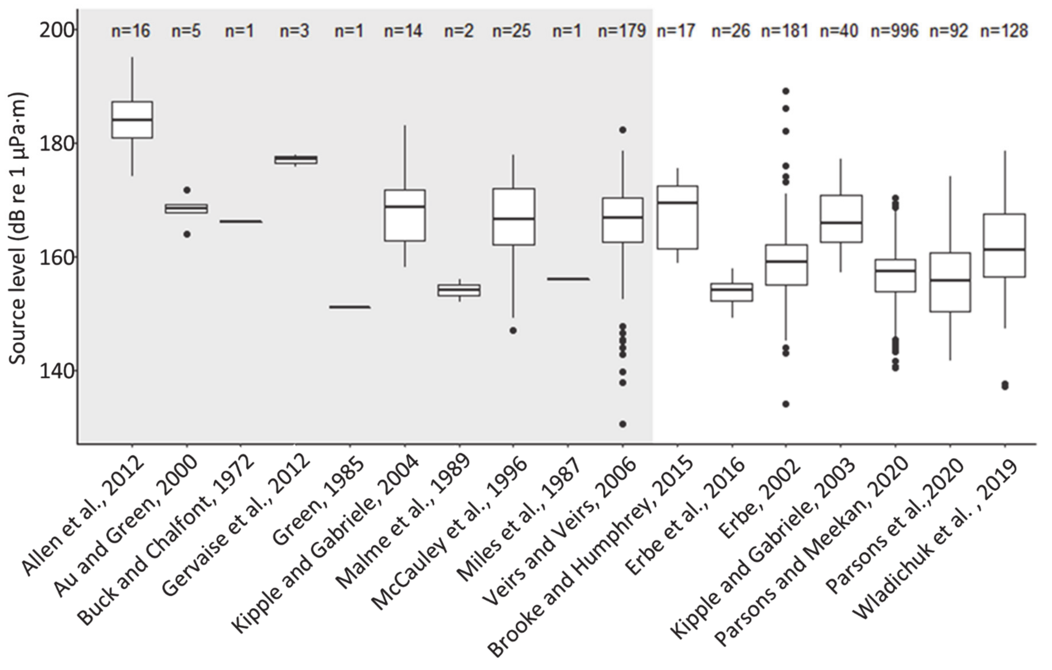
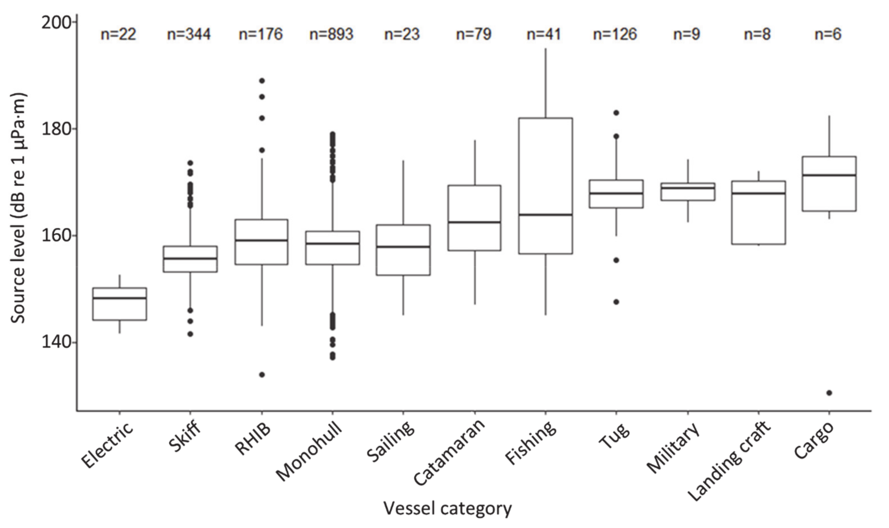
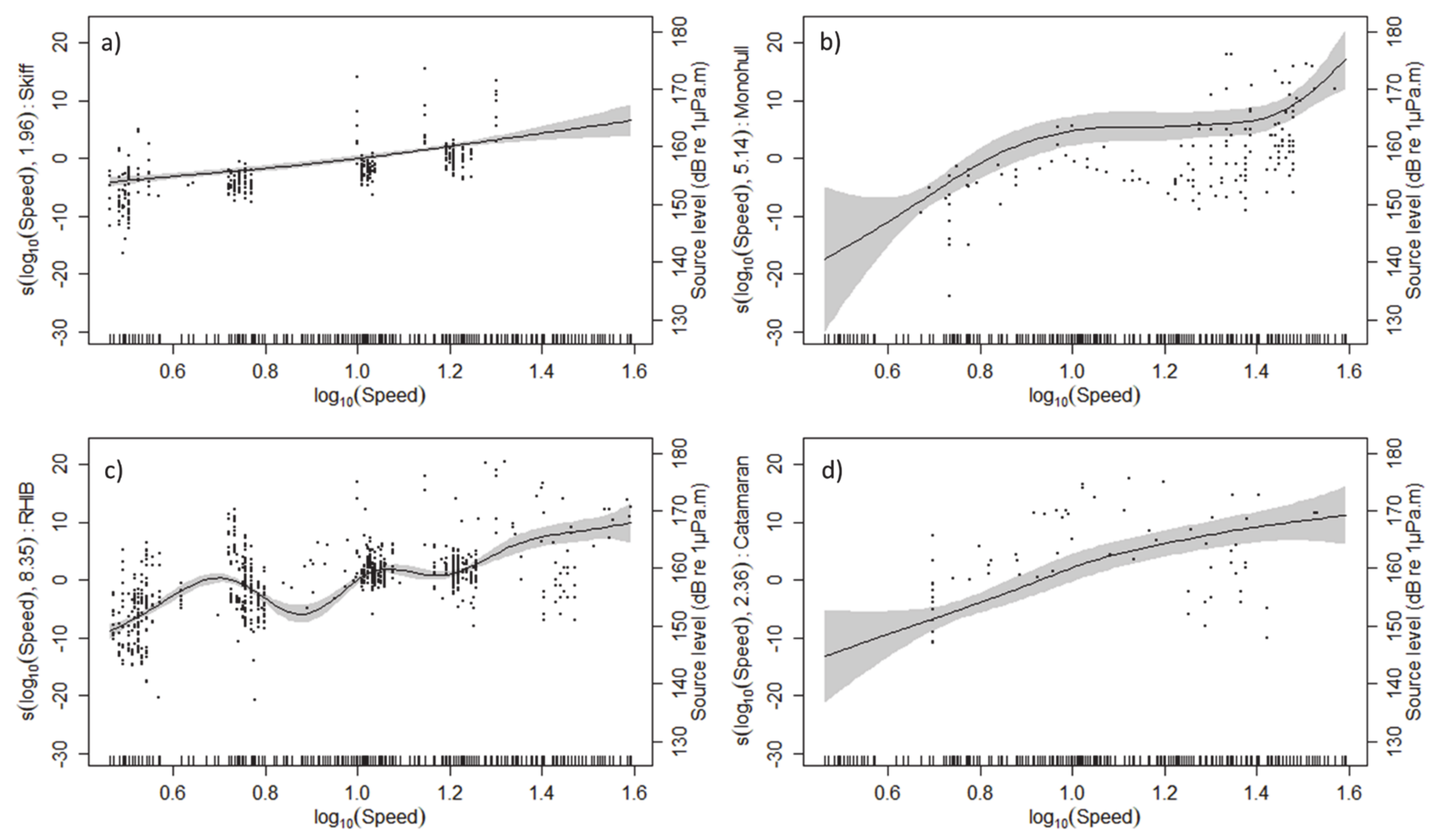
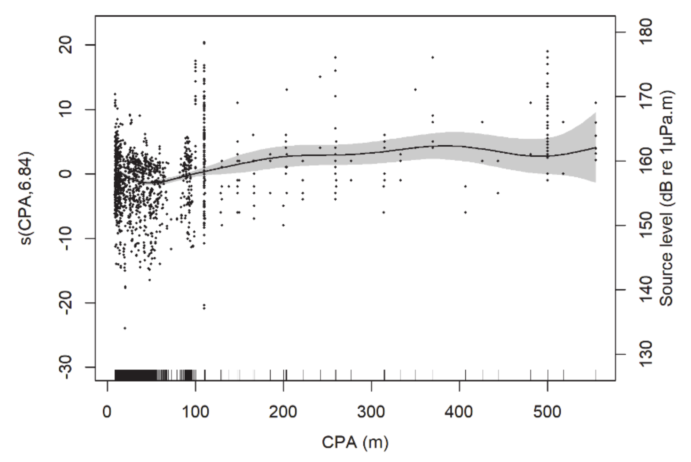
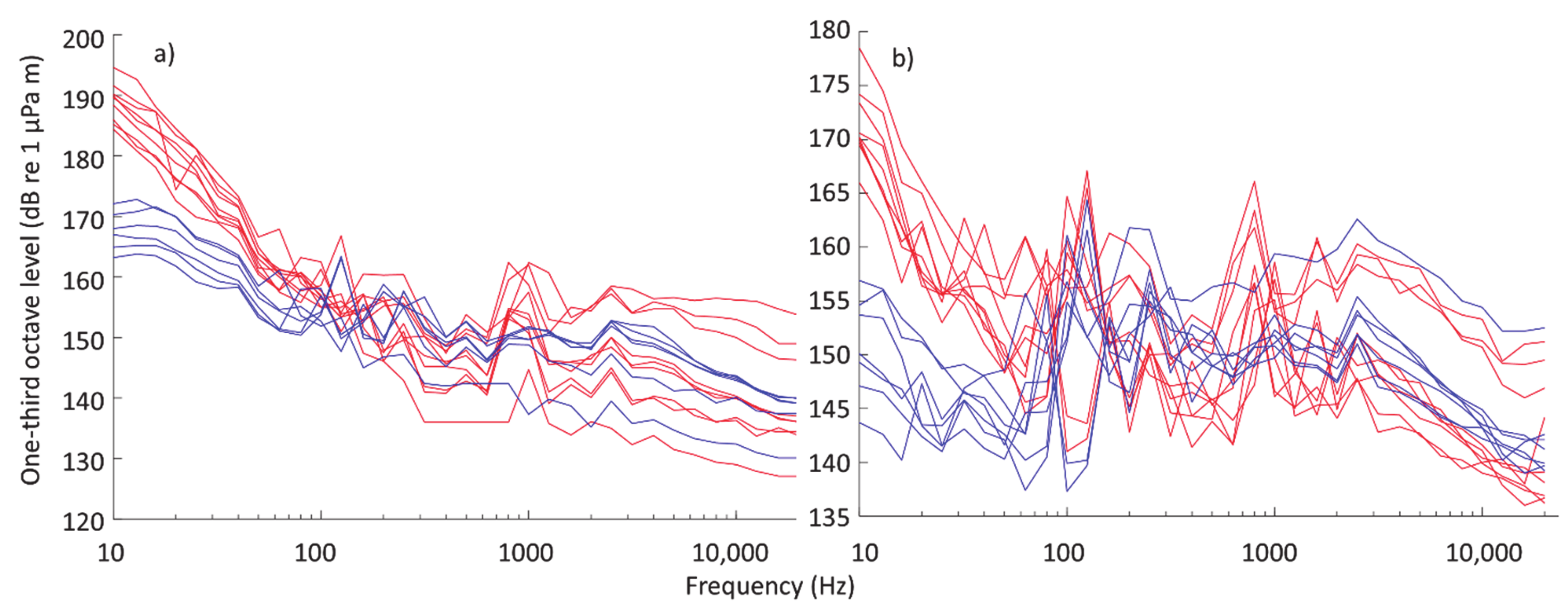
Table 1.
Categories of small vessels and their descriptions included in the study.
| Vessel Category | Vessel Type | Description | Hull Type | Lengths in Dataset (m) |
|---|---|---|---|---|
| 1 | Skiff | Single person or small crew, flat bottom, a pointed bow, and a square stern with tiller steering. Typically <10 m length | Planing | 4.3–10 |
| 2 | RHIB | Rigid hull inflatable boat. Typically, centre console, occasionally stern tiller <10 m length | Planing | 5–9.5 |
| 3 | Monohull | Single hull craft without further categorisation. Changes from displacement to planing condition as speed increases. Speed at which change between ploughing and planing occurs is vessel specific. | Semi- displacement | 3.4–24 |
| 4 | Tug | Small, powerful vessel designed particularly to tow or push barges and large ships. | Displacement | 15–25 |
| 5 | Landing craft | Any naval craft designed for conveying troops and equipment from a transport to a beach in an amphibious assault. Typically includes flattened front. | Displacement | 6.4–7.9 |
| 6 | Catamaran | Equivalent of a monohull vessels, but with two separated slender hulls | Semi- displacement | 8.2–25 |
| 7 | Fishing boat | Commercial vessel designed with sufficient power to trawl or pull nets. Changes from displacement to planing hull as speed increases. Speed at which change between ploughing and planing occurs is vessel specific. | Semi- displacement | 10.4–25 |
| 8 | Sailing boat | Monohulled vessel | Displacement | 9–19.8 |
| 9 | Electric | Any vessel powered by an electric motor, often limited in speed. Data recorded at ploughing speeds. | Displacement | 10 |
| 10 | Cargo | Monohull vessel used to transfer cargo. No further information provided. | Displacement | 24–25 |
| 11 | Military | Monohull vessel used for naval procedures. No further information provided. | Displacement | 22 |
Table 2.
Factors contributing to variations in source level and justifications for consideration in modelling in this study.
Table 2.
Factors contributing to variations in source level and justifications for consideration in modelling in this study.
| Factor | Justification | Example Citation | Considered | |
|---|---|---|---|---|
| Intrinsic characteristics | ||||
| Vessel type | Vessels designs are task-specific, thus type can impact acoustic signature | [21] | Yes | |
| Hull type | Affects the amount of water displaced and therefore the power required to propel the vessel | [38] | Yes | |
| Vessel length | Larger vessels require additional power (and thus noise) to move through water | [22] | Yes | |
| Beam | [3] | No | ||
| Engine power | Larger powered engines are associated with increased noise levels | [19] | Yes | |
| Engine type | Whether the engines are inboard or outboard may affect the position of the exhaust and noise radiated into the water | [19] | No | |
| Waterline angle | Angle of the hull to the waterline affects the propeller load and vessel drag, thus power and noise | [31] | No | |
| Draft | Affects the amount of water displaced by vessel and thus power required | [34] | No | |
| Propeller | Size | Propeller size, number of blades, gear ratio and propeller revolution rate dictate the frequency of acoustic tones | [22,38] | No |
| No. blades | No | |||
| Speed (rpm) | No | |||
| Gear ratio | No | |||
| Blade angle | No | |||
| Propeller (source) depth | Source depth affects signal propagation. However, in small vessels there is minimal difference in propeller depth between vessels | [31] | No | |
| Onboard machinery | Provides additional sources of noise. The number, size, power and condition of this machinery affects the noise emitted | [39,40] | No | |
| Speed | Source level shown to increase with increasing speed in large vessels | [22] | Yes | |
| Displacement | Increased load and resulting displacement requires additional power to attain the same speed | [34] | No | |
| Extrinsic factors | ||||
| Water depth | Water depth affects the propagation of an acoustic signal | [41] | Yes | |
| Closest point of approach (CPA) | The relationship between range and hydrophone depth can affect the Lloyd mirror pattern and therefore the received level and estimated noise levels | [19] | Yes | |
| Hydrophone depth | [19] | Yes | ||
| Type of propagation model applied | Whether a monopole or dipole source is considered and whether this is considered in the propagation model (RNL or MSL) affects the source estimate. | [19] | Yes | |
| Model source depth | Position of the source in the propagation model affects the received levels and may not always exactly reflect the actual propeller depth | [31] | No | |
| Hydrophone type and system frequency response | Sensitivity is often considered flat over all frequencies even though calibrations are often only conducted at a single frequency (typically 250 Hz). If frequency response is poor at low frequencies, energy is underestimated and thus so is the source level | [42] | No * | |
| Frequency band | If vessel energy is broadband and includes low-frequency energy, an increase in the lower frequency of the reported band can omit energy from the estimate | [43] | No † | |
| Environment conditions | Sea states/currents affect power required to achieve given speed and direction | [22] | No | |
* Although this information is often presented, details of frequency-dependent calibrations are often not given. † Frequency band is usually reported but has an interactive effect with type of propagation model used, hydrophone depth, water depth and CPA, and comprises two boundaries (high and low frequencies) as continuous variables and would have been complex to include in the statistical model.
Table 3.
Available variables and their measured or calculated units to include into the model, including available sample sizes and number of categorical levels gathered from published data (raw data only included), and sample sizes and number of categorical levels included in the final model.
Table 3.
Available variables and their measured or calculated units to include into the model, including available sample sizes and number of categorical levels gathered from published data (raw data only included), and sample sizes and number of categorical levels included in the final model.
| Variable | Data Type | Overall Sample Size (No. Levels) | Available No. Levels after Data Exploration |
|---|---|---|---|
| Vessel ID | Categorical | 1719 (224) | 49 |
| Vessel Type | Categorical | 1719 (11) | 4 |
| Hull Type | Categorical | 1719 (3) | 2 |
| Length | Continuous | 1719 | |
| Speed | Continuous | 1715 | |
| Engine Power | Continuous | 1519 | |
| Water depth | Continuous | 1714 | |
| Hydrophone depth | Continuous | 1714 | |
| Closest Point of Approach | Continuous | 1689 | |
| Propagation Model | Categorical | 1719 (3) | 3 |
| Reference | Categorical | 1719 (15) | 8 |
Table 4.
Details of the experimental designs and data processing of examined studies.
| Protocol | ||||||||||||
|---|---|---|---|---|---|---|---|---|---|---|---|---|
| Sample Size (n) | ||||||||||||
| From Reference Study | In Statistical Model | |||||||||||
| Article | Year | Location | Water Column (m) | Recordings | Vessels | Recordings | Vessels | Standard | CPA (km) | |||
| Allen et al. [58] | 2011 | Bar Harbour, ME, USA | 30–62 | 16 | 16 | 0 | 0 | x | 0.2–2.1 | |||
| Au and Green [59] | 1999 | Maui, HI, USA | 15–30 | 5 | 5 | 0 | 0 | x | 0.091 | |||
| Brooker and Humphrey [62] | 2014 | Tyneside, UK | 100 | 17 | 1 | 17 | 1 | x | 0.1 | |||
| Erbe [36] | 1999 | Haro Strait, BC, CAN and WA, USA | 70 | 181 | 17 | 157 | 14 | x | 0.01–1.85 | |||
| Erbe et al. [38] | 2016 | Cockburn Sound, WA, AUS | 8 | 26 | 1 | 26 | 1 | x | 0.008–0.018 | |||
| Gervaise et al. [60] | 2009 | Saguenay Fjord, QC, CAN | 170 | 3 | 3 | 0 | 3 | x | 0.214 | |||
| Kipple and Gabriele [61] | 2000, 2002 | Glacier Bay, AK, USA | 55–61 | 39 | 14 | 36 | 12 | x | 0.5 | |||
| Kipple and Gabriele [63] | 2003 | Glacier Bay, AK, USA. | 55 | 14 | 9 | 0 | 0 | x | 0.5 | |||
| McCauley et al. [34] | 1996 | Hervey Bay, QLD, AUS | 20 | 26 | 12 | 0 | 0 | x | Undefined | |||
| Parsons and Meekan [31] | 2019 | Lizard Island, QLD, AUS | 10 | 996 | 3 | 996 | 3 | x | 0.01–0.1 | |||
| Parsons et al. [52] | 2018 | Swan River, WA, AUS | 4 | 34 | 2 | 0 | 1 | x | 0.015–0.05 | |||
| Parsons et al. [52] * | 2018 | Swan River, WA, AUS | 4 | 58 | 51 | 0 | 0 | x | 0.015 | |||
| Wladichuk et al. [50,51] | 2017 | Haro Strait, BC, CAN and WA, USA | 200 | 128 | 25 | 111 | 15 | x | 0.11 | |||
| Veirs et al. [3] | 2011 | Haro Strait, BC, CAN and WA, USA | 70 | 179 | 66 | 0 | 0 | x | 1–3 | |||
| Total | 1727 | 230 | 1355 | 49 | ||||||||
| Hydrophones | ||||||||||||
| Article | Manufacturer | Hydrophone | No. Devices | Depth (m) | Sensitivity with Pre-Amp (dB re 1 V µPa−1) | Bandwidth Applied (kHz) | ||||||
| Allen et al. [58] | Cetacean Research | C54XRS | 3 | 5, 10, 25 | −20 | 0.001–2.5 | ||||||
| Au and Green [59] | Int. Trans. Corp. US Navy U.S.R.D. | TC-1032 and H-52 | 2 | 7.6 | Not given | 0.1–6 | ||||||
| Brooker and Humphrey [62] | Reson | TC4032 | 3 | 50 | −170 | 0.1–10 | ||||||
| Erbe [36] | International Transducer Corp. | TC-4123 | 1 | 5,10 | −145 | 0.01–22 | ||||||
| Erbe et al. [38] | High Tech, Inc. | 92WB | 1 | 8 | −160 | 0.01–40 | ||||||
| Gervaise et al. [60] | High Tech, Inc. | 96 MIN | 4 | 30–140 | −165 | 0.01–20 | ||||||
| Kipple and Gabriele [61] | Not given | Not given | 1 | 30, 50 | Not given | 0.01–35 | ||||||
| Kipple and Gabriele [63] | Not given | Not given | 1 | 30 | Not given | 0.01–35 | ||||||
| McCauley et al. [34] | Massa and Clevite | 1025-C and CH17 | 4 | 20 | −195 and −196 | 0.016–12.5 | ||||||
| Parsons and Meekan [31] | OceanInstruments | SoundTrap ST300 STD | 9 | 8.5 | −169 to −176 | 0.08–20 | ||||||
| Parsons et al. [52] | OceanInstruments | SoundTrap ST300 STD | 1 | 4 | −173.6 | 0.1–20 | ||||||
| Parsons et al. [52] * | OceanInstruments | SoundTrap ST300 STD | 1 | 4 | −173.6 | 0.1–20 | ||||||
| Wladichuk et al. [50,51] | Geospectrum Technologies Inc. | M36 | 2 | 197 | −165 ± 3 | 0.02–100 | ||||||
| Veirs et al. [3] | Reson | TC4032 | 1 | 10 | −164 | 0.012–40 | ||||||
| Data Processing | ||||||||||||
| Article | Propagation Loss * | Surface-Image Correction | Source Approximation | Source Depth | Source Level Type | Vessel Type Reported | ||||||
| Allen et al. [58] | HG | x | Dipole | x | RNL | 7 | ||||||
| Au and Green [59] | SG | x | Dipole | x | RNL | 2,3,6 | ||||||
| Brooker and Humphrey [62] | SG | x | Dipole | x | RNL | 6 | ||||||
| Erbe [36] | SG, RAMGeo, RAY | x✓✓ | Dipole | x | RNL and MSL | 2,3,6,8 | ||||||
| Erbe et al. [38] | SG, RAMGeo | x✓ | Dipole and Monopole | x | RNL and MSL | 2 | ||||||
| Gervaise et al. [60] | SG | x | Dipole | x | RNL | Undefined | ||||||
| Kipple and Gabriele [61] | SG | x | Dipole | x | RNL | 1,3,4,5,8 | ||||||
| Kipple and Gabriele [63] | SG | x | Dipole | x | RNL | 1,3,4,6,7 | ||||||
| McCauley et al. [34] | Linear regression | x | Dipole | x | RNL and ASL | 1,3,8,6 | ||||||
| Parsons and Meekan [31] | Linear regression | x | Dipole | x | RNL and ASL | 1,3 | ||||||
| Parsons et al. [52] | SG, RAMGeo | x✓ | Dipole and Monopole | ✓ | RNL and MSL | 3,9 | ||||||
| Parsons et al. [52] * | SG | x | Dipole | x | RNL | 1,2,3 | ||||||
| Wladichuk et al. [50,51] | SG and RAY | x✓ | Dipole and Monopole | x | RNL and MSL | 1,2,3,5,6,8 | ||||||
| Veirs et al. [3] | HG | x | Dipole | x | RNL | 1,2,3,4,7,10,11 | ||||||
* SG: Spherical Geometry, i.e., 20 log10(r). HG: Hybrid Geometry, i.e., [10.20] log10(r). RAMGeo: Range-dependent Acoustic Model. RAY: Ray tracing model. Linear regression: Least squares linear regression with a log function [31]. N.B. Insufficient information on the methods of Buck and Chalfont [54], Miles et al. [55], Malme et al. [56], and Greene [57] could be found for inclusion in Table 4. Upper panel: date and location where the recordings took place, height of the water column on deployment site, number of recordings taken, number of vessels recorded, number of vessels analysed in this study, whether or not observations were carried out using standard protocols, and the range of the closest points of approach (CPAs) of the vessels. Middle panel: hydrophones’ technical details, number of devices used, hydrophone deployment depth, and the bandwidth of the recordings reported. Bottom panel: backpropagation methods and corresponding source approximation and vessel types reported.
Table 5.
Results of the final GAMM. s() presents the details of the estimated smoother for each vessel type. Estimates for the intercept α and each smoothing term are given, as well as the standard error (SE), estimated degrees of freedom (edf), and approximate significance of the smooth terms as the t-value, F-statistics (F), and p-value. The variance and standard error (SE) are given for the random effects in the model.
| Parametric Terms | ||||||
|---|---|---|---|---|---|---|
| Fixed Effects | Estimate | SE | t-Value | edf | F | p-Value |
| Intercept α | 157.99 | 2.23 | 70.74 | <2 × 10⁻¹⁶ | ||
| s(CPA) | −2.78 | 2.65 | −1.05 | 6.84 | 13.41 | <2 × 10⁻¹⁶ |
| s(Speed)skiff | 2.76 | 0.79 | 3.47 | 1.96 | 89.4 | <2 × 10⁻¹⁶ |
| s(Speed)RHIB | 18.36 | 7.06 | 2.6 | 5.15 | 36.87 | <2 × 10⁻¹⁶ |
| s(Speed)monohull | 7.86 | 3.84 | 2.05 | 8.35 | 110.22 | <2 × 10⁻¹⁶ |
| s(Speed)catamaran | 5.58 | 3.35 | 1.67 | 2.36 | 28.57 | 4.58 × 10⁻¹⁴ |
| Random effects | Variance | SE | ||||
| Vessel ID | 15.09 | 3.89 | ||||
| Reference | 30.32 | 5.51 |
Publisher’s Note: MDPI stays neutral with regard to jurisdictional claims in published maps and institutional affiliations. |
© 2021 by the authors. Licensee MDPI, Basel, Switzerland. This article is an open access article distributed under the terms and conditions of the Creative Commons Attribution (CC BY) license (https://creativecommons.org/licenses/by/4.0/).
Share and Cite
MDPI and ACS Style
Parsons, M.J.G.; Erbe, C.; Meekan, M.G.; Parsons, S.K. A Review and Meta-Analysis of Underwater Noise Radiated by Small (<25 m Length) Vessels. J. Mar. Sci. Eng. 2021, 9, 827. https://doi.org/10.3390/jmse9080827
AMA Style
Parsons MJG, Erbe C, Meekan MG, Parsons SK. A Review and Meta-Analysis of Underwater Noise Radiated by Small (<25 m Length) Vessels. Journal of Marine Science and Engineering. 2021; 9(8):827. https://doi.org/10.3390/jmse9080827
Chicago/Turabian StyleParsons, Miles J. G., Christine Erbe, Mark G. Meekan, and Sylvia K. Parsons. 2021. "A Review and Meta-Analysis of Underwater Noise Radiated by Small (<25 m Length) Vessels" Journal of Marine Science and Engineering 9, no. 8: 827. https://doi.org/10.3390/jmse9080827
Note that from the first issue of 2016, this journal uses article numbers instead of page numbers. See further details here.