
Observer-Based Autopilot Heading Finite-Time Control Design for Intelligent Ship with Prescribed Performance


1
Navigation College, Dalian Maritime University, Dalian 116026, China
2
School of Automation Engineering, University of Electronic Science and Technology of China, Chengdu 611731, China
*
Author to whom correspondence should be addressed.
†
These authors contributed equally to this work.
J. Mar. Sci. Eng. 2021, 9(8), 828; https://doi.org/10.3390/jmse9080828
Submission received: 21 May 2021
/
Revised: 23 July 2021
/
Accepted: 24 July 2021
/
Published: 30 July 2021
(This article belongs to the Special Issue Manoeuvring and Control of Ships and Other Marine Vehicles)
Abstract
:Traffic engineering control is a major challenge in marine transportation. Cost efficiency and high performance demand advanced technologies for the ship control systems. This paper develops an autopilot heading control scheme based on a fuzzy state observer for an intelligent ship on this subject to track the prescribed function while calling for performance limitation and order execution time. A fuzzy logic system (FLS) is adopted to approximate the unknown uncertainties caused by the changes in water depth, wind, wave, ship loading, and speed in navigation. State observer is required to obtain unknown yaw rate. By adopting performance function and tracking error transformation techniques, the heading tracking error can converge to prescribed performance bounds. Taking settling time into account, the finite-time adaptive prescribed performance control algorithm can save more resources effectively. Based on the Lyapunov stability theory, the observer-based adaptive fuzzy control approach does not cause any unbounded signal, the system remains stable. Meanwhile, the autopilot heading control system with an unknown yaw rate and constraint state can benefit from the given design.
1. Introduction
As an important carrier or mode of transportation by sea, ships play an important role in global trade. Proper ship maneuvering is vitally important to the safety of ships, lives, and the environment. As is well known, human factors are one of main causes for marine accidents. Thus, to enhance the safety of navigation, the automation control of ship motion [1,2,3,4,5,6,7] has attracted more and more attention. The ship course is the most common way to change and control the ship’s motion attitude, especially when sailing in open waters. Therefore, research into course control has become an important branch of ship motion control study. Unfortunately, ship course control suffers from unknown parameters, functional uncertainties, and external disturbances. The mathematical model of ship course is widely affected by many factors, such as ship type and size, loading conditions, etc., which makes it difficult to accurately acquire prior knowledge of model. In addition, ship motion is persistently influenced by exogenous disturbances, such as wind, wave, and current. The noise and error existing in state measurement may also degrade control performance. Even under some situations, it is impossible to obtain necessary state information due to the breakdown of corresponding instruments. Thus, it is challenging to design a practical ship course control scheme.
In practical industrial applications, it may be not easy to directly measure the states in a timely manner, so many solutions are employed to solve the problem, such as input driven filter and observer. Among them, the observer is one of the common and powerful methods to deal with the above problems. Its broad applications generate a great deal of scientific and practical research, linear observer [8], high gain observer [9], the linear dynamic compensator [10], the full state observer [11], the passive state observer [12], and so on. Moreover, model uncertainties are also a pervasive problem in most engineering fields. Based on universal approximation theorem [13], fuzzy logic system [4], or NN (Neural Network) control [5] has been widely used to solve the control issues for nonlinear uncertain systems, and some significant results have been published in [14,15,16,17,18]. In reference [14], for an input–output linearization applied in nonlinear vessel steering system, the system was divided into a system with linear dynamics and a system with internal dynamics.
Especially when navigating in narrow channel with limited available depth, ship course control has high requirements for rapid response, which makes it of high practical value to achieve the expected value in a limited time, and a special type of prescribed performance is required, and the estimation error converges to a bounded set to ensure navigational safety. The convergence rate is an important performance index in the ship course control field. So far, most existing control schemes for ship course control guarantee asymptotic stability, which means that the coordination can only be achieved as time tends to infinity. Designing a control law that guarantees tracking performance with faster convergence is still an open issue. The basic idea of finite-time control is to achieve the fastest convergence speed of a closed-loop system in exponential form and ensure the stability of the control system at the same time [19,20,21]. By using finite-time stability criterion, finite-time stabilization control issue has been studied for rigid spacecraft in [22], and adaptive finite-time stabilization scheme has been developed for a strict feedback nonlinear system in [23]. State constraints are also an important issue that should be considered in ship course control. Many methods have been designed to handle the state constraint problem, for example, in [24], the problem of the tracking control with a prescribed performance bound for the marine surface vessels was solved. In [6], the constrained tracking control of the marine surface vessel was transformed into the stabilization of an unconstrained system. The authors of [19,20,21] investigated the adaptive fuzzy or NN finite-time control issues for nonlinear systems. To the authors’ knowledge, the problem of observer-based autopilot course tracking control for the intelligent ship with state constraint has not been studied in the existing literature, which is an interesting issue to be solved.
This paper focuses on the problem of observer-based adaptive fuzzy autopilot course performance constraint finite-time control. A state observer is constructed to estimate the unknown yaw rate state, and error transformation techniques are used to obtain the unconstrained state. The finite-time Lyapunov function is the basic theory of controller design and stability analysis. Compared with the existing works, the major contributions of this paper can be summarized as follows.
(1) This paper developed an observer-based adaptive fuzzy autopilot course finite-time control scheme for ship control systems. A fuzzy state observer is designed to lessen the needed information and design the controller of ship autopilot.
(2) Based on the performance function and tracking error transformation techniques, an autopilot course tracking error constraint control scheme is developed, which can ensure the course tracking error converges to a prescribed performance bound in finite-time.
2. Problem Formulation
2.1. Description of Autopilot Heading Control
In this paper, a ship heading control model is considered. Although it is a simple second-order response model, it includes all facts of ship autopilot system. Thus, it does matter to research such a typical model. According to literature [25], the following model can be given
where is rudder angle, is ship heading angle, and and stand for control input order and output information of ship autopilot, respectively. K denotes rudder gain, and T represents time constant, which can be obtained from experiment data. represents the internal unknown dynamic of system.
For the sake of facilitating above description in the state space form, we define , , and ; then, model (1) can be rewritten as
where is assumed to be unmeasurable. Obviously, is also an unknown smooth nonlinear function, which satisfies the Lipschitz condition, there is a known constant l such that , where is the estimation of .
Assumption 1.
For any , the reference ship heading signal and its time derivatives and satisfy , , , where , , and are the positive constants.
The control objective of this paper will be to design an observer-based adaptive fuzzy autopilot heading finite-time controller, such that the ship heading can track the given reference signal function in finite-time, and the heading tracking error can converge to a prescribed performance bound.
2.2. Prescribed Performance
Definition 1.
The prescribed performance can be described by the following inequality [26,27]:
where , , , a, are positive design parameters, . Consider the limited min and max is selected such that , . It follows from (3) that is guaranteed to be less than , and the performance bounds of the error can be determined by appropriately choosing the performance function and the parameters ,.
Remark 1.
is the performance state to be prescribed, inequality (4) prevents the prescribed error state from reaching the bounds . Note that the constrained error state can be either autopilot physical constraint or ship safety performance requirement.
2.3. Fuzzy Logic Systems
Lemma 1
([13]). Let be a continuous function defined over a compact set Ω. Then for any constant , there exists a FLS such that
where is the ideal weight vector. This paper assumes that is unknown and bounded, satisfies with a positive constant , ε is the fuzzy minimum approximation error, and there exists a positive constant that satisfies . is the fuzzy rules number, is fuzzy basic function vector with the property , is selected as Gaussian function such that
where and are the centers vector and width of Gaussian function, respectively.
2.4. Finite-Time Stability
To address the issue of finite-time control, the following Definition and Lemma will be given.
Definition 2
Lemma 2
([21]). There exists a positive definite function , with constants , , and , the nonlinear system satisfies
Then the nonlinear system is SGPFS.
3. Autopilot Control Design and Stability Analysis
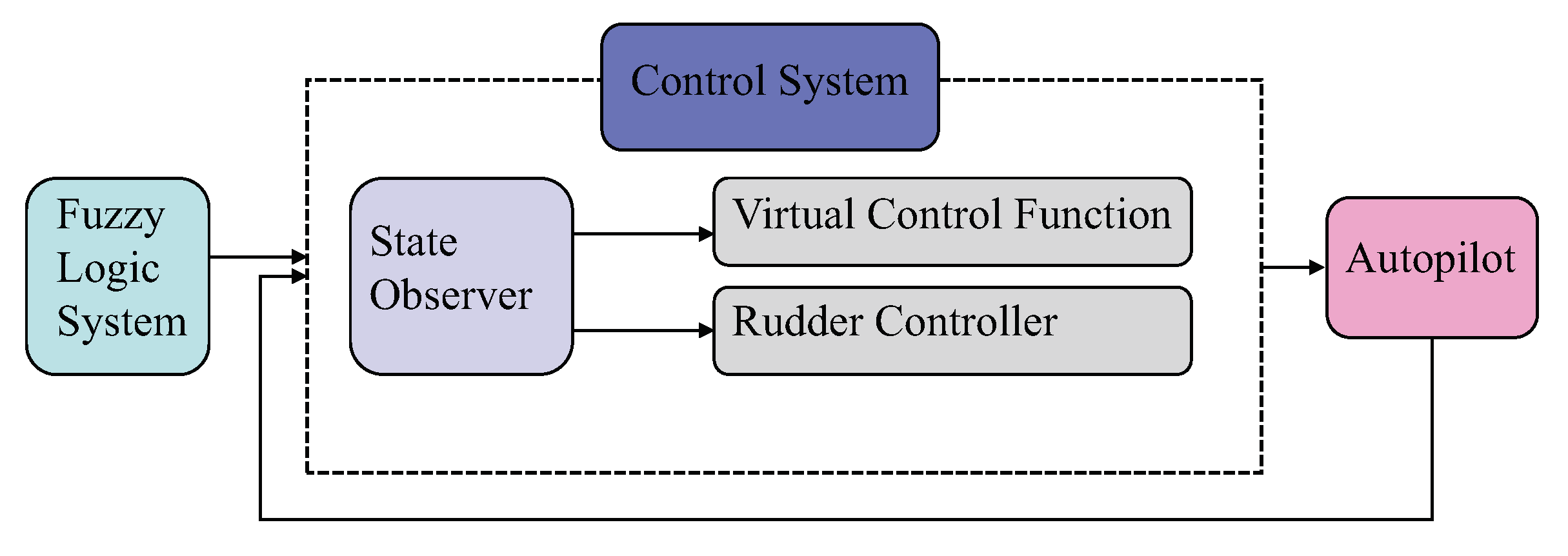
As shown in Figure 1, based on the Lyapunov function, observer-based finite-time autopilot heading control strategy and stability analysis are given in this section to ensure that the error constraint is not violated.
3.1. Adaptive Fuzzy State Observer Design
In practice, the yaw rate signal in the intelligent ship may not be available in many cases, and the state observer must be introduced to estimate the yaw rate information. In this section, the only available signal of plant (2) is y = , and the state observer serves to estimate the unknown yaw rate.
The adaptive fuzzy state observer is designed as
where and are observer gains, is the estimation of , is the estimation of , and is the estimation of .
Remark 2.
An adaptive fuzzy state observer is designed to deal with the problem of unmeasured states. Autopilot heading tracking control problems have been widely studied in [10,11]. However, in practical environments, due to the influence of water depth, wind, and waves, the ship’s heading and yaw rate of autopilot are not be measured directly, which inspired us to study the observer-based output feedback autopilot heading tracking control problems.
Rewritten (6) as
where , , , , .
We choose a vector M to make A be strict Hurwitz. Thus, given a matrix , there exists a matrix such that
Now, by adding and subtracting on the right side of the second subsystem in (2) and using (4), system (2) can be transformed as
where .
Since is an unknown function, from Lemma 1, in (9) can be approximated by the FLS and assume that
where is the approximate error.
Define the observe errors vector as . According to (4), (7), and (9), the dynamics of the observe errors can be obtained
where , , is the estimation error.
Choose the Lyapunov function candidate , the time derivative of is
Applying Young’s inequality yields
Substituting (13)–(15) into (12) results in
where , .
3.2. Design and Stability Analysis of Autopilot Heading Tracking Control
When designing a high-performance controller, the improvement of transient response is a crucial object that must be addressed. Taking settling time into account, define finite-time virtual control and rudder angle u to control heading angle y, that is to say, the task is to have a fast convergence rate with unknown yaw rate and constraint error in a settling time. Firstly, transfer the coordinate as
where is the virtual error surface, r is a state variable, is the intermediate control function, and is the error between r and . To achieve the performance constraint problem, one can transform the constrained tracking error behavior into an equivalent unconstrained state. Consider the following equation
where is the transformed error and is a smooth, strictly increasing function; then, one can obtain , from the definition of and (18), and one can get
where , defining the following state transformation as
Then, one can get
Inspired by [24], one can obtain that if is bounded, then the prescribed performance as shown in (17) of is satisfied. The backstepping controller of ship autopilot is defined as follows.
Step 1: According to (6), (17) and , the time derivative of is
The candidate Lyapunov function is chosen as
It follows from (9), (16), (17), (23), and (24), that the time derivative of satisfies
Applying Young’s inequality yields
Substituting (26) into (25) yields
where .
The intermediate control function is
where is a design parameter.
Substituting (28) into (27) yields
Define the following first-order filter to avoid repeatedly differentiating :
where is a design parameter.
It follows from (17) that
where is a continuous nonlinear function.
Step 2: From (6) and (17), one has
Consider the Lyapunov function V as
where is a design parameter.
Along with the solution of (17), (23), (29), (32), and (33), the derivative of V can be expressed as
Applying Young’s inequality again yields
and substituting (35) into (34) yields
The the actual controller u and the parameter adaptive law of is
where and are design parameters.
4. Stability Analysis
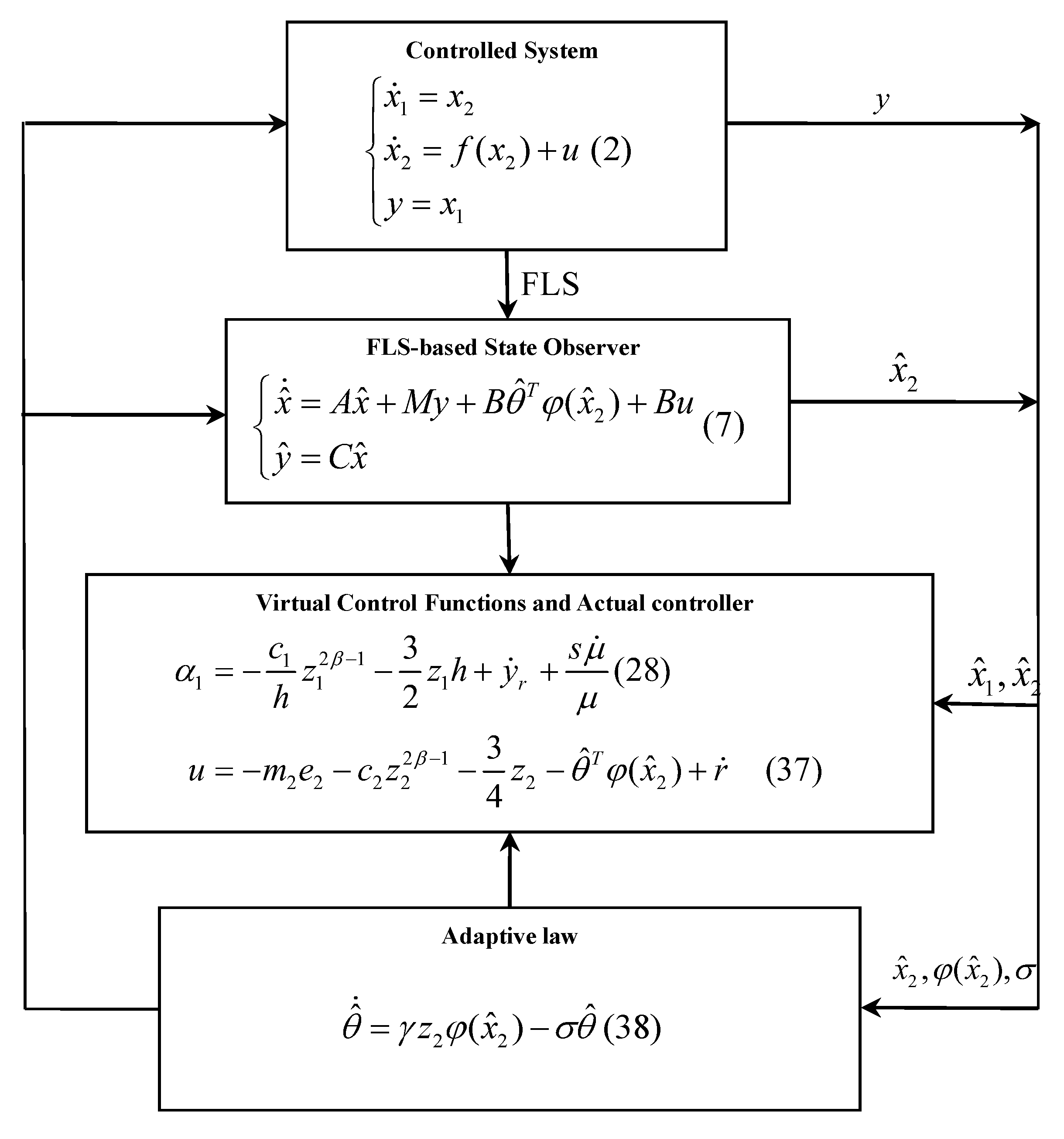
The property of the developed observer-based autopilot heading finite-time control scheme via performance constraint can be summarized as following theorem. Therefore, the graph of the above control scheme is shown in Figure 2.
Theorem 1.
Consider the autopilot heading control system (1), under Definitions 1 and 2, Assumption 1, and Lemmas 1 and 2, and based on the designed state observer (6), control rudder (37), and parameter adaptive law (38), one can ensure that all signals in the closed-loop system are bounded and that the error constraint is not violated.
Proof.
Choose the whole Lyapunov function as
From (16), (33), and (34), by substituting (37) and (38) into (36), the time derivative of V is
Using Young’s inequality, one has
where with positive constant . □
Substituting (40) and (41) into (39) yields
where , .
Assume that , and for a given , all initial conditions satisfy . According to Assumption 1, for any and d, the sets and are compacts in and R, respectively, and thus, set is also compact in . Then, (42) can be rewritten as
Define , one has
According to [27], the following expression holds
where and are constant, is a real-valued function, which yields
By substituting (33), (46), and (47) into (44), using inequality from [28], one has
where and .
From Lemma 3 and the proof in [27,29], for any constant , one has
where initial values , , and . From the definition of (), when , one has , , and , thus, the controlled system is SGPFS.
From (48), it can be shown that , , , , e, , and are bounded. From (3), one can obtain that , where and are design parameters. Moreover, according to [28], one can make the observer, tracking and estimation errors to be small by suitable design parameters , , , , , , and . Therefore, the design parameters should be selected properly for achieving the desired transient performance and control objective. This completes the proof of Theorem 1.
5. Simulation Study
In this section, simulation results are given to explain the feasibility of the developed control algorithm and theory.
The ship autopilot parameters can be selected in [25] with the ship particulars as follows: forward speed 7.72 m/s, block coefficient 0.681, draft 8 m, breath molded , length between perpendiculars . From the above ship particulars, choose the autopilot model parameters as , , , .
The desired heading signal is given by a representative practical mode as
where is an order heading signal, is the desired autopilot performance for ship heading during the ship heading control:
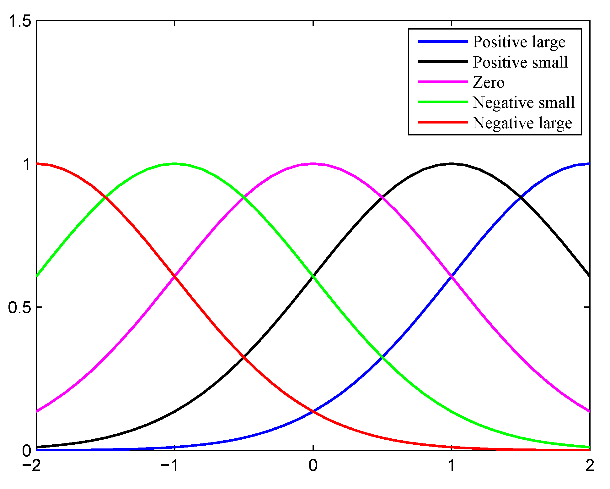
In this simulation, the five fuzzy sets: are selected over the intervals . The following fuzzy IF-THEN rules are chosen as
Select the fuzzy sets as follows: , , , , , , , , , . is negative large, is negative small, is zero, is positive small, and is the positive large. Choose the membership functions (displayed by Figure 3) as
In simulation, the design parameters in controller and adaptive law are selected as , , , , .
The initial conditions of variables and parameters are selected as: , , , , .
The performance function can be selected as
where , , .
Choose the observer gains as and , positive definite matrix , thus, by solving the Lyapunov Equation (9), we have positive definite matrix P as .
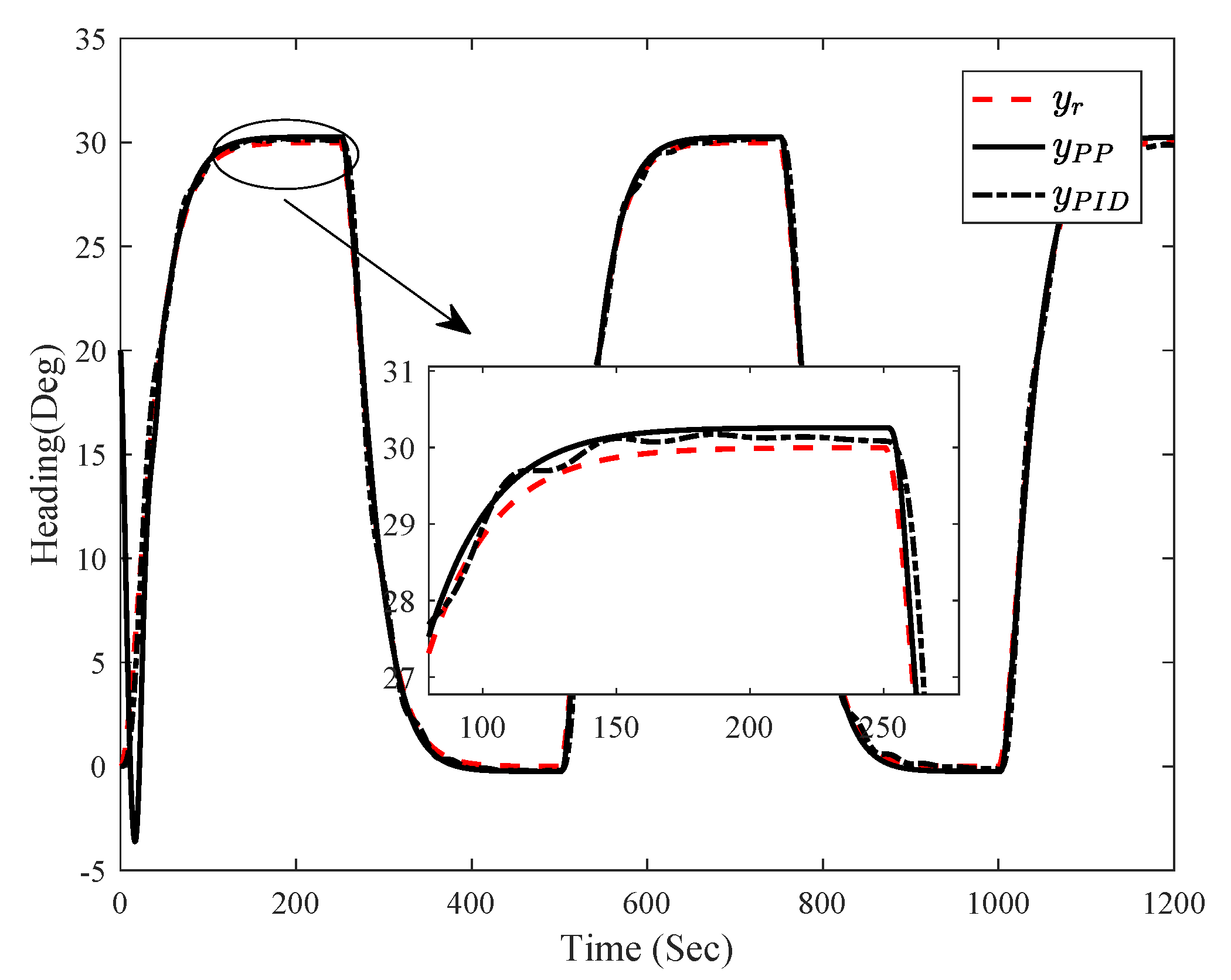
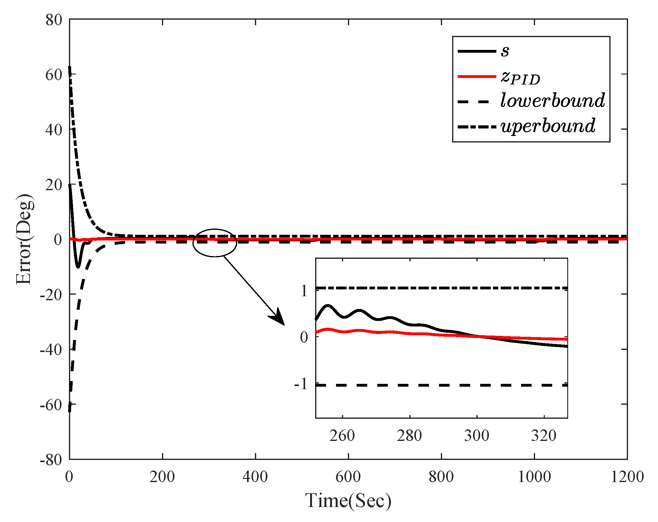
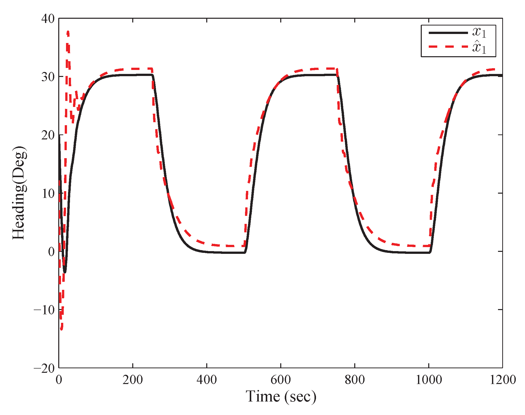
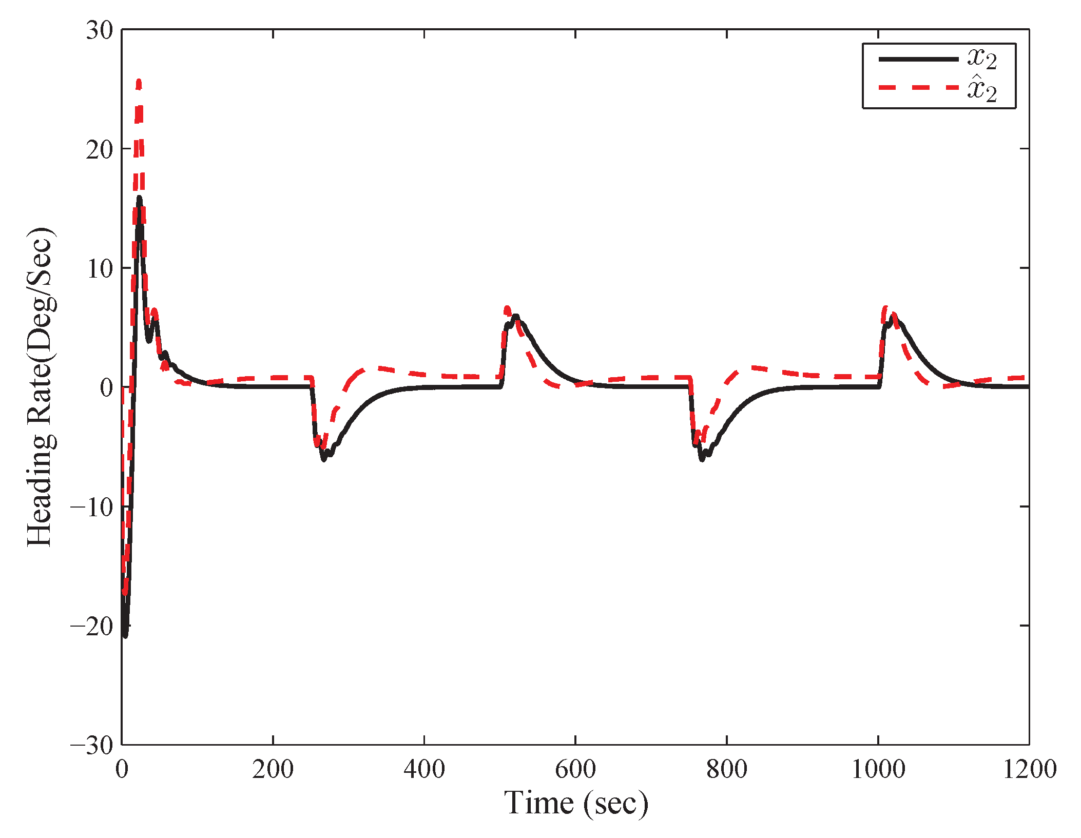
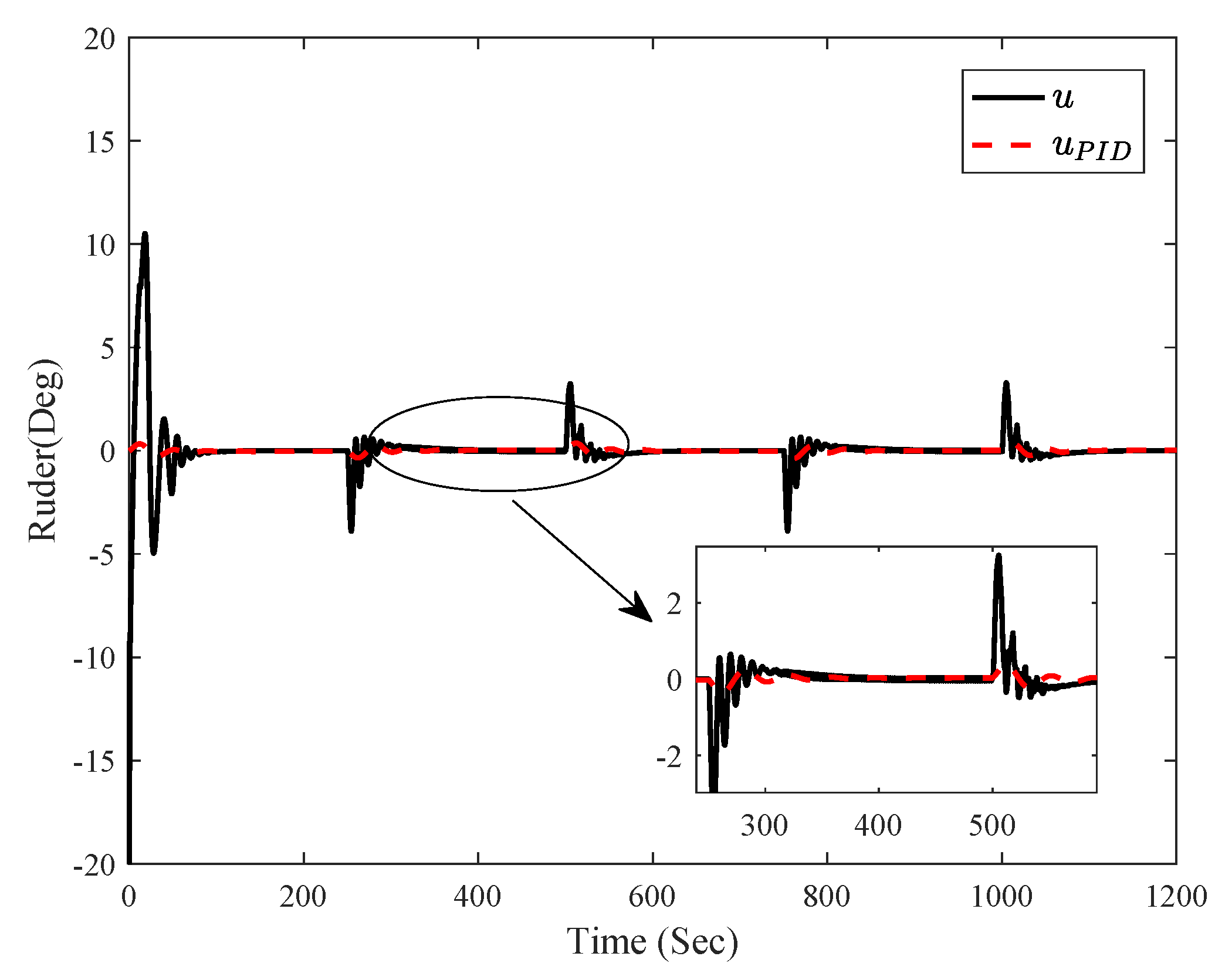
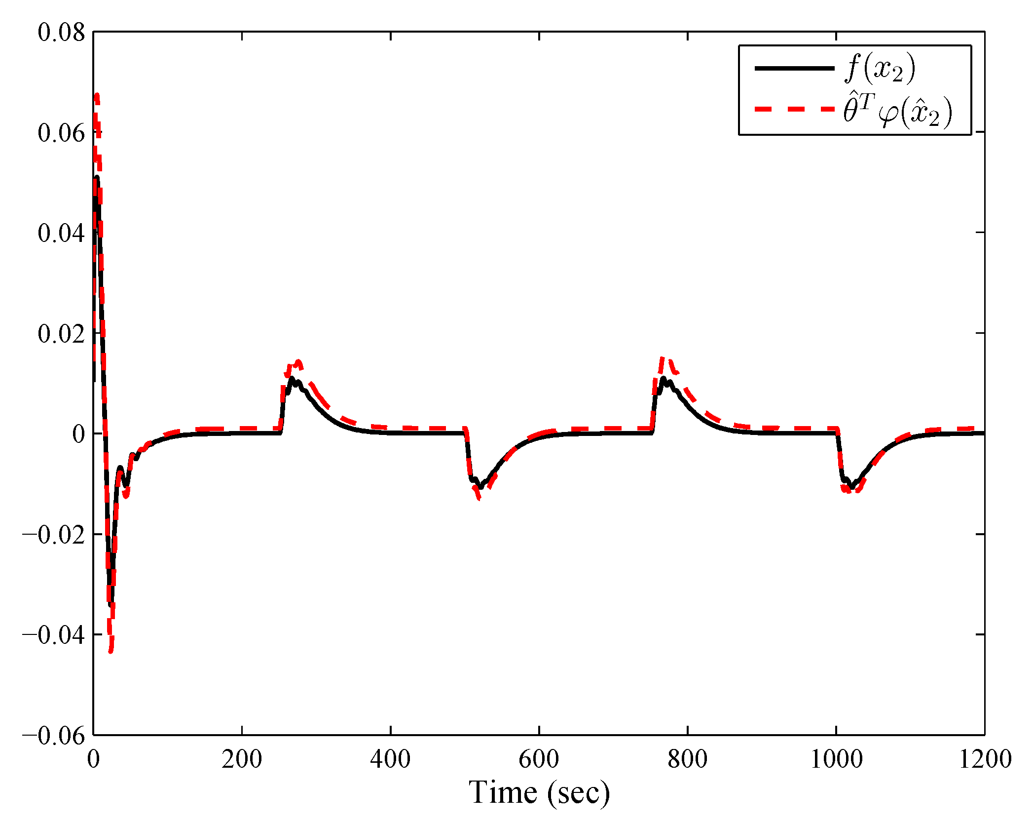
The simulation results are displayed by Figure 4, Figure 5, Figure 6, Figure 7, Figure 8, Figure 9 and Figure 10, where Figure 4 compares trajectories of ship’s heading and its desired heading angle; Figure 5 shows the comparing tracking error curve with PID method; Figure 6 and Figure 7 show the ship’s heading, yaw rate and their estimations, respectively; Figure 8 shows the comparing rudder angle curve with PID method; and Figure 9 show the curves of FLS and function .
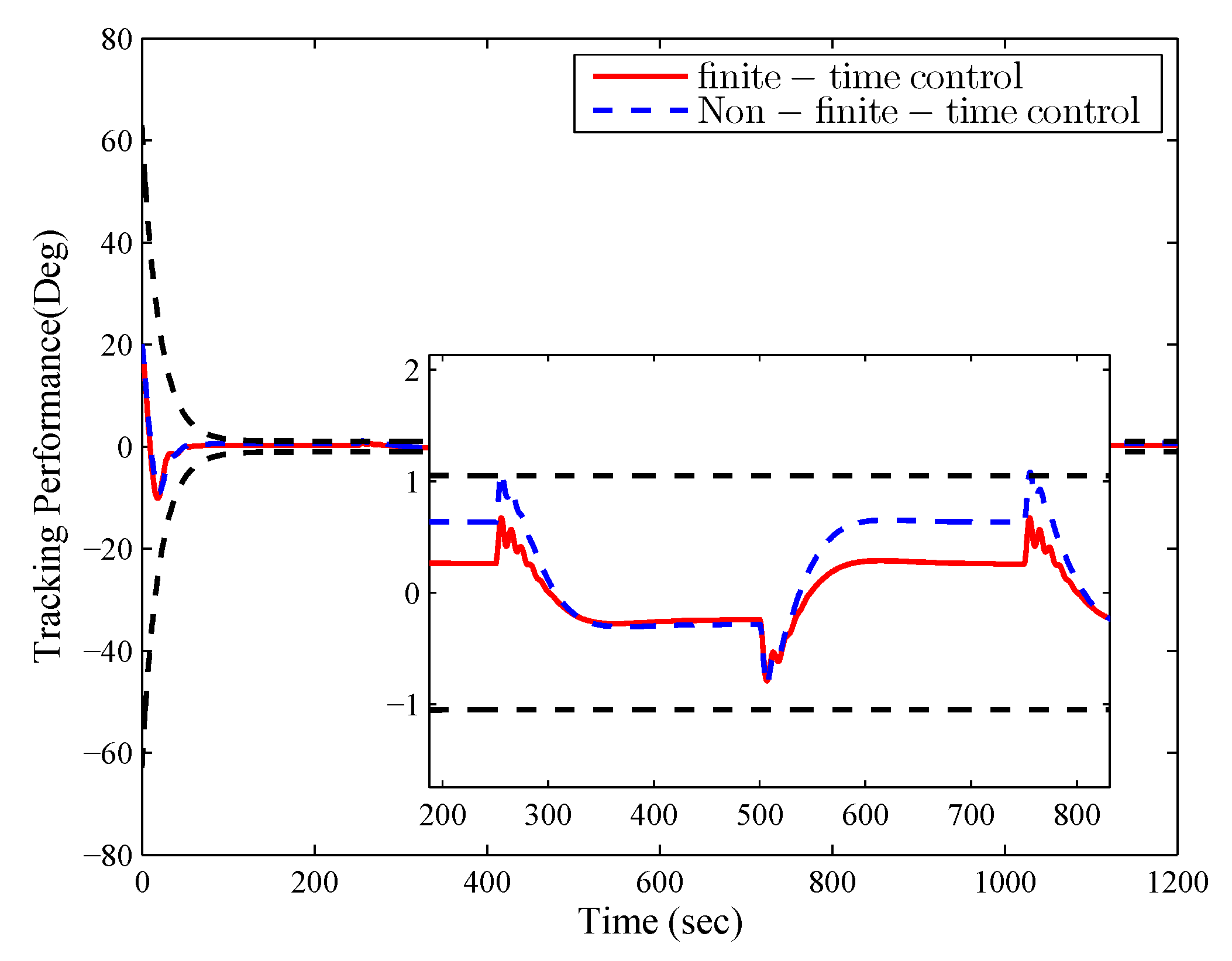
It can be see from Figure 10 that the developed autopilot heading tracking control can guarantee the tracking error converges to a prescribed performance bound, and finite-time control has a better performance. As shown in Figure 6 and Figure 7, the designed fuzzy state observer solves the problem of unmeasured states. Thus, the effectiveness of the developed control method can be verified.
Remark 3.
Since the finite-time controller contains the term of exponential power, thus, finite-time control has high precision performance and fast transient performances. To explain the effectiveness of the developed control scheme, we make the following comparison. Note that the control performance of the developed finite-time control are mainly influenced by the parameter β; we choose the same design parameters, initial values, and fuzzy membership functions except β, if , which belong to non-finite-time control. The comparison result is displayed by Figure 10.
6. Conclusions
In this paper, we have investigated the observer-based autopilot heading adaptive fuzzy control problem for intelligent ship with prescribed performance. A fuzzy state observer was first established to obtain the unknown yaw rate. By combining backstepping recursive design with the DSC technique, the stability of the intelligent ship autopilot system has been given utilizing the finite-time Lyapunov stability theory. The developed control algorithm has not only solved the adaptive fuzzy autopilot heading tracking control but also guarantees the tracking error converges to a prescribed performance bound in finite-time. The future research direction will focus on observer-based robust adaptive fuzzy autopilot heading fault-tolerant control for intelligent ship autopilot system with full-state constraint, parameter, or input uncertainties.
Although some progress has been achieved, there are still some other challenges in the field, for instance, robust position control [30], station-keeping control [31], robust control [32], neuro-fuzzy system [29], a simplified computer dynamics model [33], fuzzy sliding mode control [34], etc., which will be our future research direction.
Author Contributions
Conceptualization, L.Z. and T.L.; methodology, L.Z.; software, L.Z.; validation, L.Z. and T.L.; formal analysis, L.Z.; investigation, L.Z.; resources, T.L.; data curation, L.Z.; writing—original draft preparation, L.Z.; writing—review and editing, T.L.; visualization, L.Z.; supervision, T.L.; project administration, T.L.; funding acquisition, T.L. All authors have read and agreed to the published version of the manuscript.
Funding
This work is supported in part by the National Natural Science Foundation of China (under Grant Nos. 51939001, 61976033); the Science and Technology Innovation Funds of Dalian (under Grant No. 2018J11CY022); the Liaoning Revitalization Talents Program (under Grant Nos. XLYC1908018); the Natural Science Foundation of Liaoning (2019-ZD-0151); the Fundamental Research Funds for the Central Universities (under Grant No. 3132019345).
Institutional Review Board Statement
Not applicable.
Informed Consent Statement
Not applicable.
Data Availability Statement
Not applicable.
Conflicts of Interest
The authors declare no conflict of interest.
References
- Minorsky, N. Directional stability of automatically steered bodies. J. Am. Soc. Nav. Eng. 1992, 34, 280–309. [Google Scholar] [CrossRef]
- Kallstrom, C. Adaptive autopilots for tankers. Automatica 1979, 15, 241–254. [Google Scholar] [CrossRef]
- Yang, Y.S.; Zhou, C.J.; Ren, J.S. Model reference adaptive robust fuzzy control for ship steering autopilot with uncertain nonlinear systems. Appl. Soft Comput. 2003, 3, 305–316. [Google Scholar] [CrossRef]
- Yang, Y.S.; Ren, J.S. Adaptive fuzzy robust tracking controller design via small gain approach and its application. IEEE Trans. Fuzzy Syst. 2003, 11, 783–795. [Google Scholar] [CrossRef]
- Tung, L.T. Design a ship autopilot using neural network. J. Ship Prod. Des. 2017, 33, 192–196. [Google Scholar] [CrossRef]
- Dai, S.; Wang, M.; Wang, C. Neural learning control of marine surface vessels with guaranteed transient tracking performance. Ind. Electron. IEEE Trans 2016, 63, 1717–1727. [Google Scholar] [CrossRef]
- Perera, L.P.; Soares, C.G. Pre-filtered sliding mode control for nonlinear ship steering associated with disturbances. Ocean. Eng. 2012, 51, 49–62. [Google Scholar] [CrossRef]
- Zhou, Y.; Li, R.; Zhao, D.; Wu, Q. Ship course control using LESO with wave disturbance. In Proceedings of the IEEE International Conference on Robotics and Biomimetics, Qingdao, China, 3–7 December 2016. [Google Scholar]
- Du, J.; Hu, X.; Liu, H.; Chen, C. Adaptive robust output feedback control for a marine dynamic positioning system based on a high-gain observer. IEEE Trans. Neural Netw. Learn. Syst. 2015, 26, 2775–2786. [Google Scholar] [CrossRef]
- Wang, Z.W.; Peng, X.Y. Control of ship course based on NN-adaptive output feedback. Trans. Beijing Inst. Technol. 2011, 31, 425–429. [Google Scholar]
- Zheng, Y.F.; Li, J.M.; Li, R.H. Output feedback control design for ship’s course keeping nonlinear system based on state observer. In Proceedings of the 29th Chinese Control Conference, Beijing, China, 29–31 July 2010; pp. 606–609. [Google Scholar]
- Peng, X.Y.; Hu, Z.H. Adaptive nonlinear output feedback control with wave filter for ship course. Control. Theory Appl. 2013, 30, 863–868. [Google Scholar]
- Wang, L.X. Stable adaptive fuzzy control of nonlinear systems. IEEE Trans. Fuzzy Syst. 1993, 1, 146–155. [Google Scholar] [CrossRef]
- Perera, L.P.; Soares, C.G. Lyapunov and Hurwitz based controls for input–output linearisation applied to nonlinear vessel steering. Ocean. Eng. 2013, 66, 58–68. [Google Scholar] [CrossRef]
- Weng, Y.; Wang, N.; Soares, C.G. Data-driven sideslip observer-based adaptive sliding-mode path-following control of underactuated marine vessels. Ocean. Eng. 2020, 197, 106910. [Google Scholar] [CrossRef]
- Hx, A.; Tif, B.; Cgs, A. Uniformly semiglobally exponential stability of vector field guidance law and autopilot for path-following. Eur. J. Control. 2020, 53, 88–97. [Google Scholar]
- Wang, N.; Sun, Z.; Su, S.F.; Wang, Y.Y. Fuzzy uncertainty observer-based path-following control of underactuated marine vehicles with unmodeled dynamics and disturbances. Int. J. Fuzzy Syst. 2018, 20, 2593–2604. [Google Scholar] [CrossRef]
- Perera, L.P.; Carvalho, J.P.; Soares, C.G. Intelligent Ocean Navigation and Fuzzy-Bayesian Decision/Action Formulation. IEEE J. Ocean. Eng. 2012, 37, 204–219. [Google Scholar] [CrossRef]
- Wang, F.; Chen, B.; Liu, X.P.; Lin, C. Finite-time adaptive fuzzy tracking control design for nonlinear systems. IEEE Trans. Fuzzy Syst. 2018, 26, 1207–1216. [Google Scholar] [CrossRef]
- Sun, Y.M.; Lin, B.C.; Wang, H.H. Finite-time adaptive control for a class of nonlinear systems with nonstrict feedback structure. IEEE Trans. Cybern. 2018, 48, 2774–2782. [Google Scholar] [CrossRef]
- Wang, F.; Chen, B.; Lin, C.; Zhang, J.; Meng, X.Z. Adaptive neural network finite-time output feedback control of quantized nonlinear systems. IEEE Trans. Cybern. 2018, 48, 1839–1848. [Google Scholar] [CrossRef]
- Zhu, Z.; Xia, Y.Q.; Fu, M.Y. Attitude stabilization of rigid spacecraft with finite-time convergence. Int. J. Robust Nonlinear Control. 2011, 21, 686–702. [Google Scholar] [CrossRef]
- Khoo, S.Y.; Yin, J.L.; Man, Z.H.; Yu, X.H. Finite-time stabilization of stochastic nonlinear systems in strict-feedback form. Automatica 2013, 49, 1403–1410. [Google Scholar] [CrossRef]
- Si, W.; Dong, X. Neural prescribed performance control for uncertain marine surface vessels without accurate initial errors. Math. Probl. Eng. 2017, 2017, 2618323.1–2618323.11. [Google Scholar] [CrossRef]
- Li, T.S.; Wang, D.; Feng, G.; Tong, S.C. A DSC approach to robust adaptive NN tracking control for strict-feedback nonlinear systems. IEEE Trans. Syst. Man Cybern. Part B 2010, 40, 915–927. [Google Scholar]
- Bechlioulis, C.P.; Rovithakis, G.A. A low-complexity global approximation-free control scheme with prescribed performance for unknown pure feedback systems. Automatica 2014, 50, 1217–1226. [Google Scholar] [CrossRef]
- Qian, C.J.; Lin, W. Non-lipschitz continuous stabilizers for nonlinear systems with uncontrollable unstable linearization. Syst. Control. Lett. 2001, 42, 185–200. [Google Scholar] [CrossRef]
- Li, Y.M.; Li, K.W.; Tong, S.C. Adaptive neural network finite-time control for multi-input and multi-output nonlinear systems with positive powers of odd rational numbers. IEEE Trans. Neural Netw. Learn. Syst. 2020, 31, 2532–2543. [Google Scholar] [CrossRef]
- Nicolau, V. Neuro-fuzzy system for intelligent course control of underactuated conventional ships. In Proceedings of the IEEE International Workshop on Soft Computing Applications, Gyula, Hungary, 21–23 August 2007; pp. 95–101. [Google Scholar]
- Vu, M.T.; Le, T.-H.; Thanh, H.L.N.N.; Huynh, T.-T.; Van, M.; Hoang, Q.-D.; Do, T.D. Robust Position Control of an Over-actuated Underwater Vehicle under Model Uncertainties and Ocean Current Effects Using Dynamic Sliding Mode Surface and Optimal Allocation Control. Sensors 2021, 21, 747. [Google Scholar] [CrossRef] [PubMed]
- Vu, M.T.; Thanh, H.L.N.N.; Huynh, T.T.; Do, Q.T.; Do, T.D.; Hoang, Q.D.; Le, T.H. Station-Keeping Control of a Hovering Over-Actuated Autonomous Underwater Vehicle Under Ocean Current Effects and Model Uncertainties in Horizontal Plane. IEEE Access 2020, 9, 6855–6867. [Google Scholar] [CrossRef]
- Thanh, H.L.N.N.; Vu, M.T.; Mung, N.X.; Nguyen, N.P.; Phuong, N.T. Perturbation Observer-Based Robust Control Using a Multiple Sliding Surfaces for Nonlinear Systems with Influences of Matched and Unmatched Uncertainties. Mathematics 2020, 8, 1371. [Google Scholar] [CrossRef]
- Borkowski, P.; Zwierzewicz, Z. Ship course stabilization based on a simplified computer dynamics model. Sci. J. Marit. Univ. Szczec. 2005, 5, 97–109. [Google Scholar]
- Han, Y.Z.; Pan, H.R.X.W.; Wang, C. A fuzzy sliding mode controller and its application on ship course control. In Proceedings of the 7th International Conference on Fuzzy Systems and Knowledge Discovery, Yantai, China, 10–12 August 2010; pp. 635–638. [Google Scholar]
Figure 1.
The flowchart of the sequence of steps of the proposed method.

Figure 2.
The graph of the above control scheme.

Figure 3.
The membership functions.

Figure 4.
Curves of ship’s heading and its desired heading angle.

Figure 5.
Curves of tracking error and performance boundeds.

Figure 6.
Curves of ship’s heading and its estimation.

Figure 7.
Curves of ship’s heading rate and its estimation.

Figure 8.
Curves of controllers.

Figure 9.
Curves of nonlinear function and its estimation.

Figure 10.
Tacking errors of finite-time and non-finite-time controll methods.

Publisher’s Note: MDPI stays neutral with regard to jurisdictional claims in published maps and institutional affiliations. |
© 2021 by the authors. Licensee MDPI, Basel, Switzerland. This article is an open access article distributed under the terms and conditions of the Creative Commons Attribution (CC BY) license (https://creativecommons.org/licenses/by/4.0/).
Share and Cite
MDPI and ACS Style
Zhu, L.; Li, T. Observer-Based Autopilot Heading Finite-Time Control Design for Intelligent Ship with Prescribed Performance. J. Mar. Sci. Eng. 2021, 9, 828. https://doi.org/10.3390/jmse9080828
AMA Style
Zhu L, Li T. Observer-Based Autopilot Heading Finite-Time Control Design for Intelligent Ship with Prescribed Performance. Journal of Marine Science and Engineering. 2021; 9(8):828. https://doi.org/10.3390/jmse9080828
Chicago/Turabian StyleZhu, Liyan, and Tieshan Li. 2021. "Observer-Based Autopilot Heading Finite-Time Control Design for Intelligent Ship with Prescribed Performance" Journal of Marine Science and Engineering 9, no. 8: 828. https://doi.org/10.3390/jmse9080828
Note that from the first issue of 2016, this journal uses article numbers instead of page numbers. See further details here.