
Vine Identification and Characterization in Goblet-Trained Vineyards Using Remotely Sensed Images


1
Ecole Supérieure d’Ingénieurs d’Agronomie Méditerranéenne de l’Université Saint-Joseph de Beyrouth, Taanayel, Lebanon
2
Ecole Supérieure d’Ingénieurs de Beyrouth de l’Université Saint-Joseph de Beyrouth, Mar Roukoz, Lebanon
*
Author to whom correspondence should be addressed.
Remote Sens. 2021, 13(15), 2992; https://doi.org/10.3390/rs13152992
Submission received: 13 June 2021
/
Revised: 16 July 2021
/
Accepted: 20 July 2021
/
Published: 29 July 2021
(This article belongs to the Special Issue Remote Sensing Applications in Agricultural Ecosystems)
Abstract
:This paper proposes a novel approach for living and missing vine identification and vine characterization in goblet-trained vine plots using aerial images. Given the periodic structure of goblet vineyards, the RGB color coded parcel image is analyzed using proper processing techniques in order to determine the locations of living and missing vines. Vine characterization is achieved by implementing the marker-controlled watershed transform where the centers of the living vines serve as object markers. As a result, a precise mortality rate is calculated for each parcel. Moreover, all vines, even the overlapping ones, are fully recognized providing information about their size, shape, and green color intensity. The presented approach is fully automated and yields accuracy values exceeding 95% when the obtained results are assessed with ground-truth data. This unsupervised and automated approach can be applied to any type of plots presenting similar spatial patterns requiring only the image as input.
1. Introduction
The rapid evolution of new technologies in precision viticulture allows better vineyard management, monitoring and control of spatio-temporal crop variability; thus helps increasing their oenological potential [1,2]. Remote sensing data and image processing techniques are used to fully characterize vineyards starting from automatic parcel delimitation to plant identification.
Missing plant detection has been the subject of many studies. There is a permanent need to identify vine mortality in a vineyard in order to detect the presence of diseases causing damage and, more importantly, as a way of estimating productivity and return on investment (ROI) for each plot. The lower the mortality rate, the higher the ROI. Therefore, mortality rate can help management take better informed decisions for each plot.
Many researchers worked on introducing smart viticulture practices in order to digitize and characterize vineyards. For instance, frequency analysis was used to delimitate vine plots and detect inter-row width and row orientation while providing the possibility of missing vine detection [3,4]. Another approach uses dynamic segmentation, Hough space clustering and total least squares techniques to automatically detect vine rows [5]. In [6], segmenting the vine rows in virtual shapes allowed the detection of individual plants, while the missing plants are detected by implementing a multi-logistic model. In [7], the use of morphological operators made dead vine detection possible. In [8], the authors compared the performance of four classification methods (K-means, artificial neural networks (ANN), random forest (RForest), and spectral indices (SI)) to detect canopy in a vineyard trained on vertical shoot position.
Most of the previous studies concern trellis trained parcels. However, a lot of vine plots adopt the goblet style where vines are planted according to a regular grid with constant inter-row and inter-column spacing. Even though it is an old training style for vineyards, it is still popular in warm and dry regions because it keeps grapes in the shadow, avoiding sunburn that deteriorates grape quality [9]. Nevertheless, limited research on vine identification and localization were conducted on goblet parcels. A method for localizing missing olive and vine plants in squared-grid patterns from remotely sensed imagery is proposed in [10] by considering the image as a topological graph of vertices. This method requires the knowledge of the grid orientation angle and the inter-row spacing.
The approach presented in this paper addresses the problem of living and missing vine identification, as well as vine characterization in goblet trained parcels using high resolution aerial images. It is an unsupervised and fully automated approach that requires only the parcel image as input. In the first stage, using the proper image processing techniques, the location of each living and missing vine is determined. In the second stage, a marker-controlled watershed segmentation allows to fully characterize living vines by recognizing their pixels.
Neural networks based methods, more precisely convolutional neural networks (CNN), are used recently and intensively for image processing tasks. Some of these tasks include: image classification to recognize the objects in an image [11], object detection to recognize and locate the objects in an image by using bounding boxes to describe the target location [12,13,14,15], semantic segmentation to classify each pixel in the image by linking it to a class label [16], instance segmentation that combines object detection and semantic segmentation in order to localize the instances of objects while delineating each instance [17]. All the above-described methods fall in the category of supervised learning. They require learning samples to train the neural network based models. In this study, the CNN-based semantic segmentation is used for comparison purposes.
As outcomes of the proposed approach, a precise mortality rate can be calculated for each parcel. Moreover, living vine characteristics in terms of size, shape, and green color intensity are determined.
2. Materials and Methods
2.1. Study Area and Research Data
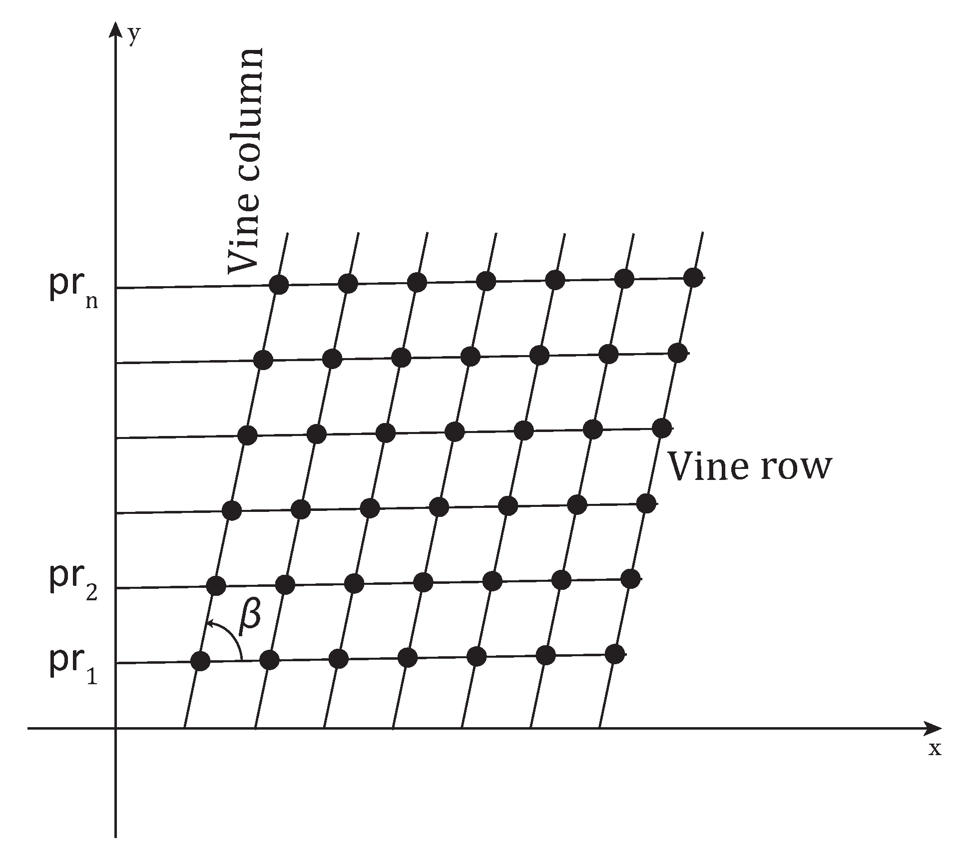
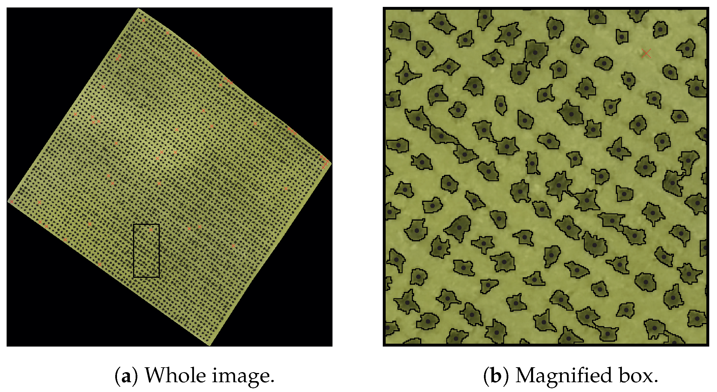
The images, provided by Château Kefraya vineyards in Lebanon, were acquired on 13 June 2017 using a Sensefly eBee fixed-wing UAV at an average flying height of 300 using a Sony DSC-WX220. The captured raw images have an average ground sample distance (GSD) of . The camera has a 1/2.3” sensor with a resolution of 4896 × 3672 pixels. The raw images are processed using Pix4Dmapper to generate an orthophoto with a resolution of . The image of each parcel is clipped from the original orthophoto using QGIS. The vines are trained in goblet style along an oriented grid of rows and columns, not necessarily of rectangular shape, with inter-row and inter-column spacing (see Figure 1). The acquired images are flipped, so that the y-axis starts at the bottom of the image and runs to the top in order to facilitate the migration between image coordinates and geographic coordinates. Table 1 shows the list of the parcels used as research data. It includes the parcel’s ID, its area, and the coordinates of its center in the UTM 36N coordinate reference system. Parcel 59B (see Figure 1) is used to illustrate the different steps of the proposed method.
2.2. Proposed Method
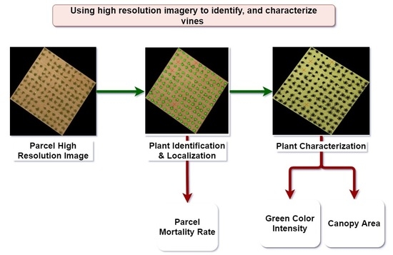
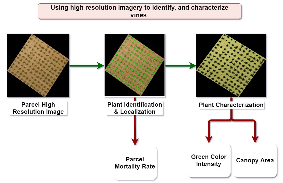
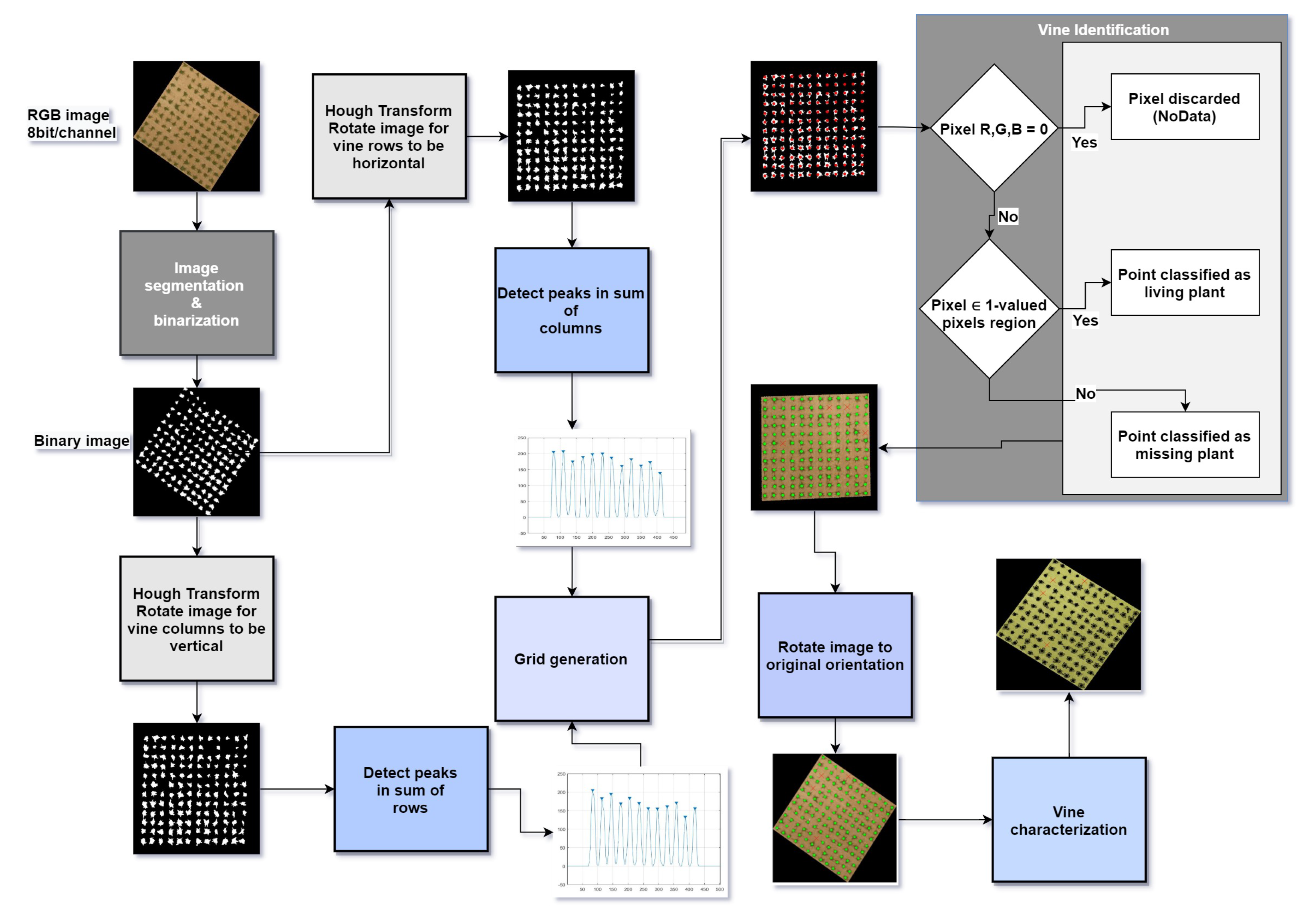
The proposed method, illustrated in Figure A1, is composed of two major stages: vine identification and vine characterization.
The purpose of the vine identification stage is to identify and localize living and missing plants. First, the RGB image is segmented using K-means clustering then binarized by setting all pixels representing vines to 1, and all other pixels to 0. Then, the image is rotated properly to facilitate the localization of vine rows and columns. Using the vine rows and columns locations, a grid is generated over the image. A grid point may correspond to a living vine, a missing vine, or a bare point localized outside the plantable area.
The purpose of the vine characterization stage is to identify the pixels of each living plant. Using the locations of living vines obtained from the previous stage, a marker-controlled watershed transform is applied on the image in order to detect each plant as a solitary object even if it overlaps with other plants.
2.2.1. Vine Identification
In order to achieve vine identification; first, the image is segmented then binarized, and then the binary image is rotated and the locations of vine rows and columns are calculated. Finally, living and missing plants are identified and localized.
2.2.1.1. Image Segmentation and Binarization
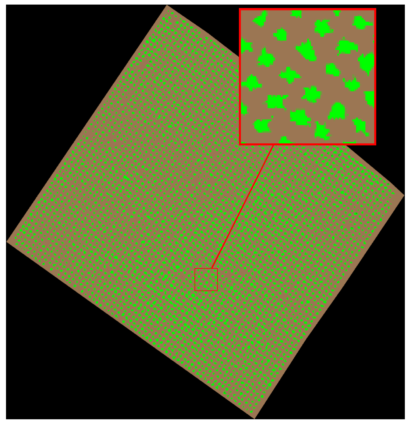
The K-means clustering algorithm [18] is applied on the RGB-coded parcel image in order to segment it and identify pixels belonging to three categories: vines, soil, and no-data. The K-means clustering is an unsupervised learning method that is able to operate on data without prior knowledge of their structure. However, the number of clusters must be given a priori. The K-means algorithm is applied on the parcel image with a number of clusters equal to 3 resulting in allocating the pixels to 3 segments: the vines segment, the soil segment, and the no-data segment (see Figure 2).
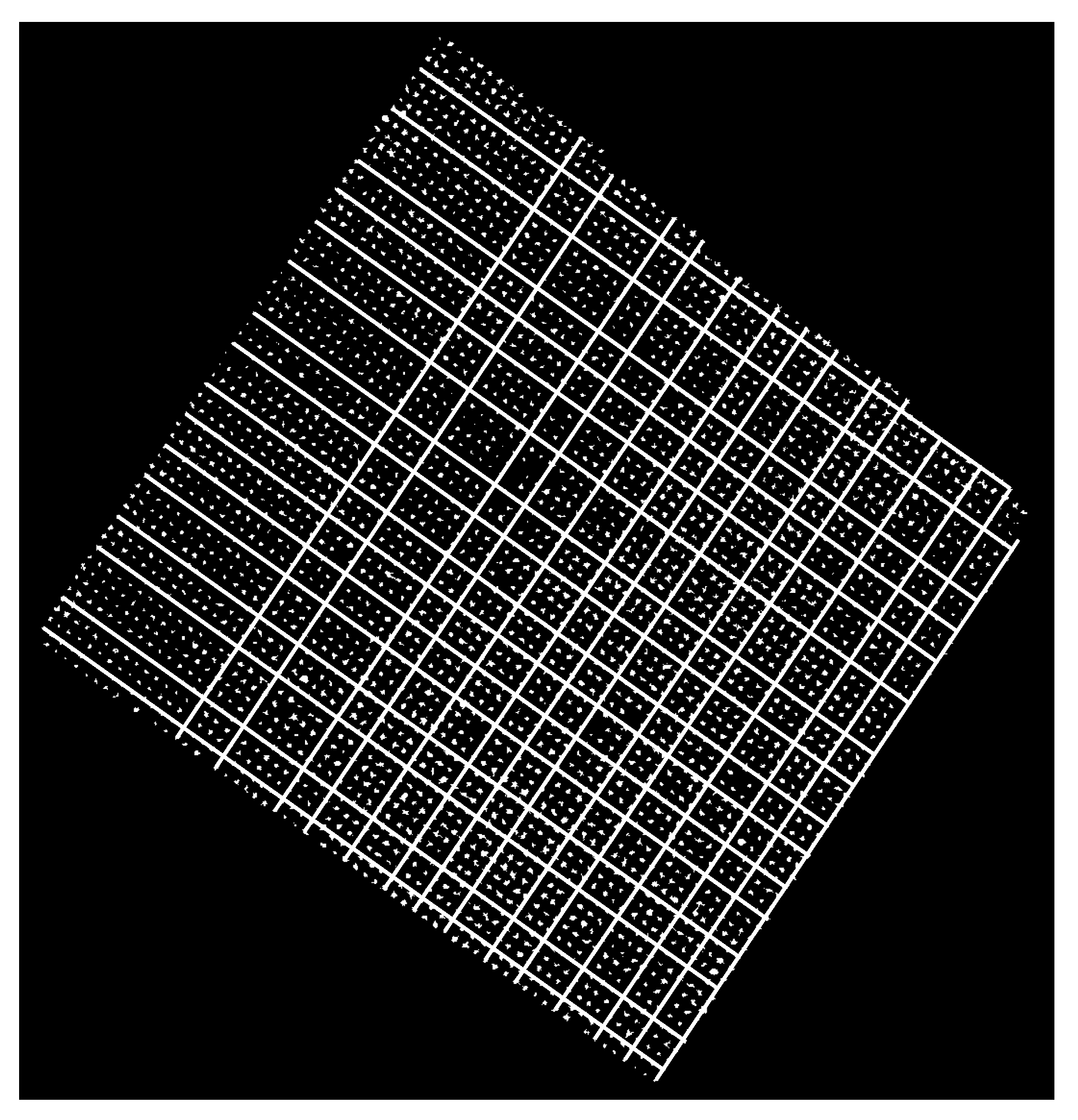
The image binarization is achieved by setting to 1 all pixels belonging to the vine segment and to 0 all other pixels (see Figure 3). The binary version of the parcel image is denoted . Following observations performed on the images, clusters of less than are removed from the binary image for being considered as unwanted data. This area is equivalent to a number of pixels expressed using the ground sample distance (GSD) expressed as:
2.2.1.2. Image Rotation
The Hough transform [19] is used to detect major lines in the image and consequently detect both grid angles. It is an easy and fast method that yields accurate results.
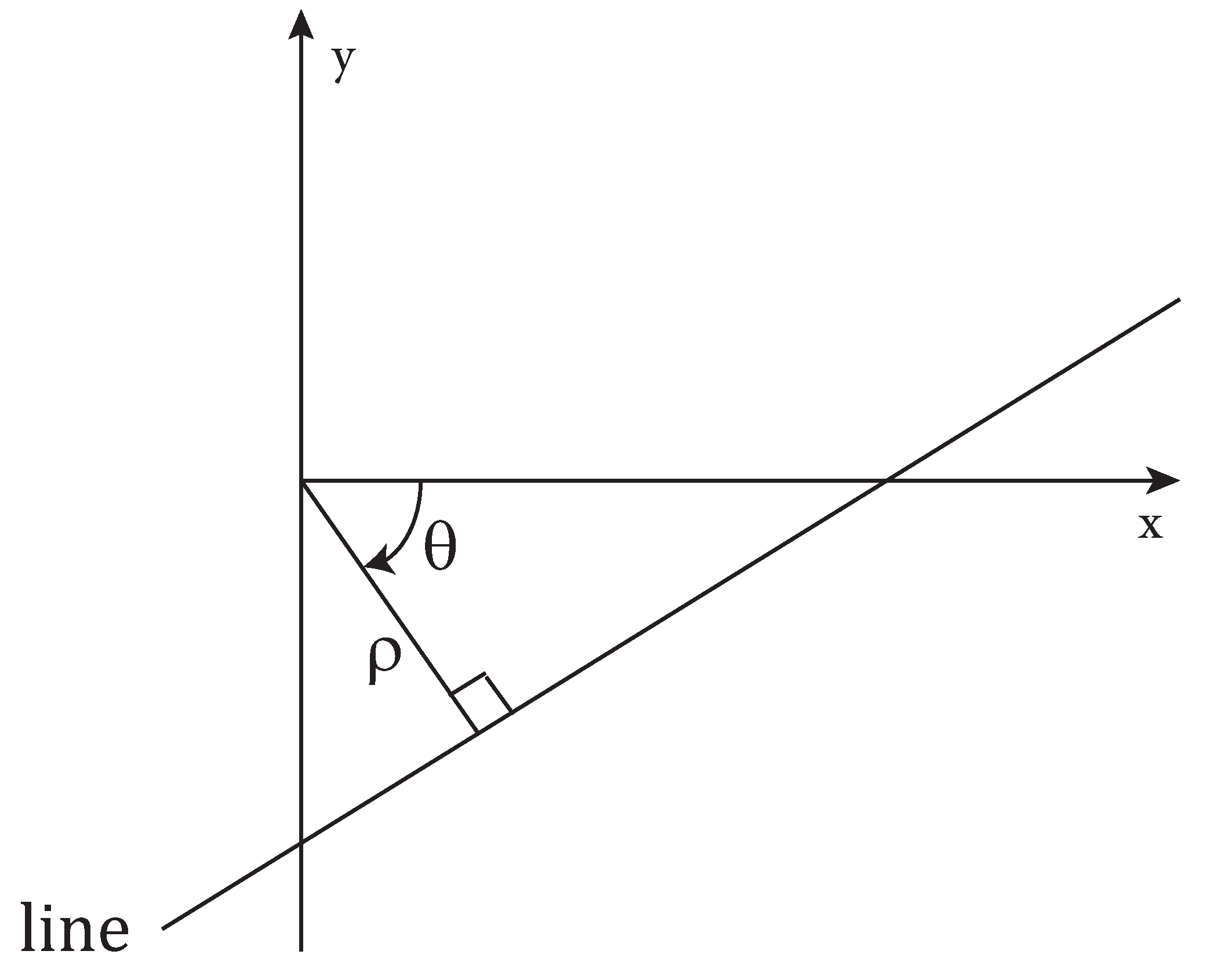
Let us consider the parametric representation of a line in terms of and angle:
where is the angle formed by the line’s normal with the x-axis and its algebraic distance from the origin (see Figure 4).
If angle is restricted to an interval of length , the normal parameters for a line are unique. A point in the x–y plane corresponds to a sinusoidal curve in the – plane, and collinear points in the x–y plane correspond to curves intersecting at the same point in the – plane. Such points are called peaks.
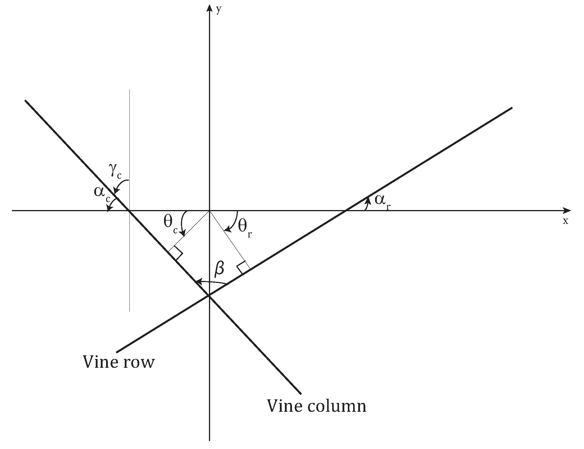
The most frequent negative angle and the most frequent positive angle are determined and denoted and , respectively. The angle formed by a vine row, and the x-axis is calculated in Equation (3) and the angle formed by a vine column and the y-axis is calculated in Equation (4).
Consequently, the angle formed by a vine row and a vine column is:
where is the angle formed by a vine column and the x-axis.
Figure 5 illustrates the calculated angles. It should be noted that in all the figures of this section the y-axis is oriented upwards following the orientation of the image vertical axis (see Section 2.1).
In order to obtain optimal results when using the Hough transform, clusters representing overlapping vines in the binary images must be eroded to isolate vines. That is why morphological erosion [20], with a diamond structuring element of size 2, is performed on the binary images of all analyzed parcels. The Hough transform is applied on the eroded binary image by varying the angle between −90° and 89° with an increment of 0.5°.
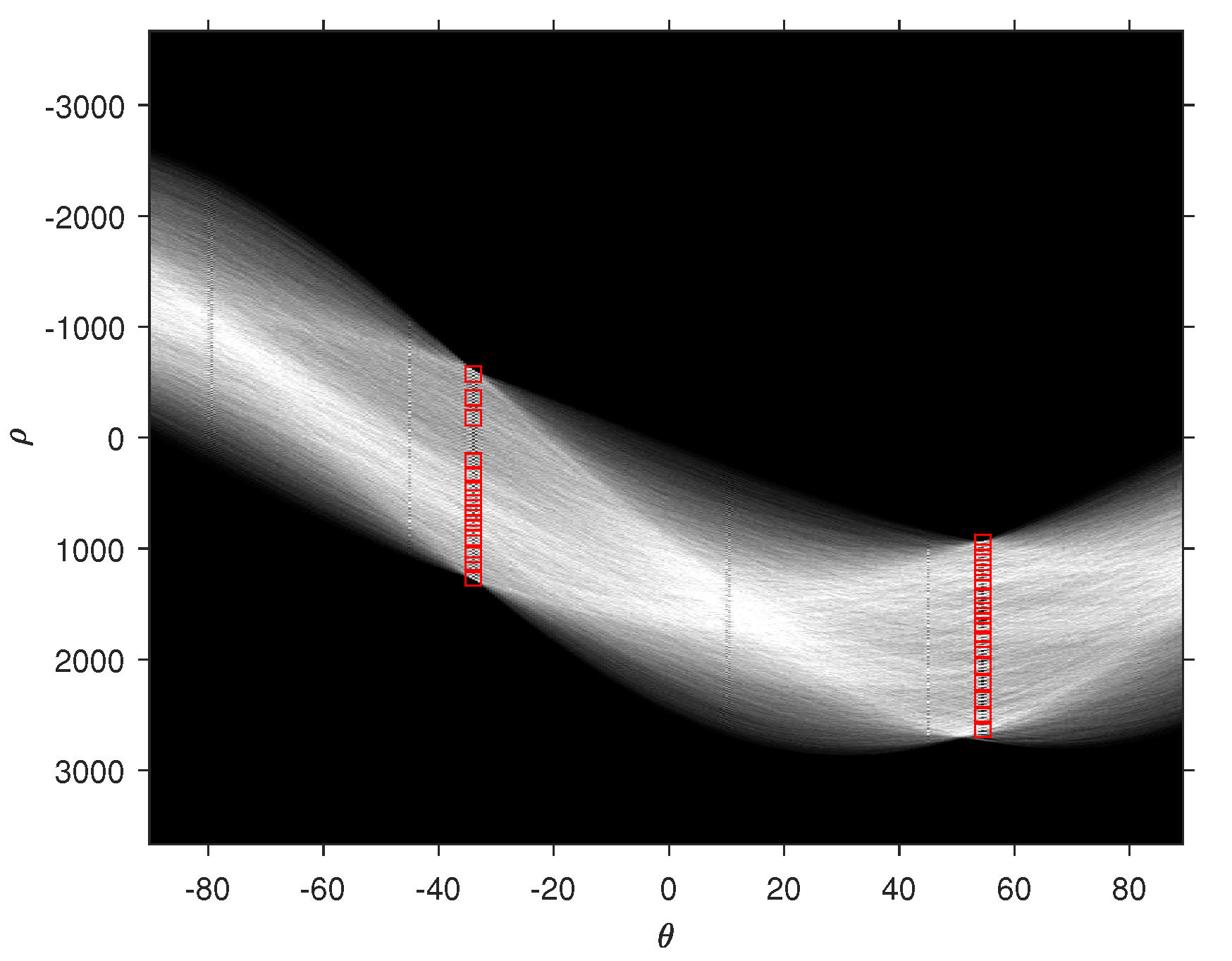
Figure 6 shows the – plane where 30 peaks are identified when the Hough transform is applied on the binary image of Parcel 59B.
The most frequent negative angle is and the most frequent positive angle is yielding , and . is the angle by which the image must be rotated clockwise around its center for the rows of vines to be horizontal. The resulting obtained image is denoted . is the angle by which the image must be rotated clockwise around its center for the columns of vines to be vertical. The obtained image is denoted . Figure 7 shows the binary image of Parcel 59B overlayed with lines relative to and angles.
2.2.1.3. Living and Missing Vine Identification
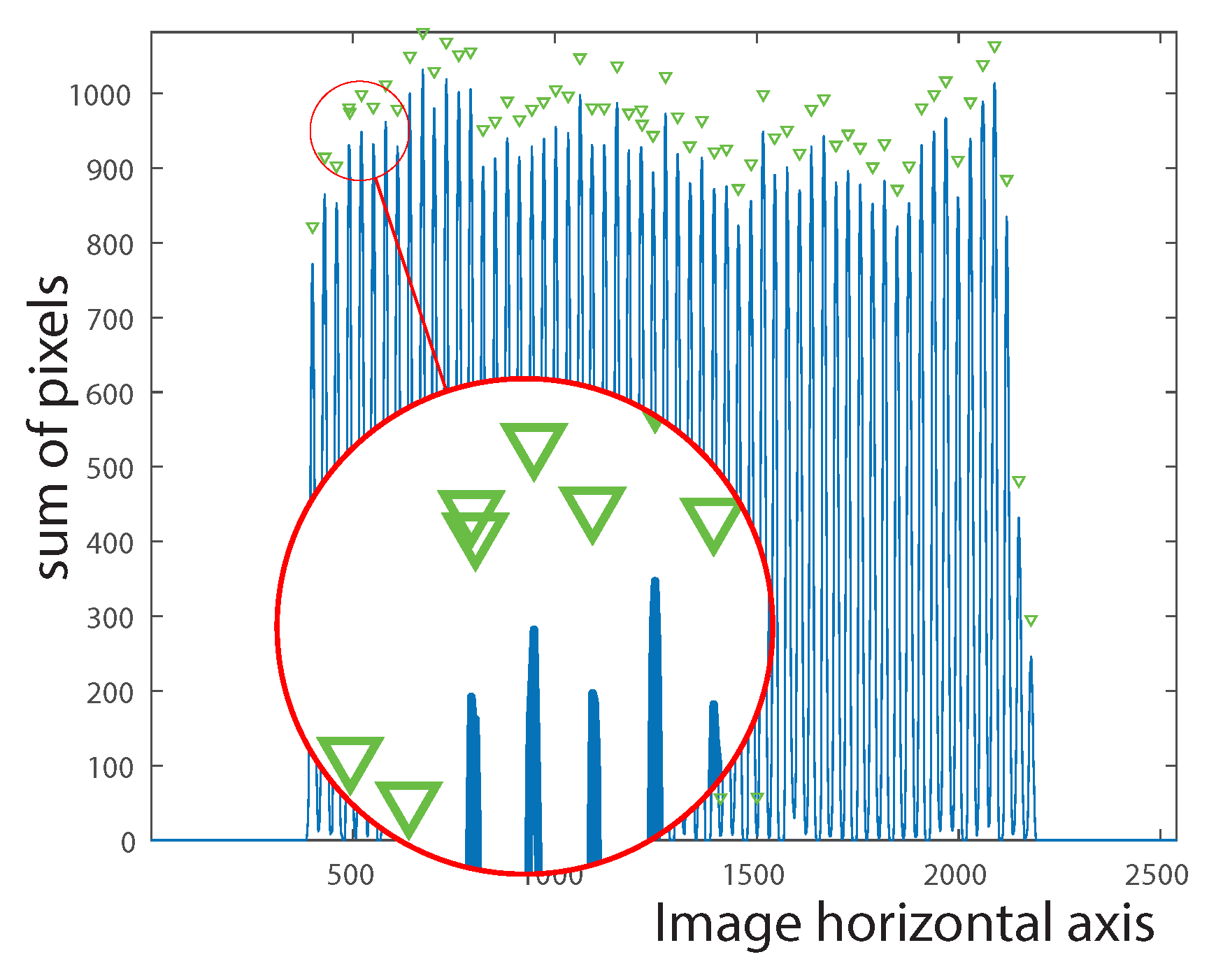
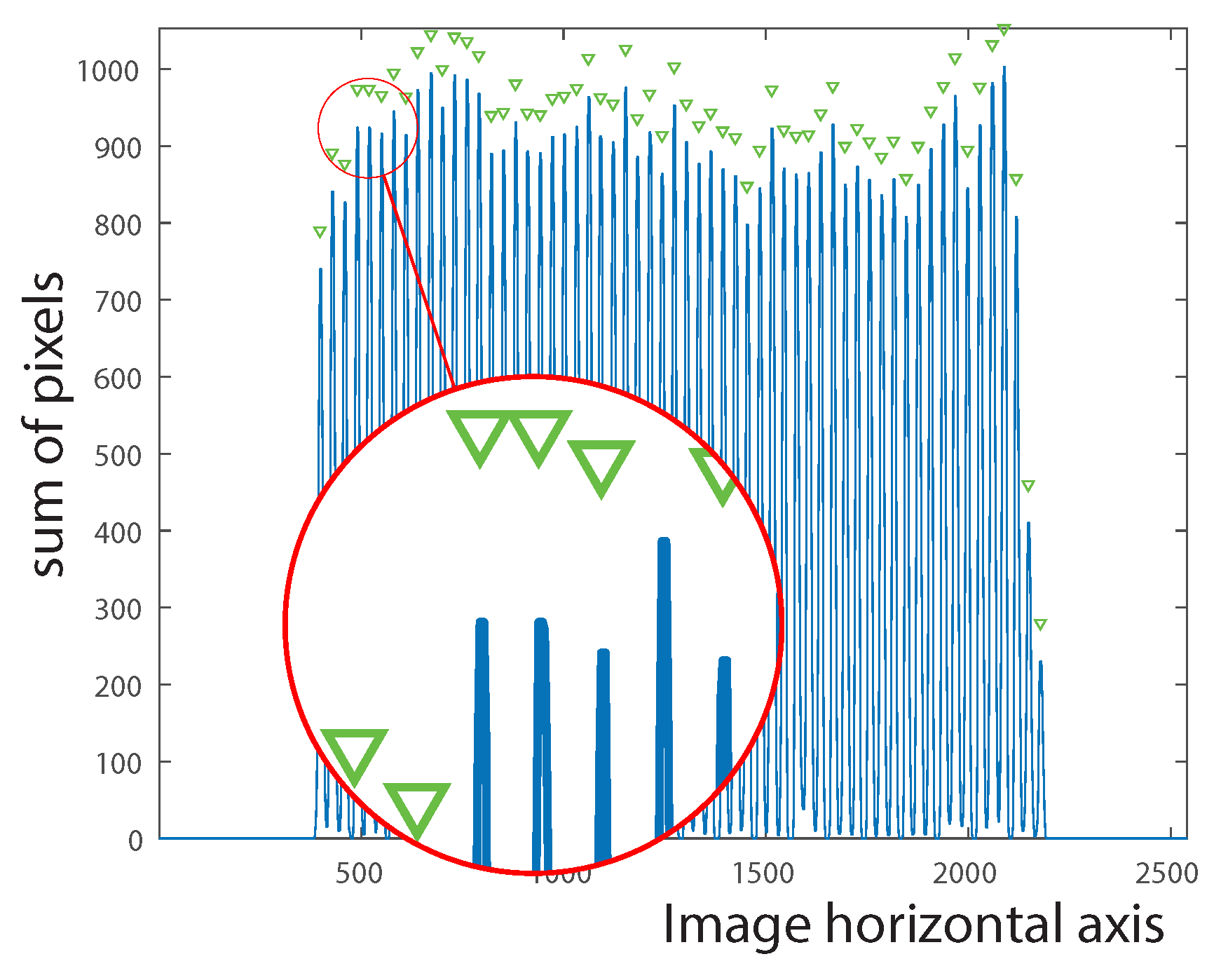
Considering the fact that all vines are represented by 1-valued pixels in the binary images, the vine locations can be easily calculated by summing the columns in the image and the rows in the image. The peak locations in the sum of rows signal constitute a vector of length n that indicates the placement of the vine points along the vertical axis. Similarly, the peak locations in the sum of columns signal constitute a vector of length m that indicates the placement of the vine points along the horizontal axis. These signals may contain noise as a result of vine overlapping. For this reason, the median filter (Equation (6)) is applied on both signals in order to smooth them and subsequently eliminate unnecessary peaks (see Figure 8 and Figure 9).
where is the input signal and is the output signal. Each is the median of samples of the input signal centered at t, where N is the filter length set to 5. The most frequent distances between the peaks of the sum of columns signal and of the sum of rows signal define the inter-column spacing and the inter-row spacing, respectively.
The presence of weeds between vine rows and vine columns leads to faulty peaks. To resolve this issue, a minimal distance between peaks is imposed. It is equivalent to 2/3 of the inter-column spacing for the sum of columns signal and 2/3 of the inter-row spacing in the sum of rows signal.
The peak location vectors (illustrated in Figure 10), and (illustrated in Figure 11) are used to generate a two-dimensional grid of m columns and n rows to be displayed over the image where the vine columns are vertical (see Figure 11). A grid point is defined as with and . is the ordinate of the point obtained after rotating the point counter-clockwise by according to the following equations:
where x could be any positive value, is the center of the image, is the angle calculated in Equation (5), and is the rotation matrix defined as:
In the case of Parcel 59B, and .
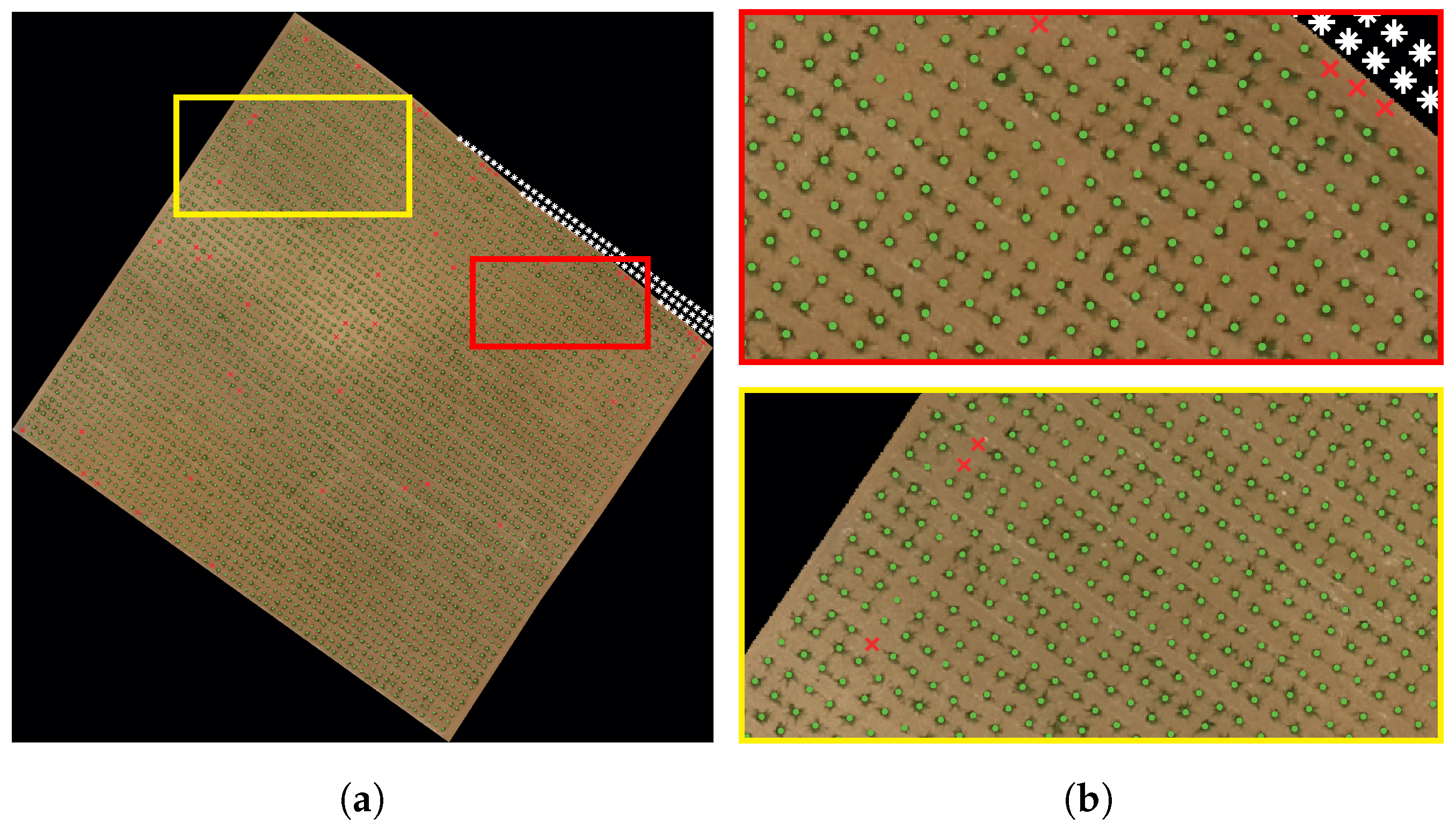
The grid points displayed over the image represent either a living vine point, a missing vine point or a bare point. Points having their red, green, and blue components equal to 0 belong to the no-data segment; they are considered as bare points and, therefore, discarded. For all remaining points, a rectangle window, centered on the considered point, is cropped from the image. The length and width of the rectangle are equal to half of the inter-column and of the inter-row distances, respectively. Regions of 1-valued pixels are sought inside this window. If such regions are found, the grid point is classified as a living vine point and is moved to the center of the closest region which ensures that the grid point is as close as possible to the vine’s center. Otherwise, the grid point is classified as a missing vine point since pixels in its neighborhood are 0-valued.
The final grid points to be displayed over the original parcel image are rotated counter-clockwise by calculated as follows:
Figure 12 shows the parcel image overlayed with the generated grid composed of the three types of points: missing vine point (x), living vine point (•), and bare point (*).
2.2.2. Vine Characterization
The purpose of this part is to characterize each vine by identifying its pixels. Due to their big size, some vines may overlap and, therefore, may be considered as one object as in some classical segmentation methods. The watershed transform [21,22] is able to segment a binary image while identifying contiguous regions as separate objects. It considers the image to be processed as a topographic surface where a pixel brightness represents its height. The watershed algorithm simulates a water flooding on this surface starting from the minima (darkest pixels). It prevents water merging by building dams. At the end of the flooding process, catchment basins are formed, each related to one minimum. These basins are separated by watershed lines defined by the dams. Therefore, pixels of the image are partitioned into catchment basins or watershed lines. The watershed transform in its primary algorithm may lead to an over-segmentation of the image. For this reason, a marker-controlled watershed algorithm is proposed [23]. It consists of detecting markers that constitute the only source of flooding. Two kinds of markers are used: the object related markers that uniquely define each object and the background related markers that surround the objects.
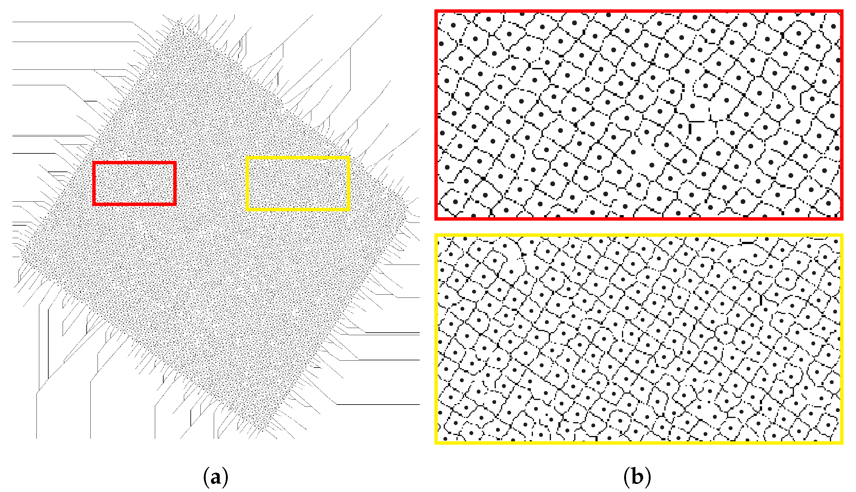
In this study, the marker-controlled watershed transform is applied on the gradient of the grayscale parcel image. First, using the vine clusters identified in the K-means process (see Section 2.2.1.1), the corresponding red channel pixels are extracted from the RGB image to create a grayscale image. Then, the gradient of the grayscale image is produced. The objects or vine related markers are the living vine points detected in Section 2.2.1.3. The background markers are computed by applying the watershed transform on the distance transform of the binary image (). The distance transform replaces each pixel in the binary image by its distance to the nearest non-zero pixel. The background related markers are the 0-valued pixels of the resulting watershed transform. The black dots in Figure 13 represent the vines, while the black lines represent the background markers. The gradient image is modified by morphological reconstruction so that the only regional minima are the pixels considered as vine and background markers [24]. Figure 14 shows the parcel image overlayed with the result of the watershed segmentation on the modified gradient image. It is apparent that the vines, identified with black dots, are well delineated, even the overlapping ones.
2.3. Semantic Segmentation
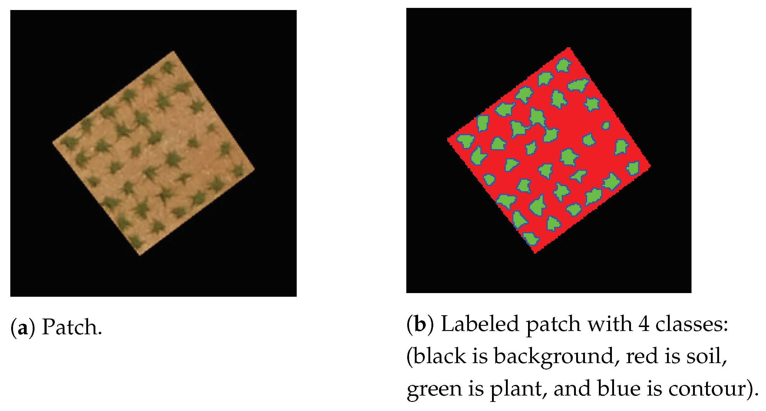
Semantic segmentation is the task of assigning a class to every pixel in the image. It is used in this study for comparison purposes with K-means segmentation. Many deep learning algorithms have been proposed recently for semantic segmentation [25,26]. The model used for semantic segmentation is the Deeplabv3plus [27] based on the pretrained convolutional neural network ResNet-18. The training of the network is performed using patches. In total, 591 patches of 224 × 224 pixels (the minimal size required by ResNet-18) are extracted from the images of the different parcels. Each learning sample consists of a patch and its corresponding labeled patch, where pixels belong to four classes: the background class, the soil class, the plant class, and the contour class. Trials with only three classes (background, soil, and plant) yielded poor results because overlapping vines are considered as one object. Adding the contour class reduced vine overlapping considerably by isolating vines that might connect. Figure 15 shows a training sample consisting of a patch and its labeled version. The optimization algorithm used for training is the stochastic gradient descent with momentum (SGDM). The maximum number of epochs is set to 40. The learning rate uses a piecewise schedule. The initial learning rate is set to 0.0001. The learning rate is reduced by a factor of 0.3 every 10 epochs [28].
3. Results
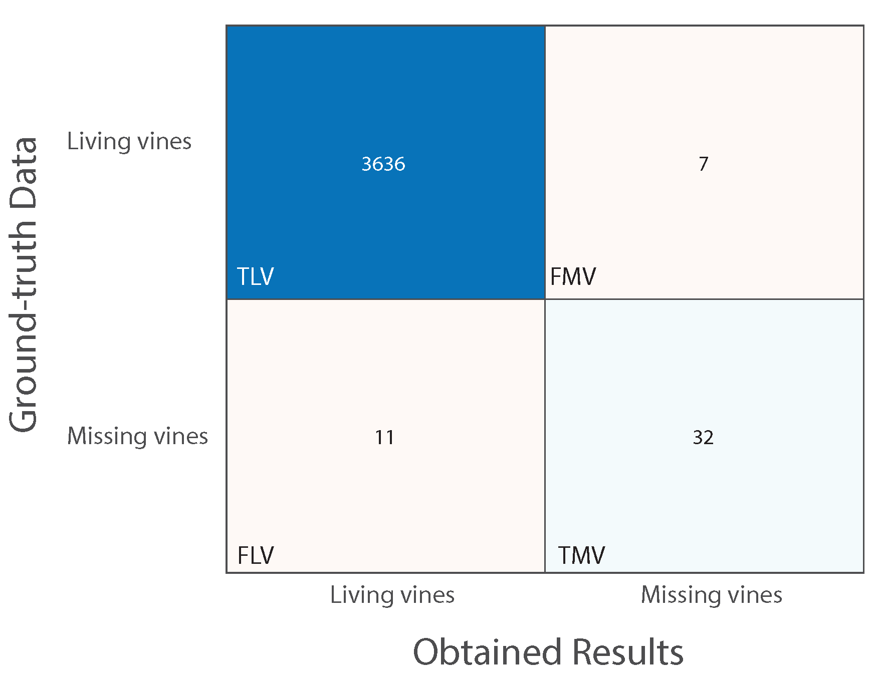
In order to assess the proposed method, recent ground-truth manual counting is performed on Parcel 59B. Moreover, for all parcels listed in Table 1, a desktop GIS software is used to manually digitize the vine locations and visually estimate missing vine locations using row and column intersections. For each digitized point, a row and column number is assigned while an attribute of 1 is given to represent a vine and 0 a missing vine. In each case and for each parcel, a matching matrix is computed showing the numbers of truly identified living vines (TLV) and missing vines (TMV), and the numbers of misidentified living vines (FLV) and missing vines (FMV). The accuracy of the proposed method is quantified by calculating the accuracy of missing vines identification (AMV) computed in Equation (11), the accuracy of living vines identification (ALV) computed in Equation (12), and the overall accuracy (ACC) computed in Equation (13).
3.1. Assessment of Proposed Method Compared to Ground-Truth Data
Table 2 shows the comparison between the ground-truth data and the results obtained by applying the proposed method on Parcel 59B. It compares the number of vine rows and the number of living and missing vines in both cases. It also shows the mortality rate in both cases calculated as in Equation (14).
Figure 16 displays the obtained matching matrix when assessing the proposed method against Parcel 59B’s ground-truth data. Regarding accuracy computation, the accuracy of missing vine identification (AMV) is equal to 74.42%, the accuracy of living vine identification (ALV) is equal to 99.81% and the overall accuracy (ACC) is equal to 99.51%.
3.2. Assessment of Proposed Method Compared to On-Screen Vine Identification
Table 3 shows the values of TLV, TMV, FLV, and FMV. It also shows the accuracy of living vine identification (ALV) (Equation (12)), the accuracy of missing vine identification (AMV) (Equation (11)) and the overall accuracy (ACC) (Equation (13)).
High accuracy values are obtained when comparing the yielded results with ground-truth data and on-screen vine identification. Accuracy values (ACC) exceed 95% for all parcels proving that the proposed method succeeds in identifying missing and living vines. However, the obtained AMV values are lower than the ALV values due to the fact that some small vines, considered dead with on-screen identification, are classified as living vines. Lower accuracy values are obtained when the results are compared with ground-truth data because the parcel may have witnessed many changes since 2017, when the images were taken.
Regarding vine characterization, the pixels of each vine are identified (see Section 2.2.2). Consequently, further inspection on the size, shape, and green color intensity of each vine can be easily performed. For example, 9.85% of the vines in Parcel 59B have a small size (less than ) and may require special treatment. Table 4 shows the percentage of vines having a size less than , between and , and greater than in each parcel. Parcel 60D has the largest percentage of big vines while Parcel 58C has the largest percentage of small vines.
3.3. Comparison with Semantic Segmentation
In order to test the trained DeepLab3vplus model (see Section 2.3), the image of Parcel 59B (Figure 1) is presented to the network after resizing it to pixels where and are the closest multiples of 224 to the number of lines and the number of columns of the image, respectively. Even if the size of the test image is different than those of the learning samples, DeepLabv3plus still succeeds in classifying the pixels, as long as the size of the features (vines) are close to the ones learned by the network. Figure 17 shows the image of Parcel 59B overlayed with the semantic segmentation results using the trained Deeplabv3plus model. It is obvious that the pixels of the image are well classified among four segments: background, soil, plant, and contour.
By setting to one all pixels belonging to the plant segment and to zero all remaining pixels, a binary image is obtained where most of the vines form solitary objects. By applying proper image rotation (Section 2.2.1.2) and plant identification (Section 2.2.1.3), the living and missing vines are identified giving an overall accuracy of ACC = 99.5% (Equation (13)) when these results are assessed with ground-truth data.
Table 5 shows a comparison between the results obtained from the proposed method, those obtained by applying CNN-based Semantic Segmentation followed by plant identification, and those obtained from manual counting on the ground.
4. Discussion
The proposed method succeeded in identifying the living and missing vines of the analyzed parcels with high accuracy (exceeding 95%) giving the possibility to calculate a precise mortality rate. Converting image coordinates to geographical coordinates is possible since each parcel image is a geoTIFF image, which means it is fully georeferenced. A proper intervention on the parcels presenting high mortality rate along with the possibility to locate any missing vine geographically in GIS will increase the parcel’s productivity. Moreover, identifying the pixels of each vine in the context of vine characterization helps detecting any disease that might affect the vines by investigating their size, their shape, and the intensity of their green color. Using CNN-based semantic segmentation instead of K-means clustering yielded quite similar results in terms of vine identification. However, it is a supervised method that requires a large number of learning samples to train the network, whereas the proposed method is unsupervised, requiring only the image as input.
Despite its numerous advantages, this method has some limitations if the vine geometric distribution over the plot grid presents major irregularities. In this case, the sum of rows and the sum of columns signals will fail in detecting the presence of vine rows and vine columns. Additionally, it will be difficult to apply a specific rule for the localization of missing vines. Another limitation may arise from the presence of none-vine plants between the vines that are more likely to belong to the same vine cluster when K-means is used for image segmentation. In this case, one might have recourse to convolutional neural networks based methods that are able to distinguish the vine plants from other plants if the network is well trained. For example, instance segmentation is a potential solution. It produces bounding boxes that surround each instance while recognizing its pixels. Nevertheless, these methods are supervised and need a big number of learning samples that might be unavailable.
5. Conclusions
In this paper, a complete study is presented for vine identification and characterization in goblet-trained vine parcels by analyzing their images. In the first stage, the location of each living and missing plant is depicted. In the second stage, the pixels belonging to each plant are recognized. The results obtained when applying the proposed method on 10 parcels are encouraging and prove its validity. The accuracy of missing and living plants identification exceeds 95% when comparing the obtained results with ground-truth and on-screen vine identification data. Moreover, characterizing each vine helps identifying the leaf size and color for potential disease detection. Additionally, it is an automated method that operates on the image without prior training. Replacing K-means segmentation with CNN-based semantic segmentation yielded good results. However, it is a supervised method that requires network tuning and training.
Parcels delineation methods proposed in literature may be used to automatically crop the parcels images in order to provide a complete and automatic solution for the vineyard digitization and characterization. The success of this method depends on the regular geometric distribution of the vines and on the absence of non-vine plants. Otherwise, supervised methods like instance segmentation might be used for vine identification and characterization with the condition that a learning dataset is available.
Author Contributions
Conceptualization, C.H.; methodology, C.H. and G.G.; software, C.H.; validation, C.H. and G.G.; resources, M.K.S. and Y.G.C.; data curation, C.H. and G.G.; writing—original draft preparation, C.H.; writing—review and editing, C.H., G.G., M.K.S. and Y.G.C.; supervision, C.H., Y.G.C. and M.K.S.; project administration, C.H., Y.G.C. and M.K.S.; funding acquisition, Y.G.C. and M.K.S. All authors have read and agreed to the published version of the manuscript.
Funding
This research was funded by the Lebanese National Council for Scientific Research (CNRS) and the Saint-Joseph University (USJ) in Beirut.
Institutional Review Board Statement
Not applicable.
Informed Consent Statement
Not applicable.
Data Availability Statement
Restrictions apply to the availability of these data. Data was obtained from Château Kefraya and are available with their permission.
Acknowledgments
The authors are extremely grateful to the management of Château Kefraya for all the technical support they provided.
Conflicts of Interest
The authors declare no conflict of interest.
Abbreviations
The following abbreviations are used in this manuscript:
| Binary parcel image | |
| Binary parcel image where the vine columns are vertical | |
| Binary parcel image where the vine rows are horizontal | |
| TLV | Number of truly identified living vines |
| TMV | Number of truly identified missing vines |
| FLV | Number of misidentified living vines |
| FMV | Number of misidentified missing vines |
| AMV | Missing vine identification accuracy |
| ALV | Living vine identification accuracy |
| ACC | Vine identification accuracy |
Appendix A
Figure A1.
Proposed method flowchart.

References
- Matese, A.; Di Gennaro, S. Technology in precision viticulture: A state of the art review. Int. J. Wine Res. 2015, 7, 69–81. [Google Scholar] [CrossRef] [Green Version]
- Sassu, A.; Gambella, F.; Ghiani, L.; Mercenaro, L.; Caria, M.; Pazzona, A.L. Advances in Unmanned Aerial System Remote Sensing for Precision Viticulture. Sensors 2021, 21, 956. [Google Scholar] [CrossRef] [PubMed]
- Delenne, C.; Rabatel, G.; Deshayes, M. An Automatized Frequency Analysis for Vine Plot Detection and Delineation in Remote Sensing. IEEE Geosci. Remote Sens. Lett. 2008, 5, 341–345. [Google Scholar] [CrossRef] [Green Version]
- Delenne, C.; Durrieu, S.; Rabatel, G.; Deshayes, M. From pixel to vine parcel: A complete methodology for vineyard delineation and characterization using remote-sensing data. Comput. Electron. Agric. 2010, 70, 78–83. [Google Scholar] [CrossRef] [Green Version]
- Comba, L.; Gay, P.; Primicerio, J.; Ricauda Aimonino, D. Vineyard detection from unmanned aerial systems images. Comput. Electron. Agric. 2015, 114, 78–87. [Google Scholar] [CrossRef]
- Primicerio, J.; Caruso, G.; Comba, L.; Crisci, A.; Gay, P.; Guidoni, S.; Genesio, L.; Ricauda Aimonino, D.; Primo Vaccari, F. Individual plant definition and missing plant characterization in vineyards from high-resolution UAV imagery. Eur. J. Remote Sens. 2017, 50, 179–186. [Google Scholar] [CrossRef]
- Chanussot, J.; Bas, P.; Bombrun, L. Airborne remote sensing of vineyards for the detection of dead vine trees. In Proceedings of the International Geoscience and Remote Sensing Symposium (IGARSS), Seoul, Korea, 29 July 2005; Volume 5, pp. 3090–3093. [Google Scholar] [CrossRef]
- Poblete-Echeverría, C.; Olmedo, G.F.; Ingram, B.; Bardeen, M. Detection and Segmentation of Vine Canopy in Ultra-High Spatial Resolution RGB Imagery Obtained from Unmanned Aerial Vehicle (UAV): A Case Study in a Commercial Vineyard. Remote Sens. 2017, 9, 268. [Google Scholar] [CrossRef] [Green Version]
- Carbonneau, A.; Cargnello, G. Architectures de la Vigne et Systèmes de Conduite; Pratiques Vitivinicoles, Dunod: Paris, France, 2003. [Google Scholar]
- Robbez-Masson, J.M.; Foltête, J.C. Localising missing plants in squared-grid patterns of discontinuous crops from remotely sensed imagery. Comput. Geosci. 2005, 31, 900–912. [Google Scholar] [CrossRef]
- Hayat, S.; Kun, S.; Tengtao, Z.; Yu, Y.; Tu, T.; Du, Y. A Deep Learning Framework Using Convolutional Neural Network for Multi-Class Object Recognition. In Proceedings of the 2018 IEEE 3rd International Conference on Image, Vision and Computing (ICIVC), Chongqing, China, 27–29 June 2018; pp. 194–198. [Google Scholar]
- Girshick, R.; Donahue, J.; Darrell, T.; Malik, J. Rich Feature Hierarchies for Accurate Object Detection and Semantic Segmentation. In Proceedings of the 2014 IEEE Conference on Computer Vision and Pattern Recognition, Columbus, OH, USA, 23–28 June 2014; pp. 580–587. [Google Scholar]
- Girshick, R. Fast R-CNN. In Proceedings of the 2015 IEEE International Conference on Computer Vision (ICCV), Santiago, Chile, 7–13 December 2015; pp. 1440–1448. [Google Scholar]
- Redmon, J.; Divvala, S.; Girshick, R.; Farhadi, A. You Only Look Once: Unified, Real-Time Object Detection. In Proceedings of the 2016 IEEE Conference on Computer Vision and Pattern Recognition (CVPR), Las Vegas, NV, USA, 27–30 June 2016; pp. 779–788. [Google Scholar]
- Ren, S.; He, K.; Girshick, R.; Sun, J. Faster R-CNN: Towards Real-Time Object Detection with Region Proposal Networks. IEEE Trans. Pattern Anal. Mach. Intell. 2017, 39, 1137–1149. [Google Scholar] [CrossRef] [PubMed] [Green Version]
- Chen, L.; Papandreou, G.; Kokkinos, I.; Murphy, K.; Yuille, A.L. DeepLab: Semantic Image Segmentation with Deep Convolutional Nets, Atrous Convolution, and Fully Connected CRFs. IEEE Trans. Pattern Anal. Mach. Intell. 2018, 40, 834–848. [Google Scholar] [CrossRef] [PubMed]
- He, K.; Gkioxari, G.; Dollár, P.; Girshick, R. Mask R-CNN. In Proceedings of the 2017 IEEE International Conference on Computer Vision (ICCV), Venice, Italy, 22–29 October 2017; pp. 2980–2988. [Google Scholar]
- Duda, R.O.; Hart, P.E.; Stork, D.G. Pattern Classification, 2nd ed.; Wiley: New York, NY, USA, 2001. [Google Scholar]
- Duda, R.O.; Hart, P.E. Use of the Hough Transformation to Detect Lines and Curves in Pictures. Commun. ACM 1972, 15, 11–15. [Google Scholar] [CrossRef]
- Batchelor, B.G.; Waltz, F.M. Morphological Image Processing. In Machine Vision Handbook; Batchelor, B.G., Ed.; Springer: London, UK, 2012; pp. 801–870. [Google Scholar] [CrossRef]
- Beucher, S.; Lantuéjoul, C. Use of Watersheds in Contour Detection. In Proceedings of the International Workshop on Image Processing: Real-time Edge and Motion Detection/Estimation, Rennes, France, 17–21 September 1967; Volume 132. [Google Scholar]
- Meyer, F. Topographic distance and watershed lines. Signal Process. 1994, 38, 113–125. [Google Scholar] [CrossRef]
- Beucher, S. The watershed transformation applied to image segmentation. Scanning Microsc. Suppl. 1992, 28, 299–314. [Google Scholar]
- The MathWorks. Image Processing Toolbox; MathWorks: Natick, MA, USA, 2019. [Google Scholar]
- Long, J.; Shelhamer, E.; Darrell, T. Fully convolutional networks for semantic segmentation. In Proceedings of the 2015 IEEE Conference on Computer Vision and Pattern Recognition (CVPR), Boston, MA, USA, 7–12 June 2015; pp. 3431–3440. [Google Scholar] [CrossRef] [Green Version]
- Noh, H.; Hong, S.; Han, B. Learning Deconvolution Network for Semantic Segmentation. In Proceedings of the 2015 IEEE International Conference on Computer Vision (ICCV), Santiago, Chile, 7–13 December 2015; pp. 1520–1528. [Google Scholar] [CrossRef] [Green Version]
- Chen, L.C.; Zhu, Y.; Papandreou, G.; Schroff, F.; Adam, H. Encoder-Decoder with Atrous Separable Convolution for Semantic Image Segmentation. In Proceedings of the European Conference on Computer Vision (ECCV), Munich, Germany, 8–14 September 2018; Ferrari, V., Hebert, M., Sminchisescu, C., Weiss, Y., Eds.; Lecture Notes in Computer Science. Springer: Cham, Switzerland, 2018; Volume 11211, pp. 833–851. [Google Scholar] [CrossRef] [Green Version]
- The MathWorks. Deep Learning Toolbox; MathWorks: Natick, MA, USA, 2019. [Google Scholar]
Figure 1.
Goblet trained parcel. (a): whole image, (b): magnified boxes.

Figure 2.
Three segments image: vines (green), soil (brown), and no-data (black).

Figure 3.
Binary image showing vine pixels with a value of 1 in white.

Figure 4.
Parametric representation of a line.

Figure 5.
Grid rotation angles.

Figure 6.
30 Hough peaks corresponding to and .

Figure 7.
Hough lines drawn along some of the vine columns and rows.

Figure 8.
Original signal where overlapping peaks may occur.

Figure 9.
Smoothed signal by applying the median filter.

Figure 10.
Horizontal vine rows.

Figure 11.
Vertical vine columns.

Figure 12.
Living and missing vine identification. (a): whole image, (b): magnified boxes.

Figure 13.
Vine and background related markers set to regional minima. (a): whole image, (b): magnified boxes.
Figure 13.
Vine and background related markers set to regional minima. (a): whole image, (b): magnified boxes.

Figure 14.
Parcel image overlayed with vine characterization results.

Figure 15.
Learning sample.

Figure 16.
Matching matrix. Assessing the proposed method with Parcel 59B’s ground-truth data.

Figure 17.
Semantic Segmentation results on the image of Parcel 59B.


Table 1.
Parcels used for experiments.
| Parcel | Area | X | Y |
|---|---|---|---|
| 59B | 23,849 m | 755,285 m | 3,726,712 m |
| 59A | 21,061 m | 755,158 m | 3,726,796 m |
| 57A | 10,155 m | 754,148 m | 3,726,945 m |
| 1B | 16,651 m | 753,344 m | 3,726,512 m |
| 58C | 23,225 m | 754,582 m | 3,726,680 m |
| 58D | 6870 m | 754,678 m | 3,726,610 m |
| 60D | 33,778 m | 755,904 m | 3,726,233 m |
| 60A | 25,039 m | 755,523 m | 3,726,573 m |
| 61A | 21,480 m | 755,471 m | 3,726,997 m |
| 10F | 7115 m | 753,318 m | 3,726,843 m |
Table 2.
Vine identification (Parcel 59B). Comparison between the obtained results and ground-truth data.
Table 2.
Vine identification (Parcel 59B). Comparison between the obtained results and ground-truth data.
| Obtained Results | Ground-Truth Data | |
|---|---|---|
| No. of vine rows | 63 | 63 |
| No. of living vines | 3648 | 3643 |
| No. of missing vines | 46 | 43 |
| Mortality rate | 1.24% | 1.17% |
Table 3.
Living and missing vine identification (Parcel 59B). Comparison between the obtained results and the on-screen vine identification.
Table 3.
Living and missing vine identification (Parcel 59B). Comparison between the obtained results and the on-screen vine identification.
| Parcel | TLV | TMV | FLV | FMV | ALV | AMV | ACC |
|---|---|---|---|---|---|---|---|
| 59B | 3643 | 37 | 5 | 0 | 100.00% | 88.10% | 99.86% |
| 59A | 2985 | 212 | 23 | 24 | 99.20% | 90.21% | 98.55% |
| 57A | 1507 | 44 | 9 | 4 | 99.74% | 83.02% | 99.17% |
| 1B | 2011 | 406 | 89 | 38 | 98.15% | 82.02% | 95.01% |
| 58C | 2554 | 851 | 108 | 46 | 98.23% | 88.74% | 95.67% |
| 58D | 736 | 228 | 14 | 25 | 96.71% | 94.21% | 96.11% |
| 60D | 4911 | 217 | 28 | 8 | 99.84% | 88.57% | 99.30% |
| 60A | 3581 | 173 | 25 | 23 | 99.36% | 87.37% | 98.74% |
| 61A | 3161 | 128 | 7 | 1 | 99.97% | 94.81% | 99.76% |
| 10F | 975 | 74 | 24 | 12 | 98.78% | 75.51% | 96.68% |
Table 4.
Percentage of vines according to their size.
| Parcel | Size < 0.69 m | 0.69 m ⩽ Size < 1.38 m | Size ⩾ 1.38 m |
|---|---|---|---|
| 59B | 9.92% | 62.20% | 27.88% |
| 59A | 5.82% | 48.99% | 45.19% |
| 57A | 9.58% | 58.92% | 31.51% |
| 1B | 16.48% | 52.19% | 31.33% |
| 58C | 28.27% | 57.63% | 14.10% |
| 58D | 18.62% | 49.60% | 31.78% |
| 60D | 1.17% | 12.91% | 85.92% |
| 60A | 3.52% | 48.14% | 48.34% |
| 61A | 10.42% | 63.45% | 26.14% |
| 10F | 11.53% | 47.24% | 41.22% |
Table 5.
Vine identification (Parcel 59B). Results from proposed method, semantic segmentation, and ground-truth data.
Table 5.
Vine identification (Parcel 59B). Results from proposed method, semantic segmentation, and ground-truth data.
| Obtained Results | Semantic Segmentation | Ground-Truth Data | |
|---|---|---|---|
| No. of vine rows | 63 | 63 | 63 |
| No. of living vines | 3648 | 3647 | 3643 |
| No. of missing vines | 46 | 47 | 43 |
Publisher’s Note: MDPI stays neutral with regard to jurisdictional claims in published maps and institutional affiliations. |
© 2021 by the authors. Licensee MDPI, Basel, Switzerland. This article is an open access article distributed under the terms and conditions of the Creative Commons Attribution (CC BY) license (https://creativecommons.org/licenses/by/4.0/).
Share and Cite
MDPI and ACS Style
Hajjar, C.; Ghattas, G.; Sarkis, M.K.; Chamoun, Y.G. Vine Identification and Characterization in Goblet-Trained Vineyards Using Remotely Sensed Images. Remote Sens. 2021, 13, 2992. https://doi.org/10.3390/rs13152992
AMA Style
Hajjar C, Ghattas G, Sarkis MK, Chamoun YG. Vine Identification and Characterization in Goblet-Trained Vineyards Using Remotely Sensed Images. Remote Sensing. 2021; 13(15):2992. https://doi.org/10.3390/rs13152992
Chicago/Turabian StyleHajjar, Chantal, Ghassan Ghattas, Maya Kharrat Sarkis, and Yolla Ghorra Chamoun. 2021. "Vine Identification and Characterization in Goblet-Trained Vineyards Using Remotely Sensed Images" Remote Sensing 13, no. 15: 2992. https://doi.org/10.3390/rs13152992
Note that from the first issue of 2016, this journal uses article numbers instead of page numbers. See further details here.