
A Hierarchical Approach to Improve the Interpretability of Causality Maps for Plant-Wide Fault Identification


1
Department of Process Engineering, Faculty of Engineering, Stellenbosch University, Stellenbosch 7600, South Africa
2
Stone Three, Process Monitoring and Diagnosis, 24 Gardner Williams Ave., Paardevlei, Cape Town 7130, South Africa
*
Author to whom correspondence should be addressed.
Minerals 2021, 11(8), 823; https://doi.org/10.3390/min11080823
Submission received: 23 June 2021
/
Revised: 19 July 2021
/
Accepted: 22 July 2021
/
Published: 29 July 2021
(This article belongs to the Special Issue The Application of Machine Learning in Mineral Processing)
Abstract
:Modern mineral processing plants utilise fault detection and diagnosis to minimise time spent under faulty conditions. However, a fault originating in one plant section (PS) can propagate throughout the entire plant, obscuring its root cause. Causality analysis identifies the cause–effect relationships between process variables and presents them in a causality map to inform root cause identification. This paper presents a novel hierarchical approach for plant-wide causality analysis that decreases the number of nodes in a causality map, improving interpretability and enabling causality analysis as a tool for plant-wide fault diagnosis. Two causality maps are constructed in subsequent stages: first, a dimensionally reduced, plant-wide causality map used to localise the fault to a PS; second, a causality map of the identified PS used to identify the root cause. The hierarchical approach accurately identified the true root cause in a well-understood case study; its plant-wide map consisted of only three nodes compared to 15 nodes in the standard causality map and its transitive reduction. The plant-wide map required less fault-state data, time series in the order of hours or days instead of weeks or months, further motivating its application in rapid root cause analysis.
1. Introduction
Worldwide competition forces modern mineral processing plants to operate at high productivity. Rather than introducing costly new initiatives, process monitoring can be used to ensure optimal use of existing processes and infrastructure, by maintaining desired operating conditions and minimising time spent under faulty conditions. Advanced and large-scale process monitoring is now an attainable reality in mineral processing plants, since recent advances in informative sensor technology and analytics platforms allow large amounts of data to be captured in real-time and processed in useful-time throughout industrial plants [1].
Process monitoring consists of three main steps: fault detection, to determine whether a fault has occurred or not; fault identification, to determine where the fault originated; process recovery, to shift the plant back to nominal operating conditions [1]. Fault detection techniques have been researched extensively, for example [2,3,4,5], and improved to the extent where a fault can be detected within minutes or seconds after it occurs, but fault identification can still take up to hours or days [1]—forming a bottleneck in process monitoring.
The major challenge in fault identification is the smearing effect, where a fault originates in one area of a plant and then propagates throughout the plant, so that numerous variables show an effect of the fault and so obscure the origin of the fault [6]. This is a challenge in contribution plots, the most commonly used fault identification technique, where the root cause variable is identified as a variable with a large contribution to the calculated statistic such as the Q-statistic or D-statistic [7,8]. Since numerous variables are showing an effect of the fault, numerous variables have large contributions to the calculated statistic and any of them could be incorrectly identified as the root cause.
Fault identification has also been attempted with several types of artificial neural networks (ANN), including back-propagation neural networks, radial basis function neural networks, evolving neural networks [9,10] and probabilistic neural networks [5]. However, ANNs typically treat fault identification as a classification process, requiring historical data with different types of faults present for training, which is often not available on industrial mineral processing plants. Each time a new fault appears, the ANN will produce an incorrect fault identification result and the network will need to be updated; even if a fault is successfully classified as a certain type of fault, the root cause may still be unclear if there are multiple possible explanations for the observed fault type. These limitations are addressed in [11], where a Bayesian recurrent neural network is trained on normal operating conditions data and used to produce a fault statistic for each variable, showing whether the variable deviates significantly from normal operating conditions; an identification plot is constructed by plotting the fault statistic over time to show the order in which variables started to deviate significantly from normal operating conditions and so allow for fault propagation analysis. Overall, the advantages of ANNs are that they can handle nonlinearities in the data and do not need prior knowledge of the process; but the disadvantages are their tendency to overfitting, computational complexity, and the fact that they constitute a black box approach that is not intuitive for the end-user engineer or operator to understand.
Other data-driven techniques for fault identification include kernel methods and one-class support vector machines [2], fuzzy logic, genetic algorithms, and hybrids of these techniques [12], but their use is limited due to their computational complexity. Some studies have specifically applied multiple fault identification techniques simultaneously, either to verify fault identification results with each other [13], or to aggregate the results and provide a scored ranking for candidate variables that may be responsible for the fault [14]. This does result in a robust approach, but it also means that the end-user engineer or operator will need to be familiar with multiple fault identification techniques, many of which are difficult and time-consuming to grasp.
Causality analysis has attracted interest in the mineral processing industry, where research from the last decade has shown that it can be successfully applied for fault identification [15]. The cause–effect relationships between process variables are inferred and used to construct a causality map, where the propagation path of a fault can be traced back to its root cause. Causality maps can be constructed manually based on expert knowledge [16], but that is a time-consuming and complicated task, and causal connections between variables are not always understood, especially in highly interconnected processes. They can also be constructed by extracting connectivity information from process schematics such as piping and instrumentation diagrams using eXtensible Markup Language scraping [17,18,19,20] but industrial plants rarely have updated copies of piping and instrumentation diagrams available, and perhaps most importantly, knowledge-based causality maps cannot provide any quantitative information about connection strengths.
Data-driven causality analysis techniques infer cause–effect relationships between variables from time series data captured by sensors on an industrial plants and can provide quantitative measures of connection strength between variables [20]. These cause–effect relationships are then used to construct a causality map, where the propagation path of a fault can be traced back to its root cause. An intuitive and commonly used technique is conditional Granger causality (cGC). Consider two variables and , where is the set of all time-series measurements on a plant. The variable is said to Granger-cause if can be better predicted using all available information , compared to the prediction when all information apart from , that is , had been used [21,22]. The variables are predicted using linear autoregressive (AR) models and causality is inferred by comparing prediction errors.
Despite initial promising results, causality analysis has yet to be widely accepted in the mineral processing industry. We propose that two main hurdles to industry-wide acceptance of causality analysis are the lack of case studies where causality analysis is applied on a plant-wide scale and the lack of research aimed at improving causality map interpretability. Thus far, research on causality analysis has been mainly focussed on improving the techniques (such as cGC), which are then tested on case studies that consist of only a single plant section (PS), for example [3,23,24]. Due to the small scale of these case studies, the need for improved causality map interpretability has not been as notable as it would have been in plant-wide case studies with numerous variables; practical considerations have gone unnoticed, such as the fact that cGC requires significant amounts of fault-state data to predict each variable as a function of the past values of all other variables. This is an important factor to consider for plant-wide analysis, since the root cause of a fault should be identified before a large amount of data with the fault present becomes available.
Furthermore, to the best of our knowledge, only three previous studies [25,26,27] have conducted research where the explicit subject is causality map interpretability. The first study [25] identifies tools to aid in causality map interpretation: graph traversal to highlight certain propagation paths or identify strongly connected components; node importance techniques; edge weights to represent causal strengths; different layout styles to better suit cyclic or acyclic maps; using the transitive reduction of a map by removing shortcut edges. The two other studies both propose a method to obtain an acyclic causality map from a cyclic map: by excluding variables that cause cyclic effects, such as variables related to control loops and recycle streams [26]; or obtaining the maximum spanning tree of the map [27]. However, none of these studies directly address the difficulty in interpreting a causality map with many nodes—which is inevitably the case with plant-wide analysis.
Although not with the explicit aim of decreasing the number of nodes in the causality map, some studies have applied a form of dimensionality reduction in a causality analysis procedure. One study [28] grouped variables displayed in a causality map into blocks of strongly connected components identified in the causality map; performed feature extraction in the form of principal component analysis (PCA) on the variables in each block separately; monitored statistics from these results for fault detection. Once a fault was detected, the block showing the largest effect of the fault was identified and a causality map produced for the variables in that block, which was then used to trace the propagation path back to the root cause. Various studies have applied variable selection prior to causality analysis, where variables showing a significant effect of the fault are identified and all other variables are excluded from the causality analysis [24,29]. However, this approach falls short in the case where many variables show a significant effect of the fault.
If causality analysis is to become a fault identification tool that is appropriate for use in industrial mineral processing plants, its use needs to be scaled up to a plant-wide level while producing interpretable causality maps. This study therefore proposes a novel hierarchical approach for plant-wide causality analysis, using cGC to produce causality maps in two subsequent stages. In the first stage, dimensionality reduction is performed to find a representative variable for each PS and produce a less-detailed, plant-wide causality map, which is used to localise the fault to a PS. In the second stage, a detailed map is produced for only that PS and used to identify the root cause. This hierarchical approach allows for interpretable, plant-wide causality analysis and requires significantly less fault-state data for cGC.
The rest of this paper is organised as follows: Section 2 describes the materials and methods used in this study; Section 3 illustrates the novel hierarchical approach via application to a well-understood case study and benchmarks it by comparison to a standard causality map and its transitive reduction; Section 4 provides a discussion of the results in the context of current literature and highlights directions for future work.
2. Materials and Methods
This section presents the calculation of cGC, the preceding variable and data selection, and ultimately the workflow and benchmarking of the novel hierarchical approach for plant-wide causality analysis. The simulation, analysis and visualisations were implemented using MATLAB [30].
2.1. Conditional Granger Causality
All causality analysis in this work was performed using cGC [22], which uses linear AR models of stochastic variables to quantify and then compare prediction error, thereby inferring causality.
Consider a system with three variables, . The time series of the variable can be predicted using all the available information—i.e., a linear AR model that includes past values of , , and , known as the full model (Equation (1)). The time series can also be predicted while excluding the information provided by the time series —i.e., a linear AR model that includes only past values of and , known as the restricted model (Equation (2)). If the prediction error of the full model is smaller than that of the restricted model (i.e., if the inclusion of the information from helped to better predict ), then is said to Granger-cause —where the measure of error is the sum of squared errors. The magnitude of causal influence is measured by the G-causality index (Equation (3)) [31,32], and represented by edge weights on the causality maps in this study.
where c represents regression coefficients which were determined using the ordinary least squares (OLS) approach [33], and p is the model order which represents the number of lagged historical data points to include. Model order was selected using the finite sample bias-corrected form of the Akaike information criterion (AIC) (Equation (4)) [34]:
where is the residual covariance matrix of the full model, n is the number of variables, and N is the number of observations.
Statistical significance of a causal connection was tested using an F-test (Equation (5)), where the null hypothesis states that the cx’s are zero (i.e., no causal influence ) [35].
when the p-value is smaller than the significance value (0.01 in this study), the null hypothesis can be rejected, and a causal connection reported.
2.2. Variable Selection and Data Selection
Prior to the causality analysis calculation, the multivariate time series data was pre-processed by applying variable selection and data selection to achieve optimal accuracy of cGC. Variable selection was performed using the spectral envelope method developed by Jiang, Choudhury and Shah [36], to identify variables exhibiting significant oscillations at a common oscillation frequency, which were then taken to show an effect of the fault and therefore selected to be included in the causality analysis; variables not exhibiting an effect of the fault were completely removed from the analysis.
Data selection was performed before each causality analysis calculation because cGC is based on temporal information, meaning that its performance is dependent on parameters that affect how this temporal information is included in the analysis. The time frame of data included in the AR models in the analysis should be long enough to incorporate the process dynamics, which includes residence times and time delays of the process. Sub-sampling of the time series data can be used to find a balance between ensuring a sufficient time frame is included in the AR models to capture process dynamics, while avoiding overfitting in the AR models due to the large number of parameters associated with an increase in model order that is required for longer timeframes. Sub-sampling was performed by selecting a sampling period (SP), which refers to the time between samples when the data is sub-sampled from the original time series (i.e., so that time frame is the product of SP and model order). A smaller SP requires more data points in the AR model to cover the required time frame, which in turn requires more parameters in the AR models and can lead to overfitting, negatively affecting causality analysis results; while a larger SP can be used to cover a larger time frame with fewer samples, but it means that the included data is of a lower resolution, which can lead to phenomena such aliasing which also negatively affects causality analysis results.
Furthermore, a fault on an industrial mineral processing plant should be identified as soon as possible—which means that it should be identifiable before a large amount of data with the fault present, termed the time window (TW), becomes available. This can cause an issue if the amount of fault-state data points available is not sufficient to find a unique OLS regression solution for the full AR model (i.e., if there are not more data points than required model parameters available). Since the full AR model predicts all variables as a function of the past values of all the variables (and each of those variables at each point in time requires a unique coefficient), the number of parameters can easily surpass the number of data points, especially if the number of data points available is decreased by sub-sampling. Data selection therefore involves pre-processing the time series data by selecting an appropriate SP and TW to ensure that the process dynamics are adequately captured in the time frame in the AR models, without overfitting in the AR models and while a unique OLS regression solution is available for the full AR model.
Due to the absence of a published method or guideline for SP and TW selection for causality analysis, a heuristic approach based on the connection strength of a known causal connection was used in this study. The cGC strength (Equation (3)) was calculated for a range of different SPs and TWs, where the maximum allowable SP was determined as the SP where acceptable data resolution was maintained, and TWs were selected according to the number of samples required to produce unique OLS regression solutions for the full AR models in cGC for a maximum model order of 60. The combination of SP and TW that resulted in the largest connection strength of the known causal connection was selected and used to pre-process the time series data for causality analysis.
2.3. Hierarchical Approach for Plant-Wide Causality Analysis
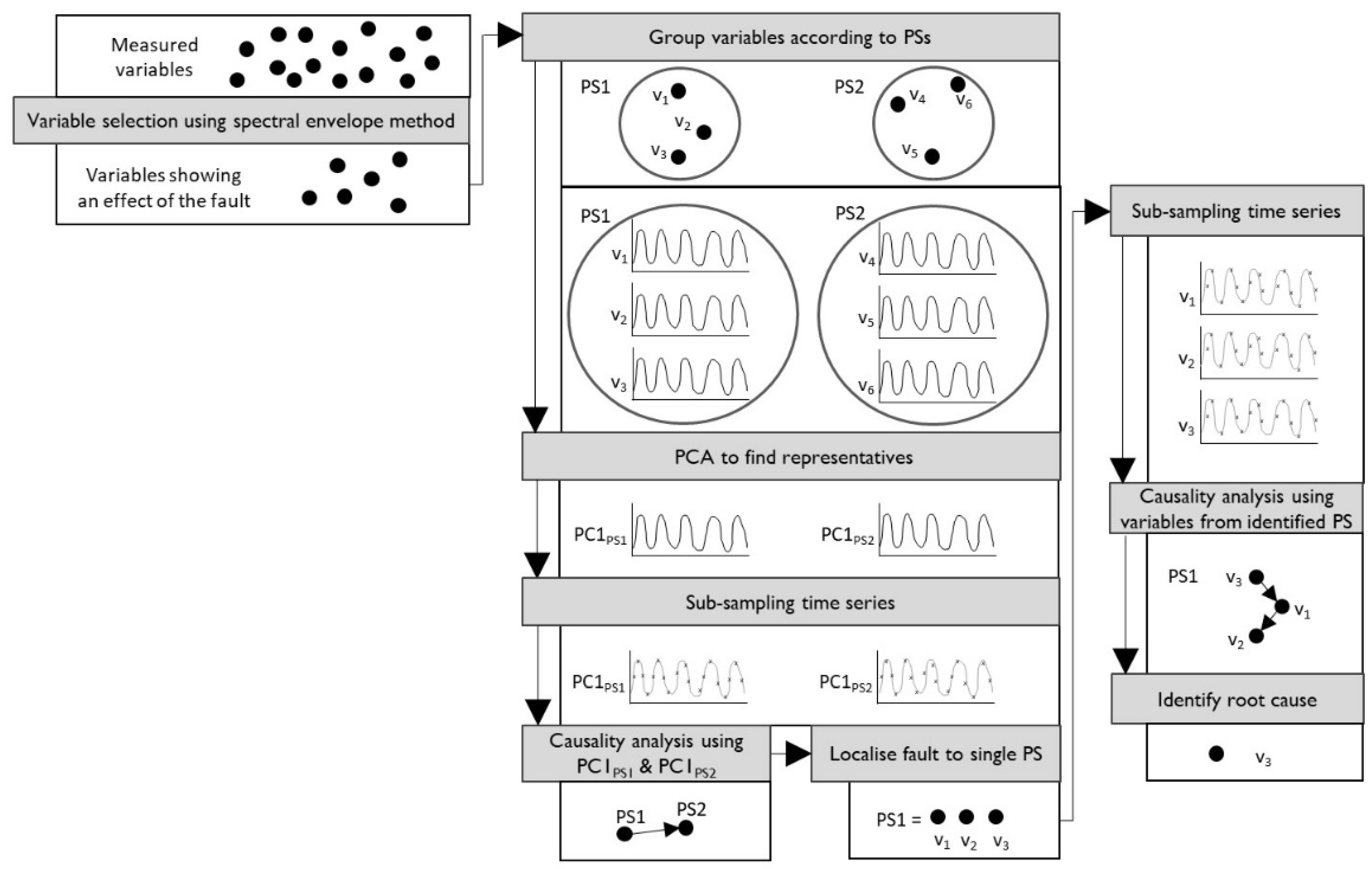
The hierarchical approach for plant-wide causality analysis, termed PS-PC1, uses PCA [37] and cGC to produce causality maps in two subsequent stages, with the workflow depicted in Figure 1. In the first stage, a dimensionally reduced, plant-wide map is constructed and used to localise the root cause to a specific PS; followed by the second stage, where a causality map is constructed for only that PS and used to identify the root cause.
Stage one in the hierarchical approach starts after variable selection (discussed in Section 2.2) was applied to identify all variables showing an effect of the fault. The first step is grouping these variables according to PSs, followed by applying dimensionality reduction via PCA to find representatives for each PS, and performing data selection (discussed in Section 2.2) on the representative time series of each PS. Thereafter, cGC is performed using the sub-sampled, representative time series of the PSs to construct a dimensionally reduced, plant-wide causality map, where each node represents a PS. The representative of each PS is taken as the first principal component (PC1) of that PS, so that the root cause can be traced to a single node representing a single PS in the plant-wide causality map.
2.4. Benchmarking the Hierarchical Approach
The novel hierarchical approach was benchmarked by comparison to (1) the causality map constructed from application of cGC using all measured variables in the plant that show an effect of the fault, termed the standard causality map in this work, and (2) the transitive reduction of the standard causality map.
The transitive reduction of a causality map is a pruned version of the causality map, where shortcut connections (i.e., causal connections due to the influence of an intermediate variable) are identified and removed using a depth-first search algorithm [38]. The transitive reduction of causality map G is another map Greduction with the same number of nodes, but with the fewest edges that still allow Greduction to have the same reachability (i.e., ability to travel from one node to another within the map) [38]—meaning that the transitive reduction of a causality map retains all the propagation paths but with fewer edges.
3. Results and Discussion
The novel hierarchical approach was applied to a simulated tank network. The aim of the simulation is to serve as a case study which, although artificial, clearly demonstrates the smearing effect. While the case study is intentionally designed to challenge causality analysis algorithms, the conceptual simplicity of the system ensures that the ground truth is easily determined by humans, enabling a critical evaluation of the proposed methods. This section therefore provides a process description of the tank network, the fault to be identified using causality analysis, and the results from applying the hierarchical approach to the case study, with comparison to the standard causality map and its transitive reduction.
3.1. Process Description
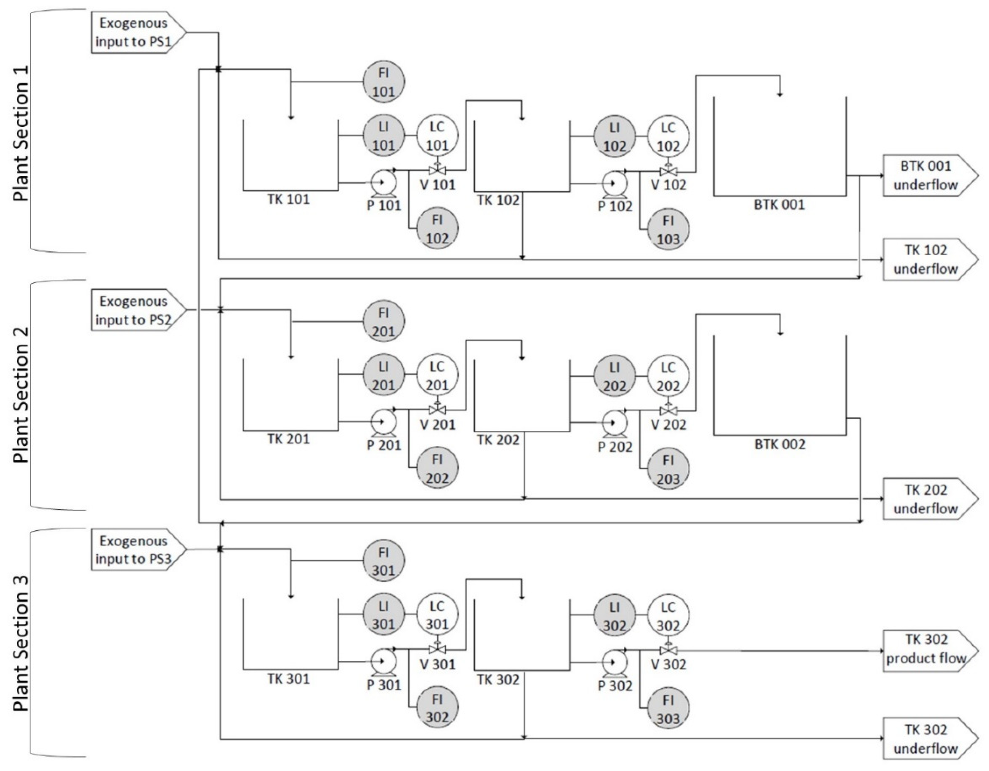
The tank network consists of multiple tanks with liquid inventory, as shown in the diagram provided in Figure 2. The tank network was developed to represent a plant with three PSs that have identical configurations and are separated by buffer tanks (BTK 001 and BTK 002). A detailed description of PS1 is therefore provided, followed by a description of the interaction between the PSs. In addition, the one-tank model development is provided as supplementary material, where Figure S1 provides a diagram with symbols corresponding to the one-tank model and Figure S2 depicts the Simulink implementation of the model.
PS1 consists of two tanks in series (TK 101 and TK 102), with an exogenous input fed to the first tank (TK 101). The exogenous input is modelled as an AR model with the slope parameter equal to one, as shown in Figure S3 in the supplementary material, to simulate real-world disturbances which are not entirely time independent. Both tanks have a constant product flow through a throttled centrifugal pump that leads to the next tank in series. The second tank (TK 102) also has a level-dependent underflow, of which 50% is recycled back to the first tank (TK 101) and the rest is purged.
The buffer tanks (BTK 001 and BTK 002) are used to attenuate disturbances between PSs, and both have a level-dependent underflow of which 65% is fed to the next PS. The rest of the underflow from BTK 001 is purged, but the rest of the underflow from BTK 002 is recycled back to TK 101 in PS1 to increase the interconnectivity between PSs. Dead times of 5 and 10 min are artificially present in the pipes within and between PSs, respectively, to incorporate the phenomena of time delay that is typically present in industrial mineral processing plants.
Downstream inventory control is implemented on all the tanks within PSs (i.e., excluding buffer tanks). The controlled variables are the levels and the manipulated variables are the throttling valves on the product lines. Linear averaging level control is implemented to maintain the controlled variables at their set points of 0.5 (i.e., half full tanks) with an allowable deviation of 10%.
3.2. Process Fault
Valve stiction was incorporated as the fault in the tank network simulation. It is a commonly occurring fault known to cause plant-wide oscillations, so it successfully demonstrates the smearing effect in the simulation. For this study, the dynamics of valve stiction were simulated using an empirical model [39], where the valve becomes stuck every time it attempts to change direction and subsequently remains stuck while Equations (6) and (7) remain true:
where L(k) is the controller output for valve position, Lss is the current stuck valve position, and the two parameters J (slipjump) and S (deadband + stickband) were set to 60% and 65%, respectively.
The valve stiction is present in the second control valve in PS2 (V-202 in Figure 2), meaning that the fault needs to propagate both downstream and upstream to reach all variables in the plant. This incorporates the recycle stream from PS2 to PS1 in the fault propagation path, which represents the interconnectivity and often cyclic interaction present in mineral processing plants.
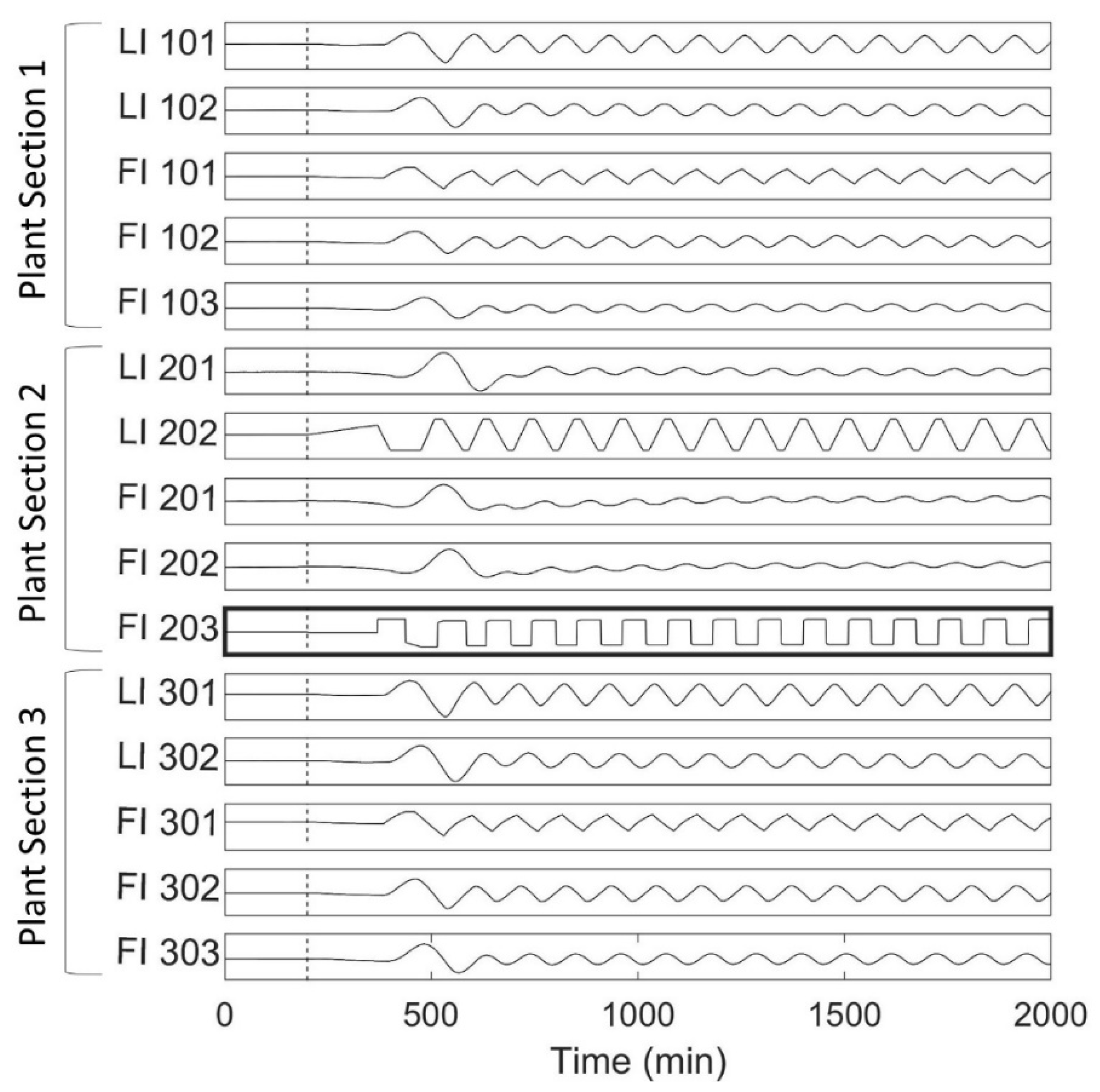
The time series for all 15 measured variables are presented in Figure 3, where PSs are indicated by open brackets on the left-hand side and the first number in each tag name indicates its PS. The valve stiction begins at 200 min, as indicated by the dashed line in Figure 3. The first effect of the fault is seen as a small dip in the flowrate being adjusted by the sticky valve (FI 203), which almost immediately affects its controlled variable (LI 202), after which the fault propagates as an oscillation to all the other measured variables.
3.3. Variable Selection, Data Selection and Dimensionality Reduction
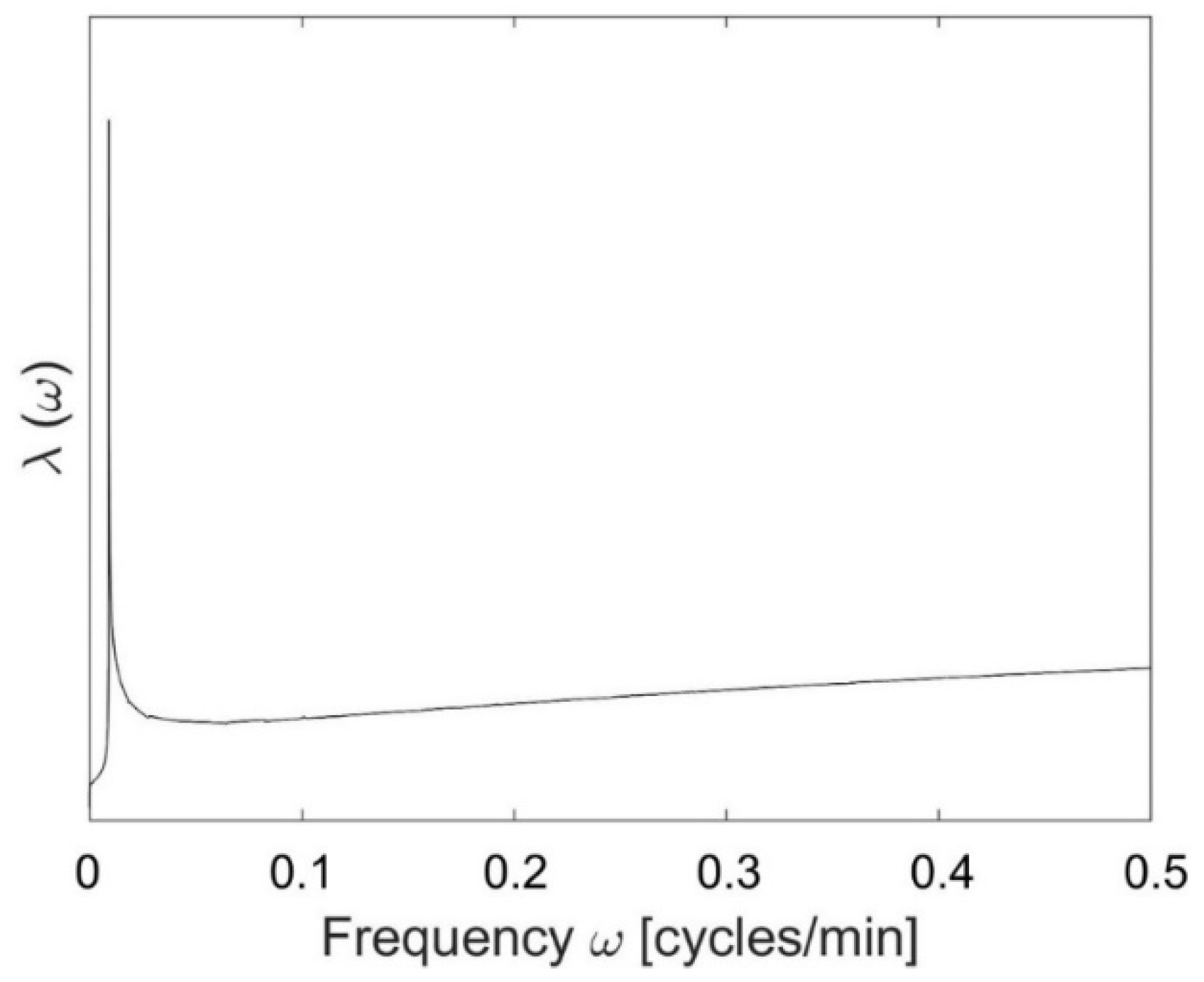
Variables showing an effect of the fault were identified and selected as those with a common oscillation frequency (discussed in Section 2.2). A common oscillation frequency was identified at 0.0091 cycles·min-1 from the spectral envelope plot in Figure 4, obtained for the fault-state data (i.e., from after the dotted line in Figure 3). This corresponds to a period of 110 min, which matches the period of oscillation observed in the time series where the valve stiction occurs (FI 203 in Figure 3). All the measured variables were found to oscillate significantly at the common oscillation frequency (with p-values associated with the test statistic of larger than 0.999), so all measured variables were selected to include in causality analysis.
Prior to each causality analysis calculation, data selection was performed by selecting a SP and TW to pre-process the time series data (as discussed in Section 2.2). For the standard map, the G-causality index (defined in Equation (3)) for the known connection FI 203 LI 202 (level control loop; see Figure 2) was calculated for the SP range 1–27 min (where 27 min was the maximum SP where the data maintained an acceptable resolution) and the corresponding TWs (as discussed in Section 2.2). The largest G-causality index for FI 203 LI 202 was obtained using the data pre-processed with an SP of 27 min and a TW of 38 days, so this dataset was used to produce the standard causality map.
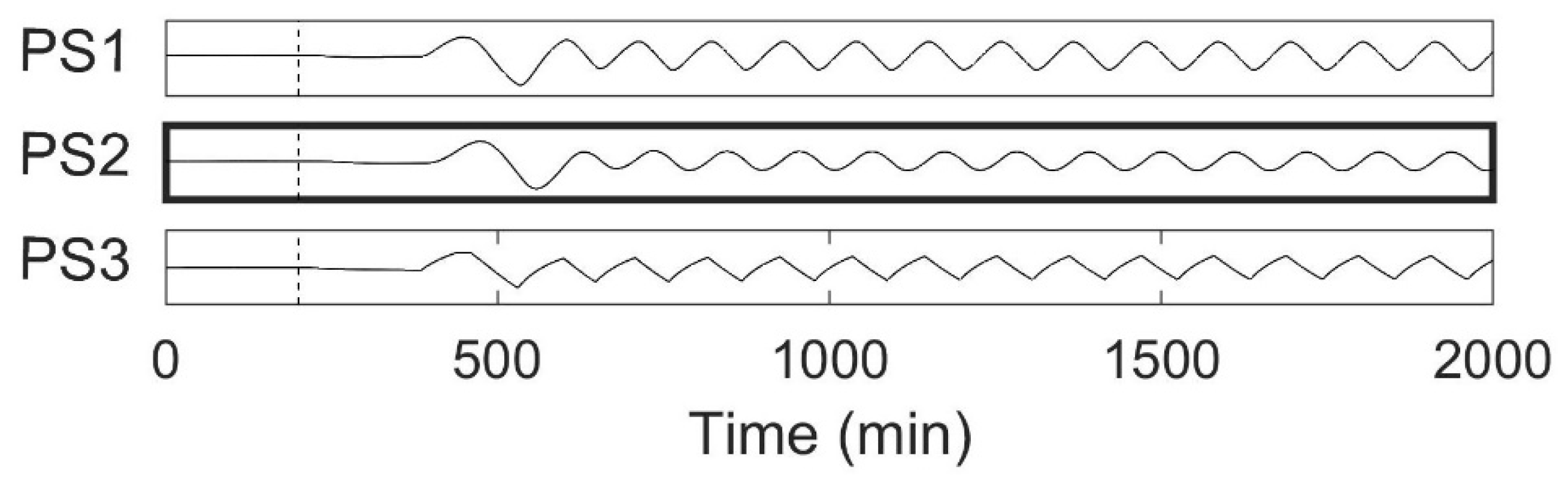
For the PS-PC1 plant-wide map, data selection was performed on the representative (PC1) time series for each PS, shown in Figure 5. The G-causality index was calculated for the known connection PS2 PS1 (due to the recycle stream between the PSs; see the process diagram in Figure 2) for the SP range 1–7 min (where 7 min was the maximum SP where the data maintained acceptable resolution) and the corresponding TWs (discussed in Section 2.2). The largest G-causality index value for this connection was obtained when the dimensionally reduced data was pre-processed using a SP and TW of 5 min and 2.1 days, respectively, and this dataset was used to produce the PS-PC1 plant-wide map. For the PS-PC1 PS map, the G-causality index for the connection FI 203 LI 202 (a known connection within PS2, where the fault is localised to in stage one of the hierarchical approach; see Section 3.4) was calculated for the SP range 1–27 min and corresponding TWs; the largest value was obtained for a SP of 25 min and TW of 14.1 days; that dataset was used to produce the PS-PC1 PS map.
The approaches for all three cases were validated by inspecting the resulting time frame (after model order selection had occurred using AIC) for each combination of SP and TW and comparing it to the expected temporal relationship between the variables in the selected, known connection. Any combination of SP and TW that resulted in a significant difference between the obtained and expected time frame was excluded from further consideration. In this work, the expected time frame was determined using a step test, which may not always be possible in industry. In an industrial application, the plant operator or engineer can use their process knowledge to estimate low and high cut-off points for the expected time frame that should be captured in the known causal connection.
3.4. Causality Maps
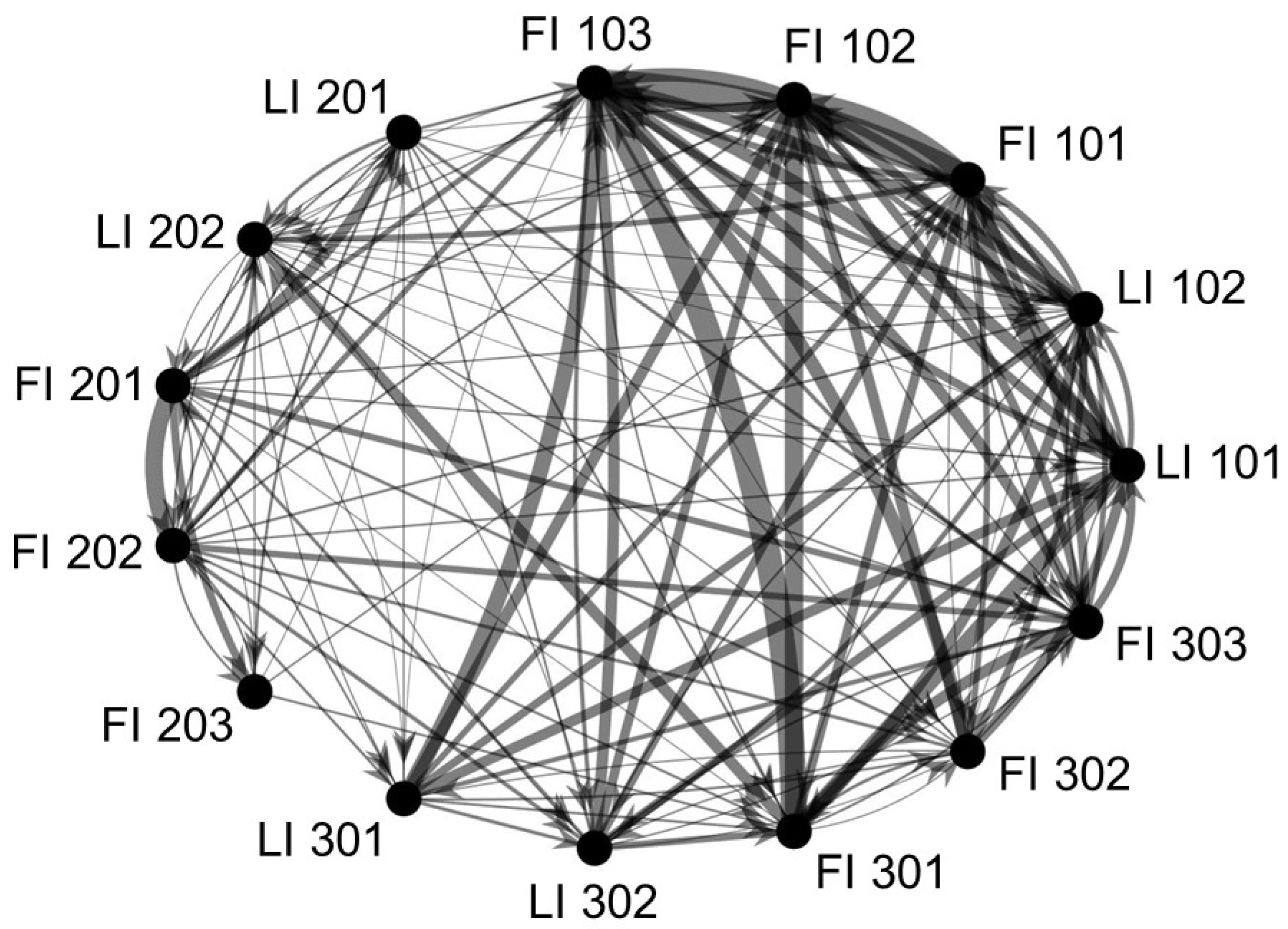
The standard causality map to identify the fault in the tank network case study is provided in Figure 6. The purpose of a causality map in fault identification is to identify the fault location by allowing the propagation path to be traced back to its root cause. If the causality map is acyclic, the root cause is easily identifiable, but due to the many cyclic interactions in control loops and recycle streams, that is not the case in this study and often not in industrial mineral processing plants.
Since the causality map is cyclic, the root cause is typically identified by finding a node on the causality map that is shown to have a large causal influence—which has a subjective meaning, but can generally be taken to mean that the node has the most or many directed edges pointing from it to other nodes and/or the node has strong connections (i.e., heavily weighted edges indicating strong causal connections) adjacent to it. However, there is no node or group of nodes (e.g., nodes belonging to the same process unit or PS that can be further investigated) that can clearly be seen to have a large causal influence in this standard causality map (Figure 6). An argument could potentially be made that most of the heavier edges originate or end at nodes representing variables in PS1 or PS3, but not only is that interpretation insufficient and incorrect, it is subjective and would likely differ from person to person.
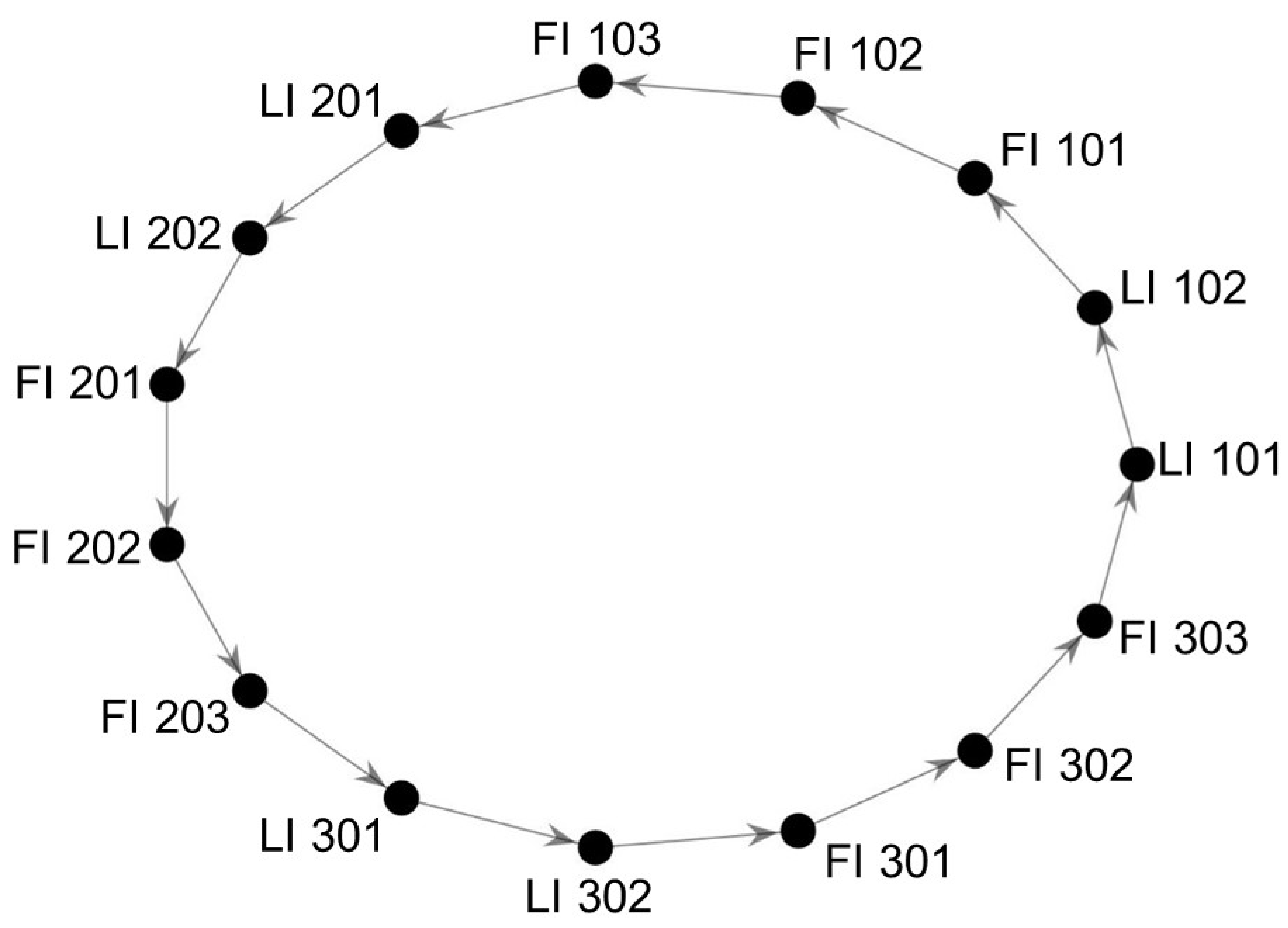
One reason for the difficulty in interpreting the standard causality map (Figure 6) is its density. The transitive reduction of the standard map is therefore provided in Figure 7, where all shortcut edges have been removed (as explained in Section 2.4). However, this map is completely cyclic and has no edge weights (since causal strengths are not considered in a transitive reduction), making it impossible to identify the root cause of the fault using this map.
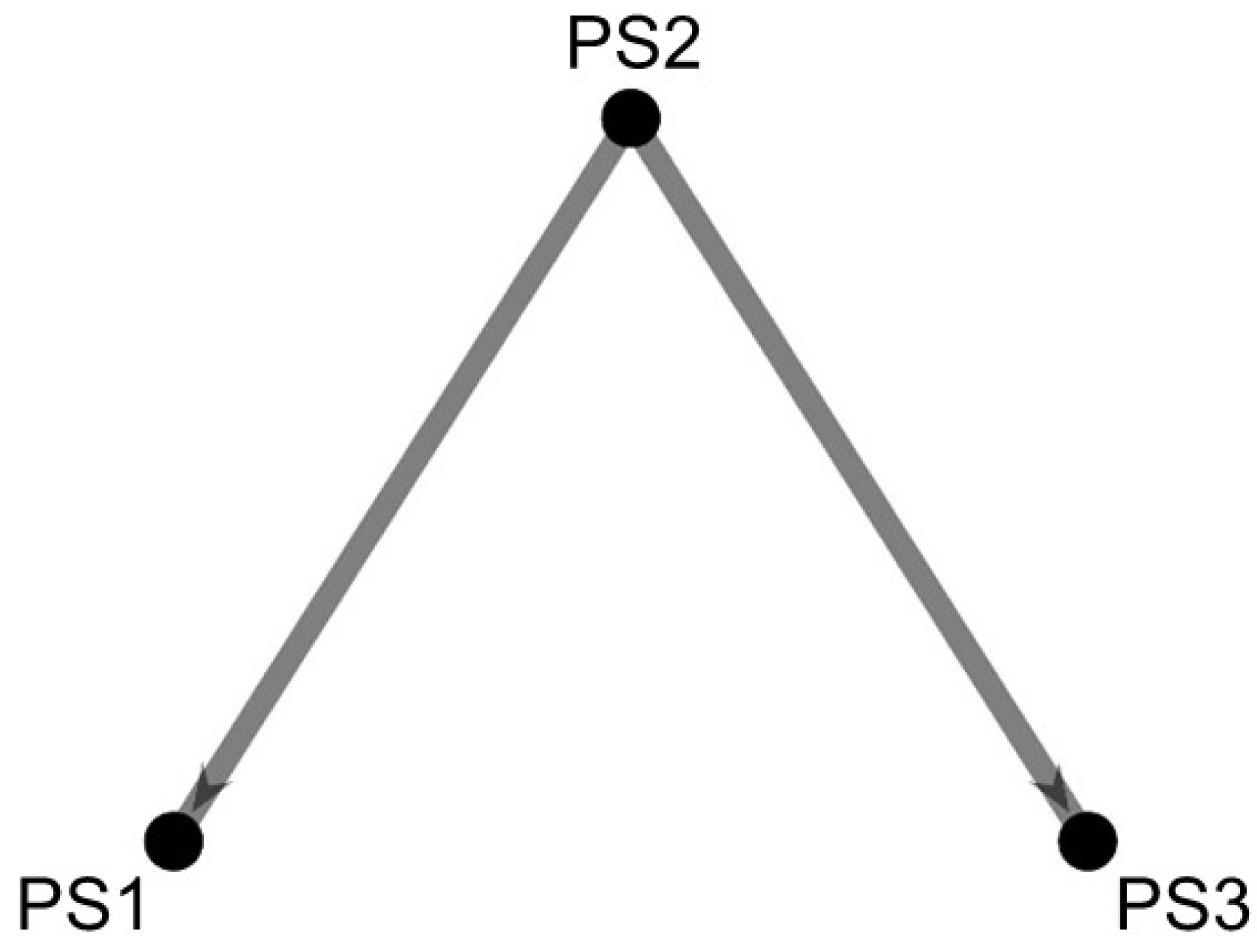
The hierarchical approach, PS-PC1, consists of two sequential causality maps, where the first one is the PS-PC1 plant-wide map provided in Figure 8. This plant-wide map (Figure 8) is acyclic, with no edges pointing towards PS2, and two heavy edges pointing from PS2 to PS1 and PS3, respectively. It is therefore clear that PS2 is identified as the root cause location.
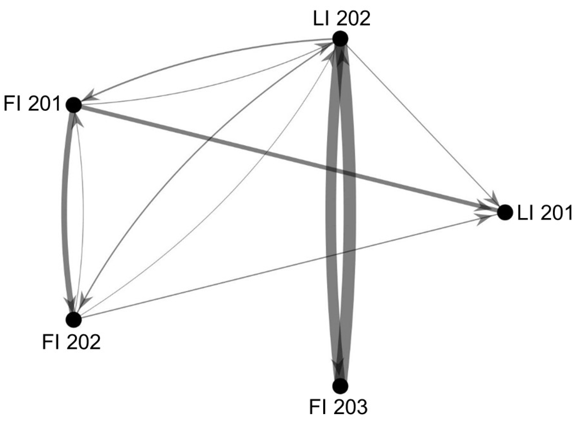
The second map in the hierarchical approach, the PS-PC1 PS map (Figure 9), therefore consists of all variables in PS2 that show an effect of the fault. This causality map is also cyclic, so the root cause should be identified as a node with a large causal influence, which can be identified by observing the nodes adjacent to heavier edges (i.e., strong causal connections, large value of G-causality index defined in Equation (3) in Section 2.1)–FI 201, LI 202, FI 203 and LI 201. These nodes can then each be considered as the potential root cause. The most obvious candidate to exclude is LI 201 since no edge weights originate at this node, which makes it unlikely to be the root cause.
Process knowledge (e.g., gained from a process schematic like Figure 2) can then be used to identify the root cause from the remaining options. FI 203 and LI 202 are considered together since they constitute one control loop. This control loop is shown with heavy edges (i.e., strong causal connections), which is notably different from the other control loop, FI 202 and LI 201 (which is more upstream), that is shown with light edges. Furthermore, the only other node in question, FI 201, is upstream from all the other variables, which makes it likely that it only has a large effect on the causal structure because of its position in the process structure. FI 203 and LI 202 are therefore distinct as they are downstream from the other variables, but are still shown with heavy edges (i.e., strong causal connections in the presence of the current fault), which indicates that they are likely associated with the root cause (which is true).
The hierarchical approach, PS-PC1 is therefore benchmarked against the standard causality map and the transitive reduction of the standard causality map. Neither the standard causality map nor the transitive reduction could be interpreted to clearly identify the true root cause; while the PS-PC1 plant-wide map could be clearly interpreted to localise the fault to PS2, and the PS-PC1 PS map of PS2 clearly interpreted to identify the control loop consisting of FI 203 and LI 202 as the root cause (which is correct, as the true root cause is a faulty valve on line FI 203). In this case, the PS-PC1 plant-wide map was acyclic, making fault identification clear and simple. Furthermore, the two causality maps in the hierarchical approach consisted of only three and five nodes, respectively, compared to the 15 nodes in the standard causality map and the transitive reduction. The PS-PC1 plant-wide map has nodes equal to the number of PSs that contain at least one variable showing an effect of the fault, and the PS-PC1 PS map has nodes equal to the number of variables in that PS that show an effect of the fault. The maximum number of nodes in the PS-PC1 plant-wide map is therefore equal to the number of PSs and the maximum number of nodes in the PS-PC1 PS map is equal to the number of variables in that PS—which will both be consistently fewer than the number of nodes in the standard causality map and the transitive reduction, where the number of nodes equals the number of measured variables in the plant showing an effect of the fault. This decreased number of nodes and the resulting simplification of the causality map is the main advantage of the hierarchical approach, and what prepares causality analysis for use in industrial mineral processing plants, where there are significantly more measured variables than in the tank network considered in this study.
3.5. Fault-State Data Requirements
In addition to the improved interpretability of the causality maps, the hierarchical approach also requires significantly less fault-state data than the standard causality map or the transitive reduction. As described in Section 2.1, cGC involves fitting a full AR model that predicts all variables as a function of the past values of all other variables (and each variable at each point in time requires an individual coefficient). For the causality analysis results to be meaningful, that full model needs to have a unique OLS regression solution, which means that there must be more fault-state data points available than required parameters. The hierarchical approach includes fewer variables in each causality analysis calculation, which means fewer parameters are required for the full model, which, in turn, means fewer data points are required for a unique OLS solution of the full model.
The amount of fault-state data required by the hierarchical approach depends on whether there are more PSs in the plant (in which case PS-PC1 plant-wide map has more nodes and requires more data) or more variables in the PS that the fault is localised to in the first stage of the approach (in which case PS-PC1 PS map has more nodes and requires more data). However, Table 2 shows that both the PS-PC1 plant-wide map and the PS-PC1 PS map require fault-state data in the order of hours or days, while the standard map (and therefore also the transitive reduction) requires fault-state data in the order of weeks or months, which defeats the purpose of identifying the root cause of a fault as quickly as possible.
3.6. Limitations
The hierarchical approach for causality analysis, PS-PC1, presented in this work shows promising results, but its limitations should be noted. As with all causality analysis techniques, the variables present in causality maps are limited to measured variables in the process, and the true root cause of the fault may not always be associated with a measured variable. For example, if the root cause of a fault is impeller wear, the closest a causality map could come to identifying the root cause is by pointing to a flow or pressure indicator near the impaired pump. Based on that result, the pump and potentially adjacent unit processes would then need to be further investigated to identify impeller wear as the true root cause.
Another limitation lies with the data selection in the PS-PC1 workflow. The robustness of the heuristic approach for selecting SP and TW used in the PS-PC1 workflow has not been tested, as that was not the aim of this study. In this heuristic approach, SP and TW are selected based on the G-causality index of a chosen known causal connection. In this study, the known connection for both the plant-wide and PS maps were connections associated with the true root cause location (PS2) and true root cause (FI 203/LI 202 control loop), respectively. In industry the true root cause is not known a priori, so a different known connection will likely be used to base this pre-processing SP and TW selection off. Since different causal connections operate at different time scales (due to differences in residence times, controller dynamics, etc.), the selected known connection could be highlighted at a time scale (and the associated SP and TW combination) that does not highlight the true root cause, so obscuring the root cause. However, it should be noted that the PS-PC1 workflow is not dependent on this heuristic approach to select SP and TW; it was used because no alternative was available in literature. Future applications of the PS-PC1 approach could use a different method for SP and TW selection if one becomes available.
Lastly, the PS-PC1 plant-wide map relies on a single PC to capture sufficient variance to represent an entire PS. In the mineral processing industry, PSs can consist of hundreds of variables compared to the five variables per PS present in this study, so one PC may fail to accurately represent an entire PS.
4. Conclusions
The novel hierarchical approach presented in this work is the required next step in literature to prepare causality analysis for application in the mineral processing industry. It builds upon the previous research on causality analysis that focussed on improving the techniques such as cGC themselves and addresses the need for improved interpretability of causality maps, which becomes more vital as the system being analysed increases in scale. This work takes causality analysis from being applicable to only a few variables and presents it as a usable method for plant-wide fault identification.
The approach is benchmarked against the standard causality map and its transitive reduction and shown to improve causality map interpretability. The causality maps in the hierarchical approach could be interpreted to identify the true root cause, while consisting of three and five nodes, respectively, compared to the 15 nodes in the standard map and the transitive reduction. Furthermore, this novel approach addresses the practicality of fault-state data requirements for cGC, requiring data in the order of hours or days instead of weeks or months. This is especially relevant in industry, where a fault should be identified in a timely fashion.
Limitations to the approach include the fact that variables in the causality maps are limited to measured process variables; a current lack of testing of the robustness of the heuristic approach used for SP and TW selection during data pre-processing; the reliance on a single PC to represent an entire PS in the plant-wide map.
Future work will apply this approach to an industrial dataset to determine whether sufficient data can be captured in PC1 to represent a PS that contains numerous measured variables. Such work could consider increasing the number of stages in the hierarchical approach beyond two or decreasing the number of variables per PS by only using manipulated variables or only using controlled variables.
Alternatively, a future research direction could be to investigate whether multivariate Granger causality [31,40] can be used instead of PCA and pairwise cGC in the first stage of the hierarchical approach, where causal interactions between groups of variables compromising each PS are considered. However, a limitation to this approach would be that it would require as much fault-state data as standard cGC, as there is no dimensionality reduction involved.
Supplementary Materials
The following are available online at https://www.mdpi.com/article/10.3390/min11080823/s1, Figure S1: Diagram with symbols corresponding to one-tank model, Figure S2: Simulink implementation of the one-tank model, Figure S3: Random walk implementation in Simulink.
Author Contributions
Conceptualisation, L.A. and N.v.Z.; methodology, N.v.Z., T.M.L., S.M.B. and L.A.; software, N.v.Z.; validation, N.v.Z.; formal analysis, N.v.Z.; writing—original draft preparation, N.v.Z.; writing—review and editing, N.v.Z., T.M.L. and S.M.B.; visualisation, N.v.Z.; supervision, T.M.L., S.M.B. and L.A.; project administration, T.M.L. and S.M.B.; funding acquisition, L.A. All authors have read and agreed to the published version of the manuscript.
Funding
This research was funded by Anglo American Platinum, grant number S005963RES01.
Data Availability Statement
Not applicable.
Conflicts of Interest
The authors declare no conflict of interest.
Nomenclature
| Symbols | |
| C | Coefficient |
| F | F-statistic |
| G-causality index | |
| J | Slipjump |
| L | Controller output for valve position |
| Lss | Current stuck valve position |
| N | Number of observations |
| N | Number of variables |
| p | Model order |
| S | Deadband + stickband |
| V | Valve |
| V | Variable |
| Greek symbols | |
| Residual error | |
| Spectral envelope | |
| Residual covariance matrix | |
| Frequency | |
| Subscripts and superscripts | |
| Full | Full model |
| Res | Restricted model |
| Abbreviations and acronyms | |
| AIC | Akaike information criterion |
| ANN | Artificial neural network |
| AR | Autoregressive |
| BTK | Buffer tank |
| cGC | Conditional Granger causality |
| FI | Flow indicator |
| LC | Level controller |
| LI | Level indicator |
| OLS | Ordinary least squares |
| P | Pump |
| PCA | Principle component analysis |
| PC | Principal component |
| PS | Plant section |
| PS-PC1 | Hierarchical approach for plant-wide causality analysis presented in this paper |
| SP | Sampling period |
| TK | Tank |
| TW | Time window |
References
- Reis, M.; Gins, G. Industrial process monitoring in the big data/industry 4.0 era: From detection, to diagnosis, to prognosis. Processes 2017, 5, 35. [Google Scholar] [CrossRef] [Green Version]
- Jemwa, G.T.; Aldrich, C. Kernel-Based fault diagnosis on mineral processing plants. Miner. Eng. 2006, 19, 1149–1162. [Google Scholar] [CrossRef]
- Wakefield, B.J.; Lindner, B.S.; McCoy, J.T.; Auret, L. Monitoring of a simulated milling circuit: Fault diagnosis and economic impact. Miner. Eng. 2018, 120, 132–151. [Google Scholar] [CrossRef]
- Krishnannair, S.; Aldrich, C. Process monitoring and fault detection using empirical mode decomposition and singular spectrum analysis. IFAC Pap.-OnLine 2019, 52, 219–224. [Google Scholar] [CrossRef]
- Zhang, C.; Peng, K.; Dong, J. An incipient fault detection and self-learning identification method based on robust SVDD and RBM-PNN. J. Process Control 2020, 85, 173–183. [Google Scholar] [CrossRef]
- Van den Kerkhof, P.; Vanlaer, J.; Gins, G.; Van Impe, J.F.M. Analysis of Smearing-out in contribution plot based fault isolation for statistical process control. Chem. Eng. Sci. 2013, 104, 285–293. [Google Scholar] [CrossRef]
- Miller, P.; Swanson, R.E.; Heckler, C.E. Contribution plots: A missing link in multivariate quality control. AMCS 1998, 8, 775–792. [Google Scholar]
- Westerhuis, J.A.; Gurden, S.P.; Smilde, A.K. Generalized contribution plots in multivariate statistical process monitoring. Chemom. Intell. Lab. Syst. 2000, 51, 95–114. [Google Scholar] [CrossRef]
- Perez, L.G.; Flechsig, A.J.; Meador, J.L.; Obradovic, Z. Training an artificial neural network to discriminate between magnetizing inrush and internal faults. IEEE Trans. Power Deliv. 1994, 9, 434–441. [Google Scholar] [CrossRef]
- Moravej, Z. Evolving neural nets for protection and condition monitoring of power transformer. Electr. Mach. Power Syst. 2005, 33, 1229–1236. [Google Scholar] [CrossRef]
- Sun, W.; Paiva, A.R.C.; Xu, P.; Sundaram, A.; Braatz, R.D. Fault detection and identification using bayesian recurrent neural networks. Comput. Chem. Eng. 2020, 141, 106991. [Google Scholar] [CrossRef]
- Khoukhi, A.; Khalid, M.H. Hybrid computing techniques for fault detection and isolation, a review. Comput. Electr. Eng. 2015, 43, 17–32. [Google Scholar] [CrossRef]
- Li, W.; Peng, M.; Wang, Q. Fault identification in PCA method during sensor condition monitoring in a nuclear power plant. Ann. Nucl. Energy 2018, 121, 135–145. [Google Scholar] [CrossRef]
- Sánchez-Fernández, A.; Sainz-Palmero, G.I.; Benítez, J.M.; Fuente, M.J. Linguistic OWA and two time-windows based fault identification in wide plants. Comput. Chem. Eng. 2018, 115, 412–430. [Google Scholar] [CrossRef]
- Lindner, B.; Auret, L.; Bauer, M. Investigating the impact of perturbations in chemical processes on data-based causality analysis. Part 1: Defining desired performance of causality analysis techniques * *the authors gratefully acknowledge anglo american platinum for the financial support that made this research possible. IFAC Pap.-OnLine 2017, 50, 3269–3274. [Google Scholar] [CrossRef]
- Groenewald, J.W.D.; Aldrich, C. Root cause analysis of process fault conditions on an industrial concentrator circuit by use of causality maps and extreme learning machines. Miner. Eng. 2015, 74, 30–40. [Google Scholar] [CrossRef]
- Esquivel, A.E. Capturing and Exploiting Plant Topology and Process Information as a Basis to Support Engineering and Operational Activities in Process Plants. Ph.D. Dissertation, Helmit Schmidt University, Hamburg, Germany, 2017. [Google Scholar]
- Yim, S.Y.; Ananthakumar, H.G.; Benabbas, L.; Horch, A.; Drath, R.; Thornhill, N.F. Using process topology in plant-wide control loop performance assessment. Comput. Chem. Eng. 2006, 31, 86–99. [Google Scholar] [CrossRef] [Green Version]
- Thambirajah, J.; Benabbas, L.; Bauer, M.; Thornhill, N.F. Cause-and-effect analysis in chemical processes utilizing XML, plant connectivity and quantitative process history. Comput. Chem. Eng. 2009, 33, 503–512. [Google Scholar] [CrossRef] [Green Version]
- Yang, F.; Duan, P.; Shah, S.L.; Chen, T. Capturing Connectivity and Causality in Complex, Industrial Processes, 1st ed.; Springer Briefs in Applied Sciences and Technology; Springer: Cham, Germany, 2014; ISBN 978-3-319-05380-6. [Google Scholar]
- Granger, C.W.J.; Newbold, P. Spurious regressions in econometrics. J. Econom. 1974, 2, 111–120. [Google Scholar] [CrossRef] [Green Version]
- Geweke, J. Measurement of linear dependence and feedback between multiple time series. J. Am. Stat. Assoc. 1982, 77, 304–313. [Google Scholar] [CrossRef]
- Lindner, B.; Chioua, M.; Groenewald, J.W.D.; Auret, L.; Bauer, M. Diagnosis of oscillations in an industrial mineral process using transfer entropy and nonlinearity index. IFAC Pap.-OnLine 2018, 51, 1409–1416. [Google Scholar] [CrossRef]
- Duan, P.; Chen, T.; Shah, S.L.; Yang, F. Methods for root cause diagnosis of plant-wide oscillations. AIChE J. 2014, 60, 2019–2034. [Google Scholar] [CrossRef]
- Lindner, B.S. Improving the Performance of Causality Analysis Techniques for Automated Fault Diagnosis in Mineral Processing Plants. PhD Dissertation, University of Stellenbosch, Stellenbosch, South Africa, 2019. [Google Scholar]
- Suresh, R.; Sivaram, A.; Venkatasubramanian, V. A hierarchical approach for causal modeling of process systems. Comput. Chem. Eng. 2019, 123, 170–183. [Google Scholar] [CrossRef]
- Liu, Y.; Chen, H.-S.; Wu, H.; Dai, Y.; Yao, Y.; Yan, Z. Simplified granger causality map for data-driven root cause diagnosis of process disturbances. J. Process Control 2020, 95, 45–54. [Google Scholar] [CrossRef]
- Lindner, B.; AUret, L. Application of data-based process topology and feature extraction for fault diagnosis of an industrial platinum group metals concentrator plant. IFAC Pap.-Online 2015, 48, 102–107. [Google Scholar] [CrossRef]
- Yuan, T.; Qin, S.J. Root cause diagnosis of plant-wide oscillations using granger causality. J. Process Control 2014, 24, 450–459. [Google Scholar] [CrossRef]
- MATLAB; The MathWorks Inc.: Natick, MA, USA, 2018.
- Geweke, J.F. Measures of conditional linear dependence and feedback between time series. J. Am. Stat. Assoc. 1984, 79, 907–915. [Google Scholar] [CrossRef]
- Barnett, L.; Seth, A.K. The MVGC multivariate granger causality toolbox: A new approach to granger-causal inference. J. Neurosci. Methods 2014, 223, 50–68. [Google Scholar] [CrossRef] [Green Version]
- Hill, R.C.; Griffiths, W.E.; Lim, G.C. Principles of Econometrics, 4th ed.; John Wiley & Sons, Inc.: Hoboken, NJ, USA, 2011; ISBN 978-0-470-62673-3. [Google Scholar]
- Hurvich, C.M.; Tsai, C.-L. Regression and time series model selection in small samples. Biometrika 1989, 76, 297–307. [Google Scholar] [CrossRef]
- Bressler, S.L.; Seth, A.K. Wiener–granger causality: A well established methodology. NeuroImage 2011, 58, 323–329. [Google Scholar] [CrossRef] [PubMed]
- Jiang, H.; Choudhury, S.M.A.A.; Shah, S.L. Detection and diagnosis of plant-wide oscillations from industrial data using the spectral envelope method. J. Process Control 2007, 17, 143–155. [Google Scholar] [CrossRef]
- Abdi, H.; Williams, L.J. Principal component analysis. WIREs Comp. Stat. 2010, 2, 433–459. [Google Scholar] [CrossRef]
- Aho, A.V.; Garey, M.R.; Ullman, J.D. The transitive reduction of a directed graph. SIAM J. Comput. 1972, 1, 131–137. [Google Scholar] [CrossRef] [Green Version]
- Choudhury, S.M.A.A.; Thornhill, N.F.; Shah, S.L. Modelling valve stiction. Control. Eng. Pract. 2005, 13, 641–658. [Google Scholar] [CrossRef] [Green Version]
- Barrett, A.B.; Barnett, L.; Seth, A.K. Multivariate granger causality and generalized variance. Phys. Rev. E 2010, 81. [Google Scholar] [CrossRef] [Green Version]
Figure 1.
Flow diagram of the hierarchical approach, PS-PC1, with variable selection on the left, Stage 1 in the middle, and Stage 2 on the right. PS, plant section; PC, principal component; v, variable.
Figure 1.
Flow diagram of the hierarchical approach, PS-PC1, with variable selection on the left, Stage 1 in the middle, and Stage 2 on the right. PS, plant section; PC, principal component; v, variable.

Figure 2.
Diagram of tank network consisting of three PSs. PSs are indicated by open brackets on the left-hand side and the first number in each tag name indicates its PS. Shaded sensors indicate measured variables. LI, level indicator; FI, flow indicator; LC, level controller; V, valve; P, pump; TK, tank; BTK, buffer tank.

Figure 3.
Time series data generated using tank network simulation with and without valve stiction online FI 203 (indicated with a bold border). The vertical dashed line indicates the beginning of the valve stiction. PSs are indicated by open brackets on the left-hand side and the first number in each tag name indicates its PS. LI, level indicator; FI, flow indicator.

Figure 4.
Spectral envelope plot of the fault-state time series data obtained from the tank network simulation. , frequency; , spectral envelope.
Figure 4.
Spectral envelope plot of the fault-state time series data obtained from the tank network simulation. , frequency; , spectral envelope.

Figure 5.
Time series for the first principal component of each PS with and without valve stiction on line FI 203 located in PS2 (indicated with a bold border). The vertical dashed line indicates the beginning of the valve stiction.
Figure 5.
Time series for the first principal component of each PS with and without valve stiction on line FI 203 located in PS2 (indicated with a bold border). The vertical dashed line indicates the beginning of the valve stiction.

Figure 6.
Standard causality map to identify the fault in the tank network. The true root cause is a faulty valve on line FI 203. Edge weights represent magnitude of causal influence (measured by the G-causality index defined in Section 2.1). The first number in each tag name indicates its PS. LI, level indicator; FI, flow indicator.

Figure 7.
Transitive reduction of the standard causality map to identify the fault in the tank network. The true root cause is a faulty valve online FI 203. The first number in each tag name indicates its PS. LI, level indicator; FI, flow indicator.
Figure 7.
Transitive reduction of the standard causality map to identify the fault in the tank network. The true root cause is a faulty valve online FI 203. The first number in each tag name indicates its PS. LI, level indicator; FI, flow indicator.

Figure 8.
PS-PC1 plant-wide causality map, produced in the first stage of the hierarchical approach. The root cause is a faulty valve located in PS2. Edge weights represent magnitude of causal influence (measured by the G-causality index defined in Section 2.1).
Figure 8.
PS-PC1 plant-wide causality map, produced in the first stage of the hierarchical approach. The root cause is a faulty valve located in PS2. Edge weights represent magnitude of causal influence (measured by the G-causality index defined in Section 2.1).

Figure 9.
PS-PC1 PS (PS2) causality map, produced in the second stage of the hierarchical approach. The root cause is a faulty valve located on line FI 203. Edge weights represent magnitude of causal influence (measured by the G-causality index defined in Section 2.1). LI, level indicator; FI, flow indicator.


Table 1.
List of measured variables in simulated tank network case study. The first number in each tag name indicates its PS.
Table 1.
List of measured variables in simulated tank network case study. The first number in each tag name indicates its PS.
| Variable No. | Tag Number | Description | Units |
|---|---|---|---|
| 1 | FI 101 | Total volumetric inlet flowrate to TK 101 | L/min |
| 2 | LI 101 | Level of TK 101 | m/m |
| 3 | FI 102 | Volumetric product flowrate of TK 101 | L/min |
| 4 | LI 102 | Level of TK 102 | m/m |
| 5 | FI 103 | Volumetric product flowrate of TK 102 | L/min |
| 6 | FI 201 | Total volumetric inlet flowrate to TK 201 | L/min |
| 7 | LI 201 | Level of TK 201 | m/m |
| 8 | FI 202 | Volumetric product flowrate of TK 201 | L/min |
| 9 | LI 202 | Level of TK 202 | m/m |
| 10 | FI 203 | Volumetric product flowrate of TK 202 | L/min |
| 11 | FI 301 | Total volumetric inlet flowrate to TK 301 | L/min |
| 12 | LI 301 | Level of TK 301 | m/m |
| 13 | FI 302 | Volumetric product flowrate of TK 301 | L/min |
| 14 | LI 302 | Level of TK 302 | m/m |
| 15 | FI 303 | Volumetric product flowrate of TK 302 | L/min |
Table 2.
Minimum TW of fault-state data required to provide sufficient samples for unique regression solutions. For the standard map/transitive reduction, 13 562 samples are required; for the PS-PC1 plant-wide map, 602 samples are required; for the PS-PC1 PS map, 1562 samples are required.
Table 2.
Minimum TW of fault-state data required to provide sufficient samples for unique regression solutions. For the standard map/transitive reduction, 13 562 samples are required; for the PS-PC1 plant-wide map, 602 samples are required; for the PS-PC1 PS map, 1562 samples are required.
| SP (min) | TW (Days) | ||
|---|---|---|---|
| Standard Map/Transitive Reduction | PS-PC1 Plant-Wide Map | PS-PC1 PS Map | |
| 1 | 9 | 0.4 | 1.1 |
| 2 | 19 | 0.8 | 2.2 |
| 3 | 28 | 1.3 | 3.3 |
| 4 | 38 | 1.7 | 4.3 |
| 5 | 47 | 2.1 | 5.4 |
| 6 | 57 | 2.5 | 6.5 |
| 7 | 66 | 2.9 | 7.6 |
Publisher’s Note: MDPI stays neutral with regard to jurisdictional claims in published maps and institutional affiliations. |
© 2021 by the authors. Licensee MDPI, Basel, Switzerland. This article is an open access article distributed under the terms and conditions of the Creative Commons Attribution (CC BY) license (https://creativecommons.org/licenses/by/4.0/).
Share and Cite
MDPI and ACS Style
van Zijl, N.; Bradshaw, S.M.; Auret, L.; Louw, T.M. A Hierarchical Approach to Improve the Interpretability of Causality Maps for Plant-Wide Fault Identification. Minerals 2021, 11, 823. https://doi.org/10.3390/min11080823
AMA Style
van Zijl N, Bradshaw SM, Auret L, Louw TM. A Hierarchical Approach to Improve the Interpretability of Causality Maps for Plant-Wide Fault Identification. Minerals. 2021; 11(8):823. https://doi.org/10.3390/min11080823
Chicago/Turabian Stylevan Zijl, Natali, Steven Martin Bradshaw, Lidia Auret, and Tobias Muller Louw. 2021. "A Hierarchical Approach to Improve the Interpretability of Causality Maps for Plant-Wide Fault Identification" Minerals 11, no. 8: 823. https://doi.org/10.3390/min11080823
Note that from the first issue of 2016, this journal uses article numbers instead of page numbers. See further details here.