
An Integrated Horizon Picking Method for Obtaining the Main and Detailed Reflectors on Sub-Bottom Profiler Sonar Image


1
School of Geodesy and Geomatics, Wuhan University, Wuhan 430079, China
2
Institute of Marine Science and Technology, Wuhan University, Wuhan 430079, China
3
Department of Artificial Intelligence and Automation, School of Electrical Engineering and Automation, Wuhan University, Wuhan 430072, China
*
Author to whom correspondence should be addressed.
Remote Sens. 2021, 13(15), 2959; https://doi.org/10.3390/rs13152959
Submission received: 21 June 2021
/
Revised: 22 July 2021
/
Accepted: 26 July 2021
/
Published: 28 July 2021
(This article belongs to the Special Issue Near-Surface Geophysics: A Remote Sensing Tool for the Shallow Subsurface)
Abstract
:A sub-bottom profiler (SBP) can capture the sediment interfaces and properties of different types of sediment. Horizon picking from SBP images is one of the most crucial steps in marine sub-bottom sediment interpretation. However, traditional horizon picking methods are good at obtaining the main horizons representing the main reflectors while ignoring the detailed horizons. While detailed horizons are the prime objective, many tiny structures caused by interference echoes will also be picked. To overcome this limitation, an integrated horizon picking method for obtaining the main and detailed horizons simultaneously is proposed in this paper. A total of three main process steps: the diffusion filtering method, the enhancement filtering method as well as the local phase calculation method, are used to help obtain the main and detailed horizons. The diffusion filtering method smooths the SBP images and preserves reflectors. Enhancement filtering can eliminate outliers and enhance reflectors. The local phase can be used to highlight all of the reflections and help in the choosing of detailed horizons. A series of experiments were then performed to validate the effectiveness of the proposed method, and good performances were achieved.
1. Introduction
A SBP can capture a section image of marine sub-bottom sediments with high resolution and is widely used in marine science research and marine mineral surveys [1,2,3,4,5,6]. Horizons picked from SBP images represent acoustic impedance difference interfaces and are the basics for geological interpretation and sediment property analysis [3,4,5,6]. However, the usually used manual horizon picking method limits the development and wide application of SBP images [3,4,5,6,7]. Automatic picking methods also face many challenges, especially in the integrated obtaining of both the main and detailed horizons [3].
The main horizons corresponding to reflectors have high intensity and relatively obvious reflections. The detailed horizons corresponding to small reflectors have relatively low intensity. The main horizons are important and can be used in waterway dredging and geological structure analysis [3]. The detailed horizons play an important role in the discovery of marine mineral resources. For example, the migration of gas hydrate under the seabed can produce small reflector changes in high resolution seismic profiles, namely the acoustic blank and acoustic turbidity, etc. [8,9,10]. The rare earth marine mineral resources in the sub-bottom can produce reflections of low intensity and can generate detailed reflectors on SBP images [11,12]. To pick horizons related to the acoustic response of marine mineral resources, it is necessary to develop an algorithm that is able to select the main and detailed horizons.
Maroni et al. [6] proposed a multi-resolution horizon picking method based on SBP images that can obtain the main horizons at a low resolution and can obtain detailed horizons at a high resolution. However, because of the complex survey environments (e.g., the changes of a ship’s altitudes, the instability of the transducer), it is difficult to obtain horizons using only an amplitude threshold picking method. Moreover, although the multi-resolution method can obtain detailed horizons theoretically, there will be an over-picking of detailed horizons. When picking detailed horizons, the complex distribution of sediment can cause many scattered waves, which can cause the reflectors to not be continuous enough and can create difficulties when working to pick horizons. Fakiris et al. [13] proposed a multi-scale rotated Haar-like enhancement filtering method to enhance the reflectors on SBP images. Fakiris’ method is helpful for horizon picking, and some detailed reflectors can also be enhanced and become easier to pick. However, only using the rotated Haar-like enhancement filtering method is not enough to smooth the reflectors on SBP images, and continuous horizons can still be hard to obtain.
Dossi et al. [14] and Forte et al. [15] applied instantaneous attribute-based auto-picking methods, which used the cosine phase to highlight all of the reflections and obtained continuous horizons. The introduction of the cosine phase is very important since phase information can enhance all of the reflections. The detailed sediment reflectors can then also be highlighted. These methods were mainly aimed at seismic and ground penetrating radar (GPR) horizon picking, and the full-wave data were usually provided using measuring instruments. However, as for SBP sonar, usually only the instantaneous amplitude information is provided when converting the collected data into SEGY-format [16,17]. Thus, the cosine phase information is lost. Zhao et al. [5] introduced the concept of the cosine phase and the local phase into SBP horizon picking. The local phase can highlight reflectors on a SBP image without cosine phase information. However, they only used the local phase to enhance the main reflectors, and the detailed reflectors were ignored.
Wang et al. [18] combined the traditional multi-scale filtering method with the wavelet analysis method to enhance the reflectors and picked horizons. Li et al. [3] improved the traditional multi-scale filtering method by designing a no-vertical term and used the improved method to filter SBP images and help in the horizon picking. However, they had to choose between acquiring detailed horizons with many outliers and acquiring the main horizons without detailed horizons.
Diffusion filtering can also be helpful for structure enhancement and noise filtering [19,20]. In the field of seismic data processing, many scholars have employed diffusion filtering methods to make reflections smooth enough to be interpreted [21,22,23]. They also modified the classical diffusion filtering method to better preserve reflection structures. However, these methods may achieve poor performance when directly applied to SBP data processing. Since from the image that is exported from SBP has high resolution and displays many interference echoes, these interference echoes on the SBP image may generate wrong diffusion directions during diffusion filtering.
Deep learning methods have also been used in horizon picking and show great potential. Wu et al. [24] and Shi et al. [25] proposed several seismic data processing methods, including horizon picking based on deep learning models. Deep learning methods need a lot of samples to help train the models. Usually, these sample datasets are built through manual picking. Although the performances of traditional automatic horizon picking methods may not be good enough, it is still important to develop these horizon picking methods to help generate sample datasets.
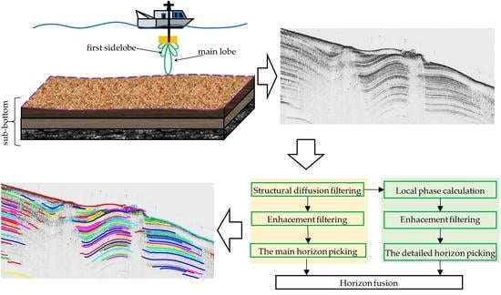
To overcome these limitations and to develop an effective automatic horizon picking method, we propose an integrated horizon picking method for obtaining the main and detailed horizons simultaneously. First, diffusion filtering is applied to the SBP image, and the smoothed reflectors can be obtained. The enhancement filtering is then introduced, and the main horizons are obtained. Next, the local phase image is obtained through monogenetic signal analysis, and the enhancement filtering is applied to the local phase image to suppress false reflector structures, and the detailed horizons are obtained after that. Combining the main horizons and the detailed horizons, the final horizons can be obtained.
2. Methods
This chapter begins with a brief introduction of the operating principle of SBP, and the factors affecting horizon picking are analyzed. The main part of the proposed method is then presented. The flowchart of the proposed method is shown in Figure 1.
2.1. SBP Working Principle and Influencing Factors for Horizon Picking
2.1.1. SBP Working Principle
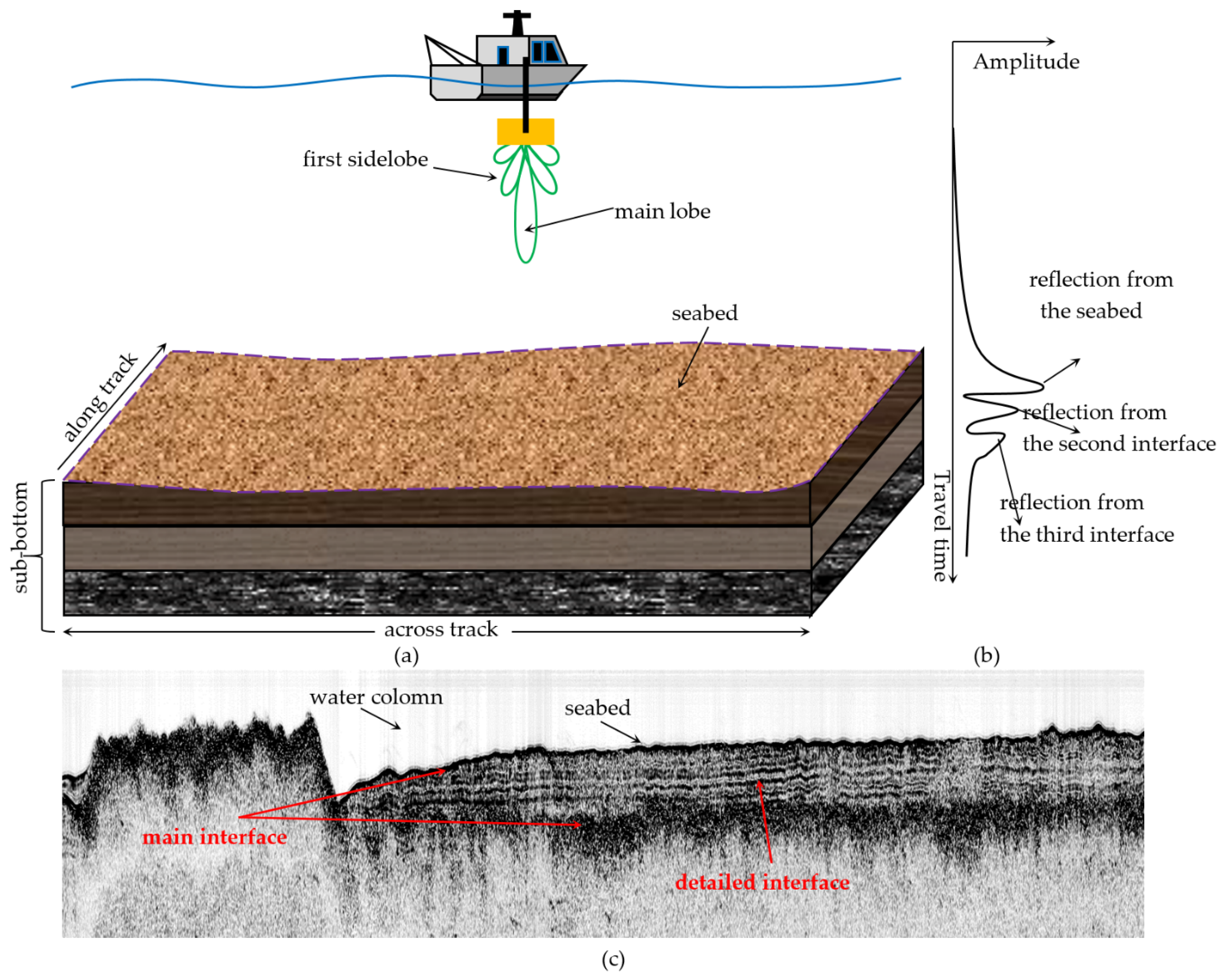
The working principles of SBP are shown in Figure 2a. The SBP sonar transmits an acoustic wave that is vertically aimed at the seafloor [1]. The acoustic wave is reflected back when it encounters an acoustic impendence difference interface, e.g., the seafloor or the interface between silt and sand. A large impendence difference can generate a large amplitude of the received acoustic amplitude, which can reflect the sediment property. Thus, the reflected acoustic waves carry information regarding the sediment properties, which are then received by the sonar.
The received acoustic signal, which is processed by Hilbert transformation, only provides the instantaneous amplitude (IA) data and these are usually used to build the SBP image [5]. Figure 2b shows the received acoustic IA data. Since the sub-bottom in Figure 2a consists of three different types of sediments, the received acoustic IA data have three peaks corresponding to the three reflectors, respectively, as shown in Figure 2b. These peaks show the depth information for the reflectors, and the horizon picking task is to obtain the locations of these peaks automatically.
A typical SBP image is shown in Figure 2c. The area without obvious reflections above the seabed is known as the water column (WC) area. The WC area reflects the water environment between the transducer and the seabed. In this paper, the reflector with a high amplitude and a relatively obvious thickness on the SBP image is named as the main reflector, and the corresponding picked horizon is named as the main horizon, as shown in Figure 2c. The reflector with a low amplitude and a thin thickness on the SBP image is named as the detailed reflector, and the corresponding picked horizon is named as the detailed horizon. Horizon picking is an important step of SBP data processing, which directly affects the analysis of data and their follow-up applications.
2.1.2. Factors Affecting Horizon Picking
1. The discontinuity of the peaks of the received echo sequence: The peak in a vertical local neighborhood can be recognized as a horizon point when satisfying some criteria. Theoretically, peaks representing the same reflector are continuous along the track. However, because of the attitude changes of the survey ship and complex sediments, these peaks may be discontinuous, bringing difficulties to post-processing and attribute analysis for the horizons [3].
2. Intensity imbalance: There are intensity imbalance phenomena in SBP images. Since the acoustic energy decreases when the travel time increases, the reflections from the deep sediment interface have low intensity compared to the reflections from the shallow sediment interface [5]. It is then difficult to pick all of the reflections using several intensity thresholds.
3. Scale parameter setting: Multi-scale horizon picking methods need require the setting of the scale parameter. A large-scale parameter setting can lose detailed horizons. A small-scale parameter can help pick detailed horizons. However, some reflections caused by noise will also be picked as horizons, which induce outliers in the final picked result [3,18].
2.2. Picking Method
2.2.1. Diffusion Filtering
Diffusion filtering has been widely used in local structure preserving and noise filtering. Seismic data processing research has used diffusion methods to smooth coherences. Since there are many similarities between SBP data processing and seismic data processing, diffusion filtering is also employed here to help obtain continuous reflectors.
First, the scatter matrix is introduced. u is the input image, and the scatter matrix reflecting the local structure of the image is then defined as [19,20]:
where , , are the first order partial derivatives of u along the x1 direction and the x2 direction. To avoid the influence of noise, u(x) is convolved with a Gaussian kernel kσ: uσ(x) = ( kσ∗u)(x). A new scatter matrix Jρ is then obtained as:
The scatter matrix is positively semidefinite and has orthonormal eigenvectors Vec1, Vec2, with Vec1 parallel to
where jlk (l = {1,2}, k = {1,2}) are the elements of the matrix Jρ(▽uσ). The vector Vec1 points out the orientation maximizing energy (namely, the gray-level) fluctuations, while Vec2 gives the preferred local smoothing direction. The eigenvalues corresponding to Vec1 and Vec2 are given by
The eigenvalues μ1 and μ2 indicate the local structural information. Isotropic structures exist when ; line-like structures exist when μ1 ≫ μ2 ≈ 0, and corners exist when μ1 ≥ μ2 ≫ 0. The nonlinear diffusion process is governed by a parabolic equation that can be viewed as [20]:
where N is the unit outward normal. Since the eigenvectors of D should reflect the local structure on the SBP image, one should choose the same orthonormal basis of eigenvectors as one gets from Jρ(▽uσ). The choice of the corresponding eigenvalues λ1 and λ2 of D depends on the desired goal. In this paper, we want to smooth preferably within each region and aim to preserve the edges. This may be achieved by the following choice of the eigenvalues of D(Jρ):
Through solving Equation (6), one can then obtain the image after diffusion filtering, and the final u after iteration solving is the filtered result.
2.2.2. Enhancement Filtering Algorithm
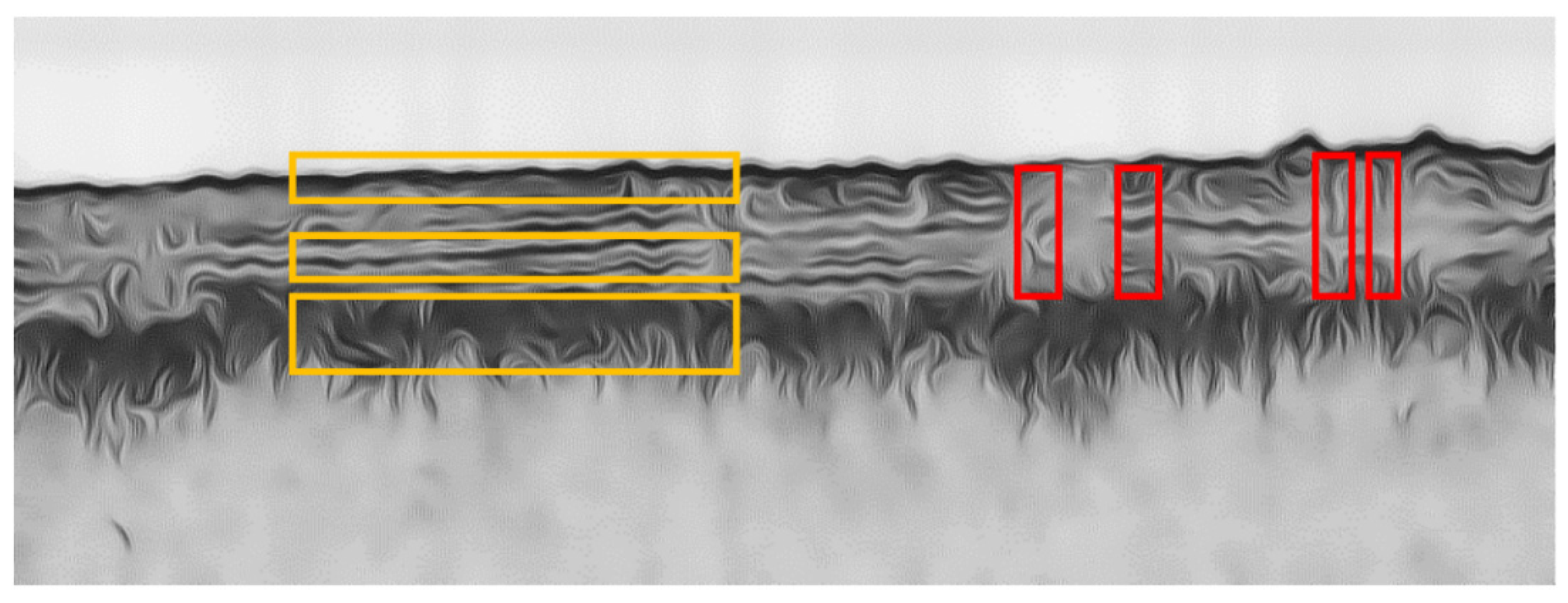
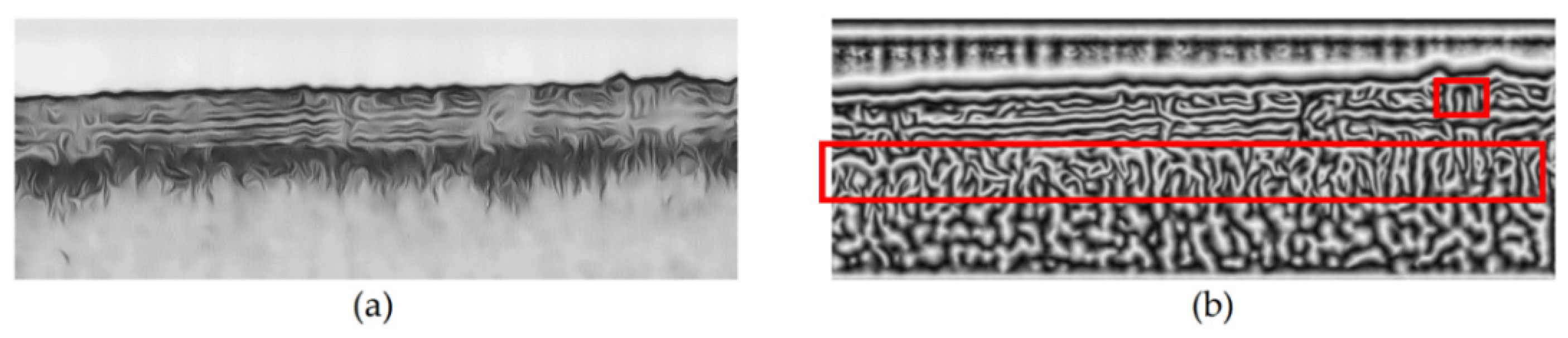
Enhancement filtering is applied to the image after diffusion filtering. As shown in Figure 3, the yellow rectangles mark several reflectors that extend along the horizontal direction. These reflectors can be recognized as line-like structures, and some filtering methods can be employed to enhance these structures and eliminate interference echoes [3,18]. Thus, an improved line-like structure enhancement filtering method is used to highlight reflectors and suppress interference.
At first, the Hessian matrix is introduced. The Hessian matrix corresponding to the pixel at x(x, y) is noted as H(x). H(x) = [Gxx(x)*I(x), Gxy*I(x); Gyx(x)*I(x), Gyy(x)*I(x)]. The original image is I(x). Gxx(x), etc., are the second order partial derivatives of G(x, σ0). G(x, σ0) is a Gaussian function, and σ0 is a scale parameter. Following the characteristics of Hessian matrix, the enhancement filtering can then be constructed as [3,26]
IM(σ0) is the SBP image after enhancement filtering when setting the scale parameter as σ0. RB and S as well as V have the same size as the original SBP image and are the descriptors for describing the local structure characteristics of every pixel in the original SBP image. RB characterizes the line-like structure, S characterizes the structure with high gray levels on the SBP image, and V is used to suppress the vertical structure. λ1, λ2 are the eigenvalues of matrix H(x) at every pixel in the original SBP image. β and c have suggested values [26]. a and m are set as 0.69 and 0.44 as suggested in [3].
Using RB, some blob-like structures can be suppressed. Using S, some reverberations can be eliminated. V is added to suppress some vertical structures. There are several intensity imbalance phenomena along the track which bring false vertical structures to the filtered result in the red rectangles in Figure 3. The addition of V can eliminate these false structures.
The parameter φ in Equation (9) is related to direction information, and it can be calculated through the method described as below. First, we assume that v1 and v2 are two eigenvectors of the Hessian matrix H(x) of a pixel (p, q) in the original SBP image. v2, corresponding to the smaller eigenvalue, represents the principal direction. Second, after setting eigenvector v2 = (Lp, Lq) (Lp and Lq corresponding to the x-coordinate and y-coordinate of v2 respectively), direction information φ is constructed as
The final multi-scale enhanced result is then obtained using:
In Equation (11), σmax corresponds to half of the thickness of the main reflector, and σmin corresponds to half the thickness of the detailed reflector.
2.2.3. Main Horizon Picking
Picking main horizons is employed based on the SBP image after diffusion filtering and the enhancement filtering. The threshold method is often adopted in horizon picking. In this method, we assume that the gray level of the pixels belonging to a reflector is higher than a given threshold [3]. For the main horizon picking, the following rule is adopted:
where Gp(m) is the gray level of the mth sampling point in a ping; μp and δp are the mean and standard deviation of the pixel gray levels in this ping; and h is the threshold, which is usually set to 2. If the gray level of a pixel satisfies Equation (12) and is a peak in a local vertical neighborhood, then the pixel is determined as a horizon point. After detecting all of the pings, the main horizon image is formed by setting the accepted horizon points to 255 and all others to 0.
2.2.4. Obtaining Local Phase Image
Through diffusion filtering, many reflectors have been smoothed. However, some reflectors are strictly not composed of edge or coherence structures, which have low intensity, even after diffusion filtering. Thus, the main horizon picking may ignore many detailed reflectors with low intensity. The local phase is introduced to solve this problem based on the image after diffusion filtering. The local phase in the field of monogenic signal analysis is employed to highlight local structures. The local phase image removes the influences of intensity variations and is usually used for detecting line-like structures [5,27,28,29].
The details for obtaining the local phase image are described as follows: For a 2-D signal f(x) (x = [x1, x2]T), the combination of a signal f(x) with its transform forms a 2-D generalization of the analytic signal, and the monogenic signal is obtained through [27,28]:
where and are quaternion units, and fM(x) is the monogenic signal corresponding to f(x). B is the band-pass filter (b is the spatial formation of B) with the transfer function and is used as follows:
where wl is the centre-wavelength expressed in pixel units, and wl is determined by the average scale parameter. h1 and h2 represent the spatial formation of the convolution kernel of the Riesz transform Hl(l{1,2}):
The local phase φ(x) is then obtained using:
Setting the enhanced image IM(σ) as a 2-D signal, namely f(x), through Equations (13)–(16), the local phase image ϕ(x) can then be obtained.
2.2.5. Phase Image Enhancement Filtering and the Detailed Horizon Picking
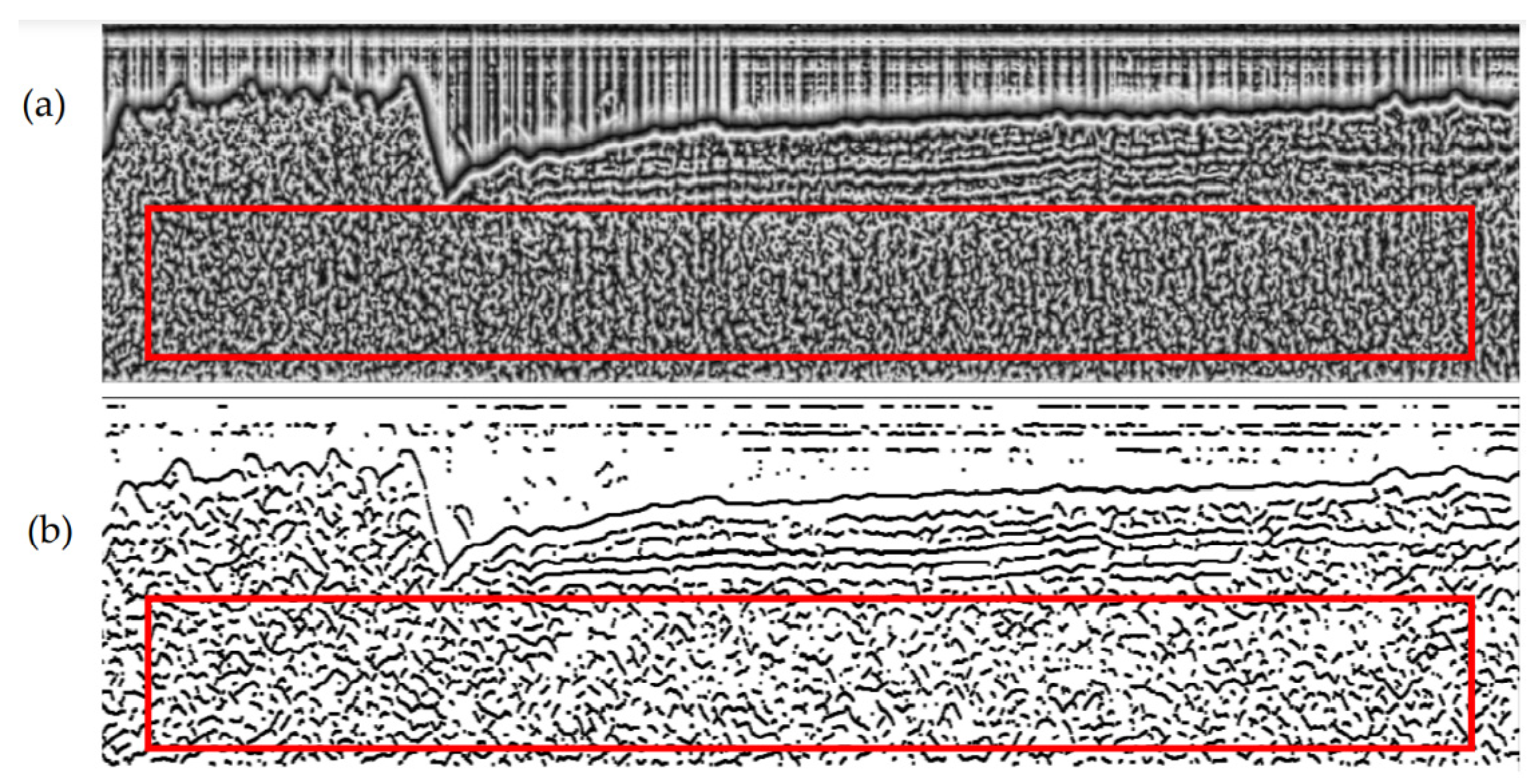
The SBP image after diffusion filtering and local phase calculation are shown in Figure 4a,b. There are intensity imbalance phenomena on the original SBP image distributed along the vertical direction, and these vertical imbalance structures will be specifically highlighted after diffusion filtering and local phase calculation. Thus, there are lots of false structures (as shown in Figure 4b marked with red rectangles) along the vertical direction. To eliminate these false structures and enhance the reflector structures, enhancement filtering can be applied to the phase image. The method described in Equation (12) is also applied to pick the detailed horizon points based on the local phase image after enhancement filtering.
Through the above process steps, all of the detailed horizon points can be obtained. These horizon points that are close to each other in 3 × 3 neighborhoods will be recognized as horizon points belonging to the same horizon segment (for example, the green points and blue points in Figure 5 can constitute two horizon segments). Every horizon point belonging to the same horizon segment will be assigned a label. A new image (called detailed horizon image) is formed by setting the detailed horizon points (p, q) as 255 and the others as 0.
2.2.6. Horizon Fusion
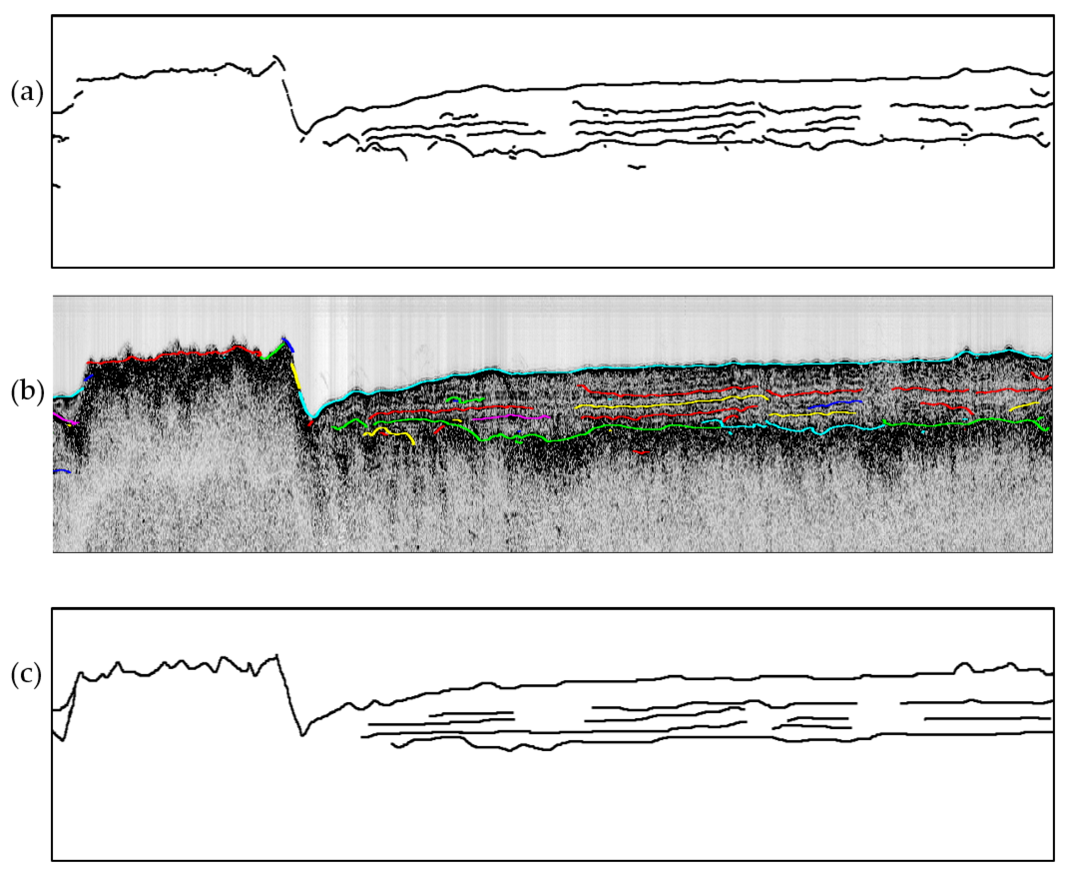
Compared to the main horizons, detailed horizons have advantages in terms of continuity and detailed degree, while the main horizon result has fewer outliers. We then assume that the blue, the green points, and the black points in Figure 5 are the picked detailed horizons, and the red points in Figure 5 are the main horizons. The black points are outliers that should be removed at the end. We then fuse the main horizons and the detailed horizons in this section.
Centered at every main horizon point, neighborhoods along the vertical direction can be defined. As shown in Figure 5, the yellow shadowed areas show the neighborhoods defined by the red main horizon points. Detailed horizon points that are located in the yellow shadowed areas can then be found by traversing the yellow areas. Since every detailed horizon point is assigned a label, the labels of the detected detailed horizon point can then be obtained after traversing the yellow shadowed areas in Figure 5. After that, all of the detailed horizon points corresponding to the obtained labels can be extracted, which means that all of the green and blue horizon points in Figure 5 can be obtained. If the length of the extracted detailed horizon segment is larger than the length of the corresponding main horizon segment, the extracted detailed horizon segment will remain, while the corresponding main horizons will be removed, otherwise, the extracted horizon segment will be removed as outliers while the main horizons remain. All of the detailed horizon points with the constraints of the main horizon points can be obtained. Outliers such as the black points in Figure 5 will be removed.
3. Experiment and Results
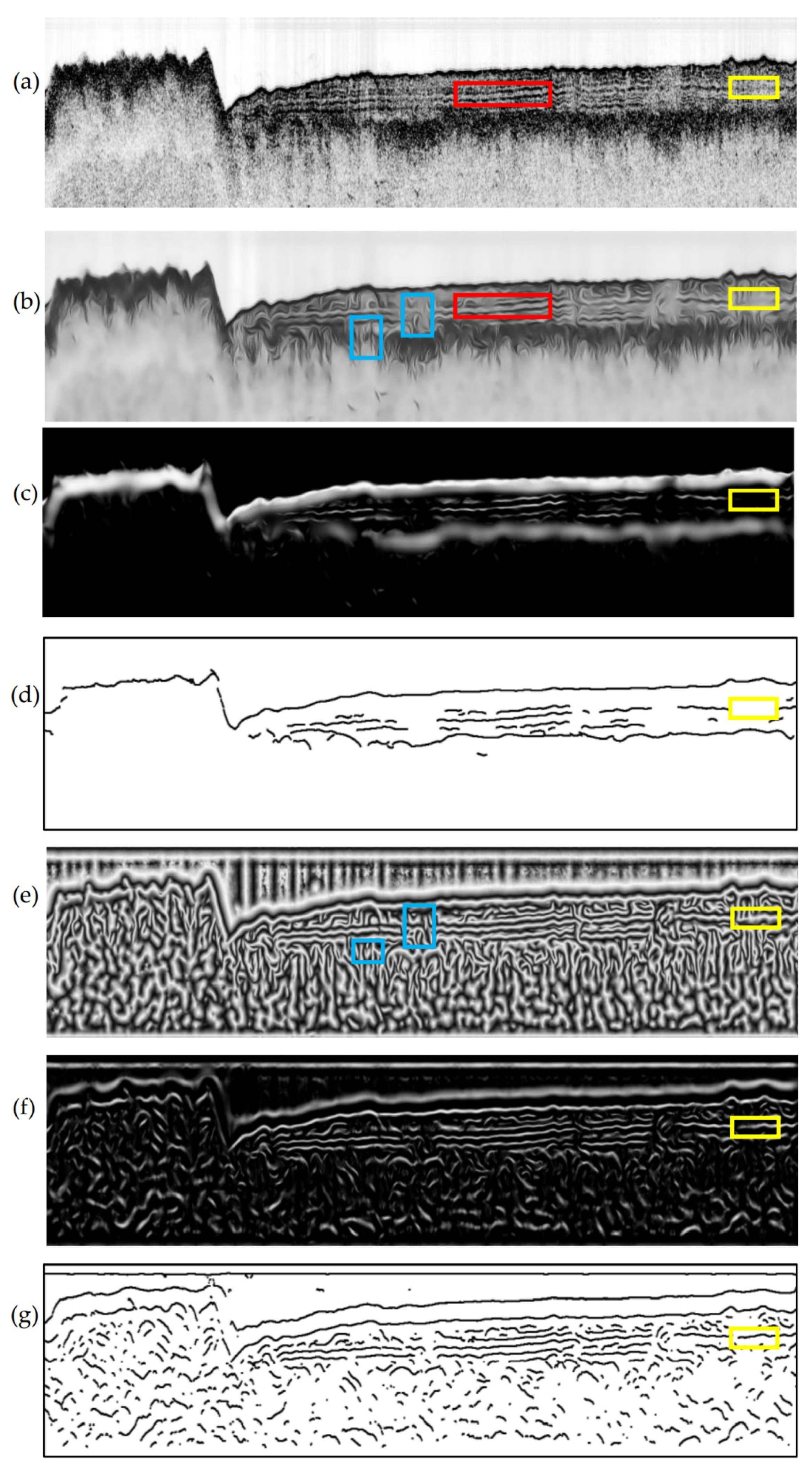
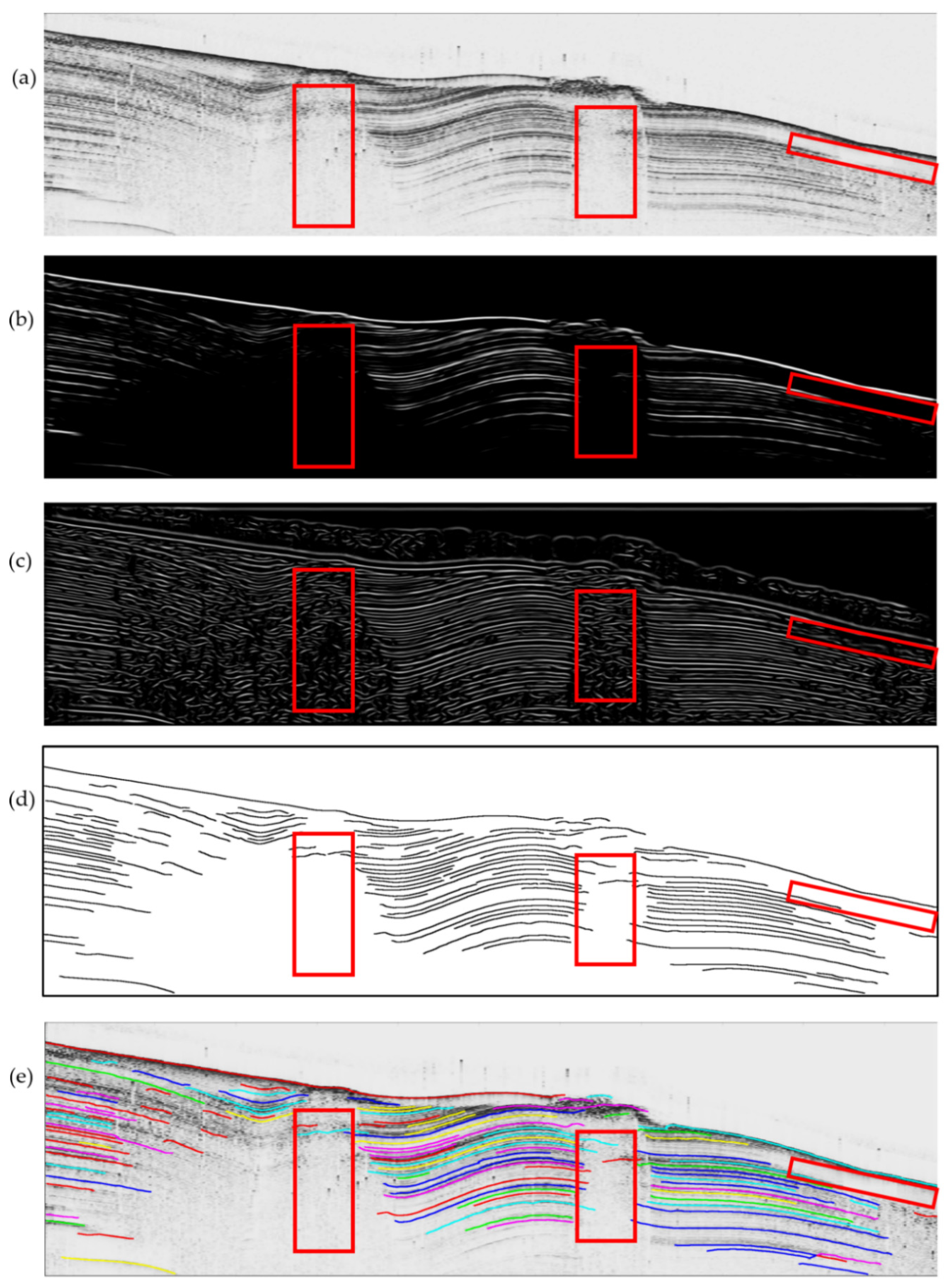
In order to verify the effectiveness of the proposed method, the raw data collected by SBP sonars were selected for the experiments. Figure 6a shows an SBP image surveyed in ShenZhen in 2016. During the survey, the transducer was mounted on a fishing vessel in an outboard mode. The water depth in the surveyed area varies from 5 m~15 m. The sediment there mainly consists of silt and sand. A total of two main reflectors could be found, and there were many tiny parallel reflections inside the first main layer.
First, diffusion filtering was applied to Figure 6a. The filtered result is shown in Figure 6b. The tiny reflections in the red rectangle were well-smoothed, and the continuity of these reflections became more obvious than before. Diffusion filtering simulates the process of energy diffusion. The energy (namely the gray-level) diffusing along the vertical direction is caused by the intensity imbalance on SBP image along the vertical direction. The process of vertical diffusion can generate false vertical structures in the blue rectangle areas in Figure 6b. Figure 6c shows the results of applying the enhancement filtering method to Figure 6b. Note that the false structures in Figure 6b were suppressed because the vertical suppress term designed in Equation (8) can suppress vertical structures. Based on the result in Figure 6c, the threshold picking method was then employed, and the picked horizons were shown in Figure 6d. It can be seen that the main horizons have been obtained, and part of the detailed horizons also have been picked.
Comparing Figure 6a to Figure 6b, the reflectors in the area marked by a yellow rectangle in Figure 6a disappeared in Figure 6b, and these reflectors were also not enhanced after enhancement filtering in Figure 6c. In fact, structures in the yellow rectangle are not very similar to the edge-like structures even though the diffusion filtering method is good at filtering the edge-like structures. Thus, the local phase was employed, and the local phase of Figure 6b is shown in Figure 6e. All of the reflections have been highlighted, even the structures in the area marked by a yellow rectangle. Still, false structures were found in Figure 6e (marked with blue rectangles). To suppress these false structures in Figure 6e, enhancement filtering was also used. Thanks to the designed vertical suppress term, many vertical false structures disappeared in Figure 6f. The threshold picking was then applied to Figure 6f, and the horizons were obtained, as shown in Figure 6g. The detailed horizons were kept well, although some outliers still remained. To remove these outliers and obtain integrated horizons, we fused the main horizons with the detailed horizons. The final horizons are shown in Figure 7a. Figure 7b shows the superposition of the original SBP image and the horizon image. The main and detailed horizons were all well picked and the outliers have been removed. Comparing the result in Figure 7a with that in Figure 6d, the result in Figure 7a shows more detailed horizons. Comparing the result in Figure 7a with that in Figure 6g, the main horizons have been well-kept, and the outliers were well-removed.
To quantitatively evaluate the picked horizons in Figure 7a, the ground truth should be obtained first. Through visual interpretation, horizons picked manually were used as ground truth and are shown in Figure 7c. Classic detection accuracy metrics, such as precision, recall, F-measure, and accuracy [3], were used to verify the picked result. Taking the ground truth as the reference, the picked horizons in Figure 7a were evaluated on the basis that a horizon point is deemed to be correct if the vertical distance between it and its reference was smaller than seven pixels. The statistical results are shown in Table 1. An F-measure value of 87%, and an accuracy of 99% were achieved.
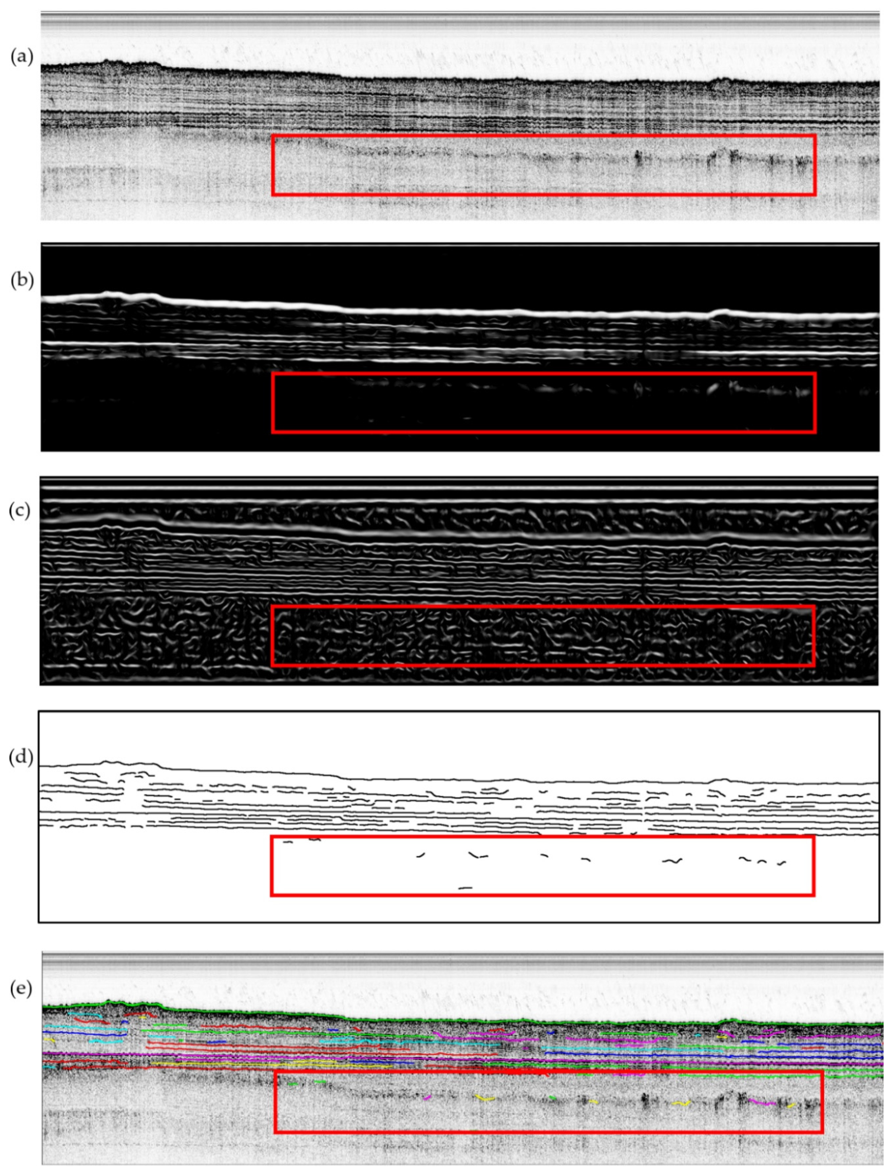
We also applied the proposed horizon picking algorithm to a case where a wealth of detailed horizons exists. Figure 8a shows an SBP image with plenty of detailed horizons. Here, we only display part of the images for simplicity. The images after diffusion filtering and local phase calculation were not displayed. Figure 8b shows the filtered image used for the main horizon picking, and several reflectors with relatively high intensity have been enhanced. However, some reflectors with thin thickness and low intensity were not highlighted, and some are nearly invisible in Figure 8b. Figure 8c shows the filtered image based on the local phase image. Since the local phase image highlighted all of the reflectors, the detailed horizons can be well-obtained. Fusing the main horizons and the detailed horizons, the final horizons are shown in Figure 8d. Figure 8e shows the superposition of the original SBP image and the horizon image, and the picked horizons have good consistency with the reflectors on the original SBP image.
There is a remarkable phenomenon in this experiment, which is that the reflectors caused by scattered echoes cannot be well-picked. As shown in the red rectangle in Figure 8a, these reflections representing multiples are mainly composed of scatters and are not very similar to the line-like structures that can be well enhanced through the enhancement filtering method. Nevertheless, for the main and detailed reflectors we are concerned about, the proposed method achieved good results.
To further verify the performance of the proposed method during deep-sea mineral resources survey, an SBP image (Figure 9a) obtained using the Parasound P70 SBP sonar in the South China Sea in 2016 with the water depths ranging from 400 m to 2400 m was used to pick the main and detailed horizons. During the survey, the transducer was mounted on an oceanic research vessel in towed mode. Figure 9b shows the filtered image used for the main horizon picking, and Figure 9c shows the filtered image based on a local phase image. Figure 9d shows the picked results, and Figure 9e shows the superposition of the picked horizons with the original SBP image. There are three acoustic blank areas marked with red rectangles, and these acoustic blanks indicate the traces of gas migration. Acoustic blank areas can be well-described by the distribution and changes of the main and detailed horizons and can help interpreters to discover and analyze marine mineral sources.
4. Discussion
4.1. The Contributions of These Processing Steps
There are three main processing steps in the proposed method, namely diffusion filtering, enhancement filtering, and local phase calculation. We conducted several experiments to analyze the contributions of these steps.
The diffusion filtering: Both the main horizon picking and the detailed horizon picking need diffusion filtering to provide smooth reflectors on the SBP image. Section 4.2 will discuss the contribution of diffusion filtering to the picking of the main horizon. Here, we calculate the local phase without diffusion filtering and picked the detailed horizons to analyze the contribution of diffusion filtering on detailed horizon picking. The calculated local phase image without diffusion filtering is shown in Figure 10a, and the corresponding horizons are shown in Figure 10b. Compared to the local phase image in Figure 6e, the reflectors in Figure 10a are not obvious enough. The picked horizons in Figure 10b include many outliers (marked with red rectangles), which may create difficulties for horizon fusing. It can be concluded that the diffusion filtering method is very helpful for continuous horizon picking and for the elimination of outliers.
The local phase calculation: Some reflectors with low intensity can be enhanced in local phase images. Comparing the main horizons in Figure 6d with the detailed horizons in Figure 6g, more continuous horizons were obtained from the local phase images.
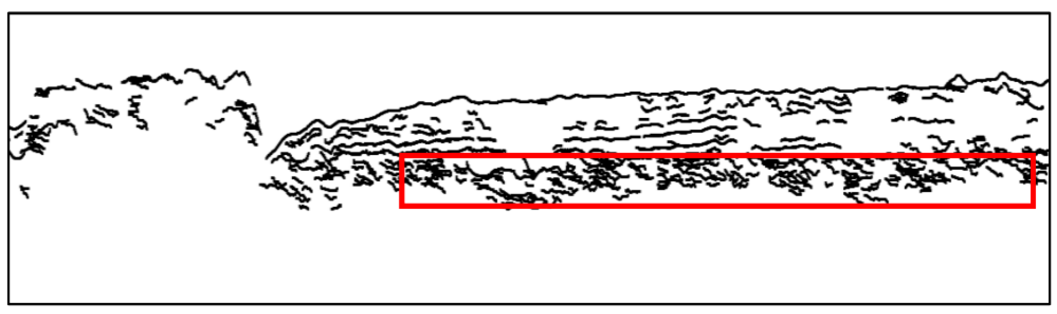
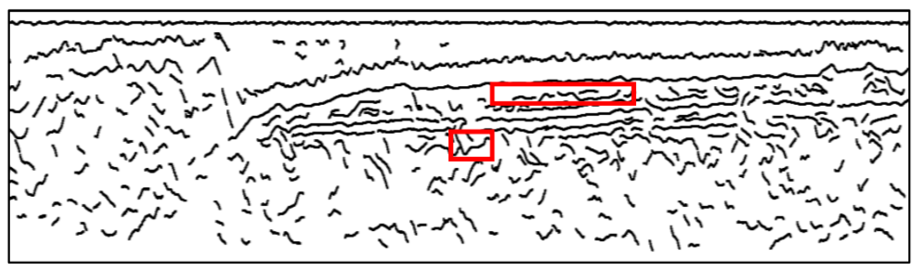
The enhancement filtering: The effectiveness of the enhancement filtering method on the main horizon picking has been well described in [3]. Here, the detailed horizons that were picked without enhancement filtering were analyzed. Figure 11 and Figure 12 show the horizons picked from the image after diffusion filtering and from the local phase image without enhancement filtering. Many outliers caused by vertical false structures and discrete sediment interfaces are shown in the area marked with red rectangles in Figure 11 and Figure 12. It can be concluded that the enhancement filtering method enhances line-like structures well and weakens the effect of noise, and the vertical suppression term maintains the actual horizons and removes false vertical horizons.
4.2. Comparsion with the FrangiV Method
The FrangiV method is a horizon picking method based on enhancement filtering and threshold picking algorithms [3]. The FrangiV method modified the traditional multi-scale filtering method proposed by Frangi by adding a vertical suppression term that can suppress false vertical structures on SBP images. We applied the FrangiV method to Figure 6a and picked horizons. During filtering, different sets of scale parameters were used, and different filtered results were obtained, as shown in Figure 13a,c. The scale parameters used in Figure 13a were smaller than those used in Figure 13c. The picked horizons in Figure 13b show more detailed horizons than the one shown in Figure 13d. The performances of both Figure 13b,d are poorer than Figure 7a, especially in the areas marked with red rectangles. Table 2 and Table 3 show the results comparing Figure 13c,d with the ground truth in Figure 7c. The proposed method achieved a higher F-measure value compared to the FrangiV method from Table 1, Table 2 and Table 3. Comparing Figure 13a with Figure 6c, more detailed horizons were displayed in Figure 6c, which indicates the effectiveness of diffusion filtering in the proposed method.
Theoretically speaking, the diffusion filtering used in this paper can preserve all edges and can maintain tiny reflectors. The local phase calculation used in this paper avoids missing horizons caused by the single threshold picking algorithm used in the FrangiV method. Thus, detailed horizons can be well picked. The integrated method proposed here based on diffusion filtering, enhancement filtering, and local phase calculation can obtain the main and detailed horizons on SBP image and can achieve good performance.
4.3. Limitations and Future Works
Reflectors caused by scattered echoes cannot be picked well using the proposed method since these reflections are not very similar to the line-like structures that can be enhanced using an enhancement filtering method. These scattered echoes may be caused by multiples or the bedrock. Although multiples are neglectable in most cases, they can be used to calculate reflection coefficients [30]. The bedrock is also very important for geographical interpretation. Thus, more attention should be paid to picking horizons from scattered echoes in the future.
Nowadays, deep learning has been developed to work out tough tasks in the field of sonar data processing and sonar target recognition and has achieved better performances than traditional methods [31,32,33]. Our future work, then, is to develop a method combining the framework of deep learning and local phase images to obtain the main and detailed horizons.
5. Conclusions
This paper proposes an integrated method based on diffusion filtering, enhancement filtering, and local phase calculation to obtain the main and detailed horizons on a SBP image and is verified by data measured in different cases. Experiments show that the method is able to provide good results. The diffusion filtering method smooths the line-like structures of the reflectors and eliminates noise at the same time. The local phase image highlights all of the reflections and is quite important for obtaining the detailed horizons. Enhancement filtering enhances line-like structures well and weakens the effect of noise. The suppression of vertical structures in enhancement filtering can maintain the actual horizons and suppress false vertical structures in images after diffusion filtering and local phase calculation, which allows accurate horizon picking. In future work, we will further extend the method to pick horizons representing scattered echoes and combine this method with a deep learning framework to achieve better results and to realize real-time SBP horizon picking.
Author Contributions
Conceptualization, S.L., J.Z. and H.Z.; funding acquisition, J.Z.; investigation, S.L. and J.Z.; methodology, S.L. and J.Z.; software, S.L.; supervision, J.Z. and H.Z.; visualization, S.L. and S.Q.; writing—original draft, S.L.; writing—review and editing, J.Z., H.Z. and S.Q. All authors have read and agreed to the published version of the manuscript.
Funding
This research was funded by the National Natural Science Foundation of China under Grant 41576107 and Grant 41376109.
Data Availability Statement
Access to the data will be considered upon request by the authors.
Acknowledgments
We would like to thank the editor and the anonymous reviewers for their valuable comments and suggestions that have greatly improved the quality of this paper.
Conflicts of Interest
The authors declare no conflict of interest.
References
- Lurton, X. An Introduction to Underwater Acoustic: Principles and Applications, 2nd ed.; Springer: Chichester, UK, 2010; pp. 372–379. [Google Scholar]
- Li, S.; Zhao, J.; Zhang, H.; Bi, Z.; Qu, S. A Non-Local Low-Rank Algorithm for Sub-Bottom Profile Sonar Image Denoising. Remote Sens. 2020, 12, 2336. [Google Scholar] [CrossRef]
- Li, S.; Zhao, J.; Zhang, H.; Bi, Z.; Qu, S. A Novel Horizon Picking Method on Sub-Bottom Profiler Sonar Images. Remote Sens. 2020, 12, 3322. [Google Scholar] [CrossRef]
- Zhao, J.; Li, S.; Zhang, H.; Feng, J. Comprehensive Sediment Horizon Picking from Subbottom Profile Data. IEEE J. Ocean. Eng. 2019, 44, 524–534. [Google Scholar] [CrossRef]
- Zhao, J.H.; Li, S.B.; Zhao, X.; Feng, J. A Comprehensive Horizon-picking Method on Sub-bottom Profiles by Combining Envelope, Phase Attributes, and Texture Analysis. Earth Space Sci. 2020, 7, 1–20. [Google Scholar] [CrossRef] [Green Version]
- Maroni, C.S.; Quinquis, A.; Vinson, S. Horizon Picking on Sub-bottom Profiles Using Multiresolution Analysis. Digit. Signal Prog. 2001, 11, 269–287. [Google Scholar] [CrossRef]
- Bondár, I. Seismic Horizon Detection Using Image Processing Algorithms. Geophys. Prospect. 1992, 40, 785–800. [Google Scholar] [CrossRef]
- Idczak, J.; Brodecka-Goluch, A.; Łukawska-Matuszewska, K.; Graca, B.; Gorska, N.; Klusek, Z.; Pezacki, P.D.; Bolałek, J. A Geophysical, Geochemical and Microbiological Study of a Newly Discovered Pockmark with Active Gas Seepage and Submarine Groundwater Discharge (MET1-BH, central Gulf of Gdańsk, southern Baltic Sea). Sci. Total Environ. 2020, 742, 140306. [Google Scholar] [CrossRef] [PubMed]
- Hoffmann, J.J.L.; von Deimling, J.S.; Schröder, J.F.; Schmidt, M.; Held, P.; Crutchley, G.J.; Scholten, J.; Gorman, A.R. Complex Eyed Pockmarks and Submarine Groundwater Discharge Revealed by Acoustic Data and Sediment Cores in Eckernförde Bay, SW Baltic Sea. Geochem. Geophys. Geosyst. 2020, 21, 1–18. [Google Scholar] [CrossRef]
- Garcia-Gil, S.; Vilas, F.; Garcia-Garcia, F. Shallow Gas Features in Incised-valley Fills (Rıa de Vigo, NW Spain): A case study. Cont. Shelf Res. 2002, 22, 2303–2315. [Google Scholar] [CrossRef]
- Kato, Y.; Fujinaga, K.; Nakamura, K.; Takaya, K.; Kitamura, K.; Ohta, J.; Toda, R.; Nakashima, T.; Iwamori, H. Deep-sea Mud in the Pacific-ocean as a Potential Resource for Rare-earth Elements. Nat. Geosci. 2011, 4, 535–539. [Google Scholar] [CrossRef]
- Song, W.; Wu, X.; Yang, T.; Huang, W.; Wang, Q. Application of Japanese SBP Data on Deep-sea REY Survey and Implications. China Min. Mag. 2019, 28, 173–180. [Google Scholar] [CrossRef]
- Fakiris, E.; Blondel, P.; Papatheodorou, G.; Christodoulou, D.; Dimas, X.; Georgiou, N.; Kordella, S.; Dimitriadis, C.; Rzhanov, Y.; Geraga, M.; et al. Multi-frequency, Multi-sonar Mapping of Shallow Habitats Efficacy and Management Implications in the National Marine Park of Zakynthos, Greece. Remote Sens. 2019, 11, 461. [Google Scholar] [CrossRef] [Green Version]
- Dossi, M.; Forte, E.; Pipan, M. Automated Reflection Picking and Polarity Assessment through Attribute Analysis: Theory and Application to Synthetic and Real Ground-penetrating Radar Data. Geophysics 2015, 80, 23–35. [Google Scholar] [CrossRef]
- Forte, E.; Dossi, M.; Pipan, M.; Ben, A.D. Automated Phase Attribute-based Picking Applied to Reflection Seismics. Geophysics 2016, 81, 55–64. [Google Scholar] [CrossRef]
- Kim, Y.J.; Koo, N.H.; Cheong, S.; Kim, J.K.; Chun, J.H.; Shin, S.R.; Riedel, H.; Lee, Y.H. A Case Study on Pseudo 3-D Chirp Sub-bottom Profiler (SBP) Survey for the Detection of a Fault Trace in Shallow Sedimentary Layers at Gas Hydrate Site in the Ulleung Basin, East Sea. J. Appl. Geophys. 2016, 133, 98–115. [Google Scholar] [CrossRef]
- Baradello, L. An Improved Processing Sequence for Uncorrelated Chirp Sonar Data. Mar. Geophys. Res. 2014, 35, 337–344. [Google Scholar] [CrossRef]
- Wang, W.; Ren, Q.; Li, J.; Ma, L. Hybrid Method to Extract Sediment Layered Structure from Sub-bottom Profile. In Proceedings of the 2017 IEEE International Conference on Signal Processing, Communications and Computing (ICSPCC 2017), Xiamen, China, 22–25 October 2017; pp. 1–4. [Google Scholar] [CrossRef]
- Perona, P.; Malik, J. Scale-space and Edge Detection Using Anisotropic Diffusion. IEEE Trans. Pattern Anal. 1990, 12, 629–639. [Google Scholar] [CrossRef] [Green Version]
- Weicker, J. Coherence Enhancing Diffusion Filtering. Int. J. Comp. 1999, 31, 111–127. [Google Scholar] [CrossRef]
- Fehmers, G.; Hocker, C. Fast Structural Interpretation with Structure-oriented filtering. Geophysics 2003, 68, 1286–1293. [Google Scholar] [CrossRef]
- Lavialle, O.; Pop, S.; Germain, C.; Donias, M.; Guillon, S.; Keskes, N.; Berthoumieu, Y. Seismic Fault Preserving Diffusion. J. Appl. Geophys. 2007, 61, 132–141. [Google Scholar] [CrossRef] [Green Version]
- Chopra, S.; Marfurt, K. Emerging and Future Trends in Seismic Attributes. Leading Edge 2008, 27, 298–318. [Google Scholar] [CrossRef]
- Wu, X.; Yan, S.; Qi, J.; Zeng, H. Deep Learning for Characterizing Paleokarst Collapse Features in 3-D Seismic Images. J. Geophys. Res. Sol. Earth 2020, 125, 1–23. [Google Scholar] [CrossRef]
- Shi, Y.; Wu, X.; Fomel, S. Interactively Tracking Seismic Geobodies with a Deep-learning Flood-filling Network. Geophysics 2021, 86, A1–A5. [Google Scholar] [CrossRef]
- Frangi, A.F.; Niessen, W.J.; Vincken, K.L.; Viergever, M.A. Multiscale Vessel Enhancement Filtering. In Proceedings of the International Conference on Medical Image Computing and Computer-Assisted Intervention (MICCAI1998), Boston, MA, USA, 11–13 October 1998; pp. 130–137. [Google Scholar] [CrossRef] [Green Version]
- Felsberg, M.; Sommer, G. The Monogenic Signal. IEEE Trans. Signal Process. 2002, 49, 3136–3144. [Google Scholar] [CrossRef] [Green Version]
- Picard, L.; Baussard, A.; Quidu, I.; Chenadec, G. Seafloor Description in Sonar Images Using the Monogenic Signal and the Intrinsic Dimensionality. IEEE Trans. Geosci. Remote. 2018, 56, 5572–5587. [Google Scholar] [CrossRef]
- Hidalgo-Gato, M.C.; Barbosa, V.C.F. The Monogenic Signal of Potential-field Data: A Python Implementation. Geophysics 2017, 82, 9–14. [Google Scholar] [CrossRef]
- Mohamed, S. Seabed Classification Using Sub- bottom Profiler. Master’s Thesis, Delft University of Technology, Delft, The Netherlands, 2011. [Google Scholar]
- Zhu, P.P.; Isaacs, J.; Fu, B.; Ferrari, S. Deep Learning Feature Extraction for Target Recognition and Classification in Underwater Sonar Images. In Proceedings of the 2017 IEEE 56th Annual Conference on Decision and Control (CDC), Melbourne, Australia, 12–15 December 2017. [Google Scholar] [CrossRef]
- Wang, Q.; Wu, M.H.; Yu, F.; Feng, C.; Li, K.G.; Zhu, Y.M.; Rigall, E.; He, B. RT-Seg: A Real-Time Semantic Segmentation Network for Side-Scan Sonar Images. Sensors 2019, 19, 1985. [Google Scholar] [CrossRef] [PubMed] [Green Version]
- Zheng, G.; Zhang, H.; Li, Y.; Zhao, J. A Universal Automatic Bottom Tracking Method of Side Scan Sonar Data Based on Semantic Segmentation. Remote Sens. 2021, 13, 1945. [Google Scholar] [CrossRef]
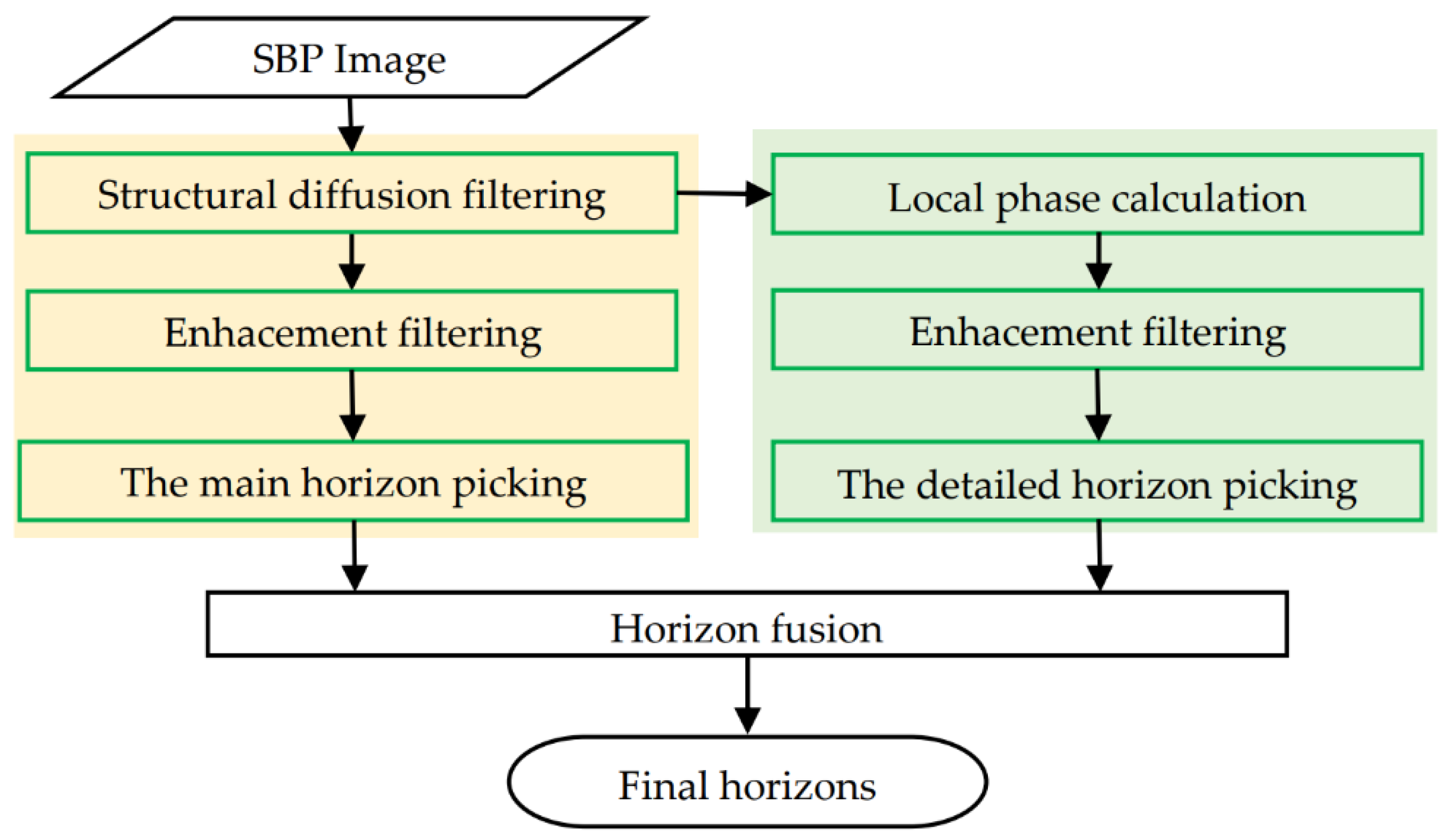
Figure 1.
Flowchart of the horizon picking method.

Figure 2.
Working principle of SBP. (a) shows the imaging principle of SBP. (b) shows the received acoustic IA data. (c) shows a typical SBP image.
Figure 2.
Working principle of SBP. (a) shows the imaging principle of SBP. (b) shows the received acoustic IA data. (c) shows a typical SBP image.

Figure 3.
SBP image characteristics after diffusion filtering. Yellow rectangles mark the line-like structures of reflectors. Red rectangles highlight the false vertical structures caused by intensity imbalance phenomena.
Figure 3.
SBP image characteristics after diffusion filtering. Yellow rectangles mark the line-like structures of reflectors. Red rectangles highlight the false vertical structures caused by intensity imbalance phenomena.

Figure 4.
Characteristics of processed SBP images. (a) shows the diffusion filtered SBP image. (b) shows the local phase image of (a).
Figure 4.
Characteristics of processed SBP images. (a) shows the diffusion filtered SBP image. (b) shows the local phase image of (a).

Figure 5.
Working principle of horizons fusion. The black, green, and blue points represent the detailed horizon points. Red points denote the main horizon points. Yellow rectangle shallowed areas show the vertical neighborhood of the red points.
Figure 5.
Working principle of horizons fusion. The black, green, and blue points represent the detailed horizon points. Red points denote the main horizon points. Yellow rectangle shallowed areas show the vertical neighborhood of the red points.

Figure 6.
Processed results of SBP image. (a) shows the original SBP image. (b) shows the SBP image after diffusion filtering. (c) shows the image after enhancement filtering based on (b). (d) shows the main horizons. (e) shows the local phase image based on (b). (f) shows the image after enhancement filtering based on (e). (g) shows the detailed horizons.

Figure 7.
Result of horizon picking. (a) shows the final horizons after horizon fusion. (b) shows the superposition of picked horizons with the original SBP image. Horizon points belonging to the same horizon segment are assigned the same color. (c) shows the ground truth obtained through manual picking.

Figure 8.
Processed results of SBP image. (a) shows the original SBP image. (b) the SBP image after enhancement filtering based on diffusion filtering result. (c) shows the SBP image after enhancement filtering based on local phase. (d) shows the final horizons. (e) shows the superposition of picked horizons with the original SBP image. Horizon points belonging to the same horizon segment are assigned the same color.

Figure 9.
Processed results of SBP image. (a) shows the original SBP image. (b) the SBP image after enhancement filtering based on diffusion filtering result. (c) shows the SBP image after enhancement filtering based on local phase image. (d) shows the final horizons. (e) shows the superposition of picked horizons with the original SBP image. Horizon points belonging to the same horizon segment are assigned the same color.

Figure 10.
Local phase and the detailed horizons without diffusion filtering. (a) shows the local phase image without diffusion filtering. (b) shows the detailed horizons picked from (a). Red rectangles show the outliers.
Figure 10.
Local phase and the detailed horizons without diffusion filtering. (a) shows the local phase image without diffusion filtering. (b) shows the detailed horizons picked from (a). Red rectangles show the outliers.

Figure 11.
The main horizons obtained without enhancement filtering. Red rectangle shows the discrete and wrong horizons.
Figure 11.
The main horizons obtained without enhancement filtering. Red rectangle shows the discrete and wrong horizons.

Figure 12.
The detailed horizons obtained without enhancement filtering. Red rectangles show the discrete and wrong horizons.
Figure 12.
The detailed horizons obtained without enhancement filtering. Red rectangles show the discrete and wrong horizons.

Figure 13.
Results using the FrangiV method. (a) shows the filtered result using the FrangiV method with small scale parameter settings. (b) shows horizons picked from (a). (c) shows the filtered result using the FrangiV method with large scale parameter settings. (d) shows horizons picked from (c).


Table 1.
Analysis of the picked horizons in Figure 7a.
Table 1.
Analysis of the picked horizons in Figure 7a.
| Precision | Recall | F-measure | Accuracy |
|---|---|---|---|
| 0.88 | 0.87 | 0.87 | 0.99 |
Table 2.
Analysis of the picked horizons in Figure 13b.
Table 2.
Analysis of the picked horizons in Figure 13b.
| Precision | Recall | F-measure | Accuracy |
|---|---|---|---|
| 0.89 | 0.82 | 0.85 | 0.99 |
Table 3.
Analysis of the picked horizons in Figure 13d.
Table 3.
Analysis of the picked horizons in Figure 13d.
| Precision | Recall | F-measure | Accuracy |
|---|---|---|---|
| 0.94 | 0.58 | 0.71 | 0.99 |
Publisher’s Note: MDPI stays neutral with regard to jurisdictional claims in published maps and institutional affiliations. |
© 2021 by the authors. Licensee MDPI, Basel, Switzerland. This article is an open access article distributed under the terms and conditions of the Creative Commons Attribution (CC BY) license (https://creativecommons.org/licenses/by/4.0/).
Share and Cite
MDPI and ACS Style
Li, S.; Zhao, J.; Zhang, H.; Qu, S. An Integrated Horizon Picking Method for Obtaining the Main and Detailed Reflectors on Sub-Bottom Profiler Sonar Image. Remote Sens. 2021, 13, 2959. https://doi.org/10.3390/rs13152959
AMA Style
Li S, Zhao J, Zhang H, Qu S. An Integrated Horizon Picking Method for Obtaining the Main and Detailed Reflectors on Sub-Bottom Profiler Sonar Image. Remote Sensing. 2021; 13(15):2959. https://doi.org/10.3390/rs13152959
Chicago/Turabian StyleLi, Shaobo, Jianhu Zhao, Hongmei Zhang, and Siheng Qu. 2021. "An Integrated Horizon Picking Method for Obtaining the Main and Detailed Reflectors on Sub-Bottom Profiler Sonar Image" Remote Sensing 13, no. 15: 2959. https://doi.org/10.3390/rs13152959
Note that from the first issue of 2016, this journal uses article numbers instead of page numbers. See further details here.