Article

Remote Sensing Estimation of Bamboo Forest Aboveground Biomass Based on Geographically Weighted Regression

1
State Key Laboratory of Subtropical Silviculture, Zhejiang A & F University, Hangzhou 311300, China
2
Key Laboratory of Carbon Cycling in Forest Ecosystems and Carbon Sequestration of Zhejiang Province, Zhejiang A & F University, Hangzhou 311300, China
3
School of Environmental and Resources Science, Zhejiang A & F University, Hangzhou 311300, China
*
Author to whom correspondence should be addressed.
Remote Sens. 2021, 13(15), 2962; https://doi.org/10.3390/rs13152962
Submission received: 30 June 2021 / Revised: 18 July 2021 / Accepted: 19 July 2021 / Published: 28 July 2021

Abstract

:
Bamboo forests are widespread in subtropical areas and are well known for their rapid growth and great carbon sequestration ability. To recognize the potential roles and functions of bamboo forests in regional ecosystems, forest aboveground biomass (AGB)—which is closely related to forest productivity, the forest carbon cycle, and, in particular, carbon sinks in forest ecosystems—is calculated and applied as an indicator. Among the existing studies considering AGB estimation, linear or nonlinear regression models are the most frequently used; however, these methods do not take the influence of spatial heterogeneity into consideration. A geographically weighted regression (GWR) model, as a spatial local model, can solve this problem to a certain extent. Based on Landsat 8 OLI images, we use the Random Forest (RF) method to screen six variables, including TM457, TM543, B7, NDWI, NDVI, and W7B6VAR. Then, we build the GWR model to estimate the bamboo forest AGB, and the results are compared with those of the cokriging (COK) and orthogonal least squares (OLS) models. The results show the following: (1) The GWR model had high precision and strong prediction ability. The prediction accuracy (R2) of the GWR model was 0.74, 9%, and 16% higher than the COK and OLS models, respectively, while the error (RMSE) was 7% and 12% lower than the errors of the COK and OLS models, respectively. (2) The bamboo forest AGB estimated by the GWR model in Zhejiang Province had a relatively dense spatial distribution in the northwestern, southwestern, and northeastern areas. This is in line with the actual bamboo forest AGB distribution in Zhejiang Province, indicating the potential practical value of our study. (3) The optimal bandwidth of the GWR model was 156 m. By calculating the variable parameters at different positions in the bandwidth, close attention is given to the local variation law in the estimation of the results in order to reduce the model error.

1. Introduction

Aboveground biomass (AGB) is closely related to forest productivity, the forest carbon cycle, and the natural environment in terrestrial ecosystems [1,2]. AGB is an important indicator of the carbon sink function of forest ecosystems. AGB assessment is essential for monitoring and assessing forest quality. Therefore, the accurate estimation of AGB is of great significance when evaluating the role of forestry in climate change [2,3].
Forest AGB estimation research methods are diverse, including field surveys, biomass expansion factors, and remote sensing [4,5,6,7,8]. Traditional ground survey methods obtain the AGB by cutting down some trees and weighing them or building an allometric growth model. Although the AGB obtained by these methods is accurate, it is also time consuming, laborious, and destructive [2,8].
Remote sensing earth observation technology has been widely included in AGB estimation methods in order to simultaneously observe the dynamic changes in vegetation distribution and growth across large areas and to record the spectral characteristics of vegetation in the form of electromagnetic waves. Remote sensing has become an important technique to accurately monitor the temporal and spatial dynamic changes in forest AGB [7,9,10,11,12,13,14]. However, remote sensing data cannot directly reveal AGB and its changes. It is necessary to process and transform the remote sensing data and combine them with the ground survey data in order to quantitatively estimate forest AGB. Consequently, the establishment of models between remote sensing information and ground survey data to estimate the temporal and spatial evolution of AGB has become a hot topic in earth science [2,9,11,15,16,17,18,19,20]. For instance, Du et al. [15] constructed a nonlinear partial least squares regression model to estimate the AGB of bamboo forests in Anji County, Zhejiang Province. Sasan et al. [11] combined ground survey data, Sentinel-2A data, and ALOS-2 data based on machine learning algorithms (including random forest, support vector regression machine, and multilayer perceptron neural network) to estimate the forest AGB in Iran. Li Y et al. [17] constructed a stepwise regression model to estimate the spatial and temporal evolution of carbon storage in bamboo forests in Zhejiang Province from 1984 to 2014. Based on aboveground survey data and the assimilation products of the EnKF MODIS leaf area index (LAI), Li X et al. [18] constructed a random forest model and stated the spatiotemporal estimation of AGB for bamboo forests in Zhejiang Province.
However, spatial heterogeneity and nonstationarity problems naturally exist in forest AGB distribution [15]. Neither traditional regression models nor recently developed machine learning methods, such as random forest and neural networks (NNs), consider the influence of spatial heterogeneity on AGB in the construction of the AGB estimation model. Once the model is constructed, uniform parameters are used to estimate AGB pixel by pixel, ignoring the changes in model parameters in different spatial contexts. Therefore, researchers have begun to pay attention to the temporal and spatial variations in AGB estimation. For instance, He et al. [21] used COK and other spatial statistical methods to estimate the AGB of the Jincang forest site in Jilin Province, where the estimation results well reflected the spatial heterogeneity of AGB. Guo [22] used a geographically weighted regression (GWR) model to estimate forest carbon storage in Xianju County of Taizhou city. The results showed that the GWR model not only had high fitting accuracy but could also provide rich spatial distribution information. Zhou et al. [23] used the GWR model to estimate the AGB of a Pinus kesiya var. langbianensis forest in Puer city of Yunnan Province, which effectively solved the problem related to the underestimation of high values and the overestimation of low values associated with the traditional statistical regression model. Izadi [24] constructed the GWR model to estimate the Zagros forest AGC using Landsat 8 data in Kohgiluyeh and Boyer-Ahmad. Then, Izadi [25] constructed the GWR and COK models at the same time in order to estimate the Zagros forest AGB in Kohgiluyeh and Boyer-Ahmad. The GWR model has been considered the most effective method to solve the problem of spatial heterogeneity in the application of forestry and ecology [26,27,28,29]. Compared with the COK model, the GWR model uses a spatial local regression, which includes the spatial position in the model fitting process by using a spatial weight function and has obvious advantages in dealing with nonstationary data [30]. The estimation results of the GWR model not only have a small model residual but can also be used to analyze the spatial variation of the model parameters. Therefore, it can be seen that the biggest advantage of the GWR model is that it gives different weights to the remote sensing variables of each pixel in the bandwidth, thus improving the accuracy of the model. In addition, the selection of variables is important for the GWR model. The permutation method in the RF can analyze the importance of variables, having good robustness for variables with high-dimensional and high-order correlation. The permutation method can also effectively avoid multicollinearity among variables. Therefore, RF has been widely used for variable selection [2,17,20,31].
Bamboo forest is known as “the second forest in the world”. It has high carbon sequestration capacity and strong carbon sink potential, and its role in global climate change has been widely studied [15]. As Zhejiang Province is rich in bamboo resources, we used Zhejiang Province as a study area. In this study, we combine Landsat 8 OLI imagery and AGB survey data in Zhejiang Province and established a GWR model on the basis of RF variable selection. We compared the estimation results of the GWR model with those of the cokriging (COK) model and the traditional multiple linear regression model based on orthogonal least squares (OLS). Then, we analyzed the differences and advantages of the different models in estimating bamboo forest AGB. The research results will provide a reference for the remote sensing estimation of AGB reflecting the spatial variation.

2. Materials and Methods

2.1. Study Area

Zhejiang Province is located on the southeast coast of China, in the south wing of the Yangtze River Delta, at 27°–31°N latitude and 118°–123°E longitude (see Figure 1a). The terrain of Zhejiang Province is high in the southwest and low in the northeast. The southwest part of the province is mostly mountainous, with an average altitude of 800 m. In the middle of Zhejiang Province, hills and basins cross each other, while the northeast is mainly plains. Zhejiang Province is one of the provinces with the largest area of bamboo forest in China. It is rich in bamboo resources and has a well-developed bamboo industry, leading to the common understanding that “Zhejiang has the best bamboo in China”. According to the results of the 9th National Forest Resources Inventory (2014–2018), the bamboo forest in Zhejiang Province covers 847,600 hectares, accounting for 14% of the total forest area of Zhejiang Province. Among them, moso bamboo forest accounts for 86.11%, and lei bamboo forest accounts for 9.91%. The distribution of bamboo forests in the whole province is shown in Figure 1b.

2.2. Datasets and Processing

2.2.1. Landsat 8 OLI Satellite Data

For this study, we used Landsat 8 OLI image data of Zhejiang Province in 2014. The spatial resolution was 30 m. According to the distribution of administrative divisions in the study area, there were eight Landsat 8 images covering the whole province, with row/column numbers of 118/039, 118/040, 118/041, 119/039, 119/040, 119/041, 120/039, and 120/040. After comparison, the images with fewer clouds and better quality were selected as research data, as shown in Table 1. To eliminate the impact of the atmosphere on the remote sensing data, we carried out radiometric calibration [32] and FLAASH atmospheric correction [33]. The images were geometrically corrected using ground control points (GCPs) in ENVI 5.3 [34]. We used 50 GCPs per scene, and the mean RMSE was 3.8. Finally, we obtained the final satellite images of the study area through splicing and clipping, as shown in Figure 1c.

2.2.2. AGB Observed Data of Bamboo Forests

The AGB observed data of bamboo forests in the study area were obtained from 208 sample plots in the summer of 2014. The sample plot size was 30 m × 30 m. The survey contents included the longitude and latitude of the sample plot center, diameter at breast height (DBH), and age of individual bamboo. According to the reference [35], we used Formula (1) to calculate the AGB of individual bamboo plants in the sample plot.
AGB D ,   A = 747.787 D 2.771 0.148 A 0.028 + A 5.555 + 3.772
In the formula, D indicates DBH, and A indicates age. The total AGB of each plot was obtained through the aggregation of AGB per individual bamboo stand.
The distribution of 208 samples in Zhejiang Province is shown in Figure 1b. The 208 samples were divided into two parts according to a ratio of 3:1; that is, 75% of the sample plots (192) were used for modeling, and 25% of the sample plots (64) were used for model accuracy verification.

2.3. Extraction of Variables

As shown in Table 2, the remote sensing variables in this study included the original band, band combination, vegetation index, and gray-level co-occurrence matrices (GLCM). The plot size was 30 m × 30 m, and the remote sensing image spatial resolution was 30 m. We used a handheld GPS to obtain the longitude and latitude of the central point of each sample plot and matched the longitude and latitude of the central point with a pixel of the Landsat 8 OLI image. Thus, the 208 sample plots corresponded to 208 pixels.
Vegetation indices included the difference vegetation index (DVI), normalized difference vegetation index (NDVI), normalized difference water index (NDWI), ratio vegetation index (RVI), and solid-adjusted vegetation index (SAVI) [36], while the GLCM textures included mean, variance, homogeneity, contrast, dissimilarity, entropy, angular second moment, and correlation of seven spectral features, as shown in Table 2. A GLCM texture is a kind of spatial distribution, in which the grayscale values of adjacent pixels obey a certain statistical arrangement in a certain image region; however, if the texture window is too small, it cannot contain a complete texture unit, which not only reduces the estimation accuracy but also increases the amount of calculation required. Furthermore, if the texture window is too large, it contains many types of texture units, which makes the statistical results meaningless. Therefore, we set the GLCM texture window sizes to 3 × 3, 5 × 5, 7 × 7, 9 × 9, 11 × 11, and 13 × 13. There were 336 GLCM texture features in different windows of seven bands. With seven original bands, five band combinations, and five vegetation indices, there were 353 remote sensing variables in this study.
In addition, we used the permutation method in the RF model to screen the remote sensing variables. The principle of the permutation method is to replace all variables xi with random values that destroy the original correlation between xi and result Y. The importance of variables is reflected by the value of %IncMSE: the higher the value of %IncMSE, the higher the importance. At the same time, the RF model uses a Gini coefficient to minimize the decrease of node purity in the RF. This method reduces the number of variables by a nested cross-validation process and determines the optimal number of variables through an error model [31]. An RF has three important parameters: the number of split variables (mtry; i.e., the number of variables used for splitting, which is determined by random features on each tree node), the number of trees (ntree), and the minimum sample number of terminal nodes (nodesize) [20].

2.4. GWR Model

The GWR model is an extension of the OLS regression model. It incorporates geographic information into the modeling and is a local parameter estimation method. It uses the spatial relationship as a weight to add to the operation; that is, it constructs a spatial weight matrix, according to the distance of the sample points and bandwidth, to derive the distance attenuation function, then brings the spatial position of the sample points into the attenuation function to obtain the weight value and, finally, obtain the estimated value of the point through a regression equation [41].
The GWR model expression (Expression (2)) is as follows:
Y G W R = β 0 μ i , v i + k = 1 p β k μ i , v i x i k + ε i i = 1 , 2 , , n
In the formula, μ i , v i indicates the coordinates of the i th sample, β k μ i , v i indicates the regression parameters of the i th sample, β 0 μ i , v i indicates the intercept of the i th sample, and ε i indicates the residual of the i th sample, which follows a normal distribution N 0 , σ 2 .
The regression parameters of GWR are different for each pixel inside the chosen window. Generally, there are many methods that can be used to calculate the spatial distance weight for different points, including the Bi-square method, Gaussian function method, and other methods. In this study, the spatial weight function of the Gaussian function was used for correlation calculation [22,42], as shown in Formulas (3) and (4):
β i ^ = X W i X 1 X W i Y
W i j = e x p d i j / b 2
In the formula, W i is the diagonal matrix of spatial weights at point i , which represents the spatial weights between the observed points and point i in the modeling; and b indicates the bandwidth, which is a non-negative attenuation parameter used to express the functional relationship between weight and distance.
As the estimation of the GWR model parameters is related only to the sample data within the bandwidth, the estimation of GWR model parameters and the accuracy of model estimation depend largely on the choice of bandwidth. If the bandwidth is too large or too small, the fitting accuracy will be affected. To obtain the best bandwidth, common methods include cross-validation (CV), the Akaike information criterion (AIC), and the Bayesian information criterion (BIC) [42]. The AIC is based on the concept of entropy and can obtain high-precision model fitting results [43]. Before building the model, we used the AIC, BIC, and CV to calculate the bandwidth. Compared with the other methods, the AIC was found to be the most suitable for the remote sensing variables in this study, and the bandwidth obtained by the AIC could yield the best accuracy. Therefore, in this study, the AIC was used to optimize the bandwidth. Referring to Liu Chang’s study [44], the formula of the AIC is shown in Equation (5):
A I C = 2 ln L ϑ L ^ , x + 2 q
where ϑ L ^ is the maximum likelihood estimation of ϑ , and q is the number of unknown parameters. In the bandwidth selection, the bandwidth at the minimum AIC value is the optimal model bandwidth.
To test the performance of the AGB estimation of the GWR model, we also compared the results of the proposed method with those of the COK and traditional OLS-based multivariate linear regression models. COK is based on the theory of variogram and structural analysis. It uses two or more variables and takes the value to be estimated as the main variable and the other variables as the covariates. It combines the spatial correlation of the main variable with the interactive correlation between the main variable and covariates and carries out the unbiased optimal estimation of the value of regionalized variables in a limited area [21]. The structure ratio in the COK model represents the spatial correlation degree of variables. If the structure ratio is more than 75%, the data have strong spatial correlation; if the structure ratio is between 25% and 75%, the data have medium spatial correlation; and, if the structure ratio is less than 25%, the data have weak spatial correlation [45,46]. In this study, bamboo AGB was used as the main variable, and the selected remote sensing variables were used as covariates to estimate bamboo AGB.
The OLS-based multiple linear regression model is a global model. It estimates the population according to the sample regression function and uses n groups of observed values to obtain the least square sum of residual errors between p independent and dependent variables.

2.5. Accuracy Assessment

In this study, R2, root mean square error (RMSE) and normalized root mean square error (NRMSE) were used to evaluate the accuracy of the model. A high R2 and low RMSE and NRMSE indicate that a model has good performance [15]. The formulas are shown in Equations (6) and (7):
RMSE = 1 n i = 1 n Z * x i Z x i 2
NRMSE = 1 n i = 1 n Z * x i Z x i 2 y m a x y m i n * 100 %

2.6. Experiment Design

The flowchart of steps is shown in Figure 2. The experiments were designed with five parts: (1) remote sensing image data preprocessing using ENVI 5.3; (2) remote sensing variables extraction; (3) using RF to screen the remote sensing variables; (4) GWR, COK, and OLS model construction and validation; (5) AGB map production using the GWR model.

3. Results

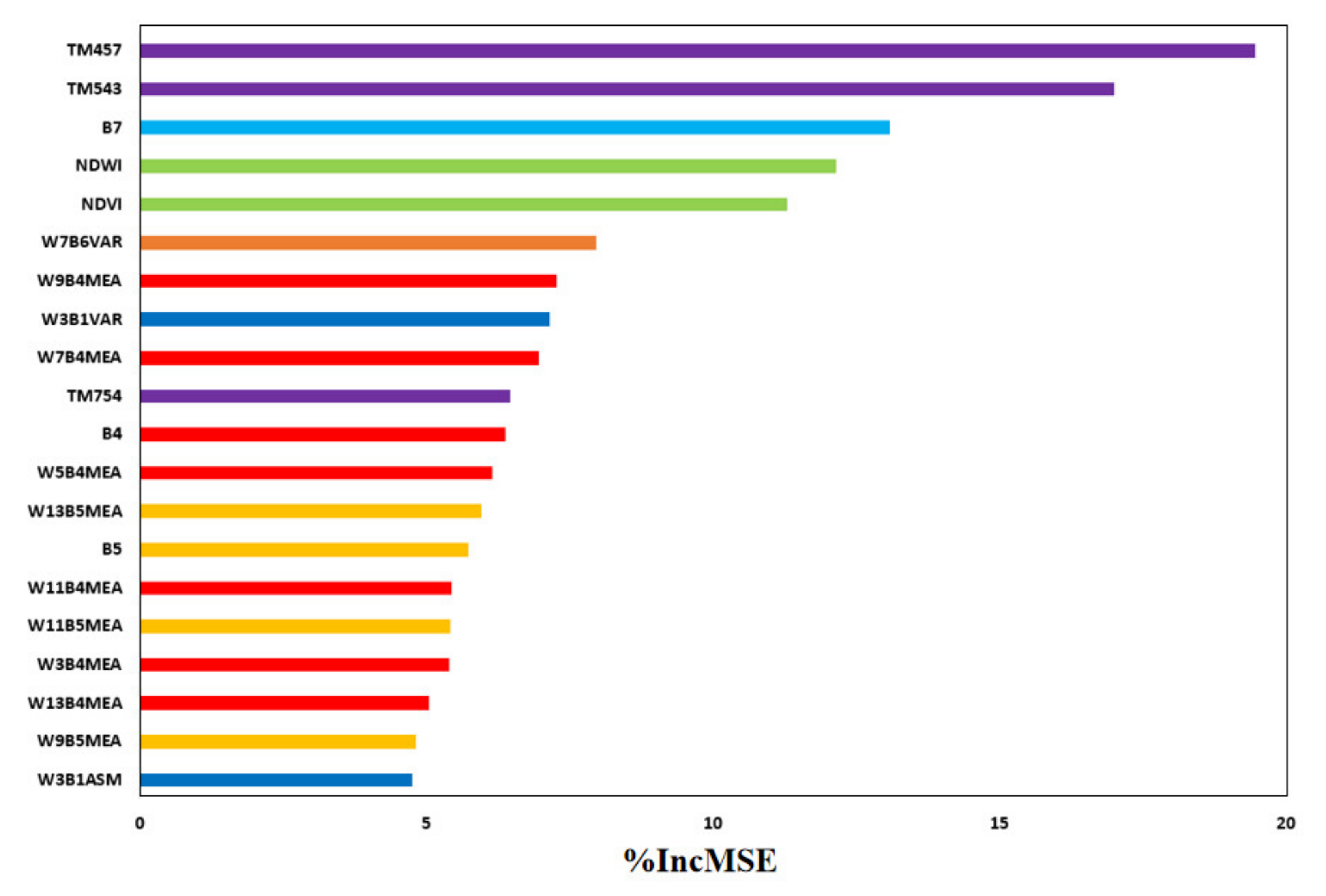
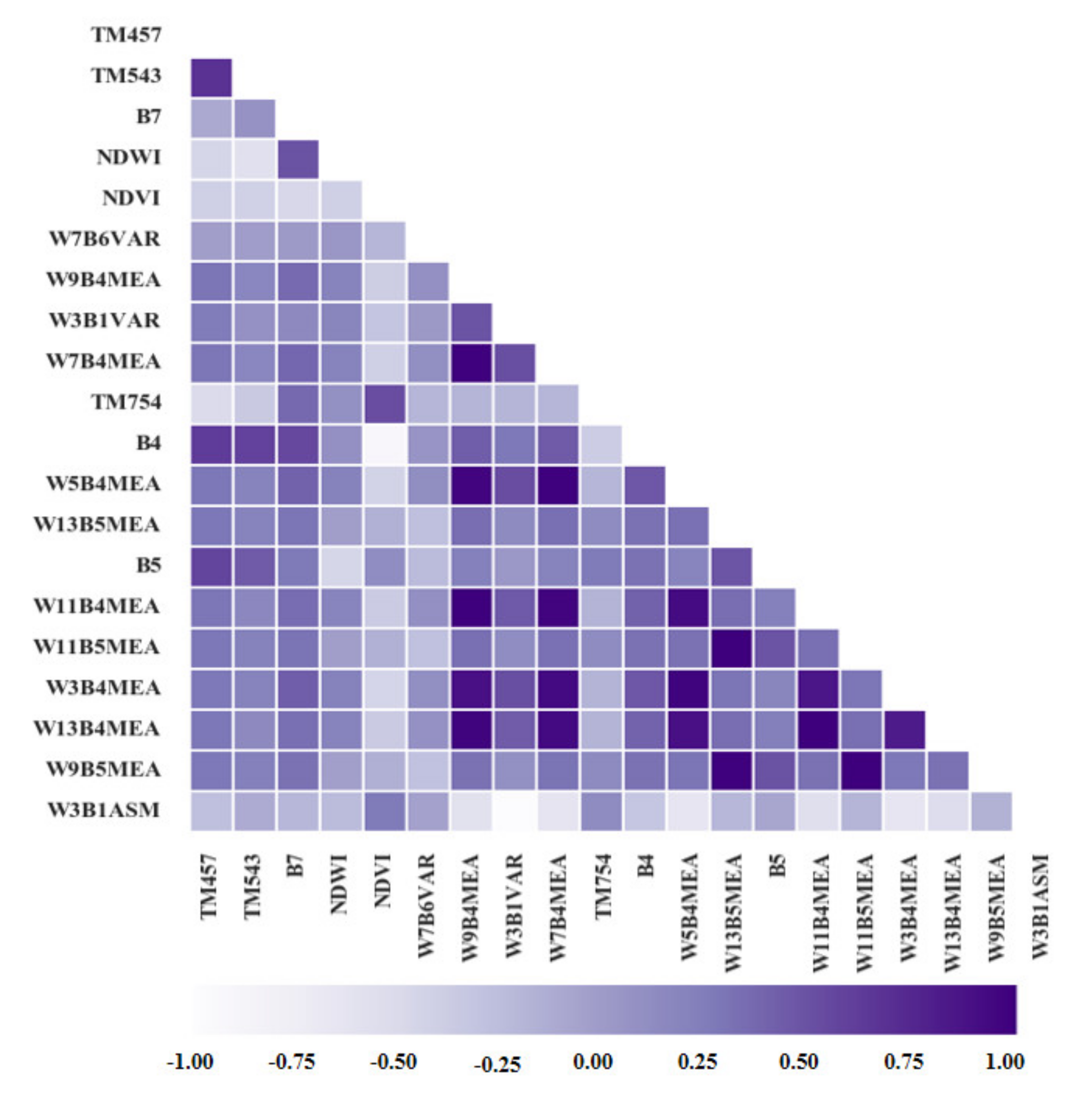
3.1. Selected Variables

The results of parameter optimization based on the RF model are shown in Figure 3. Figure 3a,b shows the influence of mtry and ntree, respectively, on the AGB simulation results of the RF model. Figure 3a shows that, when mtry was 203, the error of the model was the smallest. From Figure 3b, it can be seen that, when ntree reached approximately 2000, the model error tended to be stable. Therefore, in this study, the RF model parameter mtry was set to 203, ntree was set to 2000, and nodesize was set to 5 (by default). On this basis, the influence of the number of variables on the model error was further analyzed, as shown in Figure 3c. Figure 3c shows that the model error decreased rapidly with an increase in the number of variables. When the number of variables was more than six, the error rate of the model gradually increased. Therefore, considering the optimized RF model, when the number of variables was equal to six, the model error was the lowest.
Based on the optimized model, the importance of variables was screened. Figure 4 shows the importance scores of the top 20 variables after 100 runs of the RF model. As shown in Figure 4, the top six variables of the importance score were TM457, TM543, B7, NDWI, NDVI, and W7B6VAR. Combined with the analysis in Figure 3c, the six variables with the highest ranking in importance analysis were selected as the input variables for the GWR model.

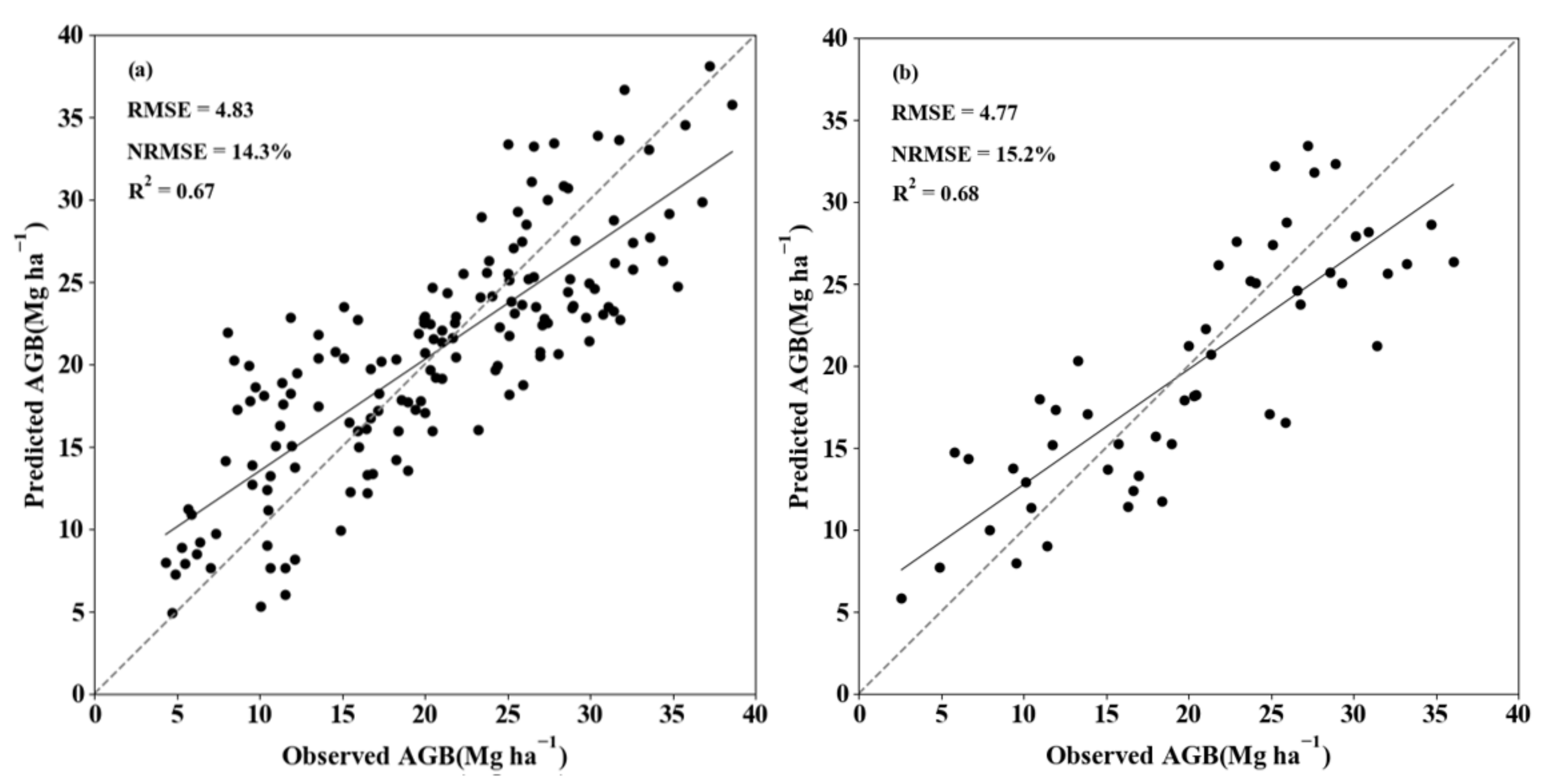
3.2. AGB Estimation Based on GWR

According to the GWR model, the bandwidth range in this study was 10–156 m. Figure 5 shows the impact of bandwidth on the AIC. As shown in Figure 5, the AIC decreased with increasing bandwidth, and the AIC value was the lowest when the bandwidth was 156 m. Therefore, the optimal bandwidth of the GWR model in this study was 156 m.
Based on the optimal bandwidth and the six selected variables, a GWR model for estimating the bamboo forest AGB in the study area was constructed. Figure 6 shows the spatial distribution of the regression parameters of the six variables in the model. Table 3 shows the descriptive statistics of the regression parameters. Figure 6 and Table 3 show that the parameters of different variables in the GWR model had obvious spatial differences. The parameters of B7, TM457, NDVI, and NDWI were larger in northwestern Zhejiang Province, while TM543 and W7B6VAR were larger in southern Zhejiang. This is the advantage of the GWR model; that is, considering the variation in the parameters across different spatial positions.
Figure 7a,b shows the fitting accuracy and verification accuracy analyses, respectively based on the GWR model. As shown in Figure 7, the fitting accuracy and validation accuracy (R2) of the GWR model were 0.73 and 0.74, respectively; the RMSE values were both 4.4 Mg ha−1; and the NRMSE values were 12.8% and 13.8%, respectively. This indicates that the GWR model constructed in this study can achieve the high-precision estimation of the bamboo forest AGB.

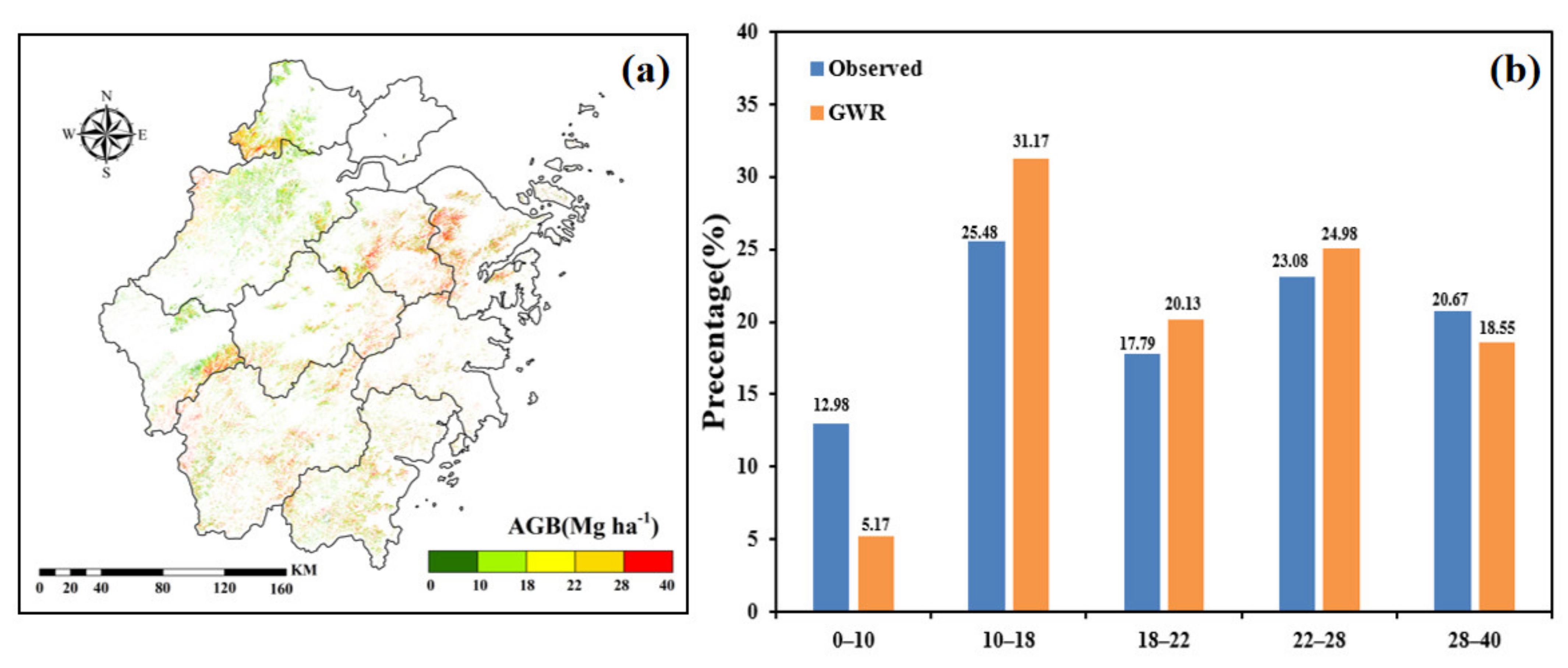
3.3. AGB Spatial Estimation of Bamboo Forest

Due to the high accuracy and low error of the GWR model, spatial estimation of the bamboo forest AGB in the study area was carried out based on the GWR model, as shown in Figure 8a. Figure 8a shows that most bamboo AGB in the study area was between 10 and 28 Mg ha−1, and the bamboo AGB in the northwest, southwest, and northeast was relatively dense.
To analyze the spatial distribution of bamboo AGB in the GWR model, we further compared the statistical histograms of the actual and estimated AGB, as shown in Figure 8b. From Figure 8b, it can be seen that the maximum proportion of bamboo AGB in Zhejiang was between 10 and 18 Mg ha−1, accounting for 31.17%, and the minimum proportion of bamboo AGB was between 0 and 10 Mg ha−1, accounting for 5.17% in the GWR model. The proportion of GWR results in 18–22 Mg ha−1, 22–28 Mg ha−1, and 28–40 Mg ha−1 were 20.13%, 24.98%, and 18.55%, respectively. The proportions were basically the same in 18–40 Mg ha−1; however, the proportion in the 0–10 Mg ha−1 region was underestimated, while the proportion in the 10–18 Mg ha−1 region was overestimated.

4. Discussion

To illustrate the advantages of the GWR model in the bamboo forest AGB estimation, we further constructed a COK model and an OLS-based multiple linear regression model.
For the estimation of COK, the bamboo forest AGB was used as the main variable, and the selected remote sensing variables were used as covariates. Then, out of the spherical model, exponential model, Gaussian model, J-Bessel model, and other variograms, J-Bessel was selected as the theoretical variogram (Table 4) based on the factors of high R2 and small residual. Finally, the bamboo forest AGB was estimated by the COK method. Figure 9a,b shows the fitting accuracy and verification accuracy analyses based on the COK model. As shown in Figure 9, the fitting accuracy and validation accuracy (R2) of the COK model were 0.67 and 0.68, respectively; the RMSE values were 4.83 Mg ha−1 and 4.77 Mg ha−1, respectively; and the NRMSE values were 14.3% and 15.2%, respectively.
Based on OLS, the multiple linear regression model constructed by TM457, TM543, B7, NDWI, NDVI, and W7B6VAR is shown in Formula (8):
AGB = 31.8192 + 0.002843 × B 7 0.005629 × TM 457 0.000362 × TM 543 + 11.5184 × NDVI + 19.4396 × NDWI 0.2196 × W 7 B 6 VAR
Figure 10a,b shows the fitting accuracy and verification accuracy analyses based on the OLS model. As shown in Figure 10, the fitting accuracy and validation accuracy (R2) of the OLS model were 0.65 and 0.66, respectively; the RMSE values were 5.06 Mg ha−1 and 5.13 Mg ha−1, respectively; and the NRMSE values were 14.5% and 15.5%, respectively.
The results indicate that the GWR model had the highest precision and strongest prediction ability, followed by the COK model, while the OLS model had the lowest precision. The prediction accuracy (R2) of the GWR model was 0.74, approximately 9% and 16% higher than the prediction accuracies of the COK and OLS models, respectively. The RMSE of the GWR model was only 4.4 Mg ha−1, approximately 7% and 12% lower than those of the COK and OLS models, respectively. The NRMSE of the GWR model was 13.8%, approximately 9% and 11% lower than those of the COK and OLS models, respectively. The GWR model had the highest accuracy, while the OLS model had the lowest accuracy. This may have been due to the following reasons.
First, the OLS model is a nonspatial regression model, while the GWR and COK models are both spatial models. According to Table 4, the structure ratios of various COK models were above 0.97; therefore, the bamboo forest AGB has strong spatial autocorrelation (i.e., the spatial distribution of AGB is nonrandom [47]). However, the OLS model is a completely stochastic model, and the spatial relationship of AGB is not considered in the estimation. Therefore, the GWR and COK models were found to be more suitable for spatial estimation of AGB, which was consistent with the research results of relevant scholars [48].
Second, although the GWR and OLS models are regression models, once the remote sensing information model based on OLS is constructed, the unified parameters are used to estimate the AGB pixel-by-pixel (Formula 4), ignoring the changes in model parameters in different spatial positions. The GWR model adds spatial relations (as weights) to the regression operation and calculates weights using a distance attenuation function, such that each of the remote sensing variables has different parameters in each pixel, as shown in Figure 6. This effectively reduces the spatial estimation error and ensures the accuracy of the results of AGB estimation.
Finally, as mentioned above, GWR and COK are both spatial models and, thus, have some advantages in AGB estimation. However, the COK model calculates the spatial autocorrelation scale based on a variogram (i.e., a range) and conducts spatial estimation within a limited range. The estimation accuracy of the model is closely related to the distribution of the sampling points. Generally, the closer to a sampling point, the smaller the estimation error of the model. However, the farther from a sampling point or in an area without sampling, the higher the estimation error of the model. The GWR model calculates the variable parameters of each point in the bandwidth based on existing sample data and the sample data within the bandwidth. The estimation results pay more attention to the local variation law, thus reducing the model error [48]. This may be the reason why the GWR model was better than the COK model, to some extent.
Bandwidth is key in the construction of the GWR model. Figure 11 shows the effect of bandwidth on model accuracy. As shown in Figure 11, when the bandwidth was very small, the training accuracy of the model was very high, but the prediction accuracy was very low. For instance, if the bandwidth was 10 m, the training accuracy (R2) was as high as 0.99, while the verification accuracy was only 0.1778. This is because the smaller bandwidth reduces the weight of the estimation points outside the bandwidth, which increases the model error. In this study, the AIC was used to calculate the optimal bandwidth of the GWR model, which was 156 m, thus ensuring the accuracy of AGB estimation.
In this study, the RF model was used to select six variables from 353 variables, including the original band, band combination, vegetation index, and GLCM texture features, to participate in the construction of the GWR model. Among them, the information of B5 variables accounted for 66.7% of the total variables, followed by the variable information based on B4 (with 50%). Figure 12 shows the correlation between the six selected variables and the bamboo forest AGB. Figure 12 shows that the six variables, especially TM457, TM543, and NDWI, had a significant correlation with the bamboo forest AGB. Therefore, the selection of remote sensing variables based on an RF model provided an important guarantee, enabling GWR to accurately estimate the bamboo forest AGB.
Figure 13 further analyzes the correlations of the top 20 variables of importance. From Figure 13, we can see that the weak correlations between variables indicate that the variables screened out by the RF can solve the multicollinearity problem in traditional statistical regression models to a great extent, thus laying an important foundation for the construction of the GWR and other models.

5. Conclusions

Based on Landsat 8 OLI imagery and AGB survey data of bamboo forests in Zhejiang Province, we established a GWR model to estimate the bamboo forest AGB in Zhejiang Province and compared the estimation results with COK and traditional OLS-based multiple linear regression models. The results showed that TM457, TM543, B7, NDWI, NDVI, and W7B6VAR greatly contributed to AGB estimation. The GWR model based on these variables had high precision and strong prediction ability, followed by the COK model, while the OLS model had the lowest precision. Among them, the prediction accuracy (R2) of the GWR model was 0.74, which was 9% and 16% higher than the prediction accuracies of the COK and OLS models, respectively. The error (RMSE) of the GWR model was 7% and 12% lower than the errors of the COK and OLS models, respectively, and its NRMSE was 9% and 11% lower than those of the COK and OLS models, respectively. The optimal bandwidth of the GWR model was 156 m. The parameters of different variables in the GWR model had obvious spatial differences. The parameters B7, TM457, NDVI, and NDWI were larger in northwestern Zhejiang Province, while the parameters TM543 and W7B6VAR were larger in southern Zhejiang Province. This is the advantage of the GWR model, considering the change in parameters at different spatial positions. Based on the GWR model, most of the bamboo forest AGB in Zhejiang Province ranged from 10 to 32 Mg ha−1, mainly distributed in the northwest, southwest, and northeast parts of the province. This is in line with the actual bamboo forest AGB distribution in Zhejiang Province, indicating the potential practical value of our study.

Author Contributions

Conceptualization, H.D.; Data curation, J.W., X.L., J.J. and F.K.; Formal analysis, J.W., X.L., F.M., M.Z. and E.L.; Funding acquisition, H.D.; Investigation, J.W.; Methodology, J.W.; Project administration, H.D.; Software, J.W.; Validation, J.W.; Visualization, J.W.; Writing—original draft preparation, J.W.; Writing—review and editing, H.D.. All authors have read and agreed to the published version of the manuscript.

Funding

The authors gratefully acknowledge the support of the National Natural Science Foundation of China (Nos. 31670644, 31901310), the State Key Laboratory of Subtropical Silviculture (No. ZY20180201), and Zhejiang Provincial Collaborative Innovation Center for Bamboo Resources and High-efficiency Utilization (Grant No. S2017011). The Key Research and Development Program of Zhejiang Province (2021C02005).

Institutional Review Board Statement

Not applicable.

Informed Consent Statement

Not applicable.

Data Availability Statement

Landsat 8 OLI satellite data comes from Geospatial Data Cloud (http://www.gscloud.cn/), last access 20 July 2021.

Acknowledgments

The authors gratefully acknowledge the supports of various foundations. The authors are grateful to the editor and anonymous reviewers whose comments have contributed to improving the quality of this study.

Conflicts of Interest

The authors declare that they have no competing interests.

References

  1. Nichol, J.E.; Sarker, M.L.R. Improved biomass estimation using the texture parameters of two high-resolution optical sensors. IEEE Trans. Geosci. Remote Sens. 2011, 49, 930–948. [Google Scholar] [CrossRef] [Green Version]
  2. Dong, L.; Du, H.; Han, N.; Li, X.; He, S. Application of Convolutional Neural Network on Lei Bamboo Above-Ground-Biomass (AGB) Estimation Using Worldview-2. Remote Sens. 2020, 12, 958. [Google Scholar] [CrossRef] [Green Version]
  3. Xu, X.; Du, H.; Zhou, G.; Fan, W. Review on Correlation Analysis of Independent Variables in Estimation Models of Vegetation Biomass Based on Remote Sensing. Remote Sens. Technol. Appl. 2008, 23, 239–247. [Google Scholar]
  4. Brown, S. Aboveground biomass estimates for tropical moist forests of Brazilian Amazon. Interciencia 1992, 17, 8–18. [Google Scholar]
  5. Fang, J.Y. Forest Biomass of China: An estimate based on the Biomass-Volume Relationship. Ecol. Appl. 1998, 8, 1084–1091. [Google Scholar]
  6. Fang, J.Y. Forest biomass estimation at regional and global levels, with special reference to China’s forest biomass. Ecol. Res. 2010, 16, 587–592. [Google Scholar] [CrossRef]
  7. Li, D.; Wang, C.; Hu, Y.; Liu, S. General Review on Remote Sensing-Based Biomass Estimation. Geomat. Inf. Sci. Wuhan Univ. 2012, 37, 631–635. [Google Scholar]
  8. Wang, C.; Jia, X.; Zhao, Y.; Jin, H.; Liu, L.; Yin, H.; Wang, Z. Review of Methods on Estimation Forest Biomass. J. Beihua Univ. (Nat. Sci.) 2019, 20, 116–119. [Google Scholar]
  9. Zhu, X.; Liu, D. Improving forest aboveground biomass estimation using seasonal Landsat NDVI time-series. Isprs J. Photogramm. Remote Sens. 2015, 102, 222–231. [Google Scholar] [CrossRef]
  10. Tian, X.; Yan, M.; van der Tol, C.; Li, Z.; Su, Z.; Chen, E.; Li, X.; Li, L.; Wang, X.; Pan, X.; et al. Modeling forest above-ground biomass dynamics using multi-source data and incorporated models: A case study over the qilian mountains. Agric. For. Meteorol. 2017, 246, 1–14. [Google Scholar] [CrossRef]
  11. Sasan, V.; Javad, S.; Kamran, A.; Hadi, F.; Hamed, N.; Tien, P.; Dieu, T.B. Improving Accuracy Estimation of Forest Aboveground Biomass Based on Incorporation of ALOS-2 PALSAR-2 and Sentinel-2A Imagery and Machine Learning: A Case Study of the Hyrcanian Forest Area (Iran). Remote Sens. 2018, 10, 172. [Google Scholar]
  12. Ojoatre, S.; Zhang, C.; Hussin, Y.; Kloosterman, H.; Ismail, M.H. Assessing the Uncertainty of Tree Height and Aboveground Biomass From Terrestrial Laser Scanner and Hypsometer Using Airborne LiDAR Data in Tropical Rainforests. IEEE J. Sel. Top. Appl. Earth Obs. Remote Sens. 2019, 12, 4149–4159. [Google Scholar] [CrossRef] [Green Version]
  13. Zhang, R.; Zhou, X.; Ouyang, Z.; Avitabile, V.; Giannico, V. Estimating aboveground biomass in subtropical forests of China by integrating multisource remote sensing and ground data. Remote Sens. Environ. 2019, 232, 111341. [Google Scholar] [CrossRef]
  14. Puliti, S.; Breidenbach, J.; Schumacher, J.; Hauglin, M.; Astrup, R. Above-ground biomass change estimation using national forest inventory data with Sentinel-2 and Landsat 8. arXiv 2020, arXiv:2010.14262. [Google Scholar]
  15. Huaqiang, D.U.; Zhou, G.; Hongli, G.E.; Fan, W.; Xiaojun, X.U.; Fan, W.; Shi, Y. Satellite-based carbon stock estimation for bamboo forest with a non-linear partial least square regression technique. Int. J. Remote Sens. 2012, 33, 1917–1933. [Google Scholar]
  16. Duan, Z.; Zhao, D.; Zeng, Y.; Zhao, Y.; Wu, B.; Zhu, J. Estimation of the Forest Aboveground Biomass at Regional Scale Based on Remote Sensing. Geomat. Inf. Sci. Wuhan Univ. 2015, 40, 1400–1408. [Google Scholar]
  17. Li, Y.; Ning, H.; Li, X.; Du, H.; Xing, L. Spatiotemporal Estimation of Bamboo Forest Aboveground Carbon Storage Based on Landsat Data in Zhejiang, China. Remote Sens. 2018, 10, 898. [Google Scholar] [CrossRef] [Green Version]
  18. Li, X.; Du, H.; Mao, F.; Zhou, G.; Chen, L.; Xing, L.; Fan, W.; Xu, X.; Liu, Y.; Cui, L. Estimating bamboo forest aboveground biomass using EnKF-assimilated MODIS LAI spatiotemporal data and machine learning algorithms—ScienceDirect. Agric. For. Meteorol. 2018, 256–257, 445–457. [Google Scholar] [CrossRef]
  19. Rasel, S.; Chang, H.C.; Ralph, T.J.; Saintilan, N.; Diti, I.J. Application of feature selection methods and machine learning algorithms for saltmarsh biomass estimation using Worldview-2 imagery. Geocarto Int. 2019, 1–25. [Google Scholar] [CrossRef]
  20. Zhang, M.; Du, H.; Zhou, G.; Li, X.; He, S. Estimating Forest Aboveground Carbon Storage in Hang-Jia-Hu Using Landsat TM/OLI Data and Random Forest Model. Forests 2019, 10, 1004. [Google Scholar] [CrossRef] [Green Version]
  21. He, P.; Zhang, H.; Lei, X.; Xu, G.; Gao, X. Estimation of Forest Above-Ground Biomass Based on Geostatistics. Sci. Silvae Sin. 2013, 49, 101–109. [Google Scholar]
  22. Guo, H. Geographically Weighted Regression based Estimation of Regional Forest Carbon Storage; Zhejiang A&F Universuty: Hangzhou, China, 2015. [Google Scholar]
  23. Zhou, L.; Ou, G.; Wang, J.; Xu, H. Light Saturation Point Determination and Biomass Remote Sensing Estimation of Pinus kesiya var. langbianensis Forest Based on Spatial Regression Models. Sci. Silvae Sin. 2020, 56, 38–47. [Google Scholar]
  24. Izadi, s.; Sohrabi, H. Estimating the Spatial Distribution of Above-ground Carbon of Zagros Forests using Regression Kriging, Geographically Weighted Regression Kriging and Landsat 8 imagery. J. Environ. Sci. Technol. 2020. [Google Scholar] [CrossRef]
  25. Izadi, S.; Sohrabi, H.; Jafari Khaledi, M. Comparison of Geographically Weighted Regression and Regression Kriging to Estimate the Spatial Distribution of Aboveground Biomass of Zagros Forests. J. Geomat. Sci. Technol. 2020, 9, 113–124. [Google Scholar]
  26. Zhang, B.; Ou, G. Application of Spatial Effect and Regression Model on Forestry Research. J. Southwest For. Univ. 2016, 144–152. [Google Scholar]
  27. Zhang, L.; Shi, H. Local Modeling of Tree Growth by Geographically Weighted Regression. Forest Sci. 2004, 50, 225–244. [Google Scholar]
  28. Foody, G.M. Geographical weighting as a further refinement to regression modelling: An example focused on the NDVI–rainfall relationship. Remote Sens. Environ. 2003, 88, 283–293. [Google Scholar] [CrossRef]
  29. Kupfer, J.A.; Farris, C.A. Incorporating spatial non-stationarity of regression coefficients into predictive vegetation models. Landsc. Ecol. 2006, 22, 837–852. [Google Scholar]
  30. Fotheringham, A.S.; Brunsdon, M. Spatial Variations in School Performance: A Local Analysis Using Geographically Weighted Regression. Geogr. Environ. Model. 2001, 5, 43–66. [Google Scholar] [CrossRef]
  31. Dong, L.; Xing, L.; Liu, T.; Du, H.; Zhang, M. Very High Resolution Remote Sensing Imagery Classification Using a Fusion of Random Forest and Deep Learning Technique—Subtropical Area for Example. IEEE J. Sel. Top. Appl. Earth Obs. Remote Sens. 2019, 13, 113–128. [Google Scholar] [CrossRef]
  32. Tian, Q.; Zheng, L. Image-Based atmospheric radiation correction and reflectance retrieval methods. Q. J. Appl. Meteorol. 1998, 9, 456–461. [Google Scholar]
  33. Kaufman, Y.J.; Tanré, D. Strategy for direct and indirect methods for correcting the aerosol effect on remote sensing: From AVHRR to EOS-MODIS. Remote Sens. Environ. 1996, 55, 65–79. [Google Scholar] [CrossRef]
  34. Tang, J.; Nie, Z. Geometric Correction of Remote Sensing Image. Geomat. Spat. Inf. Technol. 2007, 30, 100–102. [Google Scholar]
  35. Zhou, G. Carbon Storage, Fixation and Distribution in Mao Bamboo(Phyllostachys Pubescens) Stands Ecosystem. Ph.D. Thesis, Zhejiang University, Hangzhou, China, 2006. [Google Scholar]
  36. Tian, Q.; Min, X. Advances in study on vegetation indices. Adv. Earth Sci. 1998, 13, 327–333. [Google Scholar]
  37. Richardson, A.J.; Wiegand, C.L. Distinguishing vegetation from soil background information. Photogramm. Eng. Remote Sens. 1977, 43, 1541–1552. [Google Scholar]
  38. Kaufman, Y.J.; Tanre, D.; Holben, B.N.; Markham, B.; Gitelson, A. Atmospheric effects on the NDVI—Strategies for its removal. In Proceedings of the International Geoscience & Remote Sensing Symposium, Houston, TX, USA, 26–29 May 1992; IEEE: Piscataway, NJ, USA, 1992. [Google Scholar]
  39. McFeeters, S.K. The use of the Normalized Difference Water Index (NDWI) in the delineation of open water features. Int. J. Remote Sens. 1996, 17, 1425–1432. [Google Scholar] [CrossRef]
  40. Haralick, R.M. Statistical and structural approaches to texture. Proc. IEEE 2005, 67, 786–804. [Google Scholar] [CrossRef]
  41. Sun, Y.; Wang, W.; Li, G. Spatial distribution of forest carbon storage in Maoershan region, Northeast China based on geographically weighted regression kriging model. Chin. J. Appl. Ecol. 2019, 30, 1642–1650. [Google Scholar]
  42. Lv, Y.; Li, C.; Ou, G.; Xiong, H.; Wei, A.; Zhang, B.; Xu, H. Remote Sensing Estimation of Biomass of Pinus kesiya var. langbianensis by Geographically Weighted Regression Models. For. Resour. Manag. 2017. [Google Scholar] [CrossRef]
  43. Akaike, H.T. A new look at the statistical model identification. Autom. Control IEEE Trans. 1974, 19, 716–723. [Google Scholar] [CrossRef]
  44. Liu, C. Spatial Distribution of Forest Carbon Storage in Heilongjiang Province. Ying Yong Sheng Tai Xue Bao 2014, 25, 2779–2786. [Google Scholar]
  45. Han, N.; Du, H.; Zhou, G.; Xiaojun, X.; Cui, R.; Gu, C. Spatiotemporal heterogeneity of Moso bamboo aboveground carbon storage with Landsat Thematic Mapper images: A case study from Anji County, China. Int. J. Remote Sens 2013, 34, 4917–4932. [Google Scholar] [CrossRef]
  46. Wang, H.; Hou, R.; Zheng, D.; Gao, X.; Xia, C.; Peng, D. Biomass Estimation of Arbor Forest in Subtropical Region Based on Geographically Weighted Regression Model. Trans. Chin. Soc. Agric. Mach. 2018, 49, 184–190. [Google Scholar]
  47. Propastin, P. Modifying geographically weighted regression for estimating aboveground biomass in tropical rainforests by multispectral remote sensing data. Int. J. Appl. Earth Obs. Geoinf. 2012, 18, 82–90. [Google Scholar] [CrossRef]
  48. Du, H.; Zhou, G.; Fan, W.; Ge, H.; Fan, W. Spatial heterogeneity and carbon contribution of aboveground biomass of moso bamboo by using geostatistical theory. Plant Ecol. 2010, 207, 131–139. [Google Scholar] [CrossRef]
Figure 1. (a) Location of the study area; (b) distribution and biomass of bamboo forests in Zhejiang Province in 2014; (c) 2014 Landsat 8 false-color synthesis image of Zhejiang Province.
Remotesensing 13 02962 g001
Figure 2. Flowchart of steps used in our study for comparison of different algorithms and variables for bamboo forest AGB estimation.
Remotesensing 13 02962 g002
Figure 3. (a) Influence of mtry on model error (Mg ha−1); (b) influence of ntree on model error (Mg ha−1); (c) influence of the number of variables on model error (Mg ha−1).
Remotesensing 13 02962 g003
Figure 4. Importance of the top 20 variables (in terms of percentage increase of mean square error). WiBjxxx indicates GLCM texture xxx based on band j with window size i × i. (e.g., W7B6VAR indicates the sixth band’s variance with a window size of 7 × 7).
Remotesensing 13 02962 g004
Figure 5. Selection of optimal bandwidth for the GWR model.
Remotesensing 13 02962 g005
Figure 6. Spatial distribution of model coefficients for different variables in the GWR model.
Remotesensing 13 02962 g006
Figure 7. Comparison between observed and predicted AGB by the GWR model with (a) training samples and (b) testing samples.
Remotesensing 13 02962 g007
Figure 8. (a) The GWR model inversion of AGB in Zhejiang Province in 2014 and (b) percentage of spatial variation of AGB observed in sample plots and the percentage of spatial variation of the bamboo forest AGB estimated by the GWR models.
Remotesensing 13 02962 g008
Figure 9. Comparison of observed and predicted AGB by the COK model with (a) training samples and (b) testing samples.
Remotesensing 13 02962 g009
Figure 10. Comparison of observed and predicted AGB by the OLS model with (a) training samples and (b) testing samples.
Remotesensing 13 02962 g010
Figure 11. Influence of bandwidth selection on accuracy.
Remotesensing 13 02962 g011
Figure 12. Correlation between selected variables and bamboo forest AGB.
Remotesensing 13 02962 g012
Figure 13. Autocorrelation of the top 20 variables.
Remotesensing 13 02962 g013
Table 1. Landsat 8 OLI image information of Zhejiang.
Data IdentificationRow/Column NumberDateCloudage
LC81180392014164LGN00118,03913 June 201410.03
LC81180402014164LGN00118,04013 June 20146.05
LC81180412014164LGN00118,04113 June 20147.94
LC81190392014203LGN00119,03922 July 20142.31
LC81190402014203LGN01119,04022 July 20143.09
LC81190412014203LGN00119,04122 July 20144.02
LC81200392014162LGN01120,03911 June 20141.03
LC81200402014162LGN01120,04011 June 20140.09
Table 2. The used variables and formulations of variables.
TypeNameDetailsReferences
BandsBand 1 Coastal (B1)/
Band 2 Blue (B2)/
Band 3 Green (B3)/
Band 4 Red (B4)/
Band 5 NIR (B5)/
Band 6 SWIR 1 (B6)/
Band 7 SWIR 2 (B7)/
Band CombinationsTM754 B 7 × B 5 / B 4 [17]
TM563 B 5 × B 6 / B 3
TM457 B 4 × B 5 / B 7
TM432 B 4 × B 3 / B 2 .
TM543 B 5 × B 4 / B 3
Vegetation IndicesDifference Vegetation Index (DVI) B 5 B 4 [37]
Normalized Difference Vegetation Index (NDVI) B 5 B 4 / B 5 + B 4 [38]
Normalized Difference Water Index (NDWI) B 3 B 5 / B 3 + B 5 [39]
Ratio Vegetation Index (RVI) B 5 / B 4 (Pearson, 1972)
Solid-Adjusted Vegetation Index (SAVI) 1.5 × B 5 B 4 / B 5 + B 4 + 0.5 (Huete, 1988)
Gray-Level Co-Occurrence MatricesMean (MEA) M E A = i , j = 0 N 1 i P i , j [40]
Variance (VAR) V A R = i , j = 0 N 1 P i , j 1 μ i
Homogeneity (HOM) H O M = i , j = 0 N 1 i P i , j 1 + i j 2
Contrast (CON) C O N = i , j = 0 N 1 i P i , j i j
Dissimilarity (DIS) D I S = i , j = 0 N 1 i P i , j i j
Entropy (ENT) E N T = i , j = 0 N 1 P i , j ln P i , j
Augular Second Moment (ASM) A S M = i , j = 0 N 1 i P i , j 2
Correlation (COR) C O R = i , j = 0 N 1 i i , j N 1 i j P i , j μ i μ j σ i 2 σ j 2
Notes: μ i = i = 0 N 1 i j = 0 N 1 P i , j
σ i = j = 0 N 1 i μ i 2 j = 0 N 1 P i , j
Table 3. Descriptive statistics of the local regression parameters of the GWR model.
VariablesMinMaxMeanStdDev
Intercept29.88707636.21116132.8304431.933700
TM457−0.006452−0.005701−0.0061290.000224
TM543−0.000883−0.000303−0.0005640.000188
B70.0021190.0045650.0034070.000633
NDWI12.254419.260516.5377752.102416
NDVI6.1357510.8158.0276861.299880
W7B6VAR−0.5350640.396925−0.0783340.282045
Table 4. Optimal variance function model and parameters fitted by the COK model.
ModelR2Residual SSNuggetStillStructural RatioRange
Spherical0.67113384.700.03121.17890.97357978.455
Exponential0.67593460.670.01021.15690.99118989.212
Gaussian0.56893734.110.00121.19050.98698373.171
Rational Quadratic0.67713371.190.00111.10920.9997983.505
Hole Effect0.68093551.670.02211.0180.97827983.505
K-Bessel0.68073291.640.00831.08110.999839,449.225
J-Bessel0.68263275.970.02171.09260.9810,357.08
Publisher’s Note: MDPI stays neutral with regard to jurisdictional claims in published maps and institutional affiliations.

