1. Introduction
In recent decades, Global Navigation Satellite System (GNSS) have made great progress, including Global Positioning System (GPS) modernization by the USA, the BeiDou Navigation Satellite System (BDS) developed by China, the Galileo Navigation Satellite System (Galileo) constructed by the European Union (UN), the Global Navigation Satellite System in Russia (GLONASS) restored by Russia, and the Quasi-Zenith Satellite System (QZSS) implemented by Japan, which have realized interoperability and multifrequency signal support [
1,
2,
3,
4,
5]. The Galileo system operated by the European Space Agency (ESA) supports all satellite broadcasts of E1 (1575.42 MHz), E5a (1176.45 MHz), E5b (1207.14 MHz), E5 (1191.795 MHz) and E6 (1278.75 MHz) five-frequency signals throughout the constellation to provide positioning, navigation, and timing (PNT) services worldwide [
6,
7]. Galileo multifrequency signals have improved capacity redundancy and reliability, have provided more opportunities in low-noise combination, cycle-slip detection, and repair [
8,
9], ambiguity resolution [
10], positioning [
7,
11], time-frequency transfer [
12] and other aspects, and have faced more challenges of inter frequency bias (
IFB), which represents significant development potential.
With the support of the precise ephemeris and clock products provided by IGS Analysis Centers (ACs), precise point positioning (PPP) technology has gradually become a popular research topic due to its characteristics of high precision and flexible operation and has been widely used in the field of geosciences and time-frequency transfer [
13,
14]. The PPP technique has been adopted by the Bureau International des Poids et Mesures (BIPM) and many other international laboratories for international atomic time (TAI) maintenance applications since 2009 [
15,
16].
Many scholars have investigated the performance of Galileo multifrequency signals in positioning, timing, and orbit determination. Duong et al. [
17] proved the multifrequency advantage of PPP ambiguity resolution (AR) and found that the four-frequency Galileo combination of E1/E5a/E5b/E6 provides the lowest geometric and ambiguity variance. Tu et al. [
18] studied the performance of real-time kinematics (RTK) using Galileo four-frequency observations, and the results showed that multiple frequencies were much better than single-frequency, and the coordinates’ standard deviation (STD) was improved by approximately 30%. Liu et al. [
19] proposed the method of PPP uncombined (UC) AR by using Galileo triple-frequency observations. Qin et al. [
20] investigated Galileo precise time transfer with the COM (which denotes precise satellite orbit and clock bias products provided by Center for Orbit Determination in Europe (CODE)), WUM (which denotes precise satellite orbit and clock bias products provided by Wuhan University (WHU)), GRM (which denotes multi GNSS precise satellite orbit and clock bias products provided by Centre National d’Etudes Spatiales (CNES)), SHA (which denotes precise satellite orbit and clock bias products provided by Shanghai Astronomical Observatory (SHAO)), and GBM (which denotes precise satellite orbit and clock bias products provided by Geo Forschungs Zentrum (GFZ)) final products and CLK93 (which denotes real-time (RT) precise satellite orbit and clock bias products provided by CNES) RT products. Li et al. [
21] proved the superiority of the Galileo five-frequency signal in PPP rapid ambiguity solutions compared with dual-frequency and triple-frequency solutions. Zhang et al. [
22] focused on the Galileo quad-frequency PPP time and transfer performance with E1, E5a, E5b and E5 observations. Liu et al. [
23] used the phase bias product provided by CNES to test triple-frequency GPS/Galileo RT PPP AR and proved that triple-frequency PPP AR can improve the convergence time performance and positioning accuracy compared with dual-frequency PPP AR. Kuang et al. [
24] studied RT UC orbit determination using Galileo triple-frequency observations and the characteristics of satellite inter frequency clock bias (IFCB). Su and Jin [
25] analyzed the receiver clock, tropospheric delay, receiver IFBs and differential code bias (
DCB) of combined and UC five-frequency PPP models and proved the consistency of several models.
Jin and Su [
26] presented and evaluated PPP models using the single-, dual-, triple-, and quad-frequency BDS observations, and the results show that the multi-frequency BDS observations will greatly improve the PPP performances. Ge et al. [
27] proved that quad-frequency BDS-3 or Galileo PPP models could be used to time transfer, the stability and accuracy of quad-frequency and dual-frequency
IF model are the same.
Previous studies focused more on Galileo dual-frequency (DF), triple-frequency (TF) and quad-frequency (QF) precise positioning but less on five-frequency (FF) precise positioning and precise time-frequency transfer. The contribution of this work is that we established multiple
IF and UC PPP mathematical models with Galileo five frequency observations, and provided the processing method and specific formula of
IFB parameters in the multi-frequency PPP model. In addition, based on the evaluation the multipath combination noise of Galileo multi-frequency observations, the convergence time and positioning accuracy of DF, TF, QF and FF models were evaluated by using precision products of different ACs, and the performance of time-frequency transfer of Galileo E1, E5a, E5b, E5 and E6 multi frequency signals is compared and analyzed systematically for the first time. In
Section 2, five mathematical PPP models of the Galileo E1, E5a, E5b, E5 and E6 frequency observations are established; observation types, combination coefficients, ionospheric coefficients and noise amplification coefficients of the Galileo DF, TF, QF, and FF PPP models are also summarized and compared.
Section 3 introduces the experimental data and their processing strategy. In
Section 4, we use the GBM, WUM and GRG (which denote precise satellite orbit and clock bias products provided by the Centre National d’Etudes Spatiales (CNES)) precise products to evaluate the positioning and the time-frequency transfer performance results of the Galileo DF, TF, QF, and FF PPP models. Finally, we summarize this work and draw some conclusions.
2. Methodology
In this section, starting from GNSS raw observations, the Galileo FF UC PPP model, the single ionosphere-free (IF) PPP model among five frequency observations, two QF IF PPP model among five frequency observations, three TF IF PPP model among five frequency observations and four DF IF PPP model among five frequency observations are established, respectively. Then, the observation types, combination coefficients, ionospheric coefficients and noise amplification coefficients of the Galileo DF, TF, QF, and FF PPP models are summarized and compared.
2.1. GNSS Observation Model
GNSS pseudo range and carrier phase observations can be expressed as [
28]:
where the
P and
L denote pseudo range and carrier phase observation values in meters, respectively; superscript
i denotes the
i-th satellite of the GNSS system; subscripts
r and
j denote the receiver and frequency identifiers, respectively; for convenience, the frequency identifiers 1, 2, 3, 4 and 5 in the Galileo system represent E1, E5a, E5b, E5 and E6 frequencies, respectively;
λ is wavelength corresponding to frequency
j;
ρ represents the geometric distance between the satellite and receiver;
c represents the speed of light in a vacuum;
dtr and
dts denote receiver and satellite clock offsets in seconds, respectively;
MF denotes the wet mapping function;
ZWD is zenith troposphere wet delay (
ZWD);
I denotes the slant ionospheric delay;
denotes frequency dependent ionospheric delay amplification factors,
;
N is carrier phase integer ambiguity;
d denotes the receiver uncalibrated code delay (UCD) in meters;
b denotes uncalibrated phase delay (UPD) in cycles; and
ζ and
ξ represent the pseudo orange and carrier phase observation noises, respectively.
Defining the notations:
where
and
are
IF combination frequency factors (
m,
n = 1, 2, 3, 4, 5;
m ≠
n).
2.2. Five-Frequency UC PPP Model
In the five-frequency UC PPP model, the ionospheric delay is related to E1/E5a
IF combined with
DCB and cannot be separated, and the
IFB parameters are required to compensate for the inconsistency of receiver UCDs at the E5b, E5 and E6 frequencies. Then, the Galileo five-frequency UC pseudo range and carrier phase observations can be expressed as:
with
where
p and
l are pseudo range and carrier phase observed minus computed (OMC) values in meters, respectively; subscript
IF denotes ionospheric-free combination;
DCBr,12 denotes E1 and E5a
DCB of the receiver side;
IFBuc denotes UC IFBs;
μ denotes the unit vector of the component from the receiver to the satellites;
x denotes the vector of the receiver position increments; and hat “~” denotes the reparametrized estimate.
2.3. Single Five-Frequency IF Combination (FF1) PPP Model
Galileo five-frequency observations can be combined according to the geometry-free, ionospheric-free and minimum noise principles with a single ionospheric combination observation and can be expressed as:
The coefficients following the above criteria can be uniquely determined as [
25]:
with
where
e1,
e2,
e3,
e4 and
e5 denote the five-frequency
IF combination coefficients,
e is the coefficient in the denominator.
When the five pseudo range measurements are combined within a single equation, the FF1 PPP observation equation can be expressed as:
with
where the receiver clock offset will absorb the UCD of E1/E5a/E5b/E5/E6
IF combination.
2.4. Two Quad-Frequency IF Combinations (FF2) PPP Model
In the FF2 PPP model, E1/E5a/E5b/E5 and E1/E5a/E5b/E6 observations were selected to form two quad-frequency
IF combinations. Similarly, additional
IFB parameters were required to maintain compatibility between the two quad-frequency
IF combinations. Hence, the two quad-frequency
IF combination PPP models can be formulated as follows:
with
where
IFBIF1235 denotes the
IFB parameters between the E1/E5a/E5b/E6 and E1/E5a/E5b/E6 code
IF combinations.
2.5. Three Triple-Frequency IF Combinations (FF3) PPP Model
The FF3 PPP model for the Galileo five-frequency was implemented by combining the three triple-frequency
IF observations, and we chose E1/E5a/E5b, E1/E5a/E5 and E1/E5a/E6 observations for combination. In this case, we needed to add two estimated
IFB parameters, which can be expressed as:
with
where
IFBIF124 and
IFBIF125 denote the
IFB parameters between the E1/E5a/E5b, E1/E5a/E6 and E1/E5a/E5b code
IF combinations.
2.6. Four Dual-Frequency IF Combinations (FF4) PPP Model
The FF4 PPP model consists of the observation equation implemented by combining the four DF
IF observations. Theoretically, any two Galileo E1, E5a, E5b, E5, and E6 signals can form a dual-frequency ionospheric-free combination. However, considering the noise amplification coefficients after combination, we chose E1/E5a, E1/E5b, E1/E5 and E1/E6 signals for combination. In addition, it was necessary to note that the clock difference of each combination is not consistent. In this case, we needed to add estimated
IFB parameters, which can be expressed as:
with
where
IFBIF13,
IFBIF14 and
IFBIF15 denote the
IFB parameters between the E1/E5b, E1/E5, E1/E6 and E1/E5a code
IF combinations.
2.7. Comparison of Galileo Five Frequency PPP Models
Table 1 summarizes the types of observation values, combination coefficients, ionospheric delay coefficients and noise amplification coefficients of the dual-frequency, triple-frequency, quad-frequency, and five-frequency PPP models. Among them, the FF2, FF3 and FF4 PPP models are composed of DF, TF and QF
IF combinations, and additional
IFB parameters need to be estimated to maintain consistency among different equations. The noise amplification factor of FF1 is smaller than that of other
IF combinations. After the filter converges and the ionosphere and ambiguity parameters are separated, the FF1, FF2, FF3, FF4 and UC PPP models are equivalent.
2.8. Date Selection and Processing Strategies
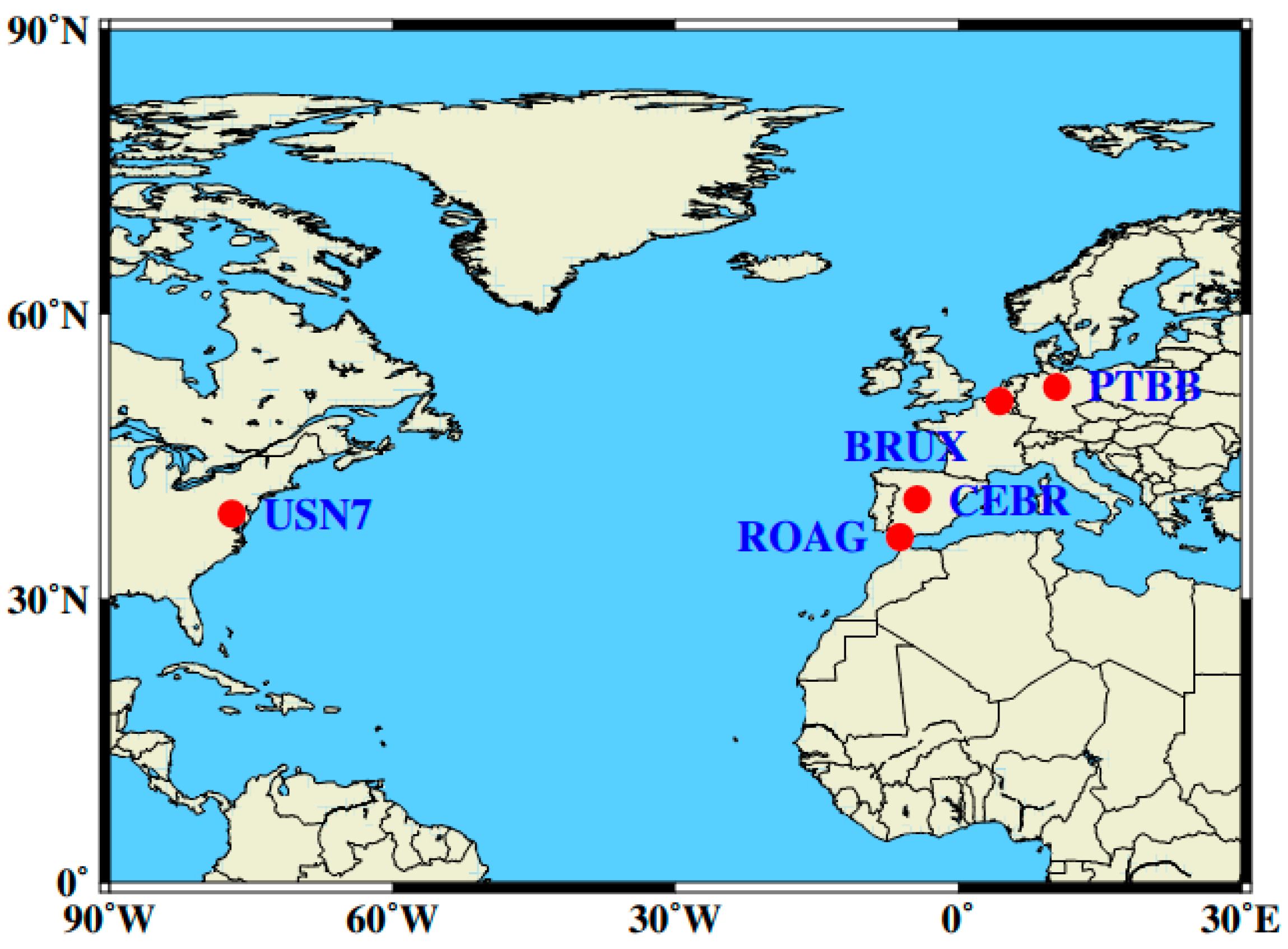
Five stations that can receive the Galileo E1/E5a/E5b/E5/E6 signal observations over a period of 190–196 days in 2020 were selected from the international GNSS service (IGS) multi-GNSS experiment (MGEX) network. In order to ensure the reliability of time-frequency transfer, the stations of UTC (Coordinated Universal Time) laboratories were preferred in our research. The sampling interval of the observations was 30 s. These stations were all equipped with high-precision atomic clocks. With the BRUX station as the reference station, four time-frequency links ranging from 454.6 km to 5591.2 km were established.
Figure 1 shows the distribution of the selected MGEX stations, the information of which is listed in
Table 2.
The code and phase observation noises were set to 0.3 m and 3.0 mm, respectively, and elevation-dependent weighting for the observations was applied. Since the receiver phase center offset (PCO) and phase center variation (PCV) corrections for Galileo were not available, we used the GPS signal corrections for Galileo signals. Such a strategy has been used effectively by various authors [
29,
30]. In addition, for the E5b, E5, and E6 observables, receiver PCO and PCV corrections for the GPS L2 frequency were used. Since different observations were used in the same satellite clock estimation, there were IFCBs in the E5b, E5 and E6 observations [
31]. Relevant research shows that the consistency of Galileo multifrequency time-dependent UCDs can be ensured; thus, IFCBs in the Galileo system can be neglected [
30]. The detailed processing strategies are summarized in
Table 3.
3. Results
First, we evaluated the number of visible satellites, time dilution of precision (TDOP) and multipath noises of BRUX, CEBR, PTBB, ROAG and USN7 stations with Galileo satellites. Then, the positioning performances and time-frequency transfer stabilities of four models (DF, TF, QF and FF1) composed of dual-frequency, triple-frequency, quad-frequency, and five-frequency observations were compared by PPP solution; the positioning accuracies, IFB parameters and time-frequency transfer stabilities of the five-frequency observation models (FF1, FF2, FF2, FF3, FF4 and UC) were also evaluated. Finally, we used different AC precise products to compare and evaluate the performances of different PPP models. It should be noted that the positioning performance was assessed with respect to the coordinates from the IGS SNX file, and the principle of convergence was that the three-dimensional (3D) bias of twenty successive epochs is better than 10.0 cm; in addition, the 3D root mean square (RMS) values after convergence were counted. The modified Allan deviation (MADEV) was used as the stability index of time-frequency transfer.
3.1. Number of Visible Satellites, TDOP and Multipath Combination Noise Analysis
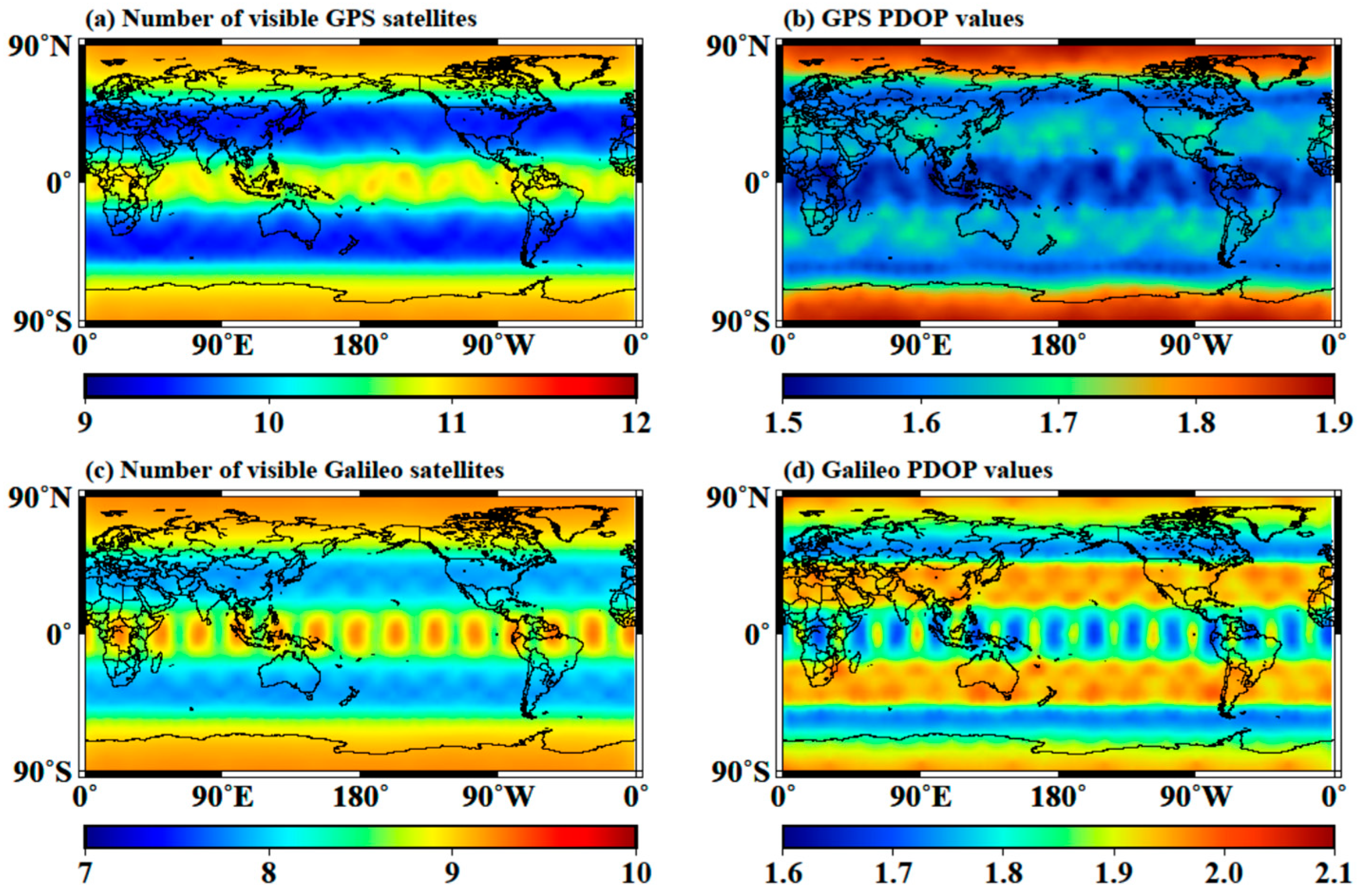
Until July 2020, the Galileo system had twenty-four valid satellites in orbit, including four in-orbit validation (IOV) satellites and twenty fully operational capability (FOC) satellites. The distribution of the average number of visible satellites and average position dilution of precision (PDOP) values for the GPS and Galileo constellations with a cutoff elevation of 5.0 degrees with a 1° × 1° grid on days of year (DOYs) 190 to 196 in 2020 are shown in
Figure 2.
As shown in
Figure 2, the number of visible satellites and the PDOP value of the GPS and Galileo constellations are symmetrically distributed with the equator, which shows a strong correlation with the dimension, and the positioning performance is better near the equator; the average number of visible satellites of Galileo ranges from 7.0 to 10.0, and the average PDOP value of Galileo ranges from 1.6 to 2.1. By comparison, the average number of visible satellites of Galileo is slightly less than that of GPS, and the PDOP value of Galileo is slightly larger than that of GPS.
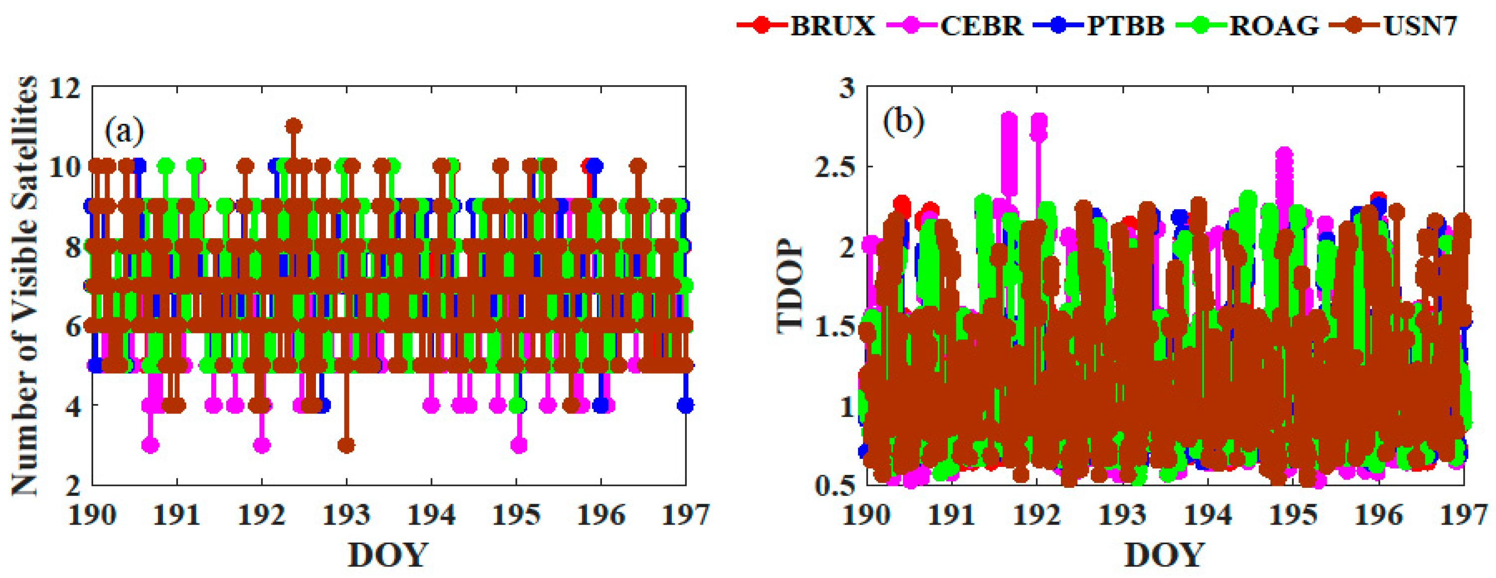
Figure 3 presents the number of visible satellites and TDOP values of the five stations. When the cutoff satellite elevation is 7 degrees, the average numbers of visible satellites at stations BRUX, CEBR, PTBB, ROAG and USN7 are 7.08, 6.6, 7.05, 6.68 and 8.85, respectively. Among them, the number of visible satellites with gross error removed at some moments of CEBR and USN7 stations are less than 4.0, which cannot be a PPP solution. It can be observed from the right figure that the TDOP values of the five stations all have some noise phenomenon, which will affect the accuracy of the time-frequency transfer of this epoch. The average TDOPs of the BRUX, CEBR, PTBB, ROAG and USN7 stations are 1.12, 1.29, 1.14, 1.26 and 1.26, respectively.
As shown in
Figure 4, the multipath combination noise of each frequency is within ± 2.0 m, among which the multipath combination noise of the E1 frequency is the largest and that of the E5 frequency is the smallest. When the cutoff elevation is 7 degrees, the BRUX station E1, E5a, E6, E5 and E5b multipath combination noise RMS values are 0.224 m, 0.166 m, 0.190 m, 0.116 m and 0.198 m, respectively; the CEBR station E1, E5a, E6, E5 and E5b multipath combination noise RMS values are 0.319 m, 0.305 m, 0.350 m, 0.144 m and 0.312 m, respectively; the PTBB station E1, E5a, E6, E5 and E5b multipath combination noise RMS values are 0.311 m, 0.209 m, 0.243 m, 0.161 m and 0.247 m, respectively; the ROAG station E1, E5a, E6, E5 and E5b multipath combination noise RMS value are 0.166 m, 0.126 m 0.148 m, 0.083 m, and 0.149 m, respectively; and the USN7 station E1, E5a, E6, E5 and E5b multipath combination noise RMS values are 0.378 m, 0.307 m, 0.355 m, 0.130 m and 0.331 m, respectively. It is obvious that the multipath combination noise of the CEBR station and USN7 station is the largest and that of the ROAG station is the smallest.
3.2. Performance of the DF, TF, QF and FF1 PPP Models
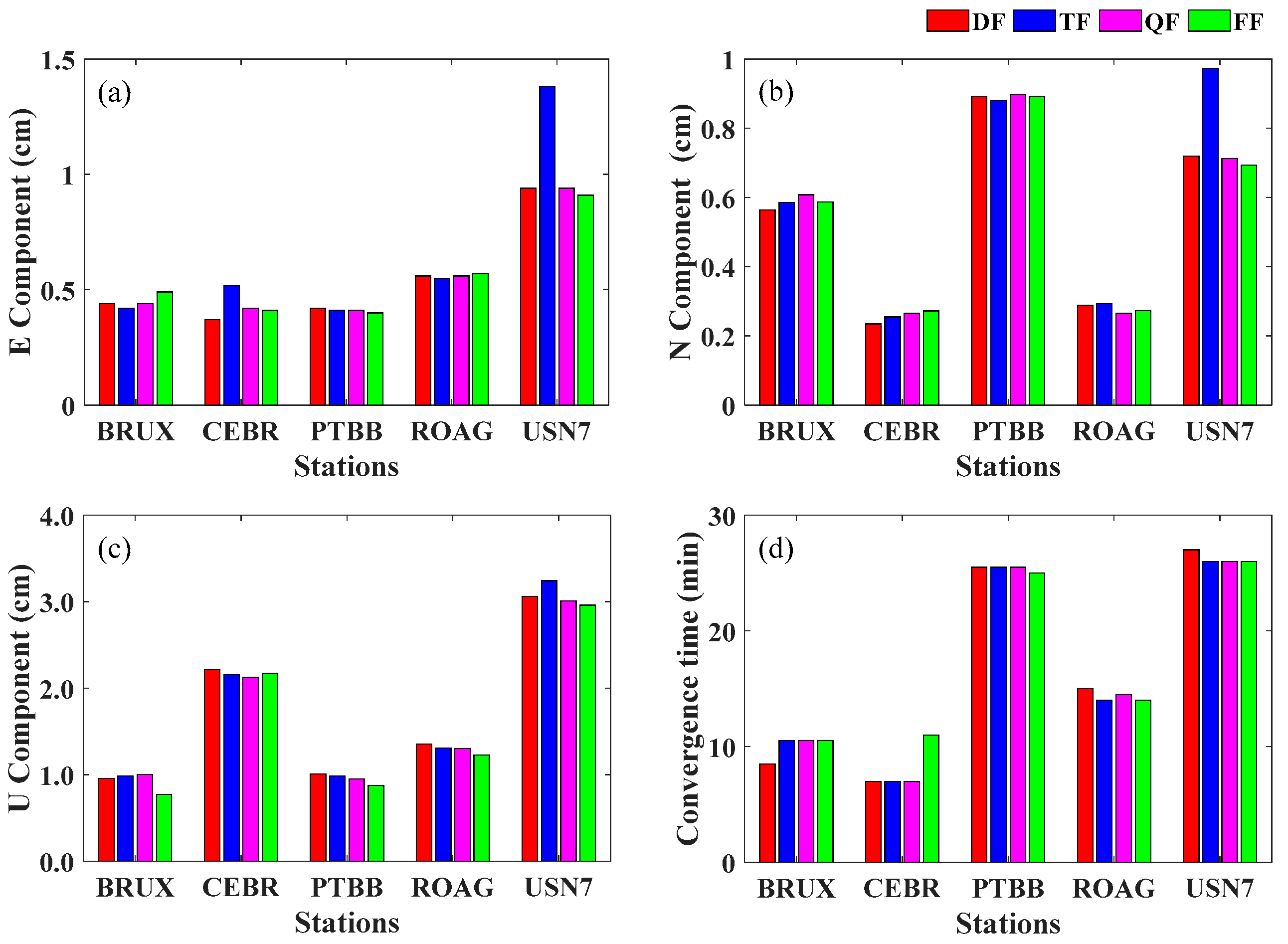
As shown in
Figure 5, the positioning RMS values and convergence times of the DF, TF, QF and FF1 PPP models are close to each other. With the increasing of the frequency, the positioning performance has no obvious improvement, and some stations have even weakened. Among them, the PPP performance of station USN7 is obviously weaker than that of the other stations, especially the E and N components, which have large changes in the TF PPP model. The convergence times of the BRUX, CEBR and ROAG stations are less than 15.0 min, and those of the PTBB and USN7 stations are approximately 25.0 min. According to the statistics, the average 3D RMS values of the DF, TF, QF and FF1 PPP models are 1.88 cm, 1.95 cm, 1.85 cm, and 1.78 cm, respectively; the average convergence times are 16.6 min, 16.6 min, 16.7 min and 17.3 min, respectively.
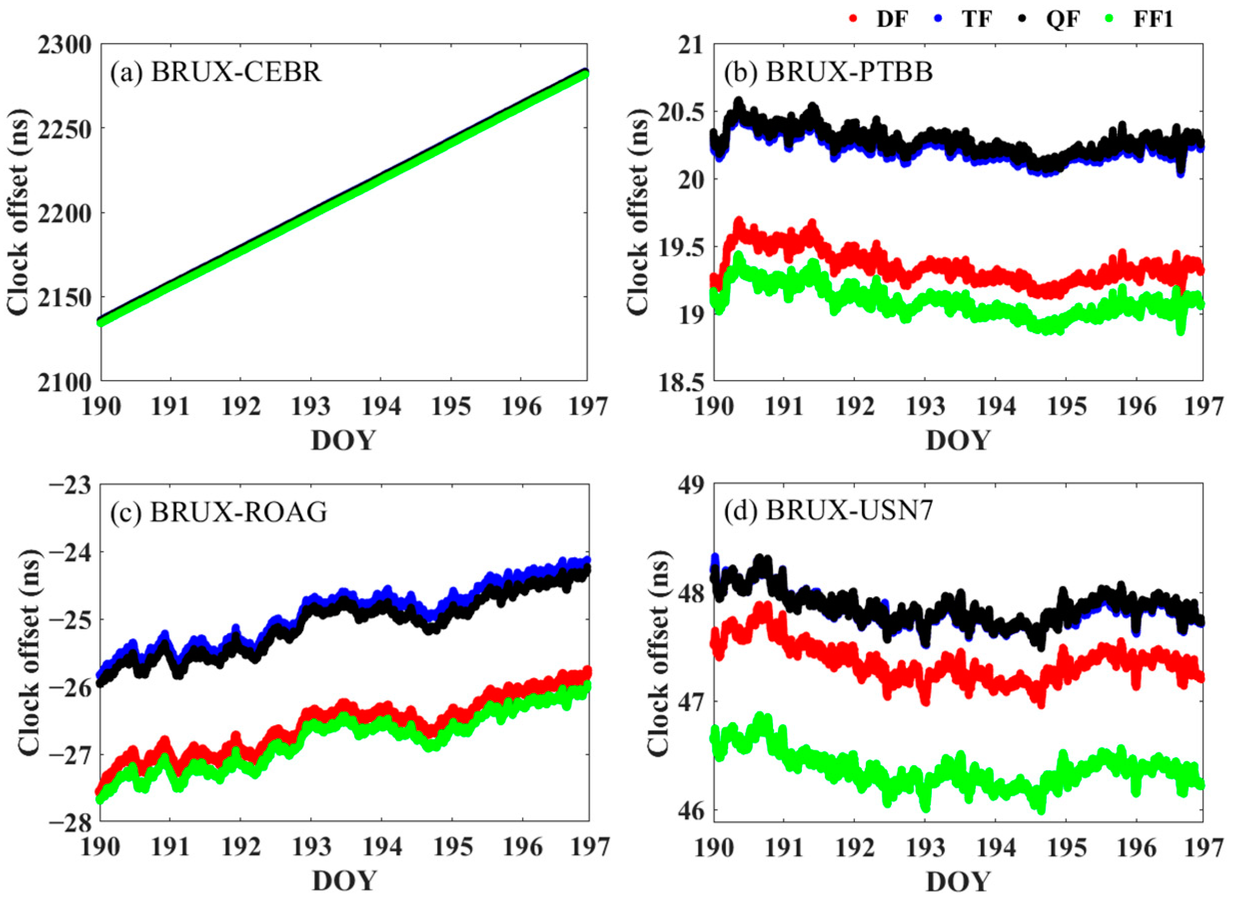
The clock offset sequences of the DF, TF, QF and FF1 PPP models are shown in
Figure 6. Due to the influence of
IFB parameters, the clock offsets of the various PPP models show a certain deviation, and the deviations of the TF and QF models are minimal. The RMS deviations between the TF, QF, FF1 and DF PPP models of the BRUX-CEBR link are 0.30 ns, 0.06 ns and 1.46 ns, respectively; the RMS deviations between the TF, QF, FF1 and DF PPP models of the BRUX-PTBB link are 0.89 ns, 0.93 ns and 0.26 ns, respectively; the RMS deviations between the TF, QF, FF1 and DF PPP models of the BRUX-ROAG link are 1.66 ns, 1.50 ns and 0.21 ns, respectively; and the RMS deviations between the TF, QF, FF1 and DF PPP models of the BRUX-USN7 link are 0.49 ns, 0.50 ns and 0.99 ns, respectively.
As shown in
Table 4, the average values among the four time-frequency links in each model are completely consistent, and the RMS values have only slight deviations, which indicates that the multifrequency stability is not significantly improved compared with the dual-frequency stability. The RMS value of the inter-epoch difference of the BRUX-CEBR link is approximately 10.5 ps, and those of the other three time-frequency links are less than 8.2 ps, which indicates that the frequency stability of the BRUX-CEBR link is worse. In addition, it is noted that the hydrogen atomic clock attached to the BRUX-CEBR link has obvious clock drift, which is related to the performance of the CEBR station atomic clock.
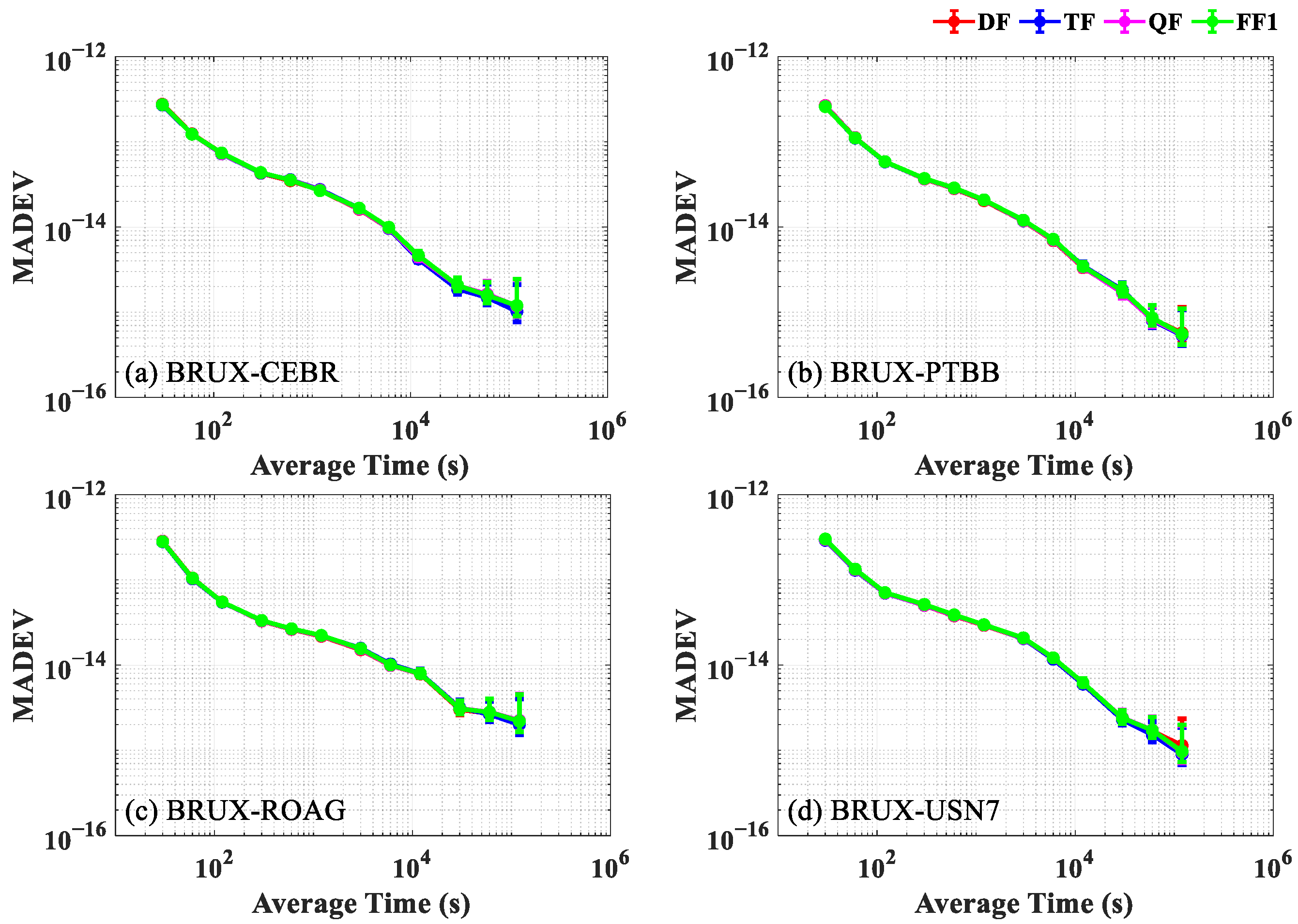
Figure 7 presents a comparison of the frequency stabilities for the DF, TF, QF and FF1 PPP models, which are generally identical for different solutions at the four time-frequency links. The frequency stability of the BRUX-PTBB link reaches the 10
−16 level in 60,000 s and 5.31 × 10
−16 in 120,000 s, the BRUX-USN7 link reaches 9.25 × 10
−16 in 120,000 s, and those of the other two links are also close to the 10
−16 level in 120,000 s. The average frequency stabilities at 120,000 s for the four time-frequency links surpass 1.23 × 10
−15 for the DF PPP model, 1.15 × 10
−15 for the TF PPP model, 1.23 × 10
−15 for the QF PPP model and 1.23 × 10
−15 for the FF1 PPP model.
3.3. Performance of the FF1, FF2, FF3, FF4 and UC PPP Models
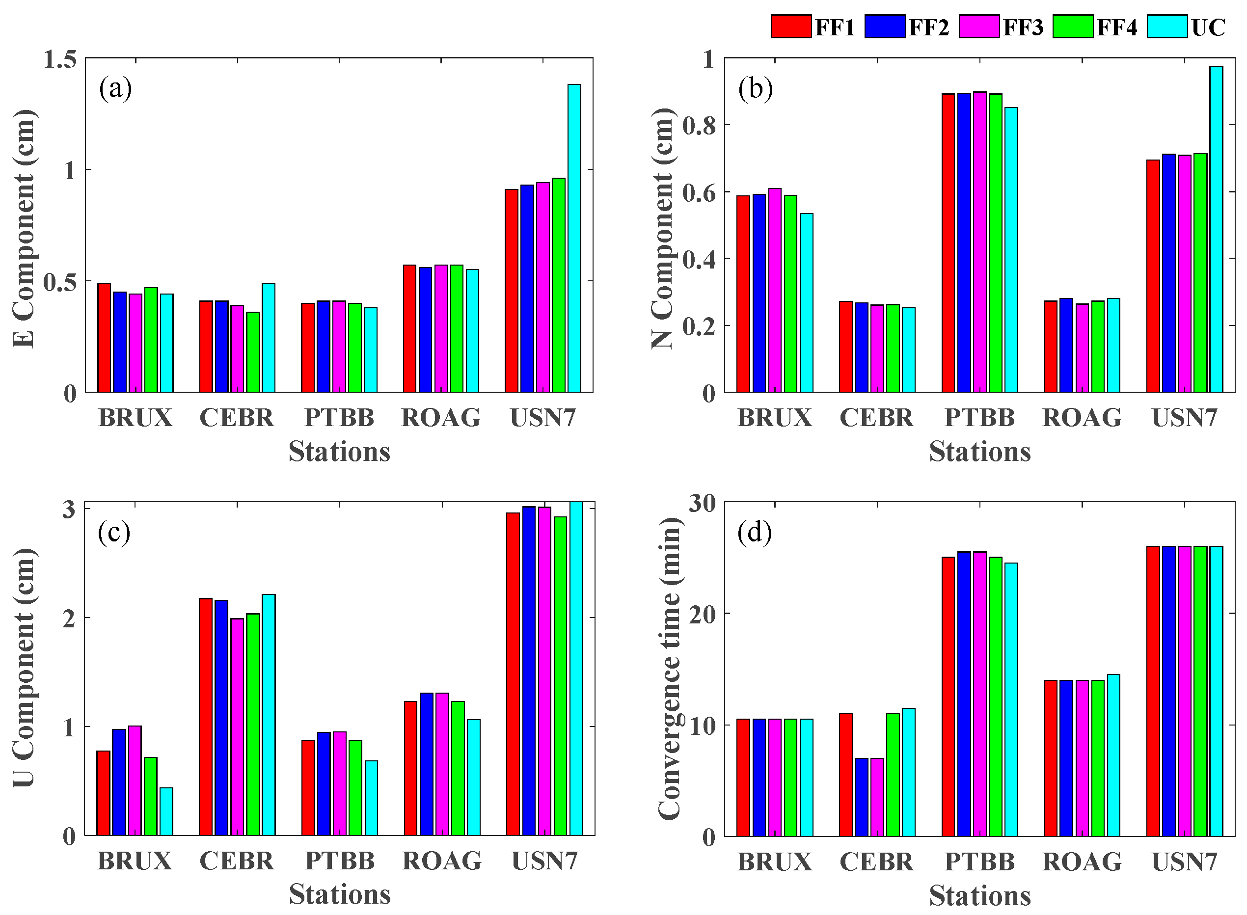
Figure 8 presents the positioning performances of the FF1, FF2, FF3, FF4 and UC PPP models. The positioning performances of several Galileo five-frequency PPP models are basically the same, but USN7 station E and U component RMS values by UC PPP are slightly worse. According to the statistics, the average 3D RMS values of the DF, TF, QF and FF1 PPP models are 1.78 cm, 1.85 cm, 1.82 cm, 1.74 cm, and 1.73 cm, respectively; and the average convergence times are 17.3 min, 16.6 min, 16.6 min, 17.3 min, and 17.4 min, respectively.
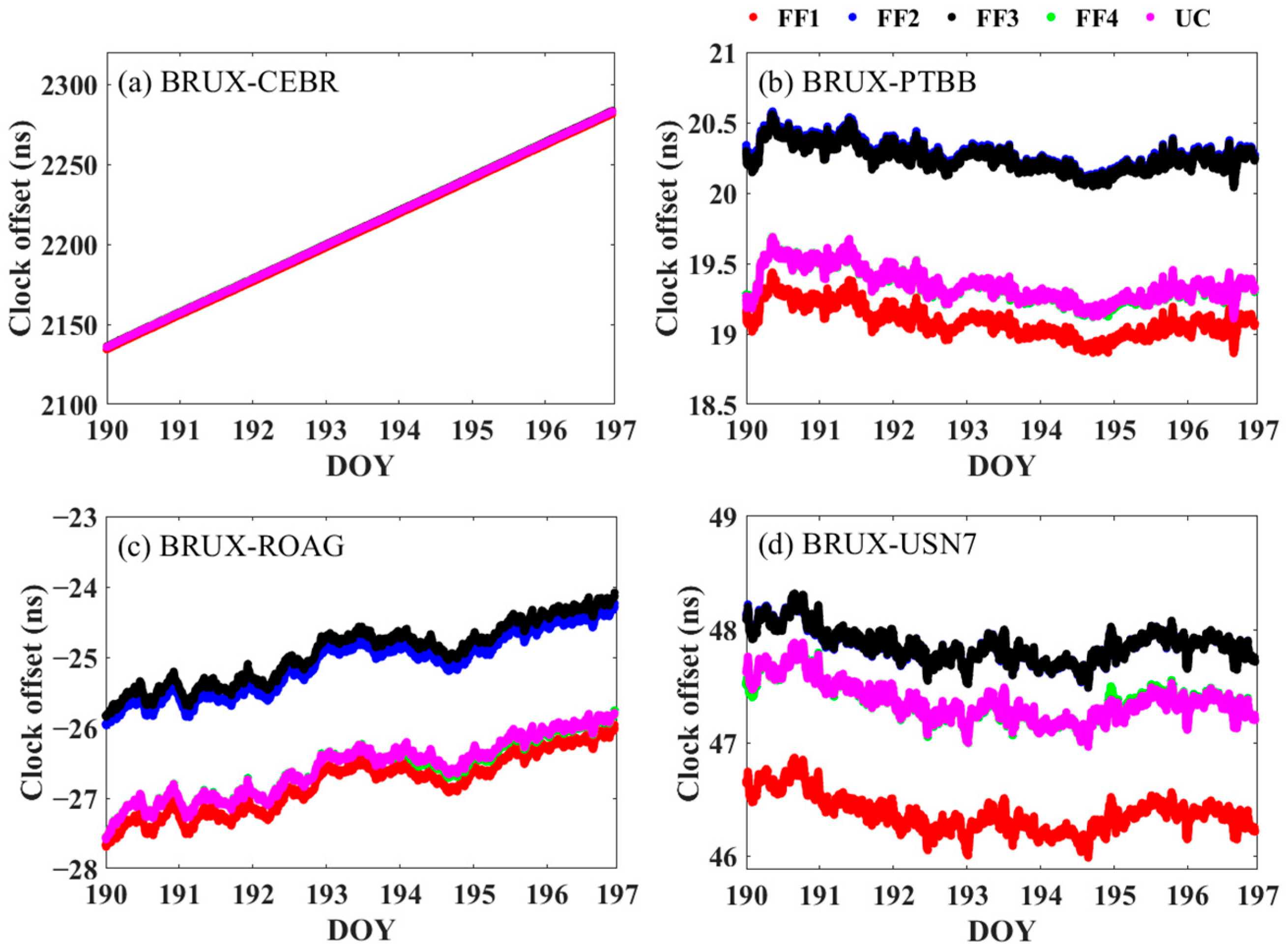
Figure 9 presents the clock offsets of five-frequency PPP models, and each clock offset sequence has the same trend, which proves the correctness of the algorithm. In addition, there are some deviations among the clock offsets, among which the FF1 and FF2 PPP models and the FF4 and UC PPP models have minimum deviations. Based on the clock offset of the FF1 model, the RMS values of FF2, FF3, FF4 and UC compared with FF1 in the BRUX-CEBR link are 1.56 ns, 1.86 ns, 1.49 ns and 1.44 ns, respectively; the RMS values of the FF2, FF3, FF4 and UC PPP models compared with the FF1 PPP model in the BRUX-PTBB link are 1.17 ns, 1.15 ns, 0.25 ns and 0.25 ns, respectively; the RMS values of FF2, FF3, FF4 and UC compared with FF1 in the BRUX-ROAG link are 1.71 ns, 1.87 ns, 1.49 ns and 0.23 ns, respectively; and the RMS values of FF2, FF3, FF4 and UC compared with FF1 in the BRUX-ROAG link are 1.51 ns, 1.01 ns and 1.01 ns, respectively.
As shown in
Table 5, the average RMS values of the BRUX-CEBR, BRUX-PTBB, BRUX-ROAG and BRUX-USN7 time-frequency links are 10.48 ps, 6.90 ps, 7.11 ps and 8.09 ps, respectively; and the average RMS values of the FF1, FF2, FF3, FF4 and UC models are 8.16 ps, 8.16 ps, 8.17 ps, 8.08 ps and 8.16 ps, respectively. It is worth noting that although in the UC model, one needs to estimate the ionospheric delay since the receiver clock bias is easily affected by the unmodeled ionospheric delay, the AVG and RMS of the UC model are still close to those of the
IF PPP models.
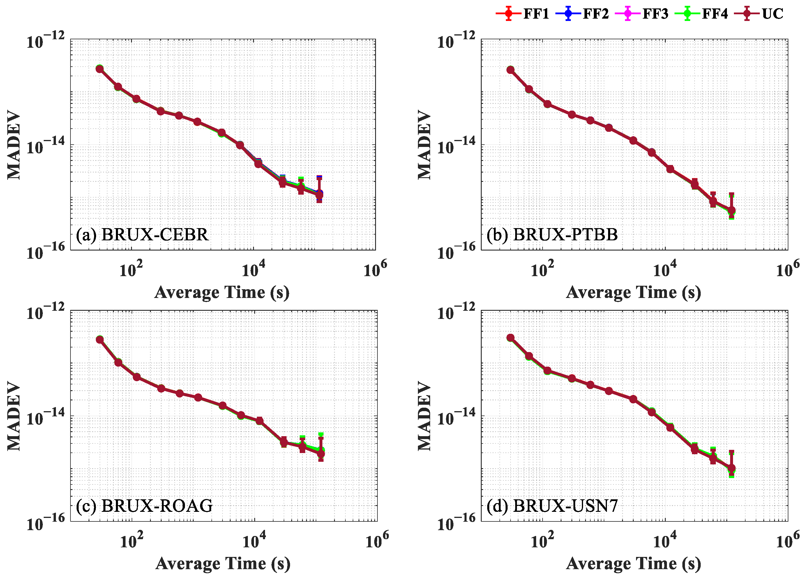
Figure 10 presents comparisons of the MADEVs for the FF1, FF2, FF3, FF4 and UC PPP models. The MADEVs of the PPP models with different five-frequency combinations are basically the same. The average frequency stabilities at 120,000 s for four time-frequency links surpassed 1.23 × 10
−15 for the FF1 PPP model, 1.22 × 10
−15 for the FF2 PPP model, 1.20 × 10
−15 for the FF3 PPP model and 1.24 × 10
−15 for the UC PPP model.
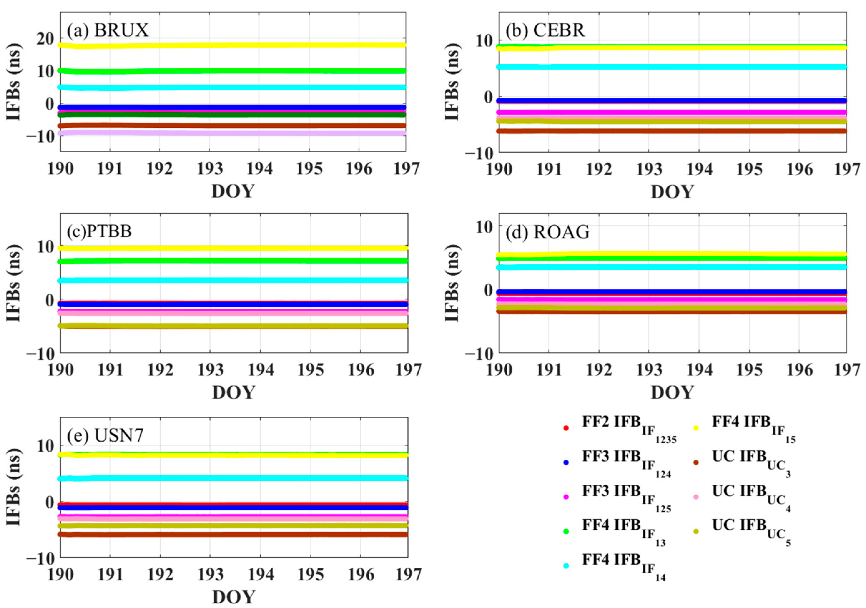
As shown in
Figure 11, the
IFB sequences are basically stable, and the
IFB values of the FF4 model are the largest. The average RMS values of
IFBIF13,
IFBIF14, and
IFBIF15 in the FF4 PPP model are 7.8 ns, 4.1 ns, and 9.9 ns, respectively; and the average STD values are 0.04 ns, 0.03 ns, and 0.15 ns, respectively. The average RMS values of
IFBUC3,
IFBUC4, and
IFBUC5 in the UC PPP model are 5.49 ns, 3.09 ns, and 5.15 ns, respectively, and the corresponding average STD values are 0.03 ns, 0.02 ns, and 0.04 ns, respectively. As mentioned, the
IFBIF15 STD value of the FF4 PPP model is the largest, leading to the receiver clock bias, and
IFBIF15 cannot be accurately separated, which will affect the time-frequency transfer performance.
3.4. PPP Performance by Using Different AC Products
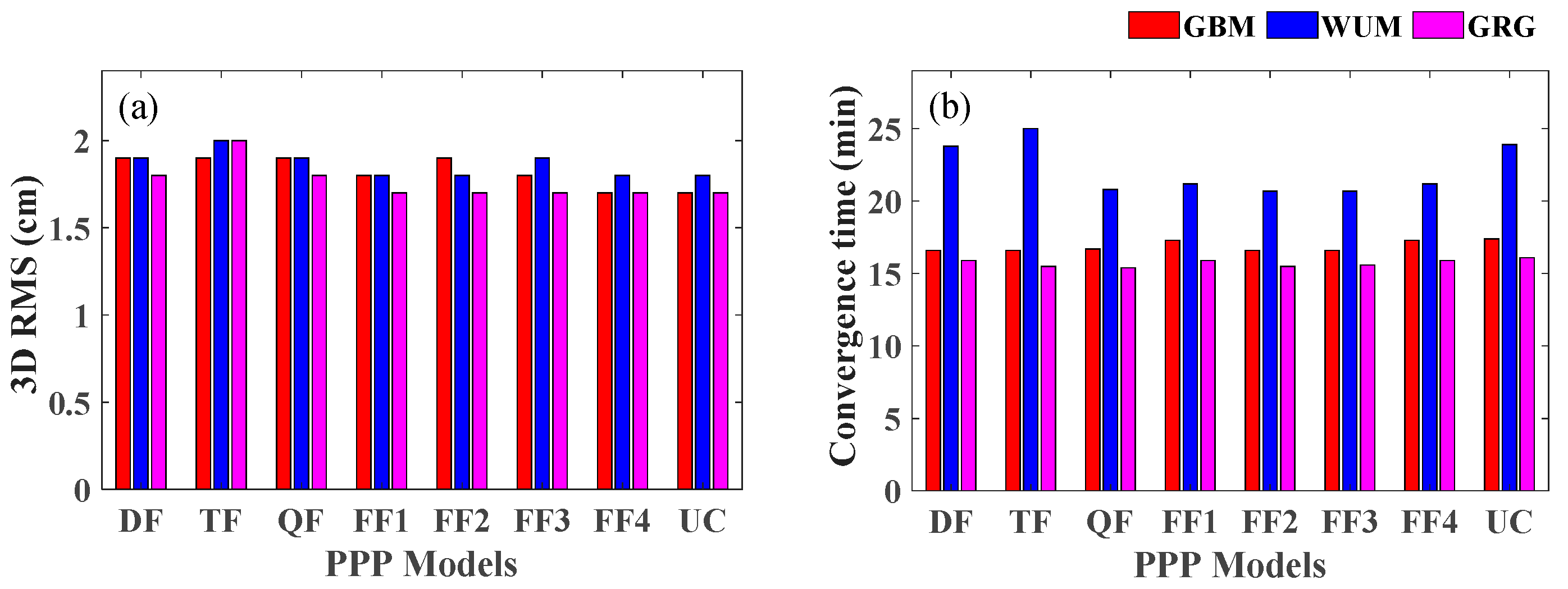
To further evaluate the performance of Galileo’s five-frequency PPP model, the WUM and GRG precise ephemeris and clock products are used for experiments. It should be noted that the GRG clock product has absorbed the UPD of the satellite side, and the GBM and WUM clock products have absorbed the UCD of the satellite side, with some differences. The average convergence times and average 3D RMS values at five stations of the DF, TF, QF, FF1, FF2, FF3, FF4 and UC PPP models are shown in
Figure 12.
The convergence times of the WUM product are significantly longer than those of the GBM and GRG products, and the average convergence time of the GRG product is the shortest. Compared with the dual-frequency PPP model, the multifrequency PPP model does not significantly improve the convergence speed. The average convergence times using the GBM, WUM and GRG products are 16.8 min, 22.2 min, and 15.7 min, respectively. Compared with the results using the GRM and WUM products, the average convergence speed obtained using the GRG product is increased by 6.8% and 29.1%, respectively. The average 3D RMS values obtained using the GBM, WUM and GRG products are 1.82 cm, 1.85 cm, and 1.77 cm, respectively. Compared with the results using the GRM and WUM products, the positioning accuracy achieved using the GRG product is improved by 2.7% and 4.3%, respectively.
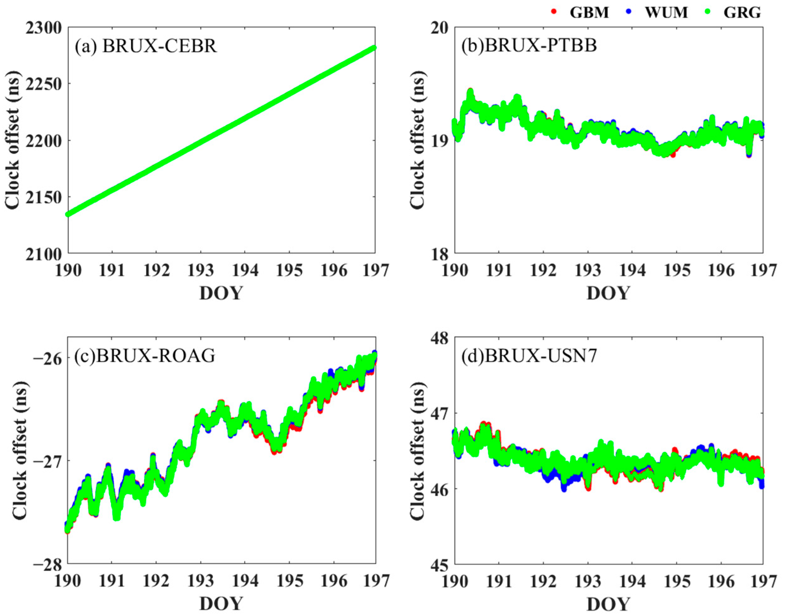
Limited by space,
Figure 13 only shows the clock offsets of the FF1 PPP model by using the GBM, WUM and GRG precise products. The clock offsets of the BRUX-CEBR, BRUX-PTBB and BRUX-ROAG time-frequency links are completely consistent, and there is only a small constant deviation term. Although the BRUX-USN7 clock offset trend is consistent, the deviation is slightly larger, which may be related to the quality of the observations of USN7. According to statistics, the deviations of the BRUX-CEBR link using GBM products compared with WUM and GRG products are 0.02 ns and 0.03 ns, respectively; the deviations of the BRUX-PTBB link using GBM products compared with WUM and GRG products are all 0.01 ns; the deviations of the BRUX-ROAG link using GBM products compared with WUM and GRG products are all 0.03 ns; and the deviations of the BRUX-USN7 link using GBM product compared with WUM and GRG products are 0.08 ns and 0.09 ns, respectively.
Table 6 shows the RMS values of the epoch difference by using WUM and GRG precision products for the PPP solution. The average RMS values of the BRUX-CEBR, BRUX-PTBB, BRUX-ROAG and BRUX-USN7 time-frequency links with the WUM product are 10.54 ps, 7.01 ps, 7.14 ps, and 8.24 ps, respectively, while those of the BRUX-CEBR, BRUX-PTBB, BRUX-ROAG and BRUX-USN7 time-frequency links with the GRG product are 10.57 ps, 7.02 ps, 7.22 ps, and 8.18 ps, respectively, which is consistent with the solution results obtained using the precise GBM product.
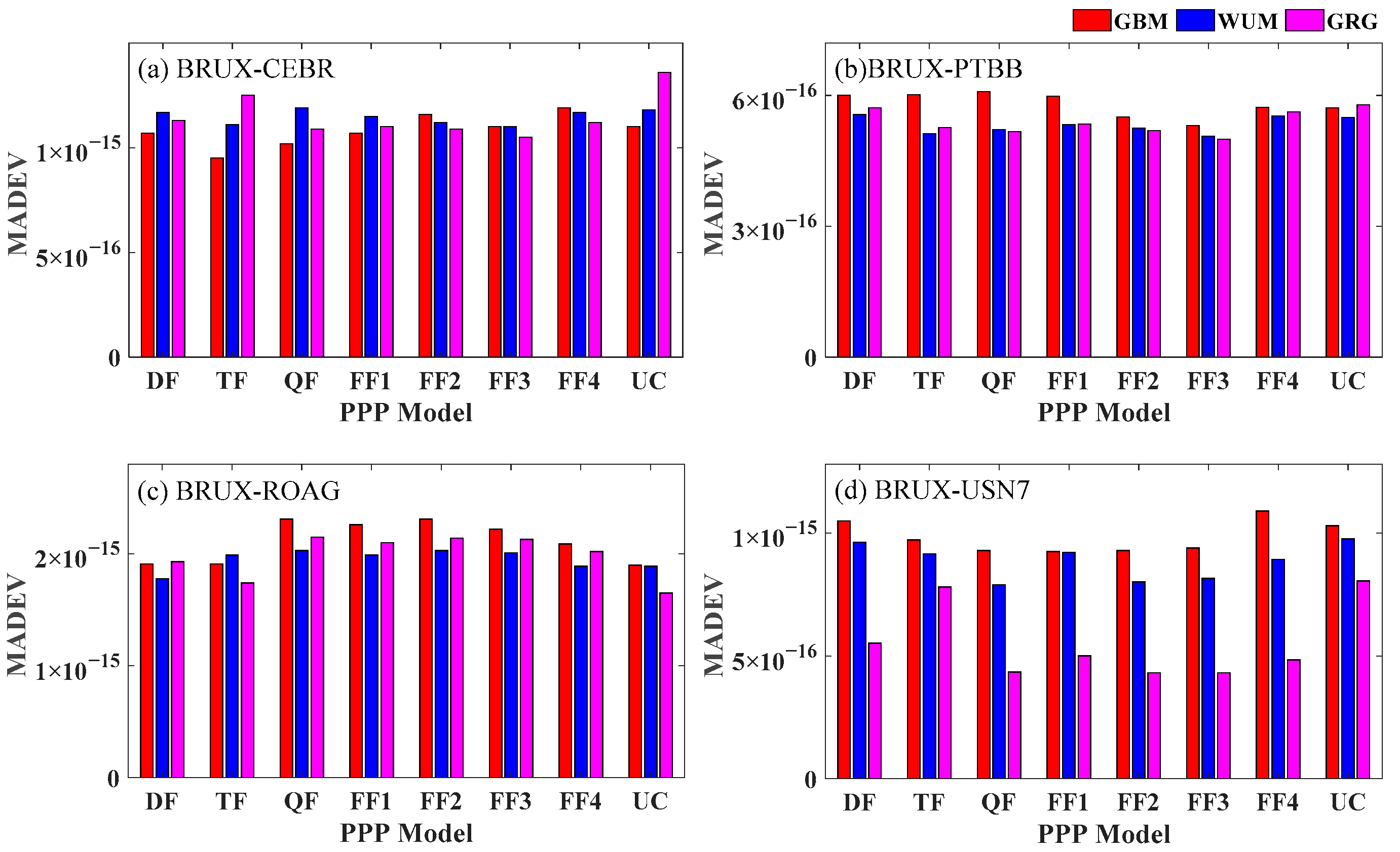
As shown in
Figure 14, the frequency stabilities of the BRUX-CEBR, BRUX-PTBB and BRUX-USN7 links can reach the 10
−16 level, and the frequency stability of the BRUX-USN7 link using the GRG product is the most significantly improved compared to those using WUM and GRG products, which may be related to the observation quality of USN7 and the absorption of satellite UPD by GRG clock products. The average frequency stabilities over four links using GBM, WUM and GRG products in 120,000 s are 1.18 × 10
−15, 1.13 × 10
−15 and 1.06 × 10
−15, respectively. Using WUM products, the average frequency stabilities of the DF, TF, QF, FF1, FF2, FF3, FF4 and UC PPP models are 1.12 × 10
−15, 1.13 × 10
−15, 1.13 × 10
−15, 1.15 × 10
−15, 1.12 × 10
−15, 1.11 × 10
−15, 1.13 × 10
−15, and 1.15 × 10
−15, respectively, while using GRG products, the corresponding average frequency stabilities are 1.05 × 10
−15, 1.07 × 10
−15, 1.05 × 10
−15, 1.06 × 10
−15, 1.05 × 10
−15, 1.03 × 10
−15, 1.05 × 10
−15 and 1.10 × 10
−15, respectively. All these results demonstrate that the frequency stability using the GRG product is better than those using WUM and GBM products at 120,000 s. It can also be found that compared with the DF model, the multifrequency model’s frequency stabilities are not significantly improved, which may be limited by the additional estimation of
IFB parameters and the accuracy of multifrequency
DCB products [
40].
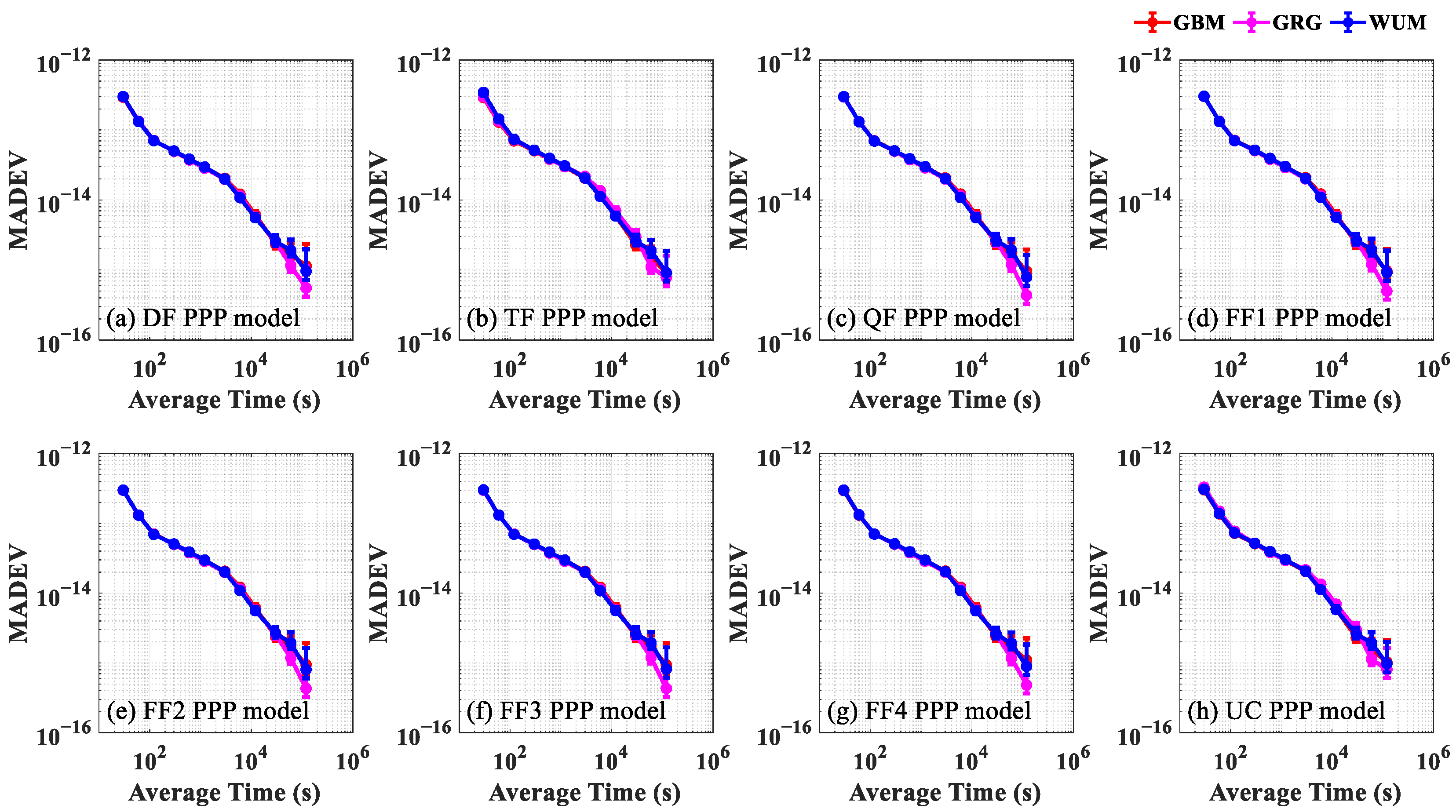
To deeply analyze the frequency transfer stability of the BRUX-USN7 link,
Figure 15 shows the frequency stability of the BRUX-USN7 link by using different ACs precision products. The frequency stability obtained using the GBM, WUM and GRG products before 30,000 s is completely consistent, but the frequency stability achieved using GRG products between 30,000 s and 120,000 s is significantly improved compared with using the GBM and WUM products. Compared with GBM and WUM, the stability obtained using GRG products is increased by 33.83% and 40.62% on average, respectively, and with the increase in time, the improvement range of stability gradually increases, which indicates that using GRG products has certain advantages over using GBM and WUM products in long-term frequency stability.
4. Discussion
With GNSS interoperability and support for multiple signal frequencies, the era of multi frequency and multi system PNT services has come. Compared with the traditional DF model, the multi frequency combination will be able to look for smaller noise coefficients, improve the reliability of the system, and help to achieve fast fixed ambiguity. At the same time, it will also face the challenge of IFB and IFCB processing in multi frequency signals. This research is a new exploration of Galileo five frequency signal PPP models, which systematically realizes the comparison and evaluation of Galileo TF, DT, FF, and DF models in terms of precision positioning and time-frequency transfer performance. Although the noise amplification factor of some multi frequency combination models decreases, the estimated IFB parameters are increased with the increase in the component observation equation. The precise separation of IFBs from clock bias and ambiguity parameters, the setting of multi frequency observation noise and the accuracy of multi frequency DCB products also affect the performance of five frequency PPP models. With the improvement of multi frequency DCB products, combined with the advantages of multi-frequency signals in redundancy, low noise, and long wavelength, it is reasonable to consider that Galileo five frequency signal will be more widely used in the future. In subsequent research, we will determine the noise of multi frequency observations and explore the performance of multi frequency signal in terms of ambiguity resolution.
It should be noted that in order to meet the performance of time-frequency transfer, we need to select the stations that support the Galileo five-frequency observation signals and are connected the external high-precision hydrogen atomic clocks. After eliminating stations with poor data quality and choosing the preferred stations of UTC laboratories, there are only a few proper suitable stations in the MGEX network. At the same time, scientists are more concerned about the index of the daily stability, which can basically reflect the best performance of the atomic clocks. The time-frequency links selected in this study are very representative, and the length of the observations can meet the requirements of short-term stability and long-term stability. In addition, our study evaluates the performance of positing and time-frequency transfer of double-, triple-, quad- and five-frequency PPP models, focusing on the comparison of results among different PPP models. Increasing the length of observations has no obvious practical significance and has little effect; the observations selected in our study can fully support our conclusions. The application of Galileo multi-frequency PPP solutions during different ionospheric active periods requires further investigation.
5. Conclusions
In this contribution, the mathematical PPP model of Galileo five-frequency observations is established; observation types, combination coefficients, ionospheric coefficients, and noise amplification coefficients from the DF to FF PPP models are also compared. Ranging from 464.6 km to 5991.2 km in four time-frequency links, there are seven-day observations from stations BRUX, CEBR, PTBB, ROAG and USN7 of the MGEX network. GBM, WUM and GRG precision orbits and clock products are used to evaluate the positioning performance and time-frequency transfer stability of the Galileo DF, TF, QF and FF PPP models.
Compared with the DF observation combination, although the multifrequency observation combination reduces noise and increases the redundancy and reliability of the observation equation, the positioning and time-frequency transfer performance are not significantly improved. The average 3D RMS values of the DF, TF, QF and FF1 PPP models are 1.88 cm, 1.95 cm, 1.85 cm, and 1.78 cm, respectively; and the average frequency stabilities of 120,000 s are 1.23 × 10⁻¹⁵, 1.15 × 10⁻¹⁵, 1.23 × 10⁻¹⁵, and 1.23 × 10⁻¹⁵, respectively. The differences in 3D RMS among the DF, TF, QF and FF1 PPP models are within 0.17 cm, and the differences in frequency stabilities are within 0.08 × 10⁻¹⁵. The performances of FF1, FF2, FF3, FF4 and UC PPP are also consistent with each other, the differences in 3D RMS values among the FF1, FF2, FF3, FF4 and UC PPP models are within 0.12 cm, and the differences in the frequency stabilities are within 0.02 × 10⁻¹⁵.
When using WUM and GRG precise products, the differences among the DF, TF, QF and FF PPP models in both positioning and time-frequency transfer performances are quite small, which is consistent with the results obtained using GBM products. The average convergence time obtained using the WUM product is the longest (22.2 min) and that which was achieved using the GRG product is the shortest (15.7 min). Using the GBM, WUM and GRG products, the average 3D RMS values are 1.82 cm, 1.85 cm, and 1.77 cm, respectively, and the average frequency stabilities at 120,000 s are better than 1.18 × 10⁻¹⁵, 1.13 × 10⁻¹⁵ and 1.06 × 10⁻¹⁵, respectively. These results show that the PPP performance using the GRG product is slightly better than that of GBM and WUM products, especially in terms of the long-term frequency stability of the BRUX-UNS7 link.
Author Contributions
Conceptualization, W.X. and W.-B.S.; methodology, W.X.; software, W.X.; validation, W.X., C.-H.C. and L.-H.L.; formal analysis, W.X., W.-B.S. and L.W.; investigation, W.X. and W.-B.S.; writing—original draft preparation, W.X.; writing-review and editing, W.X., W.-B.S., C.-H.C., L.-H.L., L.W. and Z.-Y.S.; visualization, W.X.; supervision, W.-B.S.; project administration, W.-B.S. All authors have read and agreed to the published version of the manuscript.
Funding
This work was funded by National Natural Science Foundations of China (Grant Nos. 41631072, 42030105, 41721003, 41804012, 41874023), Space Station Project (2020) (Grant No. 228), and the Natural Science Foundation of Hubei Province of China (Grant No. 2019CFB611).
Institutional Review Board Statement
Not applicable.
Informed Consent Statement
Not applicable.
Data Availability Statement
Acknowledgments
We gratefully acknowledge the IGS MGEX for providing Galileo observation data. We also acknowledge the WHU, GFZ and CNES for providing precise orbit and clock products.
Conflicts of Interest
The authors declare no conflict of interest.
References
- Hein, G.W. Status, perspectives and trends of satellite navigation. Satell. Navig. 2020, 1, 22. [Google Scholar] [CrossRef]
- Montenbruck, O.; Hugentobler, U.; Dach, R.; Steigenberger, P.; Hauschild, A. Apparent clock variations of the Block IIF-1 (SVN62) GPS satellite. GPS Solut. 2012, 16, 303–313. [Google Scholar] [CrossRef]
- Yang, Y.; Mao, Y.; Sun, B. Basic performance and future developments of BeiDou global navigation satellite system. Satell. Navig. 2020, 1, 1. [Google Scholar] [CrossRef] [Green Version]
- Zaminpardaz, S.; Teunissen, P.J.G.; Nadarajah, N. GLONASS CDMA L3 ambiguity resolution and positioning. GPS Solut. 2016, 21, 535–549. [Google Scholar] [CrossRef] [Green Version]
- Wang, K.; Chen, P.; Zaminpardaz, S.; Teunissen, P.J.G. Precise regional L5 positioning with IRNSS and QZSS: Stand-alone and combined. GPS Solut. 2018, 23, 10. [Google Scholar] [CrossRef] [Green Version]
- Diessongo, T.H.; Schüler, T.; Junker, S. Precise position determination using a Galileo E5 single-frequency receiver. GPS Solut. 2013, 18, 73–83. [Google Scholar] [CrossRef]
- Su, K.; Jin, S.; Jiao, G. Assessment of multi-frequency global navigation satellite system precise point positioning models using GPS, BeiDou, GLONASS, Galileo and QZSS. Meas. Sci. Technol. 2020, 31, 064008. [Google Scholar] [CrossRef]
- Chen, J.; Yue, D.; Zhu, S.; Liu, Z.; Zhao, X.; Xu, W. A new cycle slip detection and repair method for Galileo four-frequency observations. IEEE Access 2020, 8, 56528–56543. [Google Scholar] [CrossRef]
- Zhao, D.; Roberts, G.W.; Hancock, C.M.; Lau, L.; Bai, R. A triple-frequency cycle slip detection and correction method based on modified HMW combinations applied on GPS and BDS. GPS Solut. 2019, 23, 22. [Google Scholar] [CrossRef]
- Geng, J.; Bock, Y. Triple-frequency GPS precise point positioning with rapid ambiguity resolution. J. Geod. 2013, 87, 449–460. [Google Scholar] [CrossRef]
- Geng, J.; Guo, J. Beyond three frequencies: An extendable model for single-epoch decimeter-level point positioning by exploiting Galileo and BeiDou-3 signals. J. Geod. 2020, 94, 14. [Google Scholar] [CrossRef]
- Zhang, P.; Tu, R.; Gao, Y.; Liu, N.; Zhang, R. Improving Galileo’s carrier phase time transfer based on prior constraint information. J. Navig. 2018, 72, 121–139. [Google Scholar] [CrossRef]
- Petit, G. Sub-10−16 accuracy GNSS frequency transfer with IPPP. GPS Solut. 2021, 25, 22. [Google Scholar] [CrossRef]
- Leute, J.; Petit, G.; Exertier, P.; Samain, E.; Rovera, D.; Uhrich, P. High accuracy continuous time transfer with GPS IPPP and T2L2. In Proceedings of the 2018 European Frequency and Time Forum (EFTF), Turin, Italy, 10–12 April 2018; pp. 249–252. [Google Scholar]
- Tavella, P.; Petit, G. Precise time scales and navigation systems: Mutual benefits of timekeeping and positioning. Satell. Navig. 2020, 1, 10. [Google Scholar] [CrossRef]
- Dow, J.M.; Neilan, R.E.; Rizos, C. The International GNSS Service in a changing landscape of Global Navigation Satellite Systems. J. Geod. 2009, 83, 191–198. [Google Scholar] [CrossRef]
- Duong, V.; Harima, K.; Choy, S.; Laurichesse, D.; Rizos, C. Assessing the performance of multi-frequency GPS, Galileo and BeiDou PPP ambiguity resolution. J. Spat. Sci. 2019, 65, 61–78. [Google Scholar] [CrossRef]
- Tu, R.; Liu, J.; Zhang, R.; Zhang, P.; Huang, X.; Lu, X. RTK model and positioning performance analysis using Galileo four-frequency observations. Adv. Space Res. 2019, 63, 913–926. [Google Scholar] [CrossRef]
- Liu, X.; Jiang, W.; Chen, H.; Zhao, W.; Huo, L.; Huang, L.; Chen, Q. An analysis of inter-system biases in BDS/GPS precise point positioning. GPS Solut. 2019, 23, 116. [Google Scholar] [CrossRef]
- Qin, W.; Ge, Y.; Wei, P.; Dai, P.; Yang, X. Assessment of the BDS-3 on-board clocks and their impact on the PPP time transfer performance. Measurement 2020, 153, 107356. [Google Scholar] [CrossRef]
- Li, X.; Liu, G.; Li, X.; Zhou, F.; Feng, G.; Yuan, Y.; Zhang, K. Galileo PPP rapid ambiguity resolution with five-frequency observations. GPS Solut. 2019, 24, 24. [Google Scholar] [CrossRef]
- Zhang, P.; Tu, R.; Gao, Y.; Zhang, R.; Han, J. Performance of Galileo precise time and frequency transfer models using quad-frequency carrier phase observations. GPS Solut. 2020, 24, 40. [Google Scholar] [CrossRef]
- Liu, T.; Jiang, W.; Laurichesse, D.; Chen, H.; Liu, X.; Wang, J. Assessing GPS/Galileo real-time precise point positioning with ambiguity resolution based on phase biases from CNES. Adv. Space Res. 2020, 66, 810–825. [Google Scholar] [CrossRef]
- Kuang, K.; Li, J.; Zhang, S. Galileo real-time orbit determination with multi-frequency raw observations. Adv. Space Res. 2021, 67, 3147–3155. [Google Scholar] [CrossRef]
- Su, K.; Jin, S. Analytical performance and validations of the Galileo five-frequency precise point positioning models. Measurement 2021, 172, 108890. [Google Scholar] [CrossRef]
- Jin, S.; Su, K. PPP models and performances from single- to quad-frequency BDS observations. Satell. Navig. 2020, 1, 16. [Google Scholar] [CrossRef]
- Ge, Y.; Cao, X.; Shen, F.; Yang, X.; Wang, S. BDS-3/Galileo time and frequency transfer with quad-frequency precise point positioning. Remote Sens. 2021, 13, 2704. [Google Scholar] [CrossRef]
- Leick, A.; Rapoport, L.; Tatarnikov, D. GPS Satellite Surveying, 4th ed.; John Wiley & Sons: New York, NY, USA, 2015; pp. 1–807. [Google Scholar]
- Liu, T.; Chen, H.; Chen, Q.; Jiang, W.; Laurichesse, D.; An, X.; Geng, T. Characteristics of phase bias from CNES and its application in multi-frequency and multi-GNSS precise point positioning with ambiguity resolution. GPS Solut. 2021, 25, 58. [Google Scholar] [CrossRef]
- Li, X.; Li, X.; Liu, G.; Feng, G.; Yuan, Y.; Zhang, K.; Ren, X. Triple-frequency PPP ambiguity resolution with multi-constellation GNSS: BDS and Galileo. J. Geod. 2019, 93, 1105–1122. [Google Scholar] [CrossRef]
- Zhao, L.; Ye, S.; Song, J. Handling the satellite inter-frequency biases in triple-frequency observations. Adv. Space Res. 2017, 59, 2048–2057. [Google Scholar] [CrossRef]
- Zhang, B.; Teunissen, P.J.; Yuan, Y.; Zhang, H.; Li, M. Joint estimation of vertical total electron content (VTEC) and satellite differential code biases (SDCBs) using low-cost receivers. J. Geod. 2018, 92, 401–413. [Google Scholar] [CrossRef] [Green Version]
- Petit, G.; Luzum, B. IERS Conventions (2010); IERS Technical Note No. 36; Bureau International des Poids et Mesures Sevres: Frankfurt am Main, Germany, 2010. [Google Scholar]
- Kouba, J. A Guide to Using International GNSS Service (IGS) Products; Jet Propulsion Laboratory: Pasadena, CA, USA, 2009; p. 34.
- Wu, J.-T.; Wu, S.C.; Hajj, G.A.; Bertiger, W.I.; Lichten, S.M. Effects of antenna orientation on GPS carrier phase. In Proceedings of the Astrodynamics 1991, San Diego, CA, USA, 19–22 August 1991; pp. 1647–1660. [Google Scholar]
- Lyard, F.; Lefevre, F.; Letellier, T.; Francis, O. Modelling the global ocean tides: Modern insights from FES2004. Ocean Dyn. 2006, 56, 394–415. [Google Scholar] [CrossRef]
- Saastamoinen, J. Contributions to the theory of atmospheric refraction. Bull. Géodésique (1946–1975) 1973, 107, 13–34. [Google Scholar] [CrossRef]
- Böhm, J.; Heinkelmann, R.; Schuh, H. Short note: A global model of pressure and temperature for geodetic applications. J. Geod. 2007, 81, 679–683. [Google Scholar] [CrossRef]
- Böhm, J.; Niell, A.; Tregoning, P.; Schuh, H. Global Mapping Function (GMF): A new empirical mapping function based on numerical weather model data. Geophys. Res. Lett. 2006, 33, 3–6. [Google Scholar] [CrossRef] [Green Version]
- Ge, Y.; Ding, S.; Qin, W.; Zhou, F.; Wang, S. Performance of ionospheric-free PPP time transfer models with BDS-3 quad-frequency observations. Measurement 2020, 160, 107836. [Google Scholar] [CrossRef]
Figure 1.
Geographic distribution of the selected stations.
Figure 1.
Geographic distribution of the selected stations.
Figure 2.
Distribution of number of visible satellites and position dilution of precision (PDOP) value for GPS and Galileo constellation on days of year (DOYs) 190 to 196 in 2020. (a) Number of visible GPS satellites; (b) GPS PDOP values; (c) number of visible Galileo satellites; and (d) Galileo PDOP values.
Figure 3.
Number of visible satellites and time dilution of precision (TDOP) values at BRUX and PTBB for Galileo on DOYs 190 to 196 in 2020. (a) Number of visible satellites; and (b) TDOP values.
Figure 3.
Number of visible satellites and time dilution of precision (TDOP) values at BRUX and PTBB for Galileo on DOYs 190 to 196 in 2020. (a) Number of visible satellites; and (b) TDOP values.
Figure 4.
Galileo multipath combination noise sequence and elevation at frequencies E1, E5a, E6, E5 and E5b at BRUX station on DOYs 190 to 196 in 2020. (a) E08 satellite; (b) E15 satellite; (c) E25 satellite; and (d) E33 satellite.
Figure 4.
Galileo multipath combination noise sequence and elevation at frequencies E1, E5a, E6, E5 and E5b at BRUX station on DOYs 190 to 196 in 2020. (a) E08 satellite; (b) E15 satellite; (c) E25 satellite; and (d) E33 satellite.
Figure 5.
Positioning performance of BRUX, CEBR, PTBB, ROAG and USN7 stations for the DF, TF, QF and FF1 PPP models on DOYs 190 to 196 in 2020. (a) E component RMS value; (b) N component RMS value; (c) U component RMS value; and (d) convergence time.
Figure 5.
Positioning performance of BRUX, CEBR, PTBB, ROAG and USN7 stations for the DF, TF, QF and FF1 PPP models on DOYs 190 to 196 in 2020. (a) E component RMS value; (b) N component RMS value; (c) U component RMS value; and (d) convergence time.
Figure 6.
Clock offset sequence at four time-frequency links for the DF, TF, QF and FF1 PPP models on DOYs 190 to 196 in 2020. (a) BRUX-CEBR time-frequency link; (b) BRUX-PTBB time-frequency link; (c) BRUX-ROAG time-frequency link; and (d) BRUX-USN7 time-frequency link.
Figure 6.
Clock offset sequence at four time-frequency links for the DF, TF, QF and FF1 PPP models on DOYs 190 to 196 in 2020. (a) BRUX-CEBR time-frequency link; (b) BRUX-PTBB time-frequency link; (c) BRUX-ROAG time-frequency link; and (d) BRUX-USN7 time-frequency link.
Figure 7.
MADEV at four time-frequency links for the DF, TF, QF and FF1 PPP solutions on DOYs 190 to 196 in 2020. (a) BRUX-CEBR time-frequency link; (b) BRUX-PTBB time-frequency link; (c) BRUX-ROAG time-frequency link; and (d) BRUX-USN7 time-frequency link.
Figure 7.
MADEV at four time-frequency links for the DF, TF, QF and FF1 PPP solutions on DOYs 190 to 196 in 2020. (a) BRUX-CEBR time-frequency link; (b) BRUX-PTBB time-frequency link; (c) BRUX-ROAG time-frequency link; and (d) BRUX-USN7 time-frequency link.
Figure 8.
Positioning performance of the BRUX, CEBR, PTBB, ROAG and USN7 stations by the FF1, FF2, FF3, FF4 and UC PPP solutions on DOYs 190 to 196 in 2020. (a) E Component RMS value; (b) N component RMS value; (c) U component RMS value; and (d) convergence time.
Figure 8.
Positioning performance of the BRUX, CEBR, PTBB, ROAG and USN7 stations by the FF1, FF2, FF3, FF4 and UC PPP solutions on DOYs 190 to 196 in 2020. (a) E Component RMS value; (b) N component RMS value; (c) U component RMS value; and (d) convergence time.
Figure 9.
Clock offset sequences at four time-frequency links for the FF1, FF2, FF3, FF4 and UC PPP solutions on DOYs 190 to 196 in 2020. (a) BRUX-CEBR time-frequency link; (b) BRUX-PTBB time-frequency link; (c) BRUX-ROAG time-frequency link; and (d) BRUX-USN7 time-frequency link.
Figure 9.
Clock offset sequences at four time-frequency links for the FF1, FF2, FF3, FF4 and UC PPP solutions on DOYs 190 to 196 in 2020. (a) BRUX-CEBR time-frequency link; (b) BRUX-PTBB time-frequency link; (c) BRUX-ROAG time-frequency link; and (d) BRUX-USN7 time-frequency link.
Figure 10.
MADEV at four time-frequency links for the FF1, FF2, FF3, FF4 and UC PPP solutions on DOYs 190 to 196 in 2020. (a) BRUX-CEBR time-frequency link; (b) BRUX-PTBB time-frequency link; (c) BRUX-ROAG time-frequency link; and (d) BRUX-USN7 time-frequency link.
Figure 10.
MADEV at four time-frequency links for the FF1, FF2, FF3, FF4 and UC PPP solutions on DOYs 190 to 196 in 2020. (a) BRUX-CEBR time-frequency link; (b) BRUX-PTBB time-frequency link; (c) BRUX-ROAG time-frequency link; and (d) BRUX-USN7 time-frequency link.
Figure 11.
IFB sequences at five stations for the FF2, FF3, FF4 and UC PPP models on DOYs 190 to 196 in 2020. (a) BRUX station; (b) CEBR station; (c) PTBB station; (d) ROAG station; and (e) USN7 station.
Figure 11.
IFB sequences at five stations for the FF2, FF3, FF4 and UC PPP models on DOYs 190 to 196 in 2020. (a) BRUX station; (b) CEBR station; (c) PTBB station; (d) ROAG station; and (e) USN7 station.
Figure 12.
Average 3D RMS values and average convergence times by using the GBM, WUM and GRG precise product PPP solutions on DOYs 190 to 196 in 2020. (a) 3D RMS value; (b) convergence time.
Figure 12.
Average 3D RMS values and average convergence times by using the GBM, WUM and GRG precise product PPP solutions on DOYs 190 to 196 in 2020. (a) 3D RMS value; (b) convergence time.
Figure 13.
Clock offset sequences of the GBM, WUM and GRG products in the PPP FF1 model. (a) BRUX-CEBR time-frequency link; (b) BRUX-PTBB time-frequency link; (c) BRUX-ROAG time-frequency link; and (d) BRUX-USN7 time-frequency link.
Figure 13.
Clock offset sequences of the GBM, WUM and GRG products in the PPP FF1 model. (a) BRUX-CEBR time-frequency link; (b) BRUX-PTBB time-frequency link; (c) BRUX-ROAG time-frequency link; and (d) BRUX-USN7 time-frequency link.
Figure 14.
MADEV of the PPP solution by using GBM, WUM and GRG precision products at 120,000 s. (a) BRUX-CEBR time-frequency link; (b) BRUX-PTBB time-frequency link; (c) BRUX-ROAG time-frequency link; and (d) BRUX-USN7 time-frequency link.
Figure 14.
MADEV of the PPP solution by using GBM, WUM and GRG precision products at 120,000 s. (a) BRUX-CEBR time-frequency link; (b) BRUX-PTBB time-frequency link; (c) BRUX-ROAG time-frequency link; and (d) BRUX-USN7 time-frequency link.
Figure 15.
MADEV at the BRUX-USN7 time-frequency link of the PPP solution by using GBM, WUM and GRG precision products on DOYs 190 to 196 in 2020. (a) DF PPP model; (b) TF PPP model; (c) QF PPP model; (d) FF1 PPP model; and (e) FF2 PPP model; (f) FF3 PPP model; (g) FF4 PPP model; (h) UC PPP model.
Figure 15.
MADEV at the BRUX-USN7 time-frequency link of the PPP solution by using GBM, WUM and GRG precision products on DOYs 190 to 196 in 2020. (a) DF PPP model; (b) TF PPP model; (c) QF PPP model; (d) FF1 PPP model; and (e) FF2 PPP model; (f) FF3 PPP model; (g) FF4 PPP model; (h) UC PPP model.
Table 1.
Summarization of Galileo DF, TF, QF and FF PPP models.
Table 1.
Summarization of Galileo DF, TF, QF and FF PPP models.
| Models | Observed Type | E1 | E5a | E5b | E5 | E6 | Ion | Noise |
|---|
| DF | E1/E5a | 2.261 | −1.261 | / | / | / | / | 2.588 |
| TF | E1/E5a/E5b | 2.315 | −0.836 | −0.479 | / | / | / | 2.507 |
| QF | E1/E5a/E5b/E5 | 2.317 | −0.606 | −0.274 | −0.437 | / | / | 2.450 |
| FF1 | E1/E5a/E5b/E5/E6 | 2.217 | −0.680 | −0.351 | −0.512 | 0.326 | / | 2.423 |
| FF2 | E1/E5a/E5b/E5 | 2.317 | −0.606 | −0.274 | −0.437 | / | / | 2.450 |
| E1/E5a/E5b/E6 | 2.255 | −0.904 | −0.545 | 0.193 | / | / | 2.497 |
| FF3 | E1/E5a/E5b | 2.315 | −0.836 | −0.479 | / | / | / | 2.507 |
| E1/E5a/E5 | 2.293 | 0.734 | −0.559 | / | / | / | 2.471 |
| E1/E5a/E6 | 2.269 | −1.244 | −0.024 | / | / | / | 2.588 |
| FF4 | E1/E5a | 2.261 | −1.261 | / | / | / | / | 2.588 |
| E1/E5b | 2.422 | / | −1.422 | / | / | / | 2.809 |
| E1/E5 | 2.338 | / | / | −1.338 | / | / | 2.694 |
| E1/E6 | 2.931 | / | / | / | −1.931 | / | 3.510 |
| UC | E1 | 1.000 | / | / | / | / | 1.000 | 1.000 |
| E5a | / | 1.000 | / | / | / | 1.793 | 1.000 |
| E5b | / | / | 1.000 | / | / | 1.703 | 1.000 |
| E5 | / | / | / | 1.000 | / | 1.747 | 1.000 |
| E6 | / | / | / | / | 1.000 | 1.518 | 1.000 |
Table 2.
List of selected MGEX stations.
Table 2.
List of selected MGEX stations.
| Stations | Receiver | Antenna | Clock | Country | Distance |
|---|
| BRUX | SEPT POLARX5TR | JAVRINGANT_DM | UTC (ORB) | Belgium | / |
| CEBR | SEPT POLARX5TR | SEPCHOKE_B3E6 | H-MASER | Spain | 1331.6 km |
| PTBB | SEPT POLARX5TR | LEIAR25.R4 | UTC (PTB) | Germany | 454.6 km |
| ROAG | SEPT POLARX5TR | LEIAR25.R4 | UTC (ROA) | Spain | 1796.3 km |
| USN7 | SEPT POLARX5TR | TPSCR.G5 | UTC (USNO) | America | 5991.2 km |
Table 3.
Detailed processing strategies.
Table 3.
Detailed processing strategies.
| Items | Strategies |
|---|
| Solutions | DF/TF/QF/FF1/FF2/FF2/FF3/FF4/UC PPP models |
| Observations | E1/E5a/E5b/E5/E6 observations |
| Elevation cutoff | 7° |
| Orbits and clock | GBM, WUM and GRG precise products |
| Satellite DCB | CAS BSX products [32],
E5b:, E5:,
E6: |
| Earth rotation | Corrected [33] |
| Relativistic effect | Corrected [34] |
| Phase windup effect | Corrected [35] |
| Tide effect | Corrected [36] |
| PCO/PCV | IGS14.atx |
| Station coordinates | Estimated as constants |
| Receiver clock | Estimated as white noises (104 m2/s) |
| Ionospheric delay | UC: Estimated as random walk process
DF/TF/QF/FF1/FF2/FF3/FF4: Eliminated
first-order by IF combinations |
| Tropospheric delay | Dry component: GPT add Saastamoinen model [37,38]
Wet component: Estimated as random walk part (10−8 m2/s), GMF mapping function [39] |
| Ambiguities | Estimated as constant, float solution |
Table 4.
Clock offset epoch difference results of average (AVG) and root mean square (RMS) at four time-frequency links for the DF, TF, QF and FF1 PPP models on DOYs 190 to 196 in 2020 (ps).
Table 4.
Clock offset epoch difference results of average (AVG) and root mean square (RMS) at four time-frequency links for the DF, TF, QF and FF1 PPP models on DOYs 190 to 196 in 2020 (ps).
| Items | Links | DF | TF | QF | FF1 |
|---|
| AVG | BRUX-CEBR | 7.38 | 7.38 | 7.38 | 7.38 |
| BRUX-PTBB | 0.01 | 0.01 | 0.01 | 0.01 |
| BRUX-ROAG | 0.08 | 0.08 | 0.08 | 0.08 |
| BRUX-USN7 | −0.01 | −0.01 | −0.01 | −0.01 |
| RMS | BRUX-CEBR | 10.54 | 10.44 | 10.50 | 10.49 |
| BRUX-PTBB | 7.02 | 6.88 | 6.97 | 6.87 |
| BRUX-ROAG | 7.22 | 7.09 | 7.17 | 7.14 |
| BRUX-USN7 | 7.98 | 7.88 | 8.02 | 8.14 |
Table 5.
Clock offset epoch difference results at four time-frequency links for the FF1, FF2, FF3, FF4 and UC PPP models on DOYs 190 to 196 in 2020 (ps).
Table 5.
Clock offset epoch difference results at four time-frequency links for the FF1, FF2, FF3, FF4 and UC PPP models on DOYs 190 to 196 in 2020 (ps).
| Item | Links | FF1 | FF2 | FF3 | FF4 | UC |
|---|
| AVG | BRUX-CEBR | 7.38 | 7.38 | 7.40 | 7.38 | 7.38 |
| BRUX-PTBB | 0.01 | 0.01 | 0.01 | −0.01 | 0.01 |
| BRUX-ROAG | 0.08 | 0.08 | 0.08 | 0.08 | 0.08 |
| BRUX-USN7 | −0.01 | −0.01 | −0.01 | −0.01 | −0.01 |
| RMS | BRUX-CEBR | 10.49 | 10.51 | 10.53 | 10.40 | 10.46 |
| BRUX-PTBB | 6.87 | 6.92 | 6.95 | 6.84 | 6.92 |
| BRUX-ROAG | 7.14 | 7.15 | 7.16 | 7.09 | 7.03 |
| BRUX-USN7 | 8.14 | 8.04 | 8.04 | 8.00 | 8.23 |
Table 6.
Clock offset epoch difference RMS at four time-frequency links by the WUM and GRG product PPP solutions on DOYs 190 to 196 in 2020 (ps).
Table 6.
Clock offset epoch difference RMS at four time-frequency links by the WUM and GRG product PPP solutions on DOYs 190 to 196 in 2020 (ps).
| Products | Links | DF | TF | QF | FF1 | FF2 | FF3 | FF4 | UC |
|---|
| WUM | BRUX-CEBR | 10.62 | 10.59 | 10.55 | 10.49 | 10.49 | 10.52 | 10.52 | 10.55 |
| BRUX-PTBB | 7.1 | 7.02 | 7.04 | 6.96 | 7.02 | 7.02 | 6.95 | 6.98 |
| BRUX-ROAG | 7.27 | 7.11 | 7.16 | 7.12 | 7.16 | 7.16 | 7.04 | 7.13 |
| BRUX-USN7 | 8.08 | 9.02 | 8.05 | 8.15 | 8.11 | 8.08 | 8.34 | 8.06 |
| GRG | BRUX-CEBR | 10.65 | 10.53 | 10.54 | 10.51 | 10.55 | 10.51 | 10.76 | 10.52 |
| BRUX-PTBB | 7.08 | 7.01 | 7.00 | 6.92 | 6.99 | 6.91 | 7.31 | 6.96 |
| BRUX-ROAG | 7.30 | 7.24 | 7.21 | 7.17 | 7.20 | 7.16 | 7.27 | 7.19 |
| BRUX-USN7 | 8.07 | 8.11 | 8.00 | 8.12 | 8.04 | 8.11 | 8.92 | 8.03 |
| Publisher’s Note: MDPI stays neutral with regard to jurisdictional claims in published maps and institutional affiliations. |
© 2021 by the authors. Licensee MDPI, Basel, Switzerland. This article is an open access article distributed under the terms and conditions of the Creative Commons Attribution (CC BY) license (https://creativecommons.org/licenses/by/4.0/).


 ,
, 


