Nonstationary Extreme Value Analysis of Nearshore Sea-State Parameters under the Effects of Climate Change: Application to the Greek Coastal Zone and Port Structures

Abstract

In the present work, a methodological framework, based on nonstationary extreme value analysis of nearshore sea-state parameters, is proposed for the identification of climate change impacts on coastal zone and port defense structures. The applications refer to the estimation of coastal hazards on characteristic Mediterranean microtidal littoral zones and the calculation of failure probabilities of typical rubble mound breakwaters in Greek ports. The proposed methodology hinges on the extraction of extreme wave characteristics and sea levels due to storm events affecting the coast, a nonstationary extreme value analysis of sea-state parameters and coastal responses using moving time windows, a fitting of parametric trends to nonstationary parameter estimates of the extreme value models, and an assessment of nonstationary failure probabilities on engineered port protection. The analysis includes estimation of extreme total water level (TWL) on several Greek coasts to approximate the projected coastal flooding hazard under climate change conditions in the 21st century. The TWL calculation considers the wave characteristics, sea level height due to storm surges, mean sea level (MSL) rise, and astronomical tidal ranges of the study areas. Moreover, the failure probabilities of a typical coastal defense structure are assessed for several failure mechanisms, considering variations in MSL, extreme wave climates, and storm surges in the vicinity of ports, within the framework of reliability analysis based on the nonstationary generalized extreme value (GEV) distribution. The methodology supports the investigation of future safety levels and possible periods of increased vulnerability of the studied structure to different ultimate limit states under extreme marine weather conditions associated with climate change, aiming at the development of appropriate upgrading solutions. The analysis suggests that the assumption of stationarity might underestimate the total failure probability of coastal structures under future extreme marine conditions.

1. Introduction

Global climate change is expected to cause significant long-term changes in storm variability regionally, leading to consequent shifts in mean sea level (MSL), wave climate and storm surge regimes [1,2,3]. The general inception of a changing climate with extreme marine weather events of higher intensity and frequency in tandem with MSL rise increases the vulnerability and exposure of coastal areas to inundation, flooding, and erosion hazards, as well as of port and harbor protection structures to different failure mechanisms, ultimately resulting in an inability to fulfill their requirements. The projected increase of future hydraulic loading conditions, combined with the limited residual service lifetime of many of the existing coastal defenses, creates an urgent need for a reliable estimation of future extreme sea conditions in nearshore areas, as well as of failure probabilities for port structures and harbor defenses under such extremes. This is a very important issue for integrated coastal zone management in the 21st century, as coastal areas worldwide are densely populated and assemble many significant economic activities.

1.1. Literature Review

Climate change impacts on coastal zones are generally associated with rising MSL, but also with significant changes in the frequency and intensity of extreme marine storm events [1,2,3]. In the Mediterranean region, even if the majority of scientific studies have focused on the variability and long-term trends of MSL [4,5,6,7,8], shifts in extreme storm surges and waves under climate change have also been systematically examined during the last decade. Climate change effects on extreme wave storm events (specifically in the Mediterranean) have been examined, among others, by Méndez et al. [9], Lionello et al. [10], Benetazzo et al. [11], Casas-Prat and Sierra [12], Galiatsatou and Prinos [13,14] and Makris et al. [15]. Even if climate change impact studies on the extreme marine climate of the Mediterranean have gained increasing interest, scientific studies to assess the vulnerability of coastal areas to flooding and erosion hazards under changing climatic conditions are still relatively limited [16,17,18,19,20,21,22,23].

The estimation of extreme total water level (TWL) at a coastal area involves assessing the contributions of various components of the marine climate, namely based on the sum of wave-induced run-up on the coastline, the storm surge level, the MSL rise, and the high tides. Thus, TWL can provide the boundary conditions for flooding and erosion hazard studies and the estimation of related coastal risks. Very recently, studies focusing on estimating TWL at the shoreline have started including components to simulate seasonality, interannual variability, and trends of the marine climate, as well as considering dependencies between the different variables of TWL [24,25,26].

The effects of climate change on engineered waterfronts (i.e., coastal protection works and port structures at harbored areas) has received considerable attention only during the last decade [27,28,29,30,31,32]. Becker et al. [27], Suh et al. [28], Sekimoto et al. [29], Isobe [30], and Sánchez-Arcilla et al. [31] studied the possible effects of climate change on coastal defenses and on port and harbor operations. Burcharth et al. [32] presented several methods to upgrade typical embankments under climate change conditions. In more locally focused applications, e.g., Koftis et al. [33] and Karambas et al. [34] studied the vulnerability of coastal and harbor structures in Greece due to climate change impacts and proposed indicative upgrading methods.

The overall framework of integrated risk management includes the analysis and assessment of risks and implementation of risk reduction/mitigation options [35]. Risk-based approaches are currently gaining ground in the process of evaluating safety of coastal structures subject to increased exposure due to extreme marine conditions. Reliability analysis, corresponding to assessing failure probabilities of such engineered defenses, forms an inherent part of a risk-based approach to designing new or evaluating the performance of existing coastal structures. Castillo et al. [36], Dai Viet et al. [37], Van Gelder et al. [38], Buijs et al. [39], Kim & Suh [40], Galiatsatou and Prinos [41], Naulin et al. [42], Nepal et al. [43] and Galiatsatou et al. [44] performed reliability analysis of coastal and harbor structures to determine failure probabilities including different failure mechanisms of the defenses, and further proposed modern (both probabilistic and stochastic) methods and techniques to be included either in the engineering design phase or the construction upgrading process.

Quite recently, the risk of global port operations due to climate change was investigated around the world within a probabilistic evaluation approach [45]. Moreover, the probabilistic assessment of port operation downtime was also reviewed under the effects of climate change, based on a hybrid statistic-dynamical framework combining a weather generator and a metamodel [46]. Focusing on the Mediterranean Sea, a review of potential physical impacts on harbors under climate change was presented analyzing port operations and infrastructure performance considering relative sea level, wave storm features (height, period, direction, and duration) and combined effects as key climatic factors [47]. Seaport climate change impact assessment was also recently presented [48] with use of a multi-level methodology following a sequential path that starts with a quantitative analysis focused on multi-hazard and multi-impact evaluation with climate information based on indicators. More localized in-depth analyses of important case studies refer to addressing long-term operational risk management in port docks under climate change, modelling the impact of climate change on Spanish harbors’ operability, and reliability-based investigations of breakwater structures including the economic impact on port activities [49,50,51]. Malliouri et al. [52,53] have also performed a reliability analysis of rubble mound breakwaters based on an easy-to-use methodology to assess the failure probabilities of coastal structures based on probabilistic representation of sea conditions at the structures’ location. Radfar et al. [54] compared a commonly applied and joint probability approach for the design of a conventional rubble mound breakwater at the Makran coasts on the southern coast of Iran. The effects of climate change on the overtopping failure mechanism of the breakwater were also discussed, indicating that a higher freeboard and a lower overtopping discharge in the new design approach can reduce the vulnerability of the structure against projected future environmental changes.

Several European and international standards for the design and construction of breakwaters (and port structures in general) comprise certain manuals, recommendations and guidelines reports, such as the Puerto del Estado’s ROM 1.1 and PIANC’s Report 196–2016 [55,56]. These refer to all-inclusive manuals that concentrate information and application guidelines for breakwater design with certain aspects of the reliability concept, mostly aiming at completing the regulatory framework for maritime infrastructure design. In the latter, the evaluation of reliability is mainly performed based on simplified standard statistics, assisted by diagrams of components within synthetic cycles, and then followed by spreading activation networks, designing of decision trees, validated by physical model tests. Especially, in [55] a detailed roadmap of breakwater reliability estimation procedures is provided based on applied statistics for coastal and port structures’ risk management.

1.2. Scope of Research

Natural climatic variability, human interventions in the hydrologic cycle, and anthropogenic climate change are some of the prominent causes of nonstationarities inherent to marine signals. Long-term nonstationarities in the marine climate variables, mainly attributed to climate change, necessitate the use of nonstationary approaches to assess: (a) reliable future extremes of TWL on the coast to be used as input for various impact studies, and (b) robust future failure probabilities of existing coastal and harbor structures for different failure mechanisms, allowing one to determine their future safety levels as well as to develop appropriate upgrading solutions where needed.

However, the majority of existing studies in the abovementioned fields assume stationarity of the marine climate variables and/or do not consider their combined impact on coastal areas and coastal or harbor structures. In the present work, climate change impacts on nearshore sea-state parameters are assessed within a nonstationary probabilistic framework developed for estimating coastal hazards, as well as failure probabilities of coastal defenses. The former includes an estimation of extreme TWLs on different coasts of Greece by the use of a nonstationary approach to approximate the coastal flooding hazard under climate change conditions. Wave characteristics, sea level height (SLH) due to storm surges, MSL rise, and astronomical tidal range of the study areas are considered in the analysis. The latter investigates the performance of a selected conventional rubble mound breakwater to different failure mechanisms under extreme marine conditions associated with climate change. Failure probabilities of the breakwater structure are assessed for different failure mechanisms, considering variations in MSL, extreme wave climate and storm surge, within the general framework of nonstationary reliability analysis. The methodological approach followed in the two applications included in this study is presented in Figure 1.

2. Modeling Methods and Available Datasets for the Study Region and Focus Areas

The modeling methodology of the present work refers to dynamically downscaled simulations of marine characteristics in long-term climatic mode (50-year spans for 150 years; 1951–2100) at the east-central part of the Mediterranean Sea [15,57,58]. Based on these, the proposed extreme value analysis (EVA) techniques (see Section 3) have been implemented to the extremes of SLH and the associated random wave characteristics (H_so and corresponding T_p) in offshore waters of selected areas in the Aegean Sea. Nearshore wave-induced sea levels (η_w and R_2%) have been estimated well as with a special focus on the coastal zones of the northern, middle, and southern Aegean basin [13,14,15,23,26]. These refer to the first application presented herein, focusing on three representative study areas with a reported high risk of coastal flooding [13,14,15,23,59]. The second application comprises a detailed failure probability analysis of a coastal structure located at a selected port in northern Greece dealing with technical issues of port operation during extreme marine weather conditions.

2.1. Study Area Regional Characteristics and Specifics of Focus Application Domain

The east-central Mediterranean basin is a microtidal environment with rather mild storm surges of SLH maxima that rarely exceed the value of 0.7 m. Nevertheless, the local topographic and aeolian peculiarities (e.g., Etesian winds) of the Aegean archipelago (marginal sea full of islands) allow for synergistic action of storm sea levels and waves on parts of the Aegean coastal zone, while identifying extreme wave characteristics as the primary cause of local port downtime. The broader study region with the three coastal areas of focus and the selected port are all presented in Figure 2. Area 1 is located in the northern Aegean basin at the coastal zone of the Thracian Sea pertaining the city of Alexandroupoli; Area 2 is situated in the east-central part of the Aegean and represents the southern coasts of Lesvos Island (containing the town of Eresos); and Area 3 refers to the west-central northern coasts of Crete, around the city of Iraklion, in the southern Aegean Sea. The choice of case studies was based on former EVA modeling dataset selection by Hosking and Wallis type measures of statistical homogeneity for high quantiles [15,26,44].

The port infrastructure selected for the case study application is the harbor of Alexandroupoli (Area 1) in the Greek part of the Thracian Sea coast (west of the Evros river) in the northern Aegean (OLA S.A.) [60]. It is an important local port and commercial center of northeastern Greece, containing a fishing and a tourist boat harbor, several quay walls, commercial docks, and passenger transport piers with piled platforms within a small boat harbor. The main inner structures are mostly used for berthing, handling bulk and general cargo, and serving the SEMPO container terminal for vertical and mixed cargo handling (Lo-Lo/Ro-Ro). The entrance of the Alexandroupoli port has an opening of 155 m, with minimum depth of 6.5 m and a capability to receive ships up to 200 m long. It is protected by two breakwaters, the southwestern (upwind) and the eastern (downwind) one. The windward pier has a total length of about 1.715 km and offers protection against wind-induced waves and swell from the southern and south-western sector in the Aegean basin.

The studied structure is a conventional, sub-aerial, rubble-mound breakwater located at the armored part of the windward pier (southwestern protective port structure). Its recently extended part is 1155 m long and has a primary armor layer made of Accropode blocks with 5 m³ unit volume. The breakwater’s design magnitudes refer to deep water H_so = 5.25 m and peak spectral period T_p = 9 s, considering also maximum incident waves of H_s = 4 m at the breakwater site. The still water level (SWL) depth in front of the breakwater toe is d = 8.20 m (with the breakwater’s toe crest depth d_toe = 6.0 m and deepest armor level d_armour = 5.0 m), its crest level height from the lowest low water (LLW) sea level is H_crest = 5.10 m, and its crest width B = 7.7 m. The breakwater has a double armor layer with a riprap stone core. Its windward and leeward slopes have a 4/3 (horizontal/vertical) inclination; and its armor’s toe berm consists of graded natural rocks that weigh between 4 and 6 tons sitting above a 1 m deep mixed sandstone/grit-gravel foundation improvement layer (Figure 2).

2.2. Available Modeling Datasets

The Extreme Value Analysis (EVA) methodology presented herein for marine variables is based on regional-scale storm surge and wind wave hindcasts and future projections that refer to a 150-year period, divided at three 50-year time spans (i.e., 1951–2000, 2001–2050, and 2051–2100), covering both the second half of the 20th and the entire 21st centuries. Datasets of wave characteristics and storm surge sea levels were obtained using fine-scale wave/hydrodynamic model implementations forced by a dynamically downscaled regional climate model (RCM) run. Both datasets have been extensively validated for a past reference period representing the “current-state” wave and storm surge climate. In the present work, each investigated coastal location incorporates data of associated and concomitant surge-induced sea levels and storm waves in the closest coastal grid/mesh point available in the two models’ computational domains.

2.2.1. Climate Change Atmospheric and Oceanographic Input

The storm surge and wave models [15,26,58,59,61] were forced with wind and atmospheric pressure fields that are derived from dynamically downscaled implementations with a 10-Km resolution RCM (i.e., RegCM3) [62,63]. Climate simulations of historical periods were based on general circulation model (GCM) input under the 20C3M scenario and future climate projections were fed by GCM input based on IPCC-A1B emissions scenario [1,2]. Extended validation of the RegCM3 simulations against field observations and ERA-Interim atmospheric re-analysis data [64] have been recently provided by [15,62,63]. In the latter, all the specifics of model setups and the parameterizations of regional-scale future climatic projections were also presented. The RCM evaluation period spanned 20 years from 1981 to 2000, referring to both warm and cold periods of the annual cycle [63]. Satisfactory skill scores were achieved for median wind speeds in the southern Aegean and the climatic model was found to acceptably reproduce the mean aeolian patterns with similar standard deviations of the wind fields [15,62,63]. The derived occurrence frequency of modelled wind speeds was similar to ERA-Interim’s patterns capturing all classes and most importantly the peak of their probability distribution function [15]. Topographic discrepancies of large-scale (low-resolution) orographic representation in the RCM’s computational domain were also discussed in detail in reference to bias of wind fields [15,62,63]. The sea level pressure (SLP) was reproduced in a more robust way, revealing model underestimations only over the continental European land, while the RCM performed better over the Mediterranean and Aegean Seas [15,62].

The assessment of the projected MSL rise in the study area (Aegean Sea) was based on relevant literature review [4,5,6,8]. Thus, estimations of MSL consider both steric and mass addition components, due to ice melting. This resulted to an engineering-wise “safe-side” choice of a total projected value of MSL = 25 cm by 2100 in the study area [15,26], corresponding to about 2.5mm/year, averaged over the entire Mediterranean Sea [7]. Our study area is a microtidal northward elongated basin of a marginal sea (Aegean), where the maximum sea level range between recorded highest high water (HHW) and LLW is generally small and does not exceed 1.7 m. The astronomical tides have a semi-diurnal signal in the study region. The mean astronomical tidal range, TR_mean, approximating the average difference of the highest astronomical tide (HAT) and the lowest astronomical tide (LAT) in a daily cycle, scores values marginally equal to 24 cm, 15 cm, and 16 cm at the coastal areas of Alexandroupoli, Eresos, and Iraklion, respectively [65]. The maximum astronomical tidal range, TR_max, is reported to be equal to 0.66 m, 0.44 m, and 0.40 m in the nearest port recording station of Alexandroupoli, Eresos, and Iraklion coastal areas, respectively [65]. Accordingly, the highest recorded HAT (=HHW−MSL) in Areas 1–3 was found to be 0.91, 0.53, and 0.49 m, respectively. The statistical data of sea level records refer to the 1990–2012 period in situ measurements of the Hellenic Navy Hydrographic Service (HNHS). In general, the “zero” reference level of the tide-gauges is the same as the null-level of the sea level recorder (LLW) [65].

2.2.2. Available Storm Surge and Wave Modeling Data

Simulated storm surge levels in the study region have been generated using the GreCSS model [15,58,59] with a spatial resolution of 5 km along the Greek coasts on a 3-h interval for a period of 150 years (1951–2100). The regional wind wave patterns have been simulated with the third generation, state of the art, spectral wave model SWAN [15,61], following a one-way nested approach for varying fine spatial resolutions on the coastal zone. To estimate the extreme total water levels (TWLs) on the coast within a nonstationary framework, the three representative study areas [59] of Figure 2 have been selected. An adequate number of representative cross-shore profiles, with distances 800 to 1000 m from each other, were selected at each study area: namely 21, 5 and 18 beach slope profiles for Areas 1, 2, and 3, respectively. Three out of these profiles were studied in each of the study sites, corresponding to the maximum, namely 17.1% for Area 1, 16.2% for Area 2, and 14.5% for Area 3, and the minimum slopes, namely 1.2% for Area 1, 5.7% for Area 2, and 3.0% for Area 3. Slopes close to the median (i.e., 7.5% for Area 1, 11.6% for Area 2, and 8.5% for Area 3) were also selected. Only modelled H_s corresponding to incoming waves that propagate on directions affecting the three study areas and exceeding a threshold of 1.5 m for durations more than six hours [26,66,67,68,69,70], were initially selected at an offshore representative point of the SWAN model grid in each of the three study areas. The H_s data covering the entire 1951–2100 period, also coupled with the associated T_p, have been first corrected for bias [15]. A five-day window of SLH data (2.5 days bilaterally) is implemented covering the estimated wave-induced run-up, R_2%, on the shoreline [26]. This is implemented in order to ensure that the statistics include only independent events (i.e., to avoid considering a double-peak individual event as two separate storm surge maxima in the available datasets). Thus, only events separated by at least 120 h = 5 days × 24 h are considered as independent storm events. The latter are considered to have a maximum duration of 120 h in the Mediterranean basin and the Aegean Sea [15,71]. Annual maxima of the sum of the two stochastic components of TWL (i.e., R_2% and SLH) are extracted and fitted by the nonstationary generalized extreme value (GEV) distribution (see Equation (3) in Section 3). The TWL is finally defined using Equation (2) (see Section 3) by adding extrapolated nonstationary return level estimates of TWL_stoch, MSL rise, and TR_max in each study area (Section 2.2.1).

The marine hydrodynamic models have been extensively validated in the past at coastal areas around the Mediterranean basin and specifically in the Greek parts of the Aegean coastal zone focusing on the Alexandroupoli port, for long-term analysis, short-term severe events, and in operational forecast mode [15,57,58,59,61,72,73]. As H_s extremes have been identified as the primary cause of port downtime in the Aegean, only wave events of directions affecting the port of Alexandroupoli, exceeding a threshold of H_s = 1.5 m for durations more than six hours [26], were initially selected at a representative point of the SWAN model grid in the Thracian Sea offshore area (Figure 2). Waves have been corrected for bias [15] and annual maxima were extracted to be fitted by the nonstationary GEV distribution (see Equation (3) in Section 3). Nearshore storm-driven SLH corresponding to the respective annual maxima of H_s was also used in the analysis. Again, a five-day window of SLH data was used [15,26,59], covering the time of corresponding records of H_s maxima, and extracted data was fitted by the nonstationary GEV distribution. The projected MSL rise in the northern Aegean Sea was considered to be equal to 25 cm by 2100 [15,26], while the TR_max was set as 0.66m, with a respective TR_mean = 0.24 m [65] (see Section 2.2.1).

3. Nonstationary Analysis of Extreme Coastal and Marine Hazards

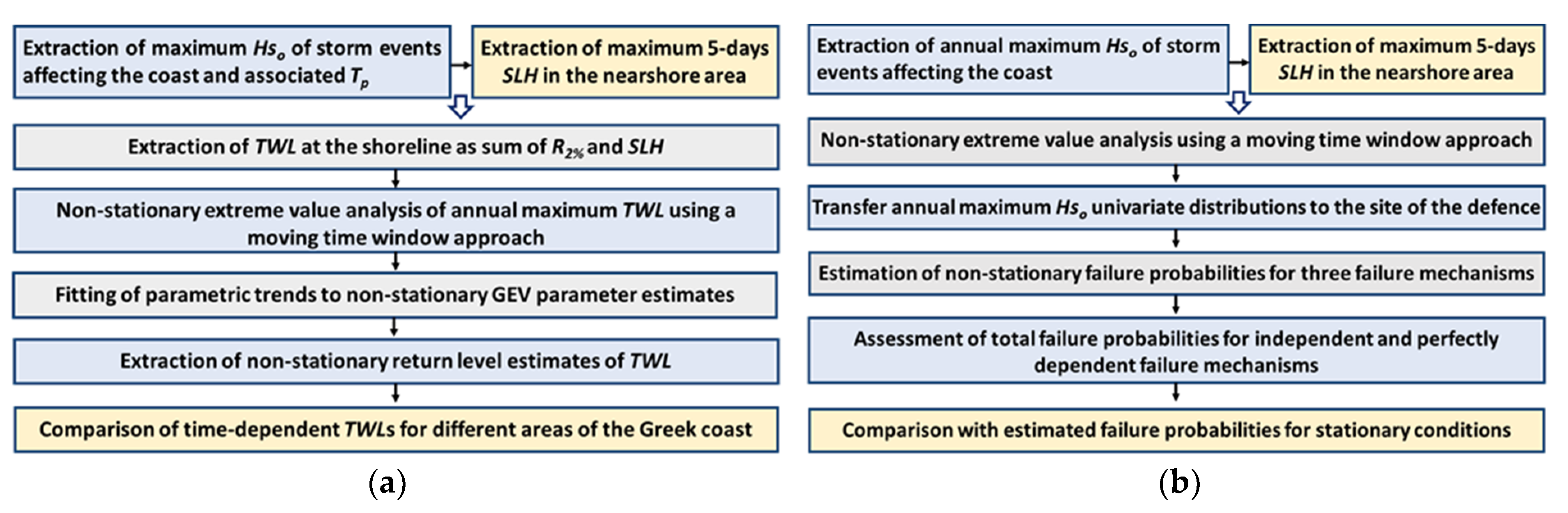
3.1. Estimation of Extreme Total Water Level on the Coast under Nonstationary Conditions

Coastal flooding, caused by the combined effect of high-water levels (storm surges and astronomical tides), MSL rise, and wave action of rough sea states can result from the combination of large values by more than one of its constituent processes. Therefore, a compound extreme TWL can be a combination of variables that are not necessarily extreme events themselves [25]. Moreover, it can be deduced that an extreme source is not equivalent to an extreme impact, according to the definition of compound events in the IPCC SREX report [74]. Based on this principle, the basic characteristic of a compound event, such as coastal flooding, is the importance of the extremeness of the impact rather than the individual components of the event [75]. In such previous works [24,76,77], a response function was defined (i.e., TWL incorporating the overtopping, run-up, etc.) as a measure of the impact that a coastal event may cause. This response function provided the sample of multivariate maxima used in hazard analysis. Therefore, in the present work, an impact-based definition of multivariate sea storm events is used, adopting a compound event approach to estimate extreme TWL at the shoreline. Deep-water significant wave heights and associated peak spectral wave periods, corresponding to offshore sea states affecting the coast, are primarily used to estimate the wave-induced run-up, R_2%, on the shoreline at selected coastal areas by means of the empirical formula [78]:

$$R_{2\%}=1.1\left(0.35\tan \beta {\left(H_s\cdot L_o\right)}^{\raisebox{1ex}{$1$}\!\left/ \!\raisebox{-1ex}{$2$}\right.}+\frac{{\left(H_s\cdot L_o\left(0.563{\tan }^2\beta +0.004\right)\right)}^{\raisebox{1ex}{$1$}\!\left/ \!\raisebox{-1ex}{$2$}\right.}}{2}\right)$$

(1a)

$$R_{2\%}=0.043{\left(H_s\cdot L_o\right)}^{\raisebox{1ex}{$1$}\!\left/ \!\raisebox{-1ex}{$2$}\right.}\mathrm{for}\xi <0.3$$

(1b)

where H_s [m] is the deep-water significant wave height, L_o [m] is the deep-water wave length associated to the peak spectral wave period T_p [s], $\tan \beta$ is the beach face slope, and ξ is the surf-similarity parameter (Iribarren number). The TWL at the shoreline results from adding the wave-induced run-up at the shoreline, R_2%, the sea level height due to storm surge, SLH, the MSL rise, MSLR, and the maximum astronomical tidal range, TR_max, at the selected study area:

$$TWL=R_{2\%}+SLH+MSLR+T{R}_{\max }$$

(2)

For all data available, annual maxima of the sum of the two stochastic components of TWL, R_2% and SLH, are extracted. In this study, a five-day window of SLH data was implemented, covering the estimated R_2% values by 2.5 days bilaterally. This was performed to estimate the largest possible SLH for each wave event, considering that storm events in the Mediterranean basin have a maximum duration of 120 h [26,71]. The extracted annual maxima of the aforementioned structure variable $\left(TW{L}_{stoch}=R_{2\%}+SLH\right)$ are then analyzed using univariate extreme value theory (EVT) to assess extremes of the TWL response. Considering the fact that climate change is one of the prominent causes of nonstationarity in the marine climate variables, and especially in their extremes, a nonstationary approach to estimate extreme TWLs at the shore is adopted in this work [79]. Thus, we incorporate the nonstationary version of the GEV distribution function, in which the three parameters, namely location μ, scale σ, and shape ξ are assumed to be time-varying [80]:

$$G\left(x\right)=\exp \left[-{\left\{1+\xi \left(t\right)\frac{\left(x-\mu \left(t\right)\right)}{\sigma \left(t\right)}\right\}}^{-1/\xi \left(t\right)}\right],1+\xi \left(t\right)\frac{\left(x-\mu \left(t\right)\right)}{\sigma \left(t\right)}>0$$

(3)

A fifty-year moving time window shifted by one year each time was implemented here to assess the nonstationary GEV parameters for the studied variable of TWL at the shoreline. The length of the moving window was assessed by means of a sensitivity analysis forming a trade-off between a short enough period for the assumption of stationarity to be satisfied for fitting extreme value distributions and an interval of adequate length to provide a good fit of the marginal distributions of the marine variables and to not alter their possible dependence structure [26]. The derived GEV parameter estimates correspond to the last year of each fifty-years period and are assessed using the method of L-moments [81,82].

Linear and nonlinear parametric trends are then fitted to the extracted GEV parameter estimates. Best-fitted models are selected using the Akaike Information Criterion (AIC) [83]:

$$AIC=-2\ln (L)+2p$$

(4)

and the Bayesian Information Criterion (BIC) [84]:

$$BIC=-2\ln (L)+p\ln (N)$$

(5)

where ln(L) is the log-likelihood, p is the number of estimated parameters in the model, and N is the sample size, as well as tests for statistical significance of the coefficients of the fitted trends. Nonlinear trends include polynomials of order lower than or equal to five. Statistically significant trends are judged using the Mann–Kendall test for linear trends and F- or t-tests for polynomial trends [26].

Nonstationary design TWLs are then defined as a conditional sum of extracted return level estimates of the structure variable (with or without the fitted parametric trends), astronomical tide, and MSL rise estimates at the selected coastal areas (Equation (2)). Confidence intervals for the studied return levels are assessed by applying a parametric bootstrap approach [85] for each of the 50-year moving time windows of the TWL extremes. One hundred bootstrap samples are created for each moving window, while up to fifth-degree polynomials are then fitted to the estimated mean values as well as to the 95% confidence intervals.

3.2. Analysis of Nonstationary Extreme Sea States at Port Areas or Harbour Sites

Port or harbor structures ensure that downtime risks (defined as the stoppage of operations within the protected basins due to malfunction of the protection system) are kept low. Such risks are a combination of the failure probability of a structure and its relevant impact, usually estimated as the product of the occurrence probability of the event and its consequences. Port or harbor downtime risks are considered to be crucial, especially for coastal areas characterized by high concentration of critical infrastructure and economic activities, and by high significance of seaport industry, short-sea shipping, and maritime transport and communications due to tourism, fishing, and other sea-related activities. The latter are determining factors of national economic performance, development, and regional growth. However, a large number of port and harbor structures worldwide are aging and have already exceeded their service lifetime. The abovementioned challenges, coupled with the general inception of a changing climate, are expected to increase exposure and vulnerability of engineered coastal areas to future risks. Hence, the functionality and safety of such structures have to be re-evaluated under climate change conditions and appropriate upgrading mitigation measures must be considered.

The boundary conditions for designing or evaluating the safety of port or harbor protection structures mainly include the marine hydraulic conditions at the defense site. Such hydraulic conditions are included in the estimation of the ultimate limit states (ULS) and serviceability limit states (SLS) of each protective structure separately. ULS are those associated with collapse or failure, also including loss of stability of the structure as a whole, leading to downtime of the protected basin, and are therefore associated with extreme marine conditions. SLS correspond to conditions, beyond which, specific service standards of a structure or structural member could no longer be met. Such conditions usually happen under excessive wave height within the protected basin, causing problems for standard operations [37].

To capture nonstationarity in the univariate marine extremes, a time-dependent GEV distribution described in Equation (3) was fitted to deep-water H_s annual maximum events [82]. To estimate the parameters of the nonstationary distributions, a 50-year length moving time window with an annual time step was used with the derived parameter estimates corresponding to the last year of each 50-year period. A five-day window of SLH was implemented, covering the annual maximum H_s values by 2.5 days bilaterally (see Section 3.1). Maximum values of SLH in the five-day windows were then also fitted by a time-dependent GEV distribution [82] (Equation (3)).

The abovementioned nonstationary univariate distributions for extreme H_s were then transferred to the site of the breakwater following an approach proposed by [28]. The latter is based on the assumption that H_s distributions in coastal waters reduce in the mean and in the standard deviation compared with the deep-water waves, so that their coefficient of variation remains constant:

$${\mathrm{cov}}_{cw}={\mathrm{cov}}_{dw}=\frac{stdev}{mean}=\frac{\frac{\sigma }{\xi }\sqrt{\left[\Gamma \left(1-2\xi \right)-{\Gamma }^2\left(1-\xi \right)\right]}}{\mu +\sigma \frac{\Gamma \left(1-\xi \right)-1}{\xi }}$$

(6)

where cov_cw and cov_dw is the coefficient of variation in coastal waters and deep waters, respectively, and Γ is the Gamma function. This assumption seems quite realistic for extreme waves, as their probability density function becomes narrower and is shifted toward smaller values as they propagate in coastal waters, while its shape does not undergo any significant changes. This procedure, which also considers design quantities of the existing structure, was implemented for each moving window to extract time-dependent estimates of all GEV parameters in the study area.

3.3. Assessment of Nonstationary Failure Probabilities of Rubble Mound Breakwaters

In our approach, the principal failure mechanisms (FM) of conventional rubble mound breakwaters include: (1) failure or instability of the windward armor layer; (2) failure of the leeward slope; (3) scouring of the toe; (4) excessive overtopping; (5) the slip cycle; (6) sliding and tilting of existing superstructures; and (7) excessive settlement. These are slightly different yet inclusive of and more than the ones proposed by [56], namely displacement of units from the main armor layer (FM1), displacement of the superstructure (FM6), soil deformation, and core erosion (indirectly included in FM3 and FM7). The present work focuses on ULS failure of the studied structure resulting to port downtime and examines three failure modes as the main types of instability under extreme marine conditions, treating the port structure as a whole and neglecting subsystem breakdowns [56]. These failure mechanisms include instability of the windward primary armor layer (FM1), excessive overtopping (FM4), and scouring of the breakwater toe (FM3).

Reliability analysis hinges on the use of the probability of failure, P_f, as a measure of the structure’s performance. The reliability function, Z, for a certain limit state is defined as the difference between the resistance of the structure, R, and the load, S, it is exposed to. The failure domain is defined for Z ≤ 0:

$$P_f=P\left(Z\le 0\right)=P\left(S\ge R\right)$$

(7)

Reliability functions contain variables of the marine climate at the windward side of the breakwater, as well as variables describing geometrical and material properties of the studied structure. Level II reliability methods were used in this work to assess time-dependent P_f for all three limit states considered. These are most suitable in our case, as the project objectives need to follow the adaptation of total costs to limited budgetary resources and the need for financial sustainability of any necessary investment, while minimizing the uncertainty and maximizing the reliability of the constructed structure for a viable decision-making process based on acceptable risk levels by OLA S.A. [56]. Variables included in the limit states are first normalized and then the reliability function Z is linearized at an appropriately defined design point of the failure space. The distance from the origin of the transformed coordinate system to the failure space, which is described by a linear function (or edge of the failure area in case of multiple linearized functions Z = 0), is referred to as the reliability index, β [86]:

$$\beta ={\min }_{Z=0}\left(\sqrt{U^2{}_1+U^2{}_2}\right)$$

(8)

and the failure probability is therefore defined as a function of β:

$$P_f=\Phi \left(-\beta \right)$$

(9)

To extract the total failure probability for a particular structure, a fault tree is usually created giving a logical succession of all events leading to port/harbor downtime, containing both ULS and SLS (if any). Dependencies between these failure mechanisms should also be considered to extract accurate estimates of expected total failure probabilities. In this study, dependencies of the three ULS considered are not known, and therefore the lower and upper bound of the total failure probability was defined as the probability of fully dependent and mutually exclusive events, respectively:

$$\max \left(P_f\left(1\right),P_f\left(2\right),P_f\left(3\right)\right)\le P_f{}^{series}\le P_f\left(1\right)+P_f\left(2\right)+P_f\left(3\right)$$

(10)

The reliability function for hydraulic stability of a windward primary armor layer composed of Accropodes is based on the stability formula of Van der Meer [87], using a safety factor of 1.5:

$$Z_{stability}=2.5\cdot \Delta \cdot D_n-H_{su}$$

(11)

here,

$$\Delta =\left(\frac{{\rho }_{ac}}{{\rho }_w}\right)-1$$

(12)

and ρ_ac and ρ_w are the Accropode and water densities [ton/m³], D_n [m] is the characteristic diameter of armour stone units, and H_su [m] is the significant wave height in front of the studied breakwater corresponding to its ULS.

The reliability function for excessive wave overtopping is based on the following formula [88]:

$$Z_{overtopping}=q-0.2\cdot C_r\cdot \exp \left(-\frac{2.3\cdot R_c}{{\gamma }_f\cdot H_{su}}\right)\sqrt{g\cdot H_{su}^3},C_r=3.06\cdot \exp \left(-\frac{B}{H_{su}}\right)$$

(13)

with

$$R_c=H_{crest}-MSLR-T{R}_{\max }-SLH$$

(14)

where q [m²/s] is the maximum allowable overtopping discharge, C_r is the reduction factor due to effect of armoured crest berm of width B [m], γ_f is the influence factor for crest armour units, and R_c [m] is the freeboard height resulting when subtracting the sum of the MSL rise, MSLR [m], the maximum tidal range, TR_max [m], and the storm surge, SLH [m], from crest level height, H_crest [m].

The reliability function for toe stability is based on the formula [89]:

$$Z_{scouring}=\left(0.24\frac{h_t}{D_{n50}}+1.6\right)\cdot N_{od}^{0.15}\cdot \Delta \cdot D_{n50}-H_{su}$$

(15)

$$h_t=d+MSLR+T{R}_{mean}+SLH$$

(16)

where h_t [m] is the total water depth at the breakwater toe, D_n50 [m] is the characteristic diameter of toe elements, N_od is the number of displaced units within a strip with width D_n50, and d [m] is the depth of the water column from MSL to breakwater toe.

4. Results

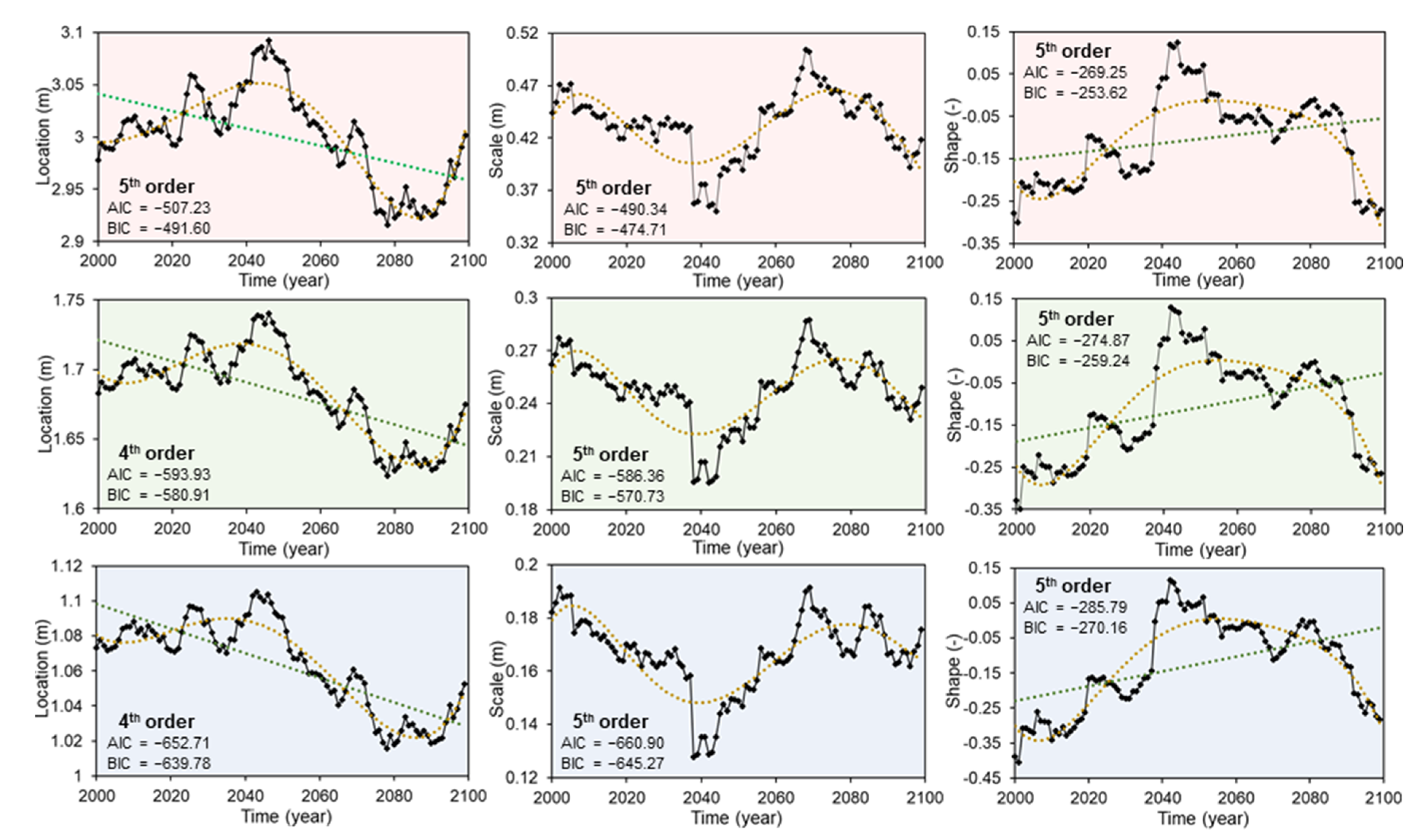
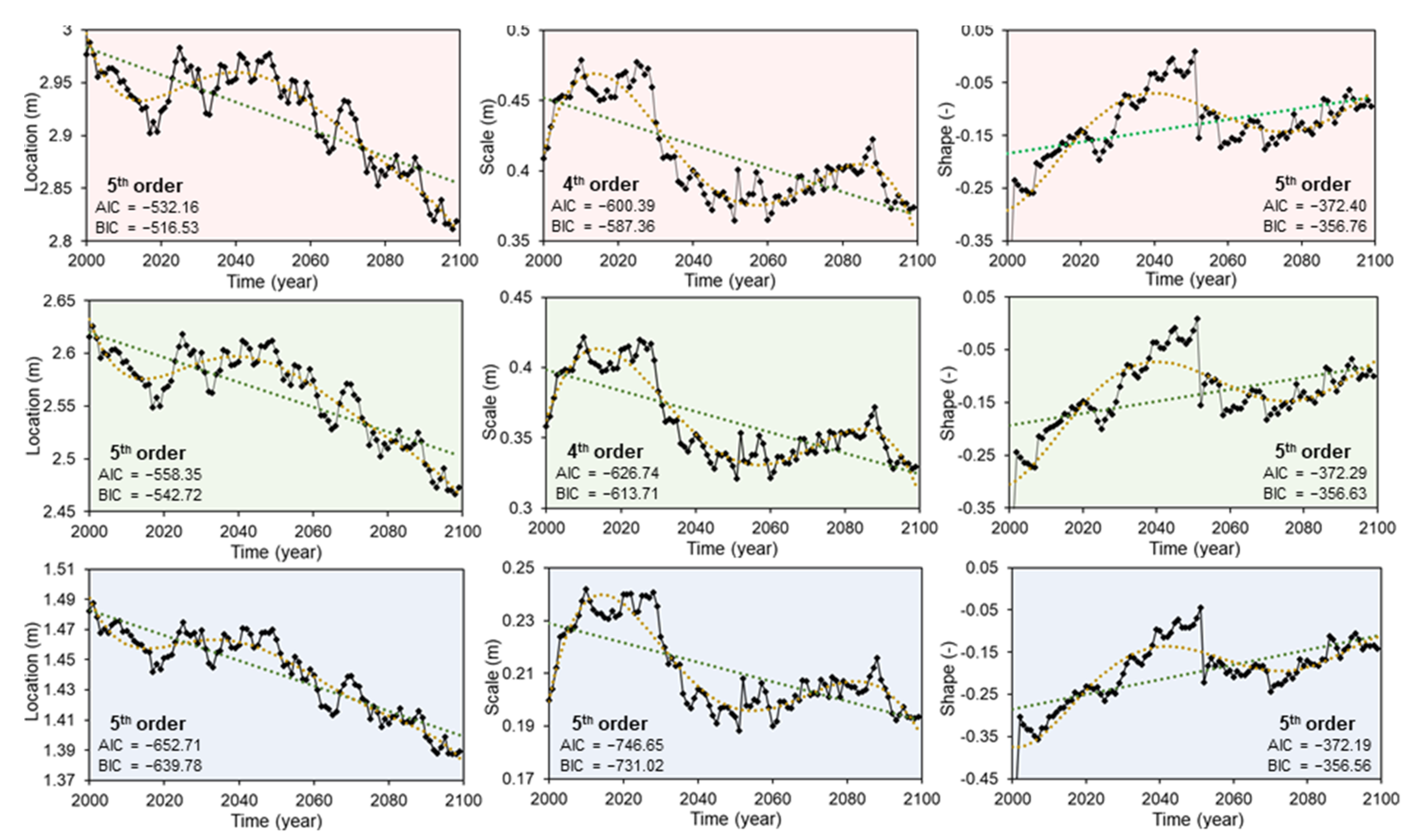
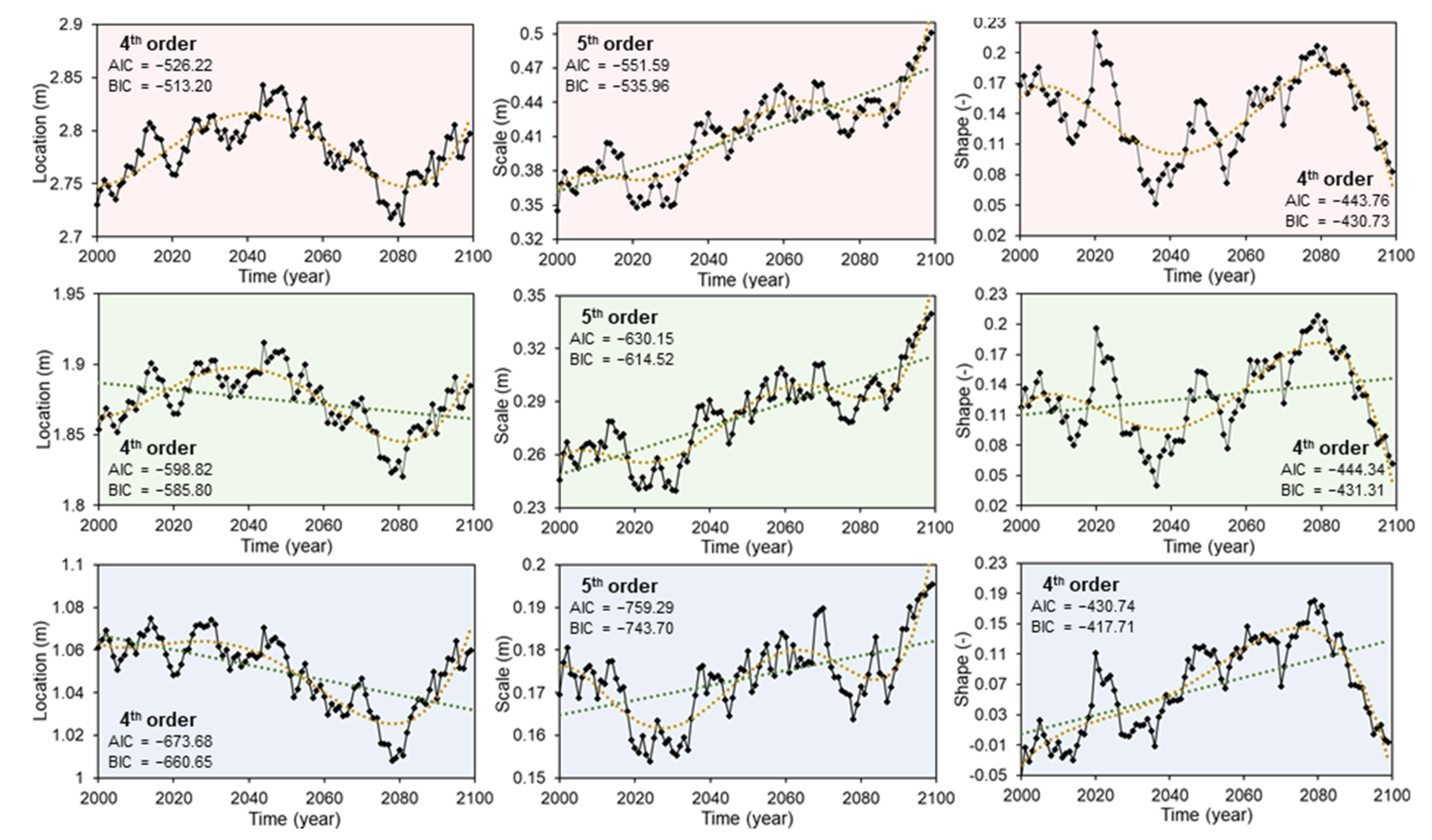
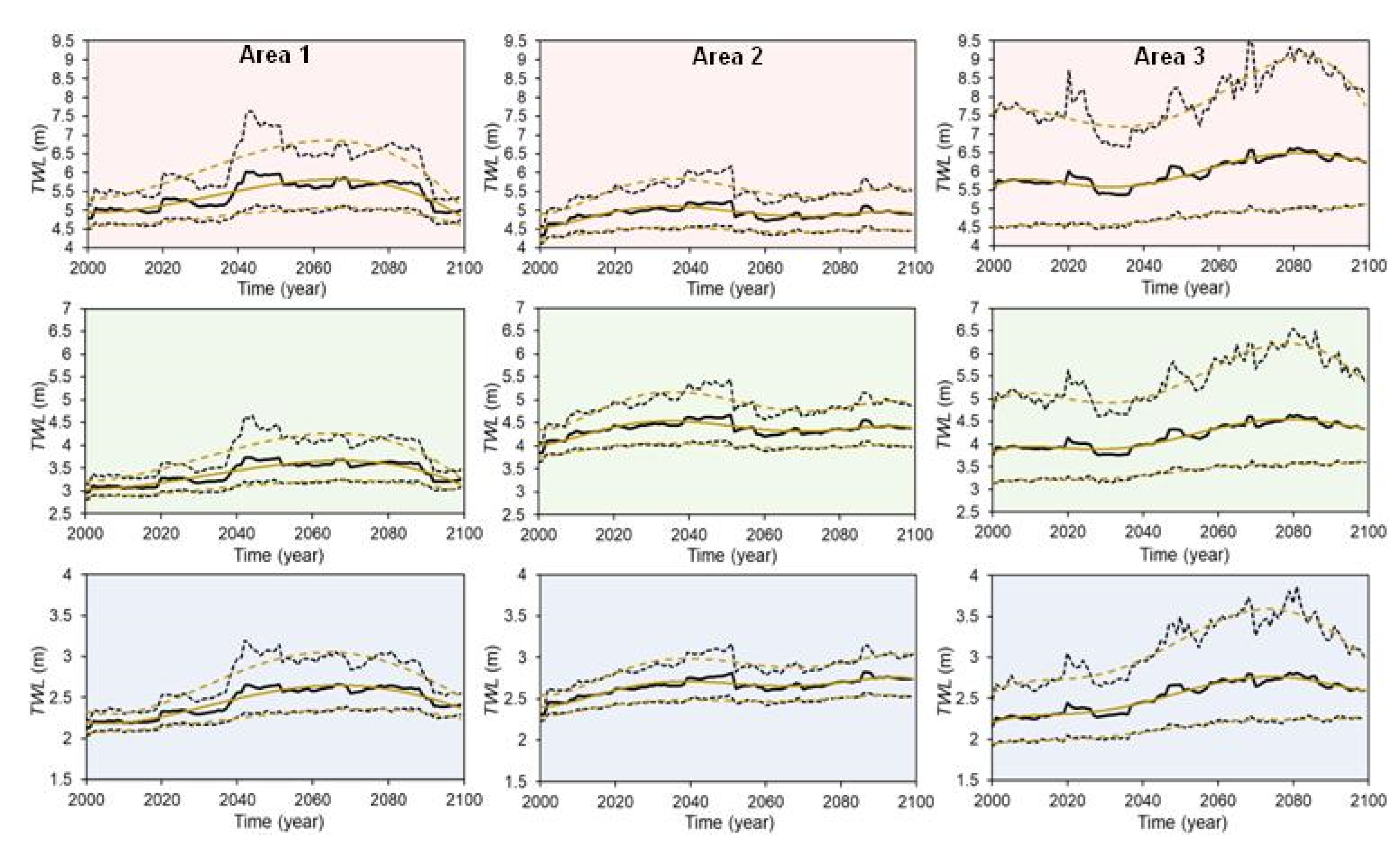
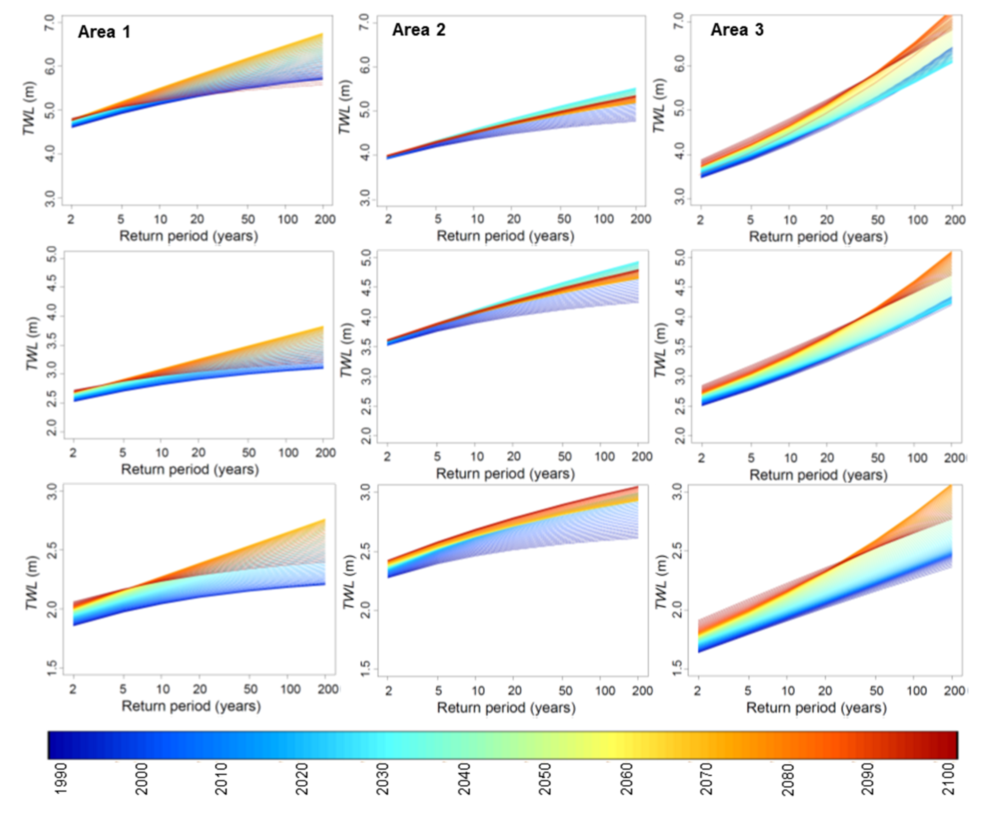
4.1. Nonstationary Extreme Total Water Levels on the Greek Coastal Zone

The nonstationary analysis of $TW{L}_{stoch}$ extremes using 50-year moving time windows for all selected cross-shore profiles including the maximum, the minimum, and a slope close to the median in all three study areas (see Section 2) resulted in obtaining time-dependent estimates of GEV parameters (location, scale, and shape) from 2000 to 2100. All parameter estimates were obtained using the L-moments approach. Figure 3 presents such estimates for the selected cross-shore profiles, including a maximum slope 17.1% (first row), a slope 7.5% close to the median of the selected profile sections (second row) and a minimum slope 1.2% (third row), at the coastal area of Alexandroupoli in the Thracian Sea (Area 1). Similar plots are presented in Figure 4 and Figure 5 for the coastal areas of Eresos in the east-central Aegean Sea (Area 2) and Iraklion in the Cretan Sea (Area 3), respectively. Figure 4 includes nonstationary GEV parameter estimates for a cross-shore profile with a maximum slope of 16.2% (first row), a slope 11.6% (second row) close to the median value of the selected profiles in the area, and a minimum slope of 5.7% (third row). The respective profile slopes in Figure 5 correspond to a maximum value of 14.5% (first row), a median of 8.5% (second row) and a minimum value of 3.0% (third row). Statistically significant linear trends (5% significance level), as well as best-fitted nonlinear trends for all parameters are also shown in Figure 3, Figure 4 and Figure 5. In the present work, the maximum order of the fitted polynomial trends was set equal to five. The best fitted polynomial trends were selected based on minimizing the AIC and the BIC (Equations (4) and (5)). In cases where minimum values of the two criteria do not coincide, the model which provides the lowest BIC value is selected, provided that this criterion penalizes the log-likelihood more, avoiding overparameterization of the fitted trends.

The results presented in Figure 3, Figure 4 and Figure 5 for the entire range of cross-shore profile slopes examined in each study area reveal that even if the magnitude of the mean and variance of the distribution of TWL extremes increases with increasing beach profile slope, its tail behavior remains almost unchanged. In particular, the location and scale parameters of the fitted nonstationary GEV models increase with increasing beach face slope, even though they exhibit similar variations in the studied time interval. The shape parameter of the fitted distributions, which in fact determines the tail behavior of the fitted models, presents very slight changes with the three different profile slopes in each area. Some differences are however detected in the first years of the simulation period for the study site of Iraklion. Minor changes in TWL extremes’ tail behavior with profile slope can be partly attributed to the formula used to estimate the wave-induced run-up on the shoreline (Equation (1) [78]). The range of beach slope, tanβ, values do not seem to be large enough to significantly influence the tail behavior of extreme R_2%. Moreover, the Aegean Sea is a wave-dominated marginal basin in terms of coastal flooding, thus it seems reasonable for the tail behavior of TWL extremes to be mainly determined by the wave run-up. Therefore, the best-fit distribution to TWL extremes does not change significantly (with beach profile slope) in its skewness but shifts only in its mean and variance.

In all three study sites and for the majority of the selected profiles, the fitted nonstationary models indicate both heavy-tailed (lower-bounded distributions with positive shape parameter) and short-tailed (upper-bounded distributions characterized by negative shape parameter) intervals. Heavy-tailed distributions assessed for a number of 50-year intervals in all three study areas are not that common in studies on extreme values of marine variables such as wave heights and storm surges, largely due to physical constraints. However, the study of TWL_stoch, which incorporates the effects of a response variable, R_2%, and nearshore SLH, combined with climate change impacts on the primary variables of wave height and storm surge, can possibly support such findings. Heavy-tailed distributions are rather dominant for the study site of Iraklion (Area 3) in the southern Aegean Sea. They are furthermore confined to the most energetic part of the studied time interval (around the mid-century) for the coastal area of Alexandroupoli (Area 1) and are rather limited for the coastal area of Eresos (Area 2). Results of TWL, and thus the subsequent flooding hazard, seem to be more correlated to T_p than to H_s, since the run-up (major contributor to TWL) parameterization of Stockdon et al. [78] is highly dependent on random wave peak periods in comparison with significant wave heights; R_2% depends on the square-root of H_s while it is analogous to the first power of T_p, as L_o = gT_p²/2π. This fact corresponds to cases of long wave period sea-states in the southern Aegean with wave heights able to drive extreme TWLs. This might be the case due to the lower dependency of H_s − T_p pair in the specific region [26], and the fact that in Area 3 generally higher T_p values are reported compared to the other two Areas (1–2) of the Aegean. In the southern part of the Aegean basin, the existence of a dense island cluster (Cyclades) may be responsible for this effect, due to diffraction of long waves having prominent impacts on H_s extremes, while allowing for larger T_p values to occur. Moreover, some pairs of longer (high T_p and L_o values) but smaller (lower H_s values) waves that could theoretically drive larger flooding might exist, but do not qualify as efficient wave storm events, either because of their insufficient short duration (<6 h) or ineffective directionality. The latter also applies to the central Aegean (Area 2) of Lesvos Island too, which is more protected from incident wave action originating from the southern and western sectors, due to the topographical peculiarities in the region, compared to Area 1.

Statistically significant linear trends have been detected in almost all GEV parameters for all three study areas. The only exceptions are the scale parameter for Area 1 for all three profile slopes considered and the location and shape parameters for Area 3 for the maximum cross-profile slope. Such trends are decreasing for the location and increasing for the shape parameter in all areas, identifying distribution functions with progressively lower means and heavier tails during the future period. GEV distribution functions seem to present progressively lower variances (represented by the scale parameter) in the future in Area 2, and higher ones in Area 3.

Statistically significant polynomial trends have been also detected in all parameters of the GEV fitted to TWL_stoch for all three study areas. In the present work the maximum order of the fitted polynomial trends was set equal to five. All resulting polynomial trends are of order four or five, identifying quite high variability of the GEV parameter estimates with time in all study areas. Larger differences in variations over time among the study coastal areas are observed for the scale parameter, which shrinks or stretches the TWL distribution and the shape parameter, which dictates its limiting behavior. In Area 1 the scale parameter presents a bimodal behavior, peaking at the beginning and after the middle of the 21st century, while during the latter period the shape parameter presents its highest values. In Area 2 the scale parameter decreases considerably after 2020, while highest values of the shape parameter are obtained around the middle of the 21st century. Finally, in Area 3, the scale parameter presents an increasing trend, while heavy tails characterize the distribution of TWL throughout the 21st century, as mentioned previously.

Within a nonstationary context, which is indeed imposed by climate change, TWL return levels could not be interpreted as events with a certain exceedance probability in a defined interval but are rather conceived as quantiles of the distribution of TWL in each year, namely in the last year of each 50-years period. Figure 6 presents time-dependent 100-years return levels of TWL (Equation (2)) for the period 2000–2100 for all cross-shore profiles examined in all three study areas. Most likely 100-years return levels are presented, together with their associated 95% confidence intervals estimated using a parametric bootstrap approach (see Section 3). Figure 6 also includes 100-years most likely and 95% confidence interval TWL estimates assessed by considering best-fitted nonlinear parametric trends for all GEV parameters. It should be noted here that Figure 3, Figure 4 and Figure 5 present time variations of GEV parameters in all three study areas (Alexandroupoli, Eresos, Iraklion), used to produce time dependent return level estimates of TWL_stoch (most likely values and 95% confidence intervals) for a return period of 100 years. MSL rise in each year in 2000–2100 and maximum astronomical tidal range, TR_max, in each study area are then added to the extracted TWL_stoch 100-year estimates to produce final time-dependent estimates of 100-year TWL.

In each of the three areas considered the main contributor to the differences in TWL estimates is the wave-induced run-up, R_2%, which depends critically on the beach face slope and is calculated using Equation (1). TWL extremes in Area 1 appear to increase in the second half of the 21st century, while uncertainty almost doubles in this interval (apart from the last ten years), with respect to the period 2000–2040. Considering nonlinear trends in GEV parameters, most likely TWL extremes peak in the interval 2065–2070 to the value of 3.6 m (from 2.7 m to 6.0 m considering minimum and maximum slope). In Area 2, extreme TWLs seem to increase in the first half of the 21st century and decrease in the second one, presenting their highest values of 4.7 m around the middle of the century (from 2.7 m to 5.3 m considering minimum and maximum slope). When including parametric trends in the GEV parameters, highest values of 100-years TWL estimates appear around 2035. In Area 3, extreme TWLs present their highest values of 4.6 m around 2080 (from 2.8 m to 6.6 m considering minimum and maximum slope), appearing highly uncertain throughout almost the entire study period. Variability of most likely 100-years TWL estimates in all study areas exceeds 20% in the 21st century, while it increases to more than 35% when upper 95% confidence intervals are considered.

Figure 7 presents TWL return level estimates from 2000 to 2100 corresponding to return periods from 2 to 200 years in the three coastal areas of the northern (Area 1), central (Area 2), and southern (Area 3) Aegean Sea. Estimates shown were produced for all cross-shore profile slopes (maximum, median, minimum), considering best-fitted nonlinear parametric trends in the GEV parameters.

In Area 1, TWL return level estimates present an increasing trend until 2065–2070 and a decreasing trend afterwards, for the entire range of probabilities considered. Differences are more pronounced for high return periods. The decrease in TWL values is quite sharp (especially for high return periods), leading to short (light)-tailed distributions in the last thirty years of the 21st century. In Area 2, TWL return level estimates associated with low probabilities of occurrence present an abrupt increase in the first half of the 21st century and decrease slightly afterwards. Short-tailed GEV distribution functions are assigned to the entire study period, enabling the extraction of design values of the response for different impact studies. In Area 3, TWL return level estimates progressively increase during the period 2000–2080. Extreme TWLs are fitted to GEV distribution functions with progressively heavier tails, turning to upper-bounded distribution functions in the last twenty years of the 21st century. From Figure 7, it is again evident that the cross-shore profile slope in a defined study area does not significantly affect the tail behavior of TWL extremes.

4.2. Nonstationary Failure Probabilities of Rubble Mound Breakwaters

The nonstationary GEV distribution was first fitted to extreme deep-water H_s (H_so) and nearshore SLH close to the port of Alexandroupoli (Figure 2) and parameters of the fitted 50-year windows were estimated using L-moments [81,82]. Figure 8 presents time-dependent estimates of 100-years return levels of H_so and SLH for the selected study site, together with their associated 95% confidence intervals estimated using a parametric bootstrap approach (see Section 3).

H_s return level estimates present an increasing trend in the first half of the 21st century, with their maximum values in 2040–2055. A second peak in H_s extremes appears around 2065–2070, while H_s decreases rapidly at the end of the century. Most probable estimates of H_s vary more than 33% within the 21st century, while predictions in the mid-century appear highly uncertain (very wide 95% confidence intervals). GEV distributions of deep-water H_s extremes have been then transferred to the studied breakwater site (see Section 3.2). SLH extremes at the breakwater site show quite similar variation to the respective deep-water H_s estimates. They present an evident increasing trend in 2020–2040, and a decreasing one in 2070–2100. Two peaks in SLH extremes can be distinguished, around 2035–2040 and 2065, while predictions in 2040–2070 are characterized by increased uncertainty.

Figure 9 presents nonstationary estimates of the location and scale parameters of the fitted GEV models to extreme deep-water H_s (H_so) and H_s transferred at the breakwater site. The shape parameter of the models in deep water conditions is assumed to remain unaltered when waves propagate nearshore and varies in the interval (−0.22, 0.20), taking its highest values in 2020–2030 and 2040–2055.

The GEV location parameter decreases significantly when the distribution of deep-water H_s is transferred to the studied breakwater site, with differences ranging between 10% and 68%. The location of the H_s distribution at the breakwater site presents an evident increasing trend in the first half of the 21st century, while obtaining its highest value in the last decade of the century where the shape parameter of the GEV distribution is highly negative. The GEV scale parameter also decreases when H_s propagates nearshore, verifying the assumption of narrower probability density functions at coastal waters. Due to assumed stability in the coefficient of variation in coastal and deep waters (Equation (6)), differences in the scale parameter are similar to those in the location parameter. It should also be noted that the scale parameter preserves its variability at coastal waters, apart from the last ten years of the study interval.

The left panel of Figure 10 presents nonstationary P_f estimates for the three selected failure mechanisms (see Section 3.3). In Equation (13) the maximum allowable overtopping discharge q = 5 L/m² [17], while the number of displaced units in Equation (15) is considered N_od = 0.5, corresponding to negligible damages at the breakwater toe. The right panel of Figure 10 presents estimates of total failure probability, P_ftotal, considering the three ULS as mutually exclusive (also shown in the left panel of Figure 10) or perfectly dependent (total failure probability coincides with failure probability extracted for the overtopping failure mechanism). It also includes P_ftotal estimates from the series of 150 (1951–2100) and 100 (2001–2100) years, considering stationarity of marine conditions. Lower and upper bounds of these intervals correspond to perfect dependence or mutual exclusivity of ULS. It should be noted here that total failure probabilities estimated assuming independent ULS are really close to those of mutually exclusive ones.

Estimated probabilities for all failure mechanisms present a bimodal behavior, showing discrete peaks in the intervals of maximum H_s. Therefore, P_f of all three mechanisms vary considerably within the 21st century. Maximum values of failure probabilities are estimated 0.0072, 0.0123, and 0.0097 for the primary armor layer stability, the overtopping, and the toe stability failure mechanism, respectively. Excessive overtopping seems to be the governing failure mechanisms for the entire study period, followed by scouring of the breakwater toe and by instability of primary armor layer of the structure. The highest P_f correspond to return periods of 81, 104, and 140 years, for overtopping, scouring of the breakwater toe and instability of its primary armor layer, respectively. It should be noted that even if the structure can be considered quite safe for present marine conditions, since P_f for all failure mechanisms correspond to return periods of less than 1000 years in the first twenty years of the 21st century, it seems to be exposed to severe marine conditions in the future. Considering the excessive overtopping ULS, P_f in the interval 2065–2070 are estimated higher compared to the respective ones in the middle of the century, identifying the significant contribution of MSLR and SLH in determining failure conditions.

The highest total failure probabilities correspond to return periods of 36 and 81 years, for perfectly dependent or mutually exclusive ULS, respectively. From Figure 10 it is evident that the stationarity assumption significantly underestimates P_ftotal. This underestimation reaches 82% and 64% when failure probabilities are estimated for 150 and 100 years, respectively.

5. Conclusions

In this study, multivariate extreme sea states (storm waves and surges) at selected areas of the Greek coastal zone, representing a possible realization of the future marine climate, are statistically treated via EVT, considering nonstationarity on time scales longer than the seasonal or interannual scale, possibly attributed to climate change. Furthermore, they are combined with other sources of the coastal flooding hazard (i.e., astronomical tides and MSL rise) allowing for a robust derivation of extreme values, which is mainly focused on the associated response function of the TWL in coastal areas of the Aegean Sea. This hopefully allows for safer estimations of the coastal flooding hazards, more reliable design values for coastal protection works, and more efficient management of the coastal zone.

The nonstationary analysis of the response function of TWL revealed statistically significant nonlinear trends in all GEV parameters and identified quite a high variability in its estimates in all study areas. TWL peaks appearing after 2060 in northern Aegean Sea imply the rise of extreme southerly winds in the area towards the middle of the 21st century and beyond [63]. Progressive increase of TWL extremes in southern Aegean Sea could be possibly combined with a mild rise of northerly extreme winds after the first half of the 21st century detected in the Aeolian patterns [26]. Finally, the projected significant increase in extreme Etesians (i.e., local strong meridional winds called “Meltemia” [90]) in the first half of the 21st century could possibly explain peaks in $TWL$ extremes in the central Aegean Sea during this period.

Furthermore, failure probabilities of an indicative rubble mound breakwater protecting a Greek port against increasing future marine hazards and related escalating exposure to downtime risks are also estimated within a nonstationary extreme value analysis framework. The results concern time-dependent P_f estimates for three main ULS, which are intercompared and used to determine future periods of increased vulnerability of the studied structure to extreme marine hazards. Excessive overtopping ULS seems to be the most critical for the collapse of the studied defense. This failure mechanism identifies a period around 2065–2070, with the highest P_f, where all variables of the marine climate (H_s, MSLR and SLH) have a significant contribution to port downtime. Total failure probabilities are quite high for the future periods 2040–2055 and 2065–2070, with the highest values corresponding to a return period of 36 years for mutually exclusive ULS.

Conclusively, estimating P_ftotal within a nonstationary reliability framework assists in avoiding underestimation of future marine hazard effects on port and harbor structures. It should be noted that only selected ULS are considered in the present work. Excessive wave height inside the port/harbor basin during normal weather conditions causes port downtime without severe collapse of defense structures, and thus can be regarded as Serviceability Limit State (SLS). Such limit states can significantly affect P_ftotal of Greek ports and harbors.

References

1. IPCC. Climate Change 2007: The Scientific Basis, Contribution of Working Group I to the Fourth Assessment Report of IPCC; Cambridge University Press: Cambridge, NY, USA, 2007. [Google Scholar]
2. IPCC. Managing the Risks of Extreme Events and Disasters to Advance Climate change Adaptation. In A Special Report of Working Groups I & II of IPCC; Cambridge University Press: Cambridge, NY, USA, 2012. [Google Scholar]
3. IPCC. Climate Change 2013: The Physical Science Basis, Contribution of Working Group I to the Fifth Assessment Report of IPCC; Cambridge University Press: Cambridge, NY, USA, 2014. [Google Scholar]
4. Marcos, M.; Tsimplis, M.N. Coastal sea level trends in Southern Europe. Geophys. J. Int. 2008, 175, 70–82. [Google Scholar] [CrossRef] [Green Version]
5. Somot, S.; Sevault, F.; Déqué, M.; Crépon, M. 21st century climate change scenario for the Mediterranean using a coupled atmosphere–ocean regional climate model. Glob. Planet Chang. 2008, 63, 112–126. [Google Scholar] [CrossRef] [Green Version]
6. Carillo, A.; Sannino, G.; Artale, V.; Ruti, P.M.; Calmanti, S.; Dell’Aquila, A. Steric sea level rise over the Mediterranean Sea: Present climate and scenario simulations. Clim. Dyn. 2012, 39, 2167–2184. [Google Scholar] [CrossRef]
7. Tsimplis, M.N.; Calafat, F.M.; Marcos, M.; Jordá, G.; Gomis, D.; Fenoglio-Marc, L.; Struglia, M.V.; Josey, S.A.; Chambers, D.P. The effect of the NAO on sea level and on mass changes in the Mediterranean Sea. J. Geophys. Res. Ocean. 2013, 118, 944–952. [Google Scholar] [CrossRef] [Green Version]
8. Adloff, F.; Somot, S.; Sevault, F.; Jordà, G.; Aznar, R.; Déqué, M.; Herrmann, M.; .Marcos, M.; Dubois, C.; Padorno, E.; et al. Mediterranean Sea response to climate change in an ensemble of twenty first century scenarios. Clim. Dyn. 2015, 45, 2775–2802. [Google Scholar] [CrossRef]
9. Μéndez, F.J.; Menéndez, Μ.; Luceño, A.; Losada, Ι.J. Estimation of the long-term variability of extreme significant wave height using a time-dependent Peak Over Threshold (POT) model. J. Geophys. Res. 2006, 111. [Google Scholar] [CrossRef]
10. Lionello, P.; Cogo, S.; Galati, M.B.; Sanna, A. The Mediterranean surface wave climate inferred from future scenario simulations. Glob. Planet Chang. 2008, 63, 152–162. [Google Scholar] [CrossRef]
11. Benetazzo, A.; Fedele, F.; Carniel, S.; Ricchi, A.; Bucchignani, E.; Sclavo, M. Wave climate of the Adriatic Sea: A future scenario simulation. Nat. Hazard Earth Syst. Sci. 2012, 12, 2065–2076. [Google Scholar] [CrossRef] [Green Version]
12. Casas-Prat, M.; Sierra, J.P. Projected future wave climate in the NW Mediterranean Sea. J. Geophys. Res. Ocean. 2013, 118, 3548–3568. [Google Scholar] [CrossRef]
13. Galiatsatou, P.; Prinos, P. Analysing the effects of climate change on wave height extremes in the Greek Seas. In Proceedings of the 11th International Conference on Hydroscience & Engineering (ICHE 2014), Hamburg, Germany, 28 September–2 October 2014; Lehfeldt, R., Kopmann, R., Eds.; Bundesanstalt für Wasserbau: Karlsruhe, Germany, 2014; pp. 773–781, ISBN 978-3-939230-32-8. [Google Scholar]
14. Galiatsatou, P.; Prinos, P. Estimating the effects of climate change on storm surge extremes in the Greek Seas. In Proceedings of the 36th IAHR World Congress, The Hague, The Netherlands, 28 June–3 July 2015. [Google Scholar]
15. Makris, C.; Galiatsatou, P.; Prinos, P.; Anagnostopoulou, C.; Kapelonis, Z.; Kombiadou, K.; Velikou, K.; Gerostathis, T.; Androulidakis, Y.; Vagenas, C.; et al. Climate Change Effects on the Marine Characteristics of the Aegean and Ionian Seas. Ocean Dyn. 2016, 66, 1603–1635. [Google Scholar] [CrossRef]
16. Snoussi, M.; Ouchani, T.; Niazi, S. Vulnerability assessment of the impact of sea-level rise and flooding on the Moroccan coast: The case of the Mediterranean eastern zone. Estuar. Coast Shelf Sci. 2008, 77, 206–213. [Google Scholar] [CrossRef]
17. Sánchez-Arcilla, A.; Jiménez, J.A.; Valdemoro, H.I.; Gracia, V. Implications of climatic change on Spanish Mediterranean low-lying coasts: The Ebro delta case. J. Coast. Res. 2008, 24, 306–316. [Google Scholar] [CrossRef]
18. Sanó, M.; Jiménez, J.A.; Medina, R.; Stanica, A.; Sanchez-Arcilla, A.; Trumbic, I. The role of coastal setbacks in the context of coastal erosion and climate change. Ocean Coast Manag. 2011, 54, 943–950. [Google Scholar] [CrossRef]
19. Alvarado-Aguilar, D.; Jiménez, J.A.; Nicholls, R.J. Flood hazard and damage assessment in the Ebro Delta (NW Mediterranean) to relative sea level rise. Nat. Hazards 2012, 62, 1301–1321. [Google Scholar] [CrossRef]
20. Fatorić, S.; Chelleri, L. Vulnerability to the effects of climate change and adaptation: The case of the Spanish Ebro Delta. Ocean Coast Manag. 2012, 60, 1–10. [Google Scholar] [CrossRef]
21. Villatoro, M.; Silva, R.; Méndez, F.J.; Zanuttigh, B.; Pan, S.; Trifonova, E.; Losada, I.J.; Izaguirre, C.; Simmonds, D.; Reeve, D.; et al. An approach to assess flooding and erosion risk for open beaches in a changing climate. Coast. Eng. 2014, 87, 50–76. [Google Scholar] [CrossRef] [Green Version]
22. Karambas, T.; Galiatsatou, P.; Prinos, P. Modeling of climate change effects on coastal erosion. In Proceedings of the 11th International Conference on Hydroscience & Engineering (ICHE 2014), Hamburg, Germany, 28 September–2 October 2014; Lehfeldt, R., Kopmann, R., Eds.; Bundesanstalt für Wasserbau: Karlsruhe, Germany, 2014; pp. 591–598, ISBN 978-3-939230-32-8. [Google Scholar]
23. Kokkinos, D.; Prinos, P.; Galiatsatou, P. Assessment of coastal vulnerability for present and future conditions in coastal areas of the Aegean Sea. In Proceedings of the 11th International Conference on Hydroscience & Engineering (ICHE 2014), Hamburg, Germany, 28 September–2 October 2014; Lehfeldt, R., Kopmann, R., Eds.; Bundesanstalt für Wasserbau: Karlsruhe, Germany, 2014; pp. 1043–1051, ISBN 978-3-939230-32-8. [Google Scholar]
24. Serafin, K.A.; Ruggiero, P. Simulating extreme total water levels using a time-dependent extreme value approach. J. Geophys. Res. Ocean. 2014, 119, 6305–6329. [Google Scholar] [CrossRef] [Green Version]
25. Serafin., K.A.; Ruggiero, P.; Stockdon, H.F. The relative contribution of waves, tides, and nontidal residuals to extreme total water levels on U.S. West Coast sandy beaches. Geophys. Res. Lett. 2017, 44, 1839–1847. [Google Scholar] [CrossRef]
26. Galiatsatou, P.; Makris, C.; Prinos, P.; Kokkinos, D. Nonstationary joint probability analysis of extreme marine variables to assess design water levels at the shoreline in a changing climate. Nat. Haz. 2019, 98, 1051–1089. [Google Scholar] [CrossRef]
27. Becker, A.; Inoue, S.; Fischer, M.; Schwegler, B. Climate change impacts on international seaports: Knowledge, perceptions, and planning efforts among port administrators. Clim. Chang. 2012, 110, 5–29. [Google Scholar] [CrossRef]
28. Suh, K.D.; Kim, S.W.; Kim, S.; Cheon, S. Effects of climate change on stability of caisson breakwaters in different water depths. Ocean. Eng. 2013, 71, 103–112. [Google Scholar] [CrossRef]
29. Sekimoto, T.; Isobe, M.; Anno, K.; Nakajima, S. A new criterion and probabilistic approach to the performance assessment of coastal facilities in relation to their adaptation to global climate change. Ocean. Eng. 2013, 71, 113–121. [Google Scholar] [CrossRef]
30. Isobe, M. Impact of global warming on coastal structures in shallow water. Ocean. Eng. 2013, 71, 51–57. [Google Scholar] [CrossRef]
31. Sánchez-Arcilla, A.; García-León, M.; Gracia, V.; Devoy, R.; Stanica, A.; Gault, J. Managing coastal environments under climate change: Pathways to adaptation. Sci. Total Environ. 2016, 572, 1336–1352. [Google Scholar] [CrossRef] [PubMed] [Green Version]
32. Burcharth, H.F.; Andersen, T.L.; Lara, J.L. Upgrade of coastal defence structures against increased loadings caused by climate change: A first methodological approach. Coast. Eng. 2014, 87, 112–121. [Google Scholar] [CrossRef]
33. Koftis, T.; Prinos, P.; Galiatsatou, P.; Karambas, T. An integrated methodological approach for the upgrading of coastal structures due to climate change effects. In Proceedings of the 36th IAHR World Congress, The Hague, The Netherlands, 28 June–3 July 2015. [Google Scholar]
34. Karambas, T.; Koftis, T.; Tsiaras, A.; Spyrou, D. Modelling of climate change impacts on coastal structures-Contribution to their re-design. In Proceedings of the 14th International Conference on Environmental Science and Technology, Rhodes, Greece, 3–5 September 2015; Available online: https://cest2015.gnest.org/papers/cest2015_00583_oral_paper.pdf (accessed on 5 May 2021).
35. Schanze, J. A conceptual framework for flood risk management research. In Flood Risk Management Research From Extreme Events to Citizens Involvement, Proceedings of the European Symposium on Flood Risk Management Research, Dresden, Germany, 6–7 February 2007; IOER: Dresden, Germany; pp. 1–10.
36. Castillo, C.; Mínguez, R.; Castillo, E.; Losada, M.A. An optimal engineering design method with failure rate constraints and sensitivity analysis. Application to composite breakwaters. Coast. Eng. 2006, 53, 1–25. [Google Scholar]
37. Dai Viet, N.; Verhagen, H.J.; van Gelder, P.H.A.J.M.; Vrijling, J.K. Conceptual Design for the Breakwater System of the South of Doson Naval Base: Optimization versus Deterministic Design. In Proceedings of the PIANC-COPEDEC VII “Best Practices in the Coastal Environment”; Dubai, United Arab Emirates, 24–28 Febru-ary 2008; PIANC: Brussels, Belgium, 2008; Volume 53, pp. 24–28. [Google Scholar]
38. Van Gelder, P.; Buijs, F.; Horst, W.; Kanning, W.; Van, C.M.; Rajabalinejad, M.; de Boer, E.; Gupta, S.; Shams, R.; van Erp, N.; et al. Reliability analysis of flood defence structures and systems in Europe. In Flood Risk Management: Research and Practice; Samuels, P., Huntington, S., Allsop, W., Harrop, J., Eds.; Taylor & Francis Group: London, UK, 2009. [Google Scholar]
39. Buijs, F.A.; Hall, J.W.; Sayers, P.B.; Van Gelder, P.H.A.J.M. Time-dependent reliability analysis of flood defences. Reliab. Eng. Syst. Saf. 2009, 94, 1942–1953. [Google Scholar] [CrossRef]
40. Kim, T.M.; Suh, K.D. Reliability analysis of breakwater armor blocks: Case study in Korea. Coast. Eng. J. 2010, 52, 331–350. [Google Scholar] [CrossRef]
41. Galiatsatou, P.; Prinos, P. Reliability-based design optimisation of a rubble mound breakwater in a changing climate. In Comprehensive Flood Risk Management: Research for Policy and Practice; Klijn, F., Schweckendiek, T., Eds.; CRC Press/Balkema: London, UK, 2013; ISBN 978-0-415-62144-1. [Google Scholar]
42. Naulin, M.; Kortenhaus, A.; Oumeraci, H. Reliability-based flood defense analysis in an integrated risk assessment. Coast. Eng. J. 2015, 57, 1540005. [Google Scholar] [CrossRef]
43. Nepal, J.; Chen, H.P.; Simm, J.; Gouldby, B. Time-Dependent Reliability Analysis of Flood Defence Assets Using Generic Fragility Curve. In Proceedings of FLOODrisk 2016, Grenoble, France, 17–21 October 2016; E3S Web of Conferences; EDP Sciences: Les Ulis, France, 2016; Volume 7, p. 03014. [Google Scholar]
44. Galiatsatou, P.; Makris, C.; Prinos, P. Optimized Reliability Based Upgrading of Rubble Mound Breakwaters in a Changing Climate. J. Mar. Sci. Eng. 2018, 6, 92. [Google Scholar] [CrossRef] [Green Version]
45. Izaguirre, C.; Losada, I.J.; Camus, P.; Vigh, J.L.; Stenek, V. Climate change risk to global port operations. Nat. Clim. Chang. 2021, 11, 14–20. [Google Scholar] [CrossRef]
46. Camus, P.; Tomás, A.; Díaz-Hernández, G.; Rodríguez, B.; Izaguirre, C.; Losada, I.J. Probabilistic assessment of port operation downtimes under climate change. Coast. Eng. 2019, 147, 12–24. [Google Scholar] [CrossRef]
47. Sanchez-Arcilla, A.; Sierra, J.P.; Brown, S.; Casas-Prat, M.; Nicholls, R.J.; Lionello, P.; Conte, D. A review of potential physical impacts on harbours in the Mediterranean Sea under climate change. Reg. Environ. Chang. 2016, 16, 2471–2484. [Google Scholar] [CrossRef] [Green Version]
48. Izaguirre, C.; Losada, I.J.; Camus, P.; González-Lamuño, P.; Stenek, V. Seaport climate change impact assessment using a multi-level methodology. Marit. Pol. Manag. 2020, 47, 544–557. [Google Scholar] [CrossRef]
49. Sierra, J.P.; Genius, A.; Lionello, P.; Mestres, M.; Mösso, C.; Marzo, L. Modelling the impact of climate change on harbour operability: The Barcelona port case study. Ocean. Eng. 2017, 141, 64–78. [Google Scholar] [CrossRef] [Green Version]
50. Campos, Á.; García-Valdecasas, J.M.; Molina, R.; Castillo, C.; Álvarez-Fanjul, E.; Staneva, J. Addressing long-term operational risk management in port docks under climate change scenarios—A Spanish case study. Water 2019, 11, 2153. [Google Scholar] [CrossRef] [Green Version]
51. De-León, D.; Loza, L. Reliability-based analysis of Lázaro Cárdenas breakwater including the economical impact of the port activity. Int. J. Disast. Risk Reduct. 2019, 40, 101276. [Google Scholar] [CrossRef]
52. Malliouri, D.I.; Memos, C.D.; Soukissian, T.H.; Tsoukala, V.K. Reliability analysis of rubble mound breakwaters-An easy-to-use methodology. In Proceeding of the 1st DMPCO Conference, Athens, Greece, 8–11 May 2019. [Google Scholar]
53. Malliouri, D.I.; Memos, C.D.; Soukissian, T.H.; Tsoukala, V.K. Assessing failure probability of coastal structures based on probabilistic representation of sea conditions at the structures’ location. Appl. Math. Mod. 2021, 89, 710–730. [Google Scholar] [CrossRef]
54. Radfar, S.; Shafieefar, M.; Akbari, H.; Galiatsatou, P.A.; Mazyak, A.R. Design of a rubble mound breakwater under the combined effect of wave heights and water levels, under present and future climate conditions. Appl. Ocean. Res. 2021, 112, 102711. [Google Scholar] [CrossRef]
55. PIANC. MarCom WG 196: Criteria for the Selection of Breakwater Types and Their Related Optimum Safety Levels; Maritime Navigation Commission, Report no 196; PIANC: Brussels, Belgium, 2016. [Google Scholar]
56. Del Estado, P. ROM 1.1 Articles: Recommendations for Breakwater Construction Projects; University of Granada: Granada, Spain, 2019. [Google Scholar]
57. Androulidakis, Y.S.; Kombiadou, K.D.; Makris, C.V.; Baltikas, V.N.; Krestenitis, Y.N. Storm surges in the Mediterranean Sea: Variability and trends under future climatic conditions. Dyn. Atmos. Oceans 2015, 71, 56–82. [Google Scholar] [CrossRef]
58. Makris, C.V.; Androulidakis, Y.S.; Krestenitis, Y.N.; Kombiadou, K.D.; Baltikas, V.N. Numerical Modelling of Storm Surges in the Mediterranean Sea under Climate Change. In Proceedings of the 36th IAHR World Congress, The Hague, The Netherlands, 28 June–3 July 2015. [Google Scholar]
59. Makris, C.; Galiatsatou, P.; Androulidakis, Y.; Kombiadou, K.; Baltikas, V.; Krestenitis, Y.; Prinos, P. Climate change impacts on the coastal sea level extremes of the east-central Mediterranean Sea. In Proceedings of the XIV PRE Conference, Thessaloniki, Greece, 3–6 July 2018. [Google Scholar]
60. Alexandroupoli Port Authority, S.A. Available online: https://www.ola-sa.gr/en-us/home.aspx (accessed on 15 July 2021).
61. Kapelonis, Z.G.; Gavriliadis, P.N.; Athanassoulis, G.A. Extreme value analysis of dynamical wave climate projections in the Mediterranean Sea. Procedia. Comp. Sci. 2015, 66, 210–219. [Google Scholar] [CrossRef] [Green Version]
62. Tolika, K.; Anagnostopoulou, C.; Velikou, K.; Vagenas, C. A comparison of the updated very high resolution model RegCM3_10km with the previous version RegCM3_25km over the complex terrain of Greece: Present and future projections. Theor. Appl. Climatol. 2016, 126, 715–726. [Google Scholar] [CrossRef]
63. Vagenas, C.; Anagnostopoulou, C.; Tolika, K. Climatic Study of the Marine Surface Wind Field over the Greek Seas with the Use of a High Resolution RCM Focusing on Extreme Winds. Climate 2017, 5, 29. [Google Scholar] [CrossRef] [Green Version]
64. ECMWF ERA-Interim. Available online: http://www.ecmwf.int/en/research/climate-reanalysis/era-interim (accessed on 15 July 2021).
65. Hellenic Navy Hydrographic Service (HNHS). Statistical Data of Sea Level in Hellenic Ports, B ed.; HNHS: Athens, Greece, 2015. (In Greek) [Google Scholar]
66. Jiménez, J.A.; Sancho-García, A.; Bosom, E.; Valdemoro, H.I.; Guillén, J. Storm-induced damages along the Catalan coast (NW Mediterranean) during the period 1958–2008. Geomorphology 2012, 143, 24–33. [Google Scholar] [CrossRef]
67. Mendoza, E.T.; Jimenez, J.A.; Mateo, J. A coastal storms intensity scale for the Catalan Sea (NW Mediterranean). Nat. Hazards Earth Syst. Sci. 2011, 11, 2453–2462. [Google Scholar] [CrossRef] [Green Version]
68. Mendoza, E.T.; Jimenez, J.A. Storm-induced beach erosion potential on the Catalonian coast. J. Coast. Res. 2006, 48, 81–88. [Google Scholar]
69. Sánchez-Arcilla, A.; Mösso, C.; Sierra, J.P.; Mestres, M.; Harzallah, A.; Senouci, M.; El Raey, M. Climatic drivers of potential hazards in Mediterranean coasts. Reg. Environ. Chang. 2011, 11, 617–636. [Google Scholar] [CrossRef]
70. Sancho-García, A.; Guillén, J.; Gracia, V.; Rodríguez-Gómez, A.C.; Rubio-Nicolás, B. The use of news information published in newspapers to estimate the impact of coastal storms at a regional scale. J. Mar. Sci. Eng. 2021, 9, 497. [Google Scholar] [CrossRef]
71. Conte, D.; Lionello, P. Characteristics of large positive and negative surges in the Mediterranean Sea and their attenuation in future climate scenarios. Glob. Planet. Chang. 2013, 111, 159–173. [Google Scholar] [CrossRef]
72. Makris, C.; Androulidakis, Y.; Karambas, T.; Papadimitriou, A.; Metallinos, A.; Kontos, Y.; Baltikas, V.; Chondros, M.; Krestenitis, Y.; Tsoukala, V.; et al. Integrated modelling of sea-state forecasts for safe navigation and operational management in ports. Appl. Math. Mod. 2021, 89, 1206–1234. [Google Scholar] [CrossRef]
73. Skoulikaris, C.; Makris, C.; Katirtzidou, M.; Baltikas, V.; Krestenitis, Y. Assessing the vulnerability of a deltaic environment due to climate change impact on surface and coastal waters: The case of Nestos River (Greece). Environ. Mod. Assess. 2021, 26, 459–486. [Google Scholar] [CrossRef]
74. Seneviratne, S.; Nicholls, N.; Easterling, D.; Goodess, C.; Kanae, S.; Kossin, J.; Luo, Y.; Marengo, J.; McInnes, K.; Rahimi, M.; et al. Changes in climate extremes and their impacts on the natural physical environment. In Managing the Risks of Extreme Events and Disasters to Advance Climate Change Adaptation; Field, C.B., Barros, V., Stocker, T.F., Qin, D., Dokken, D.J., Ebi, K.L., Mastrandrea, M.D., Mach, K.J., Plattner, G.-K., Allen, S.K., et al., Eds.; A Special Report of Working Groups I and II of the Intergovernmental Panel on Climate Change (IPCC); Cambridge University Press: Cambridge, UK; New York, NY, USA, 2012; pp. 109–230. [Google Scholar]
75. Leonard, M.; Westra, S.; Phatak, A.; Lambert, M.; van den Hurk, B.; McInnes, K.; Risbey, J.; Schuster, S.; Jakob, D.; Stafford-Smith, M. A compound event framework for understanding extreme impacts. WIRES Clim. Change 2014, 5, 113–128. [Google Scholar] [CrossRef]
76. Rueda, A.; Camus, P.; Tomás, A.; Vitousek, S.; Méndez, F.J. A multivariate extreme wave and storm surge climate emulator based on weather patterns. Ocean. Model. 2016, 104, 242–251. [Google Scholar] [CrossRef]
77. Gouldby, B.; Méndez, F.J.; Guanche, Y.; Rueda, A.; Mínguez, R. A methodology for deriving extreme nearshore conditions for structural design and flood risk analysis. Coast. Eng. 2014, 88, 15–24. [Google Scholar] [CrossRef] [Green Version]
78. Stockdon, H.F.; Holman, R.A.; Howd, P.A.; Sallenger, A.H., Jr. Empirical parameterization of setup, swash, and runup. Coast. Eng. 2006, 53, 573–588. [Google Scholar] [CrossRef]
79. Galiatsatou, P.; Anagnostopoulou, C.; Prinos, P. Modelling nonstationary extreme wave heights in present and future climates of Greek Seas. Water Sci. Eng. 2016, 9, 21–32. [Google Scholar] [CrossRef] [Green Version]
80. Coles, S. An Introduction to Statistical Modelling of Extreme Values; Springer: Berlin, Germany, 2001. [Google Scholar]
81. Hosking, J.R.M. L-moments: Analysis and estimation of distributions using linear combinations of order statistics. J. R. Stat. Soc. Ser. B 1990, 52, 105–124. [Google Scholar] [CrossRef]
82. Galiatsatou, P.; Prinos, P. Joint probability analysis of extreme wave heights and storm surges in the Aegean Sea in a changing climate. In Proceedings of the FLOODrisk 2016, Grenoble, France, 17–21 October 2016; E3S Web of Conferences; EDP Sciences: France, 2016; Volume 7, p. 02002. [Google Scholar]
83. Akaike, H. A new look at the statistical model identification. IEEE Trans. Autom. Control. 1974, 19, 716–723. [Google Scholar] [CrossRef]
84. Schwarz, G. Estimating the dimension of a model. Annal. Stat. 1978, 6, 461–464. [Google Scholar] [CrossRef]
85. Castillo, E.; Hadi, A.S. Parameter and quantile estimation for the generalized extreme-value distribution. Environmetrics 1994, 5, 417–432. [Google Scholar] [CrossRef]
86. Burcharth, H.F. Reliability based design of coastal structures. In Coastal Engineering Manual; Coastal Engineering Research Center: Washington, DC, USA, 2003; Volume 6, pp. 1–49. [Google Scholar]
87. Van der Meer, J.W. Deterministic and probabilistic design of breakwater armor layers. J. Waterw. Port. Coast. Ocean. Eng. 1988, 114, 66–80. [Google Scholar] [CrossRef]
88. The EurOtop Team. Wave Overtopping of Sea Defences and Related Structures: Assessment Manual; Boyens Medien: Heide, Germany, 2007. [Google Scholar]
89. Van der Meer, J.W.; D’Angremond, K.; Gerding, E. Toe structure stability of rubble mound breakwaters. Adv. Coast. Struct. Brkwtr. 1996, 308–321. [Google Scholar] [CrossRef] [Green Version]
90. Maheras, P. The problem of Etesians [Le problème des Etesiens]. Mediterranée 1980, 40, 57–66. [Google Scholar] [CrossRef]
Figure 1. Methodological approach to assess climate change impacts on (a) TWL extremes of the Greek coast, (b) failure probabilities of a rubble mound breakwater, considering nonstationarity in nearshore sea-state parameters. Hso, offshore significant wave height; Tp, spectral peak (wave) period; R2%, wave run-up level with 2% probability of exceedance.
Jmse 09 00817 g001
Figure 2. (a) Map of study region (part of east-central Mediterranean) with selected focus areas in the Aegean Sea and the investigated port location and configuration. 1, Alexandroupoli coastal area in the Thracian Sea (northern Aegean) [green hatch]; 2, Eresos coastal area in southern Lesvos Island (east-central Aegean) [blue hatch]; 3, Iraklion coastal area in the Cretan Sea (southern Aegean) [red hatch]. (b) Aerial depiction of Alexandroupoli port area with marked [red frame] location of the studied breakwater in the southwestern upwind pier. (c) Design sketch of the cross-section rubble for the investigated rubble mound breakwater. MSL, Mean Sea Level; LLW, Lowest Low Water (taken as SWL during design).
Jmse 09 00817 g002
Figure 3. Time-dependent estimates of the GEV location (m), scale (m), and shape (-) parameters fitted to the sum of stochastic components of TWL for cross-shore profiles with maximum slope (first row), slope close to the median (second row) and minimum slope (third row) for the coastal area of Alexandroupoli (Area 1). Green and orange dashed lines represent statistically significant linear and best-fitted nonlinear trends, respectively. The degree of the best-fitted polynomial trend and its AIC and BIC are also included.
Jmse 09 00817 g003
Figure 4. Time-dependent estimates of the GEV location (m), scale (m), and shape (-) parameters fitted to the sum of stochastic components of TWL for cross-shore profiles with maximum slope (first row), slope close to the median (second row) and minimum slope (third row) for the coastal area of Eresos (Area 2). Green and orange dashed lines represent statistically significant linear and best-fitted nonlinear trends, respectively. The degree of the best-fitted polynomial trend and its AIC and BIC are also included.
Jmse 09 00817 g004
Figure 5. Time-dependent estimates of the GEV location (m), scale (m), and shape (-) parameters fitted to the sum of stochastic components of TWL for cross-shore profiles with maximum slope (first row), slope close to the median (second row) and minimum slope (third row) for the coastal area of Iraklion (Area 3). Green and orange dashed lines represent statistically significant linear and best-fitted nonlinear trends, respectively. The degree of the best-fitted polynomial trend and its AIC and BIC are also included.
Jmse 09 00817 g005
Figure 6. Time-dependent estimates of 100-years TWL for cross-shore profiles with maximum slope (first row), slope close to the median (second row) and minimum slope (third row); left panels, Alexandroupoli (Area 1), middle panels, Eresos (Area 2), and right panels, Iraklion (Area 3). Solid black lines represent most likely estimates and dashed black lines represent their associated 95% confidence intervals. Solid and dashed orange lines are most likely 100-years TWL estimates and their respective 95% confidence intervals considering nonlinear trends in all GEV parameters.
Jmse 09 00817 g006
Figure 7. Return level estimates of TWL for cross-shore profiles with maximum slope (first row), slope close to the median (second row) and minimum slope (third row): left panels, Alexandroupoli (Area 1), middle panels, Eresos (Area 2), and right panels, Iraklion (Area 3) for the period 2000–2100 considering best-fitted nonlinear trends in all GEV parameters.
Jmse 09 00817 g007
Figure 8. Time-dependent 100-years return level estimates with 95% confidence intervals; left panel: Hs in the offshore area, and right panel: nearshore SLH at the port of Alexandroupoli. Point dots correspond to Hso and nearshore SLH extremes in 2000–2100.
Jmse 09 00817 g008
Figure 9. Time-dependent estimates of GEV parameters of the nonstationary fitted models for deep-water Hso and Hs at the breakwater site in front of the port of Alexandroupoli for the period 2000–2100: left panel, location parameter and right panel, scale parameter.
Jmse 09 00817 g009
Figure 10. Left panel, time-dependent estimates of failure probabilities for three failure mechanisms (ULS) and total failure probability considering mutually exclusive events; Right panel, total failure probability for mutually exclusive and perfectly dependent failure mechanisms.
Jmse 09 00817 g010
Publisher’s Note: MDPI stays neutral with regard to jurisdictional claims in published maps and institutional affiliations.