
3D Agent-Based Model of Pedestrian Movements for Simulating COVID-19 Transmission in University Students


School of Engineering, Newcastle University, Newcastle upon Tyne NE1 7RX, UK
*
Author to whom correspondence should be addressed.
ISPRS Int. J. Geo-Inf. 2021, 10(8), 509; https://doi.org/10.3390/ijgi10080509
Submission received: 28 May 2021
/
Revised: 20 July 2021
/
Accepted: 23 July 2021
/
Published: 28 July 2021
(This article belongs to the Special Issue Geospatial Approaches for Understanding the Social, Economic and Environmental Impacts of COVID-19)
Abstract
:On the 30 January 2020, the WHO declared a public health emergency of international concern due to the coronavirus disease 2019 (COVID-19). Social restrictions with different efficiencies were put in place to avoid transmission. Students living in student accommodation constitute an interesting group to test restrictions because they share living places, workplaces and daily routines, which are key factors in the transmission. In this paper, we present a new geospatial agent-based simulation model to explore the transmission of COVID-19 between students living in Newcastle University accommodation and the efficiency of simulated restrictions (e.g., facemask, lockdown, self-isolation). Results showed that facemasks could reduce infection peak by 30% if worn by all students; an early lockdown could keep 65% of the students safe in the best case; self-isolation could keep 86% of the students safe; while the combination of these measures could prevent disease in 95% of students in the best case-scenario. Spatial analyses showed that the most dangerous places were those where many students interact for a long time, such as faculties and accommodation. The developed ABM could help university managers to respond to current and future epidemics and plan effective responses to keep safe as many students as possible.
Keywords:
agent-based model; COVID-19; 3D; geospatial; urban; pedestrian; epidemiology; SEIR; interactions1. Introduction
Since the 30 January 2020 the world has faced a pandemic due to coronavirus disease 2019 (COVID-19), caused by severe acute respiratory syndrome, Coronavirus 2 (SARS-CoV-2) [1]. The transmission is thought to occur mainly through respiratory droplets generated by coughing and sneezing, and through contact with contaminated surfaces [2]. COVID-19 can be considered a serious threat to humanity, as it is a new and highly-contagious infectious disease [1] with a clear potential for a long-lasting global pandemic, high fatality rates and incapacitated health systems [3]. Figures from Johns Hopkins [4] dated on the 17 May 2021 show the dimension of the pandemic: there have been reported 163,087,652 cases and 3,379,534 deaths worldwide.
Prior to the development of vaccines, the only available approach to stop the pandemic was the reduction of the exposure between the people by applying classical epidemic control measures, such as case isolation, contact tracing and quarantine, physical distancing, and hygiene measures [3]. The effectiveness of these measures must be tested to determine how, when and where to apply them. This paper proposes that students living in student accommodation are an interesting group for studying the efficiency of these measures because they form a small and constrained section of society exposed to similar patterns and behaviours during their daily routines (e.g., they share living places and workplaces, and follow similar activities in their leisure time). These daily interactions in the built environment constitute key factors in the transmission of the disease [5]. By testing the effectiveness of measures to reduce the transmission in this group, it could be possible to quantify the efficiency of measures and to apply the outcomes to the general population.
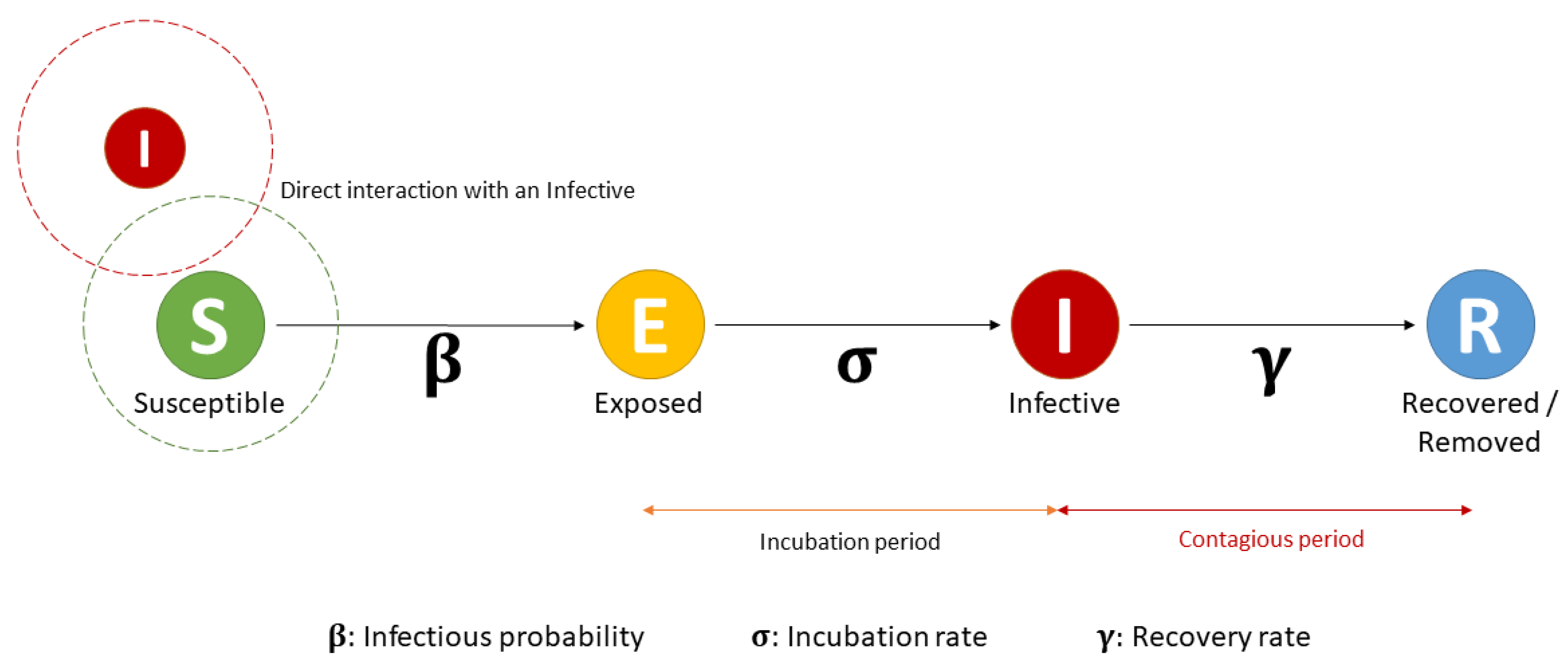
Epidemiologists have adopted different responses to epidemics and pandemics throughout history, depending on the knowledge, tools and skills developed at the time. Mathematical models of the spread of infectious diseases were first published by Kermack and McKendrick in 1927 [6]. These mathematical models are simplifications of reality that use differential equations to explain the evolution of a disease in time. An example is the SIR model (ibid), that divides the population in three different categories (‘Susceptible’ (S), ‘Infective’ (I) and ‘Recovered’ (R)) [6]. A probability value () identifies the likelihood that a ‘Susceptible’ person can be infected when in close contact with an ‘Infected’ person: and a recovery rate parameter (), which is the inverse of the infectious period, quantifies the duration of the disease in the ‘Infective’ person. Thus, the following system of ordinary differential equations (Equations (1)–(3)) defines the evolution of the disease in time between categories based on the parameters [6]:
Technological development has recently allowed agent-based models (ABMs) to become a useful tool in epidemiology. ABMs are stochastic computer simulations of simulated individuals (agents) in space and time [7]. Agents move and interact autonomously in the environment following a set of defined rules and based on their individual characteristics [8]. ABMs are particularly appropriate when agents’ behaviours are a complex function of agent attributes and characteristics, environments, and inter-agent interaction over time, being particularly well-suited for research that is concerned with understanding social processes [7]. Though the system is modelled from the individual point of view, its main properties are visualised and analysed from a global perspective, observing emergent complexity [9]. Another important factor is that ABMs are easily customised to study other similar scenarios by simply adjusting the modelled timeline and parameters that define the new scenario [10].
The combination of agents’ interactions in space and time with a mathematical epidemic model (e.g., SIR) representing the evolution of an infectious disease provides an alternative approach to simulate the spread of a disease in society from an individual (agent) perspective. One of the most interesting aspects ABMs contribute to epidemiology is that spatial and temporal factors are considered in the transmission of the disease. The use of ABMs pursues the progression of a disease and tracks the contacts of each individual with others in the relevant social networks and geographical areas [10].
Willem et al., 2017 [11] reviewed epidemiological investigations using ABMs and found that most studies were related to unspecified close-contact diseases (mostly used to describe methodology and transmission dynamics), closely followed by influenza, where many papers were published shortly after the 2009 H1N1 pandemic and the Ebola outbreak in 2015. They also observed a shift in the use of ABMs from methodological (43% to 19%) to application and intervention-related purposes (21% to 44%).
New epidemic ABMs have been developed recently due to the current COVID-19 pandemic. Masoud Jalayer and Orsenigo 2020 [12] developed an ABM (CoV-ABM) to simulate spatiotemporal COVID-19 outbreaks at any geographical scale (ranging from a village to a country) and one-hour timestamp, using census data of people and GIS information to simulate their routines and interactions in different geographical locations. The mathematical epidemic model applied was SEIHRD (Susceptible, Exposed, Infective, Hospitalised, Recovered, Dead). The model was applied in the State of Delaware, United States, simulating scenarios of no restrictions and quarantine only, where the top three infection locations were schools, houses, and universities when no restrictions were imposed, but in the quarantine scenario these changed to hospitals, public transportation and houses [12].
The ‘INFEKTA’ ABM [13] analysed the transmission of the infectious disease in the city of Bogotá (Colombia) with a one-hour timestamp. A modified SEIR (Susceptible, Exposed, Infective, Recovered, see Section 2.3) epidemic model (SEIRMID) was applied, and medical preconditions, age and daily routines were considered for each agent. Different scenarios applying only social distancing rules were simulated, showing that it is possible to establish a medium (i.e., close to 40% of the places) social distancing policy to achieve a significant reduction in the disease transmission.
Cuevas 2020 [9] developed an ABM to evaluate the COVID-19 transmission risks inside facilities only, simulating the spatiotemporal transmission process. The probability of a person being infected depends on several factors that range from health conditions to their discipline in following prevention measures.
Silva et al., 2020 [14] developed ‘COVID-ABS’, an open software SEIR agent-based model of COVID-19 epidemic that simulates health and economic effects of social distancing interventions in a one-hour timestamp but not considering the geospatial environment of any specific area of the world as some of the previous cited projects. Seven different scenarios of social distancing interventions were analysed (do nothing; lockdown; conditional lockdown; vertical isolation; partial isolation; use of face masks; and use of face masks together with 50% of adhesion to social isolation). The simulations support the notion that lockdown and conditional lockdown were the best scenarios in terms of controlling the number of infected and deaths.
Shamil et al., 2020 [15] proposed an agent-based model that simulates the spread of COVID-19 among the inhabitants of a city with a one-hour timestamp, considering five possible states in agents (healthy, infected noncontagious, infected contagious asymptomatic, infected contagious symptomatic and recovered). This analysis was developed and validated in Ford County, KS (USA), using demographic data related to the inhabitants, data related to the COVID-19 disease and physiological characteristics. The study showed that lockdown regulations alone can result in fewer people being infected in total compared to contact tracing approaches, and combining lockdown and contact tracing surpasses all the other interventions significantly.
Hoertel et al., 2020 [16] developed an open-source stochastic agent-based microsimulation model of the COVID-19 epidemic in France, simulating lockdown and post-lockdown measures, including physical distancing, mask-wearing and shielding of the population at risk of severe COVID-19 infection. Results showed that while lockdown is highly effective in containing viral spread, it would be unlikely to prevent a rebound and the need for a second lockdown, regardless of duration of the lockdown period.
These previous studies demonstrate that ABMs are an effective tool for simulating the transmission of COVID-19 and assessing the effectiveness of measures taken to reduce infection. Some research gaps remain, however:
(1) Previous research projects are focus on the whole population of a country ([12,16]), city ([12,13,15]) or not applied to any specific geospatial area of the world ([9,14]). Analysis of a more concise and specific group of the society in a well-defined and compact geospatial area could help to simulate how the disease is transmitted and to test the efficiency of the measures to reduce the risk within them with more a detail.
(2) Timestamp resolution in previous projects was one-hour (when data provided, e.g., [12,13,14,15]), which indicates many of the social interactions’ agents have are not considered during their daily routines.
(3) Only one of the previous cited research projects [16] developed a case-study where several measures to reduce transmission were simulated and compared, but the geospatial area of a real city was not considered. Simulation of different case scenarios in a defined urban area, considering the real location of buildings, roads and realistic agents’ daily routines, could combine these factors.
In this paper, we present a new agent-based simulation model to explore, from a geospatial perspective, the transmission of COVID-19 in a one-minute timestamp between students living in university accommodation and potential measures to reduce their risk of infection. The model was developed to simulate a case study based on Newcastle University in the UK. Five case scenarios (no measures, facemask use, lockdown, self-isolation and, a combination of measures) were simulated to identify their effectiveness at reducing the number of exposed and infected students at the end of the outbreak, the length of the virus in the environment, and the locations of high transmission.
This paper is organized as follows: Section 2 explains the methodology followed to develop the 3D ABM using GIS data and an epidemic model (SEIR) to simulate the presence of COVID-19 in the environment, and the development of the scenarios to reduce the risk of transmission. Section 3 shows the results and interpretation of each of the scenarios from a geospatial perspective, highlighting the most relevant findings from each. Section 4 discusses the findings and concludes with a summary of limitations in the study future work.
2. Materials and Methods
A methodology was developed to implement an ABM for the study of a COVID-19 outbreak amongst university students, building on the literature reviewed above. The methodology uses open-source software, ensuring wide uptake, and widely-available spatial data. This section will describe the ABM platform selected for use, the input data required for the study, the code development, the generated output data, the development of COVID-19 scenarios, and the assumptions and limitations found in the model.
2.1. ABM Platform Selection
There are many free and open-source ABM platforms that can be used to develop an epidemic simulation (e.g., [17,18,19]). The selected platform for this project was GAMA, a modelling and simulation development environment for building spatially-explicit agent-based simulations [18] that can be applied to urban areas (e.g., road traffic [20]), epidemiology (e.g., flu outbreak [21]) and the combination of both (e.g., disease spreading in a small city [22]). It was selected due to its easy and interpretable code language (GAML: GAma Modeling Language), its rich online documentation with quantitative and qualitative tutorials and its large variety of input and output formats. Appendix A shows a comparison of various open-access ABM platforms considered for this project.
2.2. Input Data
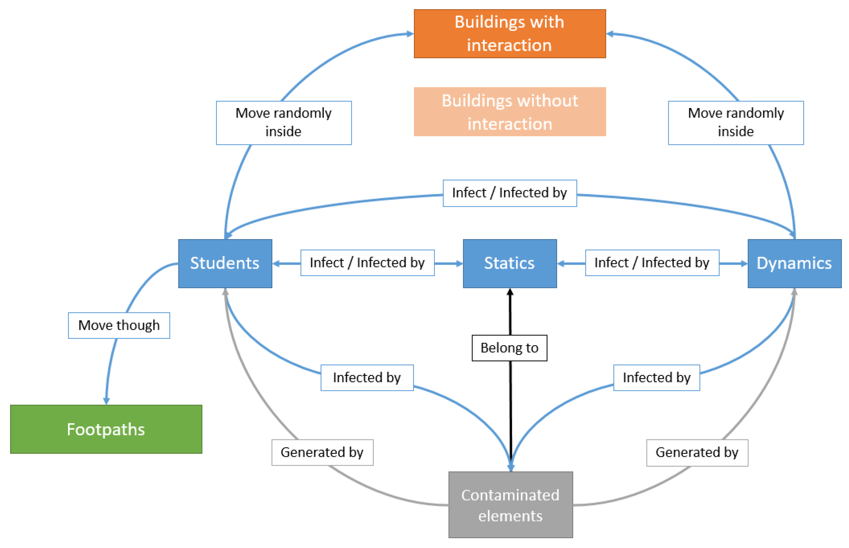
GAMA allows the use of geospatial data to represent the agents that interact in space and time within the model, with specific behaviours depending on their nature and characteristics. Five agent types were required in this project: buildings, footpaths, students, dynamics and statics.
2.2.1. Buildings
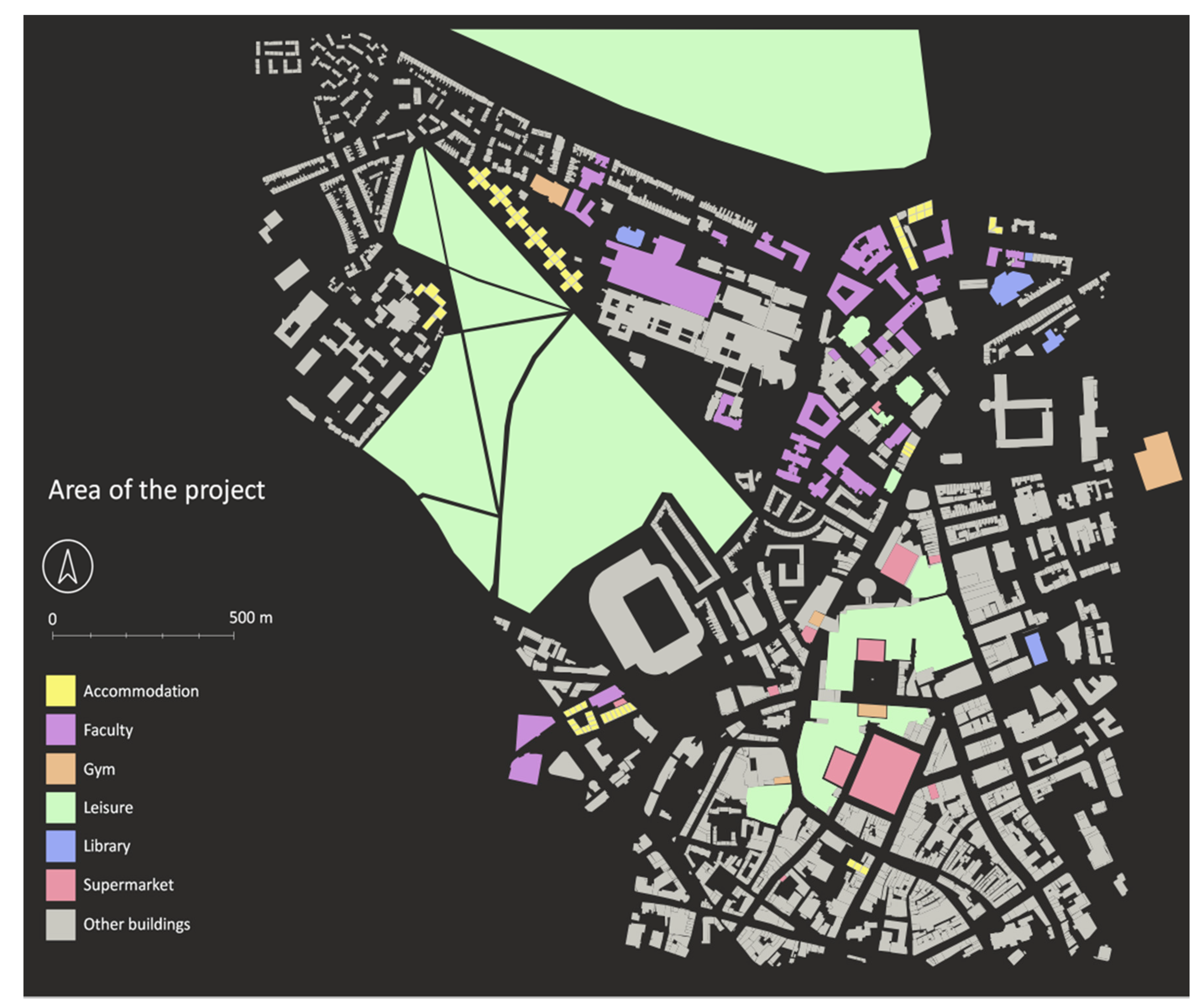
Buildings are 2D polygons that represent the location of each activity area in the study region of the model. OS Mastermap building data were obtained from the Digimap website [23] with ‘Building Height’ attribute [24] employed to obtain the ground level and base of the roof for each building. These two attributes allow the estimation of building height and approximate number of floors (assuming each floor is 4 m high). After the number of floors were calculated and stored as an attribute, polygons were manually classified into different types (i.e., ‘Accommodation’, ‘Faculty’, ‘Library’, ‘Gym’, ‘Supermarket’, ‘Leisure’ and ‘Other’), depending on their nature (2481 building features were considered in the area of study). ‘Other’ buildings are included for context but do not have any interaction with other agents in the model (2342 ‘Other’ features in total). Figure 1 shows the area of the project and the range of buildings included.
Each building type was assigned a speed attribute value that indicates the pace student and dynamic agents (see Section 2.2.5) move when within them (Table 1). These speed values were estimated by the authors to reflect the type of interactions and activities expected in each building.
Finally, ‘Accommodation’ buildings were divided in sub-units in order to simulate different apartments per floor. This avoids the spread of the disease between students that rarely have contact in real life. These sub-divisions were done based on the average number of students that share apartments in each student accommodation, according to a summary of accommodation provided by Newcastle University [25].
2.2.2. Footpaths
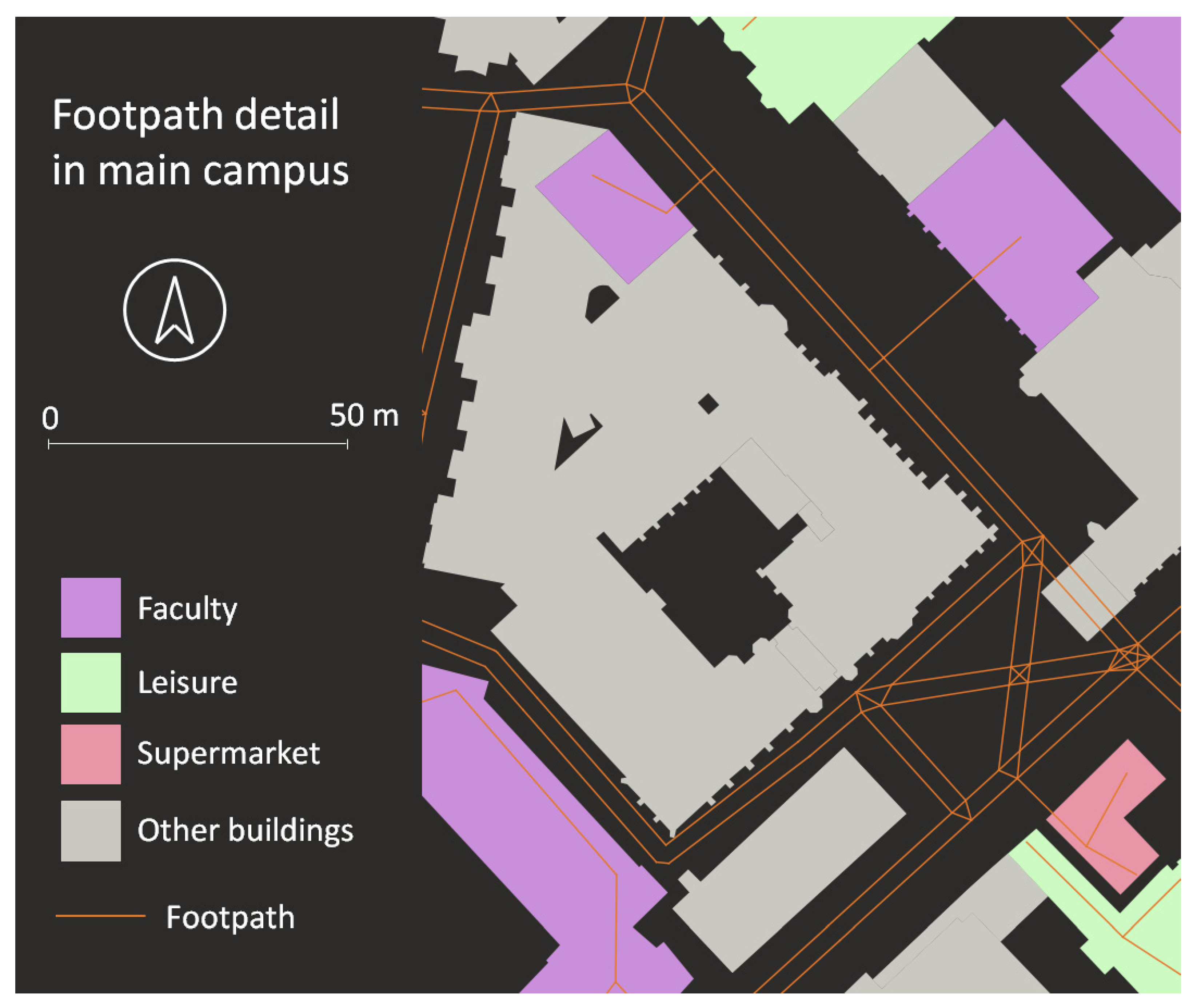
Footpaths are 2D line features representing the routes students use to go between buildings in their daily routines. These data were generated using Ordnance Survey ‘OS OpenMap Local roads’ layer [26]. This layer was used to create parallel footpaths 1.5 m apart using QGIS software. Since the GAMA platform calculates shortest path routes for agents, two tracks per street were created to allow sufficient realistic interactions between students outdoors (3426 ‘Footpath’ features were used in total). A detailed view of the generated footpaths can be observed in Figure 2.
Additionally, the entrance and main corridors inside buildings were digitised to ensure student agents share the same entrance (Figure 2). Manual connections were digitised in the intersections between the footpaths and all line strings were exploded to guarantee they are single lines as required by GAMA.
2.2.3. Students
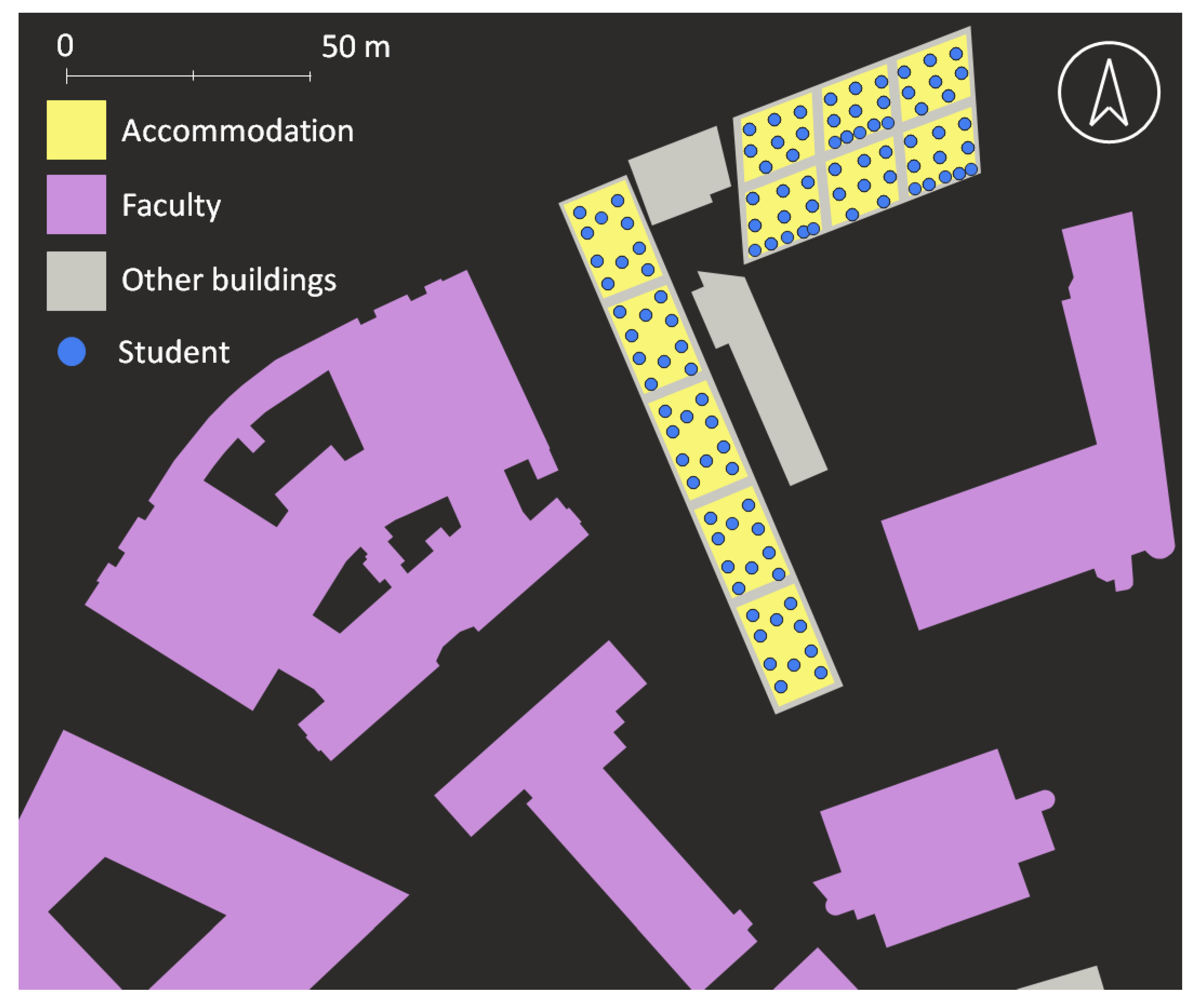
Student agents represent students attending Newcastle University and living in university accommodation [25]. In 2020, 10 residences were offered to undergraduates and 6 to postgraduates. In order to keep only accommodation with similar characteristics, accommodation with a maximum of one student per room, a range of 6–10 students sharing kitchens, and within walking distance of the main campus was selected. This gave nine accommodation locations with a total of 2954 student. These students were generated as 2D geometry points, located inside the sub-building divisions created previously in the accommodation buildings and at different floors (integer value in the attribute table, depending on each building’s number of floors), keeping the range of students per apartment as shown in Table 2. Agents were initialised with a 2 m minimum distance between them, representing the personal space each student has in order to avoid transmission of the disease during the night when everyone is sleeping. Figure 3 shows a detail of initialised students in the accommodation.
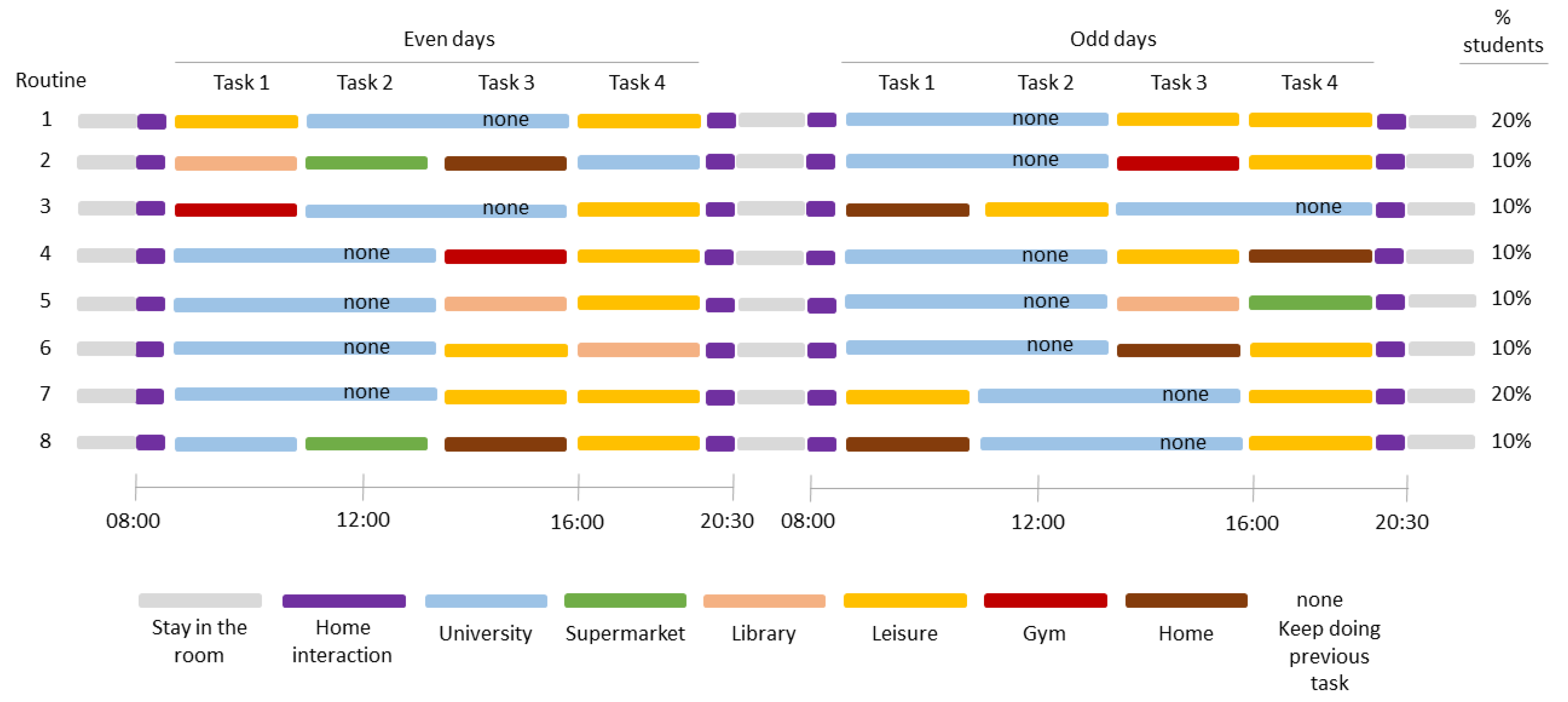
Each student was then attributed with daily routines, which consist of four tasks undertaken by each student during the day for a specific period of time (once outside of the accommodation). These tasks are shown in Table 3:
Eight different daily routines (differentiating between even and odd days) were created for students based on these tasks. The percentages of students assigned to each routine were decided assuming everyone attends a faculty building every day, 30% of students go to a gym, 30% go to the library, 70% enjoy leisure time and 30% go to supermarkets. These percentages were assigned arbitrarily based on assumptions. Figure 4 summarises the eight different daily routines created:
Students were randomly selected, assigned to one of these routines and linked to a specific building related to each task. These routines and locations were then stored along with the initial times for each task in the attribute table. This procedure was undertaken based on the following criteria:
- Each student was linked to a unique faculty building randomly. The number of students per faculty building were obtained from Newcastle University’s Press Office [27], where distribution of students by faculty (academic year 2019–20) is provided. These values were then spread in the different buildings each faculty has based on the area of the building (floor area × number of floors), assuming large buildings receive more students than small ones.
- Students attending gyms were assigned to a unique gym. The number of students per gym were calculated based on the data provided by Newcastle University Sport Centre and then extrapolating them to other gyms based on the size of the buildings. Approximately 50% of students were linked to the closest gym from their accommodation. The remaining were linked randomly to another gym.
- Students visiting libraries were linked to a unique library building. The procedure of assigning students to each building was similar to the one followed before for gyms, based on the size of the building. Approximately 50% of the students were assigned to the closest library, while the rest were assigned to another, randomly.
- Students shopping at supermarkets were linked to a unique supermarket too. In this case, 50% of the students were assigned to the closest supermarkets to campus and the other 50% to another supermarket based on the size of the building. It was assumed students do their shopping close to their accommodation in order to carry their belongings the shortest time as possible.
- Leisure areas are parks, shops, and university buildings where students relax or get advice. Students were linked to one leisure area for each task related to leisure time, assuming no one goes to a park early in the morning but many during the evening and the opposite for university buildings. Students were spread randomly in these areas based on their size, not on proximity as in previous tasks.
2.2.4. Static Agents
Static agents refer to any unanimated element in the environment that can transmit an infectious disease when has been in close contact with an ‘Infective’ agent. Examples are door handles, items in the toilet, computers in labs, and items in supermarkets. These agents were located inside buildings based on assumed probability of interaction, the likelihood to be infected when in contact, and the approximate number of times students interact with them, in each type of building. Table 4 shows the proportion of Static agents included in each building type per unit area (e.g., gyms have four times more static agents than accommodation, library and leisure buildings). Based on these values and the size of each building, there were spread 477 static agents inside the buildings.
2.2.5. Dynamic Agents
Dynamic agents refer to any person that can interact with students in their daily routines and static agents. They can be considered as other students, professors, university staff and customers in supermarkets or stores, etc. A total of 471 dynamic agents were located inside buildings. These agents do not follow any daily routine and are always moving randomly inside the building they were located.
The number of static and dynamic agents was chosen based on available computing power and processing time of the model.
The attribute table of each described agent can be found in Appendix B.
2.3. GAMA Code Development
Based on GAMA tutorials [28], model code was developed to import geospatial data into the model, develop behaviours for each type of agent, and export output files. Additionally, the code was implemented and improved with new conditions and behaviours related to the purpose of the project, such as the existence of dynamic and static agents, the use of different speed values depending on the building’s type, and the use of a SEIR epidemiological model.
Several functions were created to simulate the movement of students in their daily routines. Students move in the environment based on their tasks and starting times allowing the simulation of the following activities:
- In the morning, between 08:00 and 08:30, they interact with other students moving randomly in the accommodation.
- Between 08:30 and 09:30, they start their first routine and go to their assigned location following the shortest path using the footpaths at a random speed between 3 and 5 km/h.
- For their first task inside a building, they move randomly at a speed based on the type of building, until time to start next task is triggered and move to that place through the footpaths again.
- Once their last task is finished, they go back to the accommodation, where they interact randomly with their flatmates until 20:15–20:30, when they go to their initial location, symbolising their own room with at least 2 m distance to any other student.
- They remain there until the next day, when their interactions start again with their flatmates at 08:00.
Dynamic agents only move randomly inside buildings (always in the same floor level) at a speed specified by the building’s type, while static agents do not move and are always located in the same position.
Once movements of the agents were created based on space (buildings and footpaths) and time (initial time to start the tasks), an epidemiological SEIR model was introduced for students and dynamics. The SEIR epidemiological model is an extension of the SIR model described in Section 1, including an intermediate ‘Exposed’ (E) category that describes individuals infected but not infectious (Figure 5).
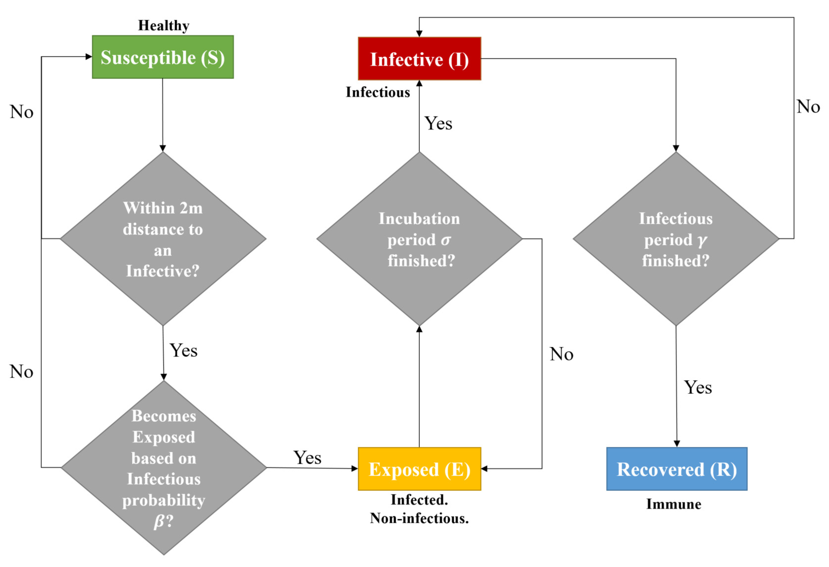
Based on GAML code developed by Benoit Gaudou [29] and Tri and Hqnghi [30], this SEIR model classifies the agents as ‘Susceptible’, ‘Exposed’, ‘Infective’ and ‘Recovered’, depending on their status related to the infectious disease (Figure 5). The model divides agents in these four categories and transitions between them are based on three parameters (probability to be infected (β) when in close contact (within 2 m distance) with an infectious agent; the incubation period (σ); and the recovery period (γ)). Additionally, β value was split in two options, depending if agents are located indoor or outdoor. It was considered that probability to be infected indoor is more likely than outdoor because outdoor there is a large volume of clean and fresh air, making transmission more difficult but not impossible [31]. This condition was implemented in the code, assigning a greater β value when students are indoor than outdoor (these values are set up by the user before running the simulations). When a ‘Susceptible’ agent (student or dynamic) is within 2 m distance (3D distance) of an ‘Infective’ (student, dynamic or static) agent, and based on β value (indoor or outdoor), the ‘Susceptible’ agent can be converted into ‘Exposed’ (infective but not contagious) or remain ‘Susceptible’. If it is ‘Exposed’, then it becomes ‘Infective’ to others after σ days, and ‘Recovered’ after γ. A flow diagram representing the evolution of agents can be observed in Figure 6.
These functions were created in GAML by selecting the ‘Susceptible’ agents within 2 m distance of an ‘Infectious’ agent and then calculating the probability value to infect them. Functions to convert agents into ‘Infective’ and ‘Recovered’ were based on time (σ and γ values) only.
Studies have observed that the COVID-19 virus can be active on surfaces for a time [32], with experiments showing that SARS-CoV-2 and SARS-CoV-1 can remain viable and infectious in aerosols for hours and on surfaces up to days. In the case of SARS-CoV-2, a viable virus was detected for up to 72 h on plastic and stainless steel although the virus was greatly reduced, while no viable SARS-CoV-2 was measured after 4 h on copper or after 24 h on cardboard [32]. Similar results were obtained for SARS-CoV-1. Since static agents, as unanimated elements, cannot follow a SEIR model (they do not have ‘Exposed’ status), they were classified in a SIS (Susceptible, Infective, Susceptible) model. Once a Static agent is infected by any other agent (in the same conditions as students and dynamics) it becomes ‘Infective’ and can infect others. If this ‘Infective’ static agent encounters a ‘Susceptible’ student or dynamic agent, these agents are infected with their probability value and the static agent again becomes ‘Susceptible’, being possible to be ‘Infective’ again. Based on [32], a variable ‘Infected’ lifetime for static agents was defined as a random value between 0 and 1439 (minutes in a day). When the assigned value is equal to the current minute of the day, then the ‘Infective’ static agent becomes ‘Susceptible’ again.
Finally, a new static agent was developed called a ‘Contaminated Element’, which represents any element that an ‘Infective’ agent (student or dynamic) can reproduce through coughing, sneezing, or touching, allowing the disease can be transmitted to others when in contact with those elements. Since COVID-19 can be transmitted by airborne particles, these ‘Contaminated Elements’ could represent particles in the air with the capacity to infect others in a short period of time. These ‘Contaminated Elements’ are generated based on a probability value decided by the user. If they infect someone else, they disappear from the model or, if not, they disappear after the same lifetime as static agents. They follow an ID (Infective–Die) model.
Figure 7 summarises the behaviours and interactions between the different agents in the model, with blue boxes defining the agents that can transmit the infectious disease directly, and the grey box defining the ‘Contaminated Elements’ generated by student and dynamic agents. Orange boxes define the buildings included in the model, while the green box identifies the generated footpaths. Arrows describe the relationships between the different agents during the simulations.
The developed model contains six initial parameters to be specified by the user before running any simulations. These parameters depend on the nature of the infectious disease and can be adjusted according to the disease being simulated (Table 5):
Additionally, the speed of agents within buildings can be adjusted in the attribute table of the building dataset and speed of students in footpaths can be adjusted directly in the code, while routine tasks and initial times for each student can be modified in the student dataset.
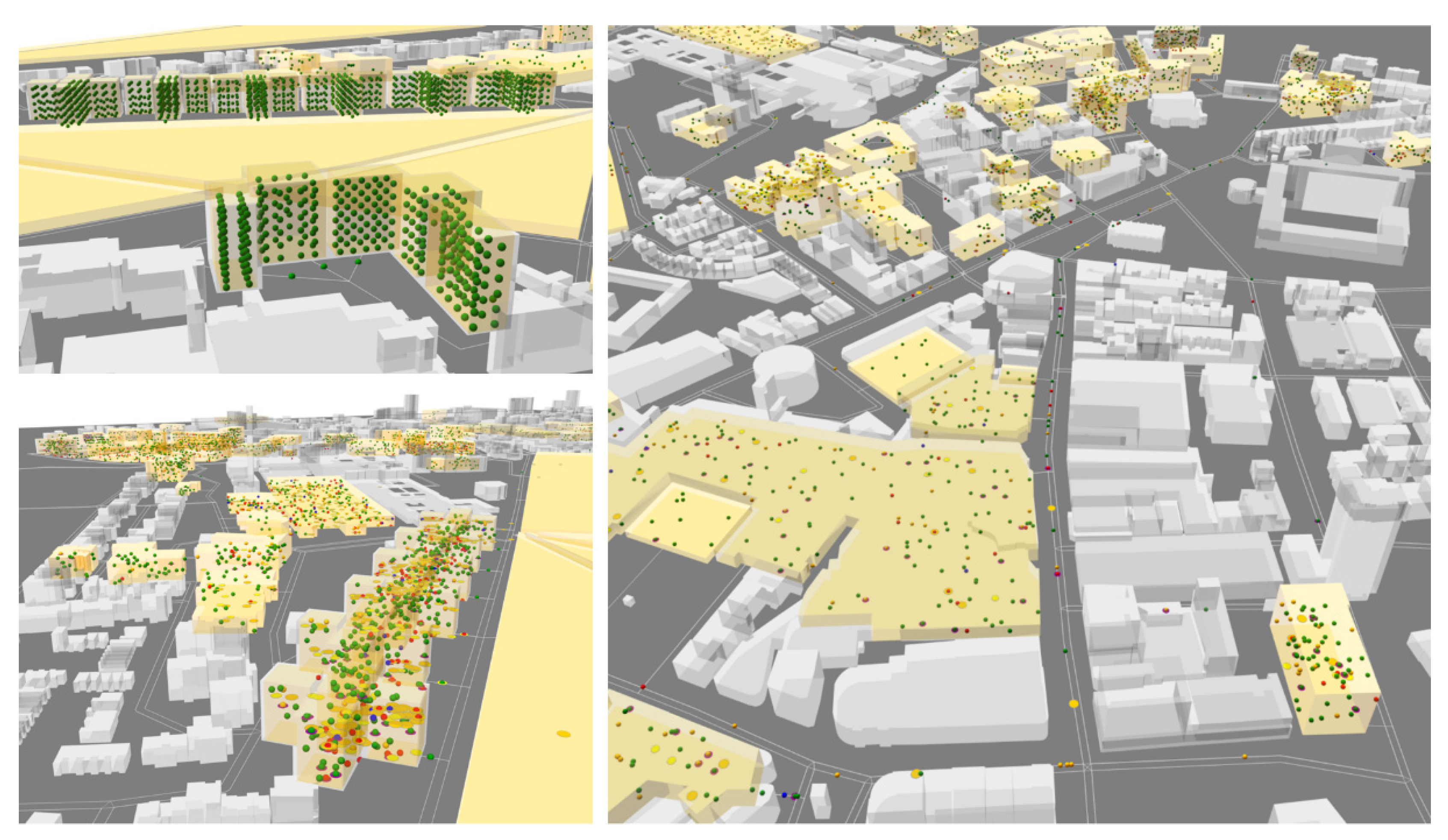
Figure 8 shows different perspectives of the 3D ABM developed showing agents (students, dynamics and statics) in different locations and in different colours depending on their infectious disease status (‘Susceptible’ (green), ‘Exposed’ (yellow), ‘Infective’ (red) and ‘Recovered’ (blue)):
2.4. Output Data
Simulations ended when the number of ‘Exposed’ and ‘Infective’ students reached zero, meaning the disease has disappeared from the environment. When these two conditions occur, four output files (three CSV and a text file) are generated, containing information about the evolution of the disease in space and time:
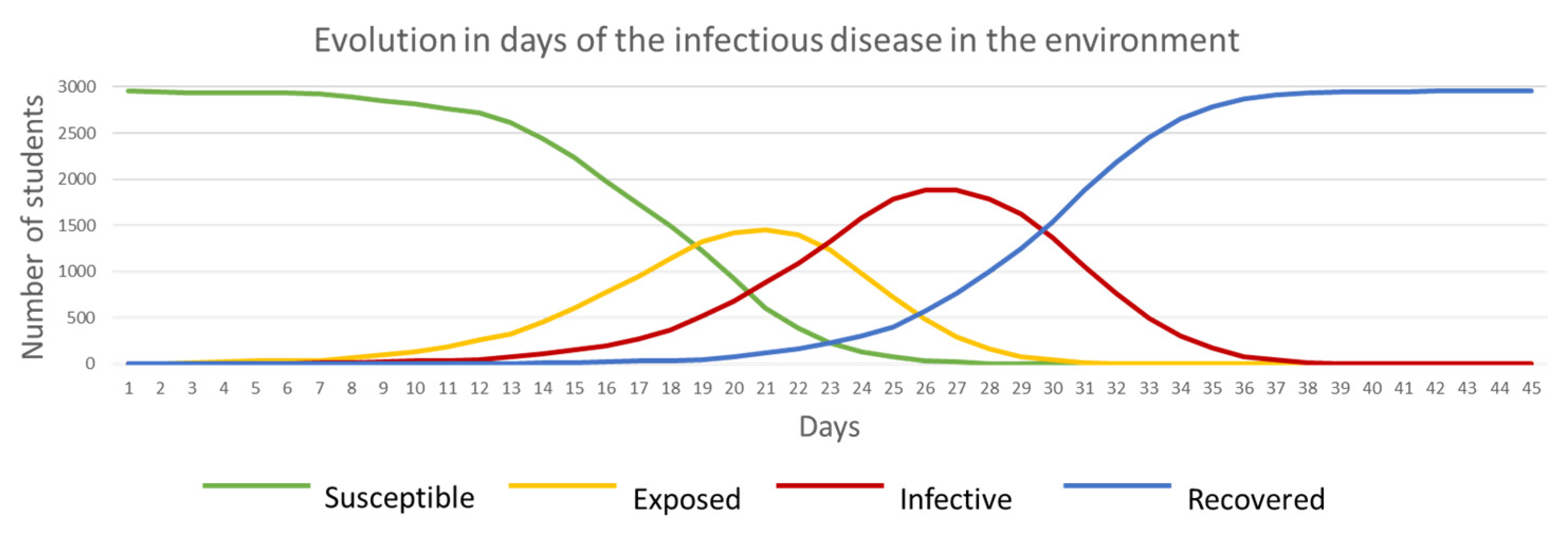
- ABM_SEIR_values_per_day.csv: this file contains the evolution in time of the disease. It shows the number of ‘Susceptible’, ‘Exposed’, ‘Infective’ and ‘Recovered’ students per day. When plotting this data in a chart, it is possible to identify the duration of the disease in the environment, when ‘Exposed’ and ‘Infective’ peak values were reached and the speed in the evolution based on the slopes of the curves (Figure 9).
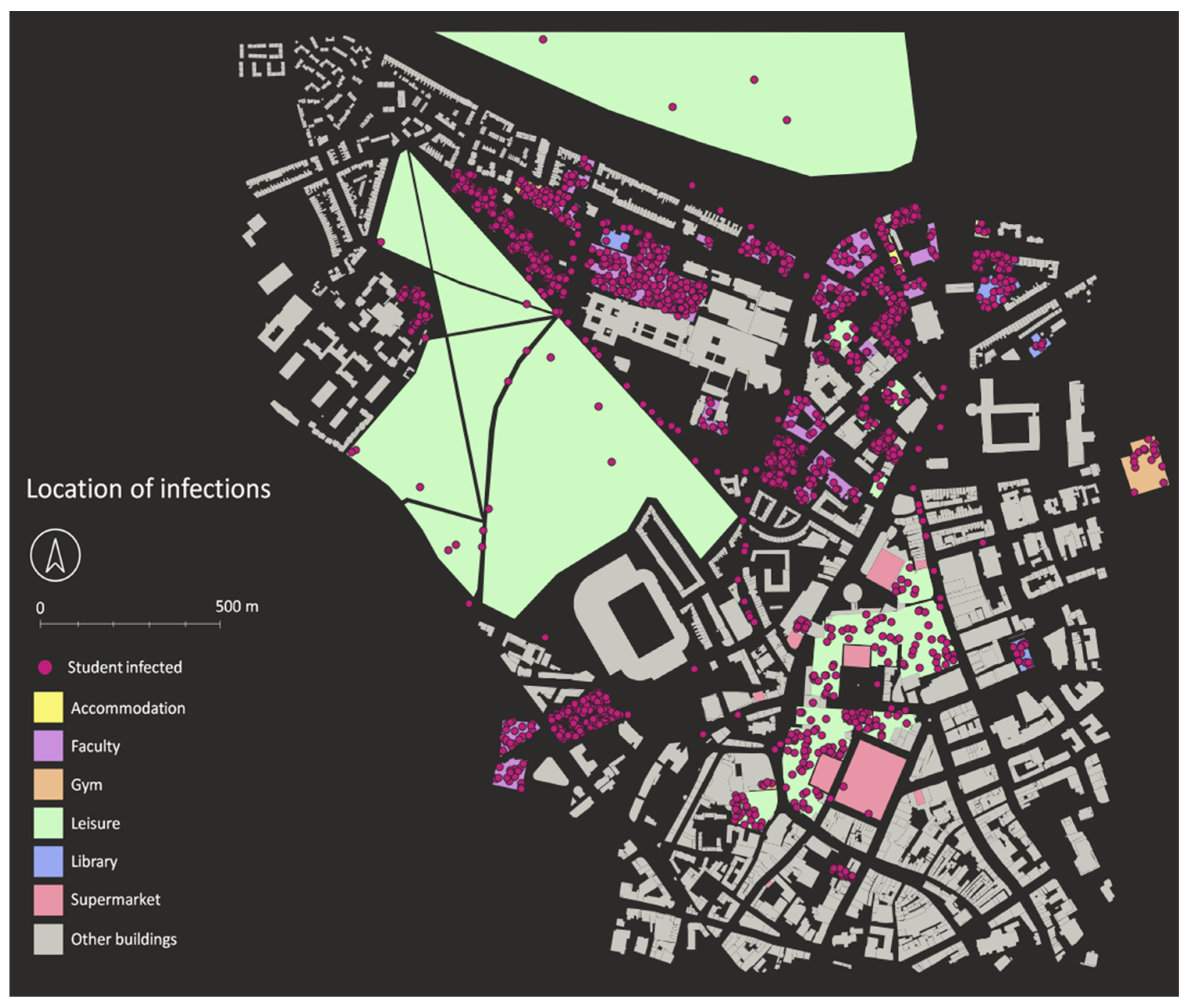
- Agents_after_simulations.csv: this file contains individual information of every student in the model, recording their status related to the disease (SEIR), and time and location (x, y, z coordinates in EPSG 27700) of infection and by whom in the case of infection. This information allows spatial analysis of infection, identifying the places where most infections occurred (Figure 10).
- Transmission_list.csv: this file contains information about how the disease was transmitted between agents recording the ID value and the ID value of the agent that infected them for each student, dynamic and static agent. This information allows tracking the transmission of the disease between agents and could be used to generate graph representations of transmission.
- Initial_data_and_parameters.txt: this file contains the initial input data and parameter values set up by the user before running the simulation. This file is useful to keep track of the parameters used in each simulation.
The attribute table of each described output file is shown in Appendix C.
2.5. Infectious Disease Scenario: COVID-19 Outbreak
As described above, the model has six initial parameters directly related to the infectious disease that need to be set up (Table 5). Some of these parameters can be obtained from literature, but due to the novel nature of this disease, there is some disagreement about accurate values. A reasonable consensus on σ and γ values was found in the literature, with WHO indicating the incubation period (σ) is between 5 and 6 days [33], while Public Health England indicates it is from 1 to 14 days (median 5 days) [2]. Five days was chosen for this value. The recovery period (γ) was set at 7 days based on Public Health England findings [34] (although this has since been modified to 10 days).
A greater variety of β (probability to be infected) values was found in the literature (Appendix D), however, suggesting that precise knowledge of the disease has not yet been achieved. In some cases, the value is given as time-dependent, and the range of values are not given. In others, the values ranged from 8.68 × 10⁻⁸ to 1.68, referred directly to the reproductive number of the area of study, or calculated values based on factors such as the location of the pandemic outbreak and the social interactions of the people in each area.
Since a definitive value could not be found, an approximate value for β indoor was determined related to the reproductive number (R0), which is the average number of secondary infections produced by an infectious case in a population where everyone is susceptible [35]. Four different scenarios were selected (each one run eight times) with different β indoor values (0.1, 0.05, 0.025 and 0.005) and constant σ and γ values (5 and 7, respectively). Then these simulations were analysed by calculating the average number of secondary direct (person-to-person) infections produced by students and dynamics using the ‘Transmission_list.csv’ file obtained from each simulation, obtaining the average and standard deviation results in Table 6. These average values cannot be considered as an equivalent to the R0 value because they were obtained considering all students during the simulation, while R0 definition estimates the value when everyone in the population is susceptible (i.e., at the beginning of the outbreak). For the purpose of this project, however, and given the difficulty obtaining a definitive β indoor value, a similarity between these infections and the R0 number was assumed.
These results were compared against the study by Flaxman et al. (2020) [36] where an approximate R0 for the UK was estimated between 3.5 and 4.0. Based on this R0 value, and assuming an excess value in the ones estimated in this project (‘Infected’ students and dynamics at the beginning of the epidemic should infect more people than others at the end of the epidemic), it was decided to use a β indoor value of 0.025 (R0 ≈ 3.10).
The rest of initial parameters related to COVID-19 infectious disease (β outdoor and probability to generate contaminated elements) were obtained based on β indoor, σ and γ values after several simulations. The number of ‘Infective’ people outdoors was decided to be minimum (approximately a 2% of all infections) and the approximate number of ‘Contaminated Elements’ generated by each ‘Infective’ person was one per infected day. All simulations commenced with two random initial ‘Infective’ students. Table 7 summarises the parameters selected to simulate a COVID-19 outbreak in Newcastle University:
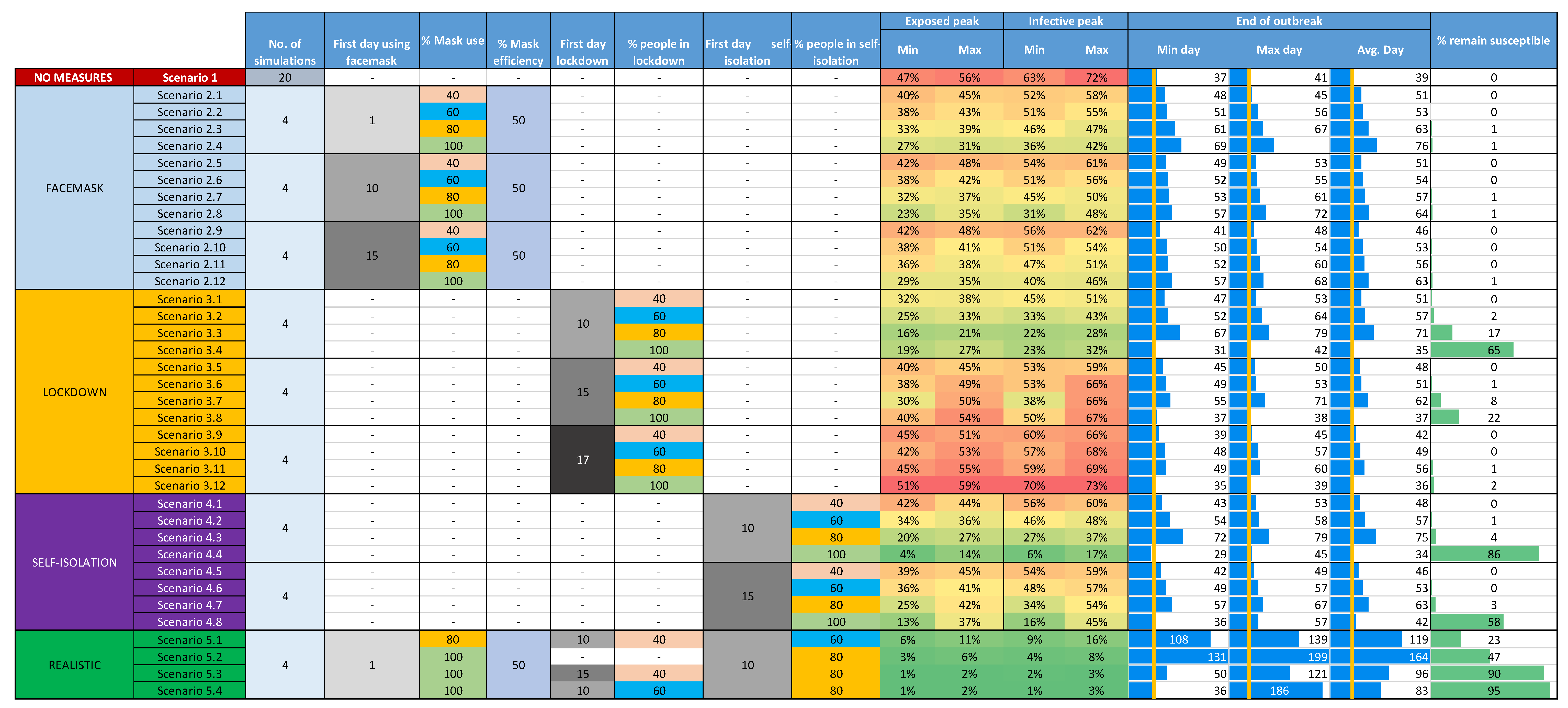
As ABMs are stochastic tools, where different results are obtained in every simulation, 20 simulations were run in order to identify the range of minimum, maximum and average values in the evolution of the disease in space and time.
A baseline scenario (Scenario 1: no measures implemented) was simulated, where the disease is only eradicated when ‘Susceptible’ agents reach 0, with ‘Recovered’ people being protected (‘herd immunity’); or the disease is weak and only infects a small proportion of the population.
2.6. Risk Reduction Measures
When an epidemic or pandemic occurs, measures to control and reduce the risk of the disease must be taken by the authorities, especially when pharmaceutical measures (e.g., vaccination) are not an option. Social distancing, for example, is a measure that reduces the risk by keeping a minimum distance between people, avoiding the transmission of the disease when in contact with ‘Infective’ persons. By avoiding contact, the infectious disease disappears after time.
Since COVID-19 is a very infective disease that requires measures to reduce transmission risk, a number of measures to reduce the risk of infection were analysed individually and in combination in the following scenarios:
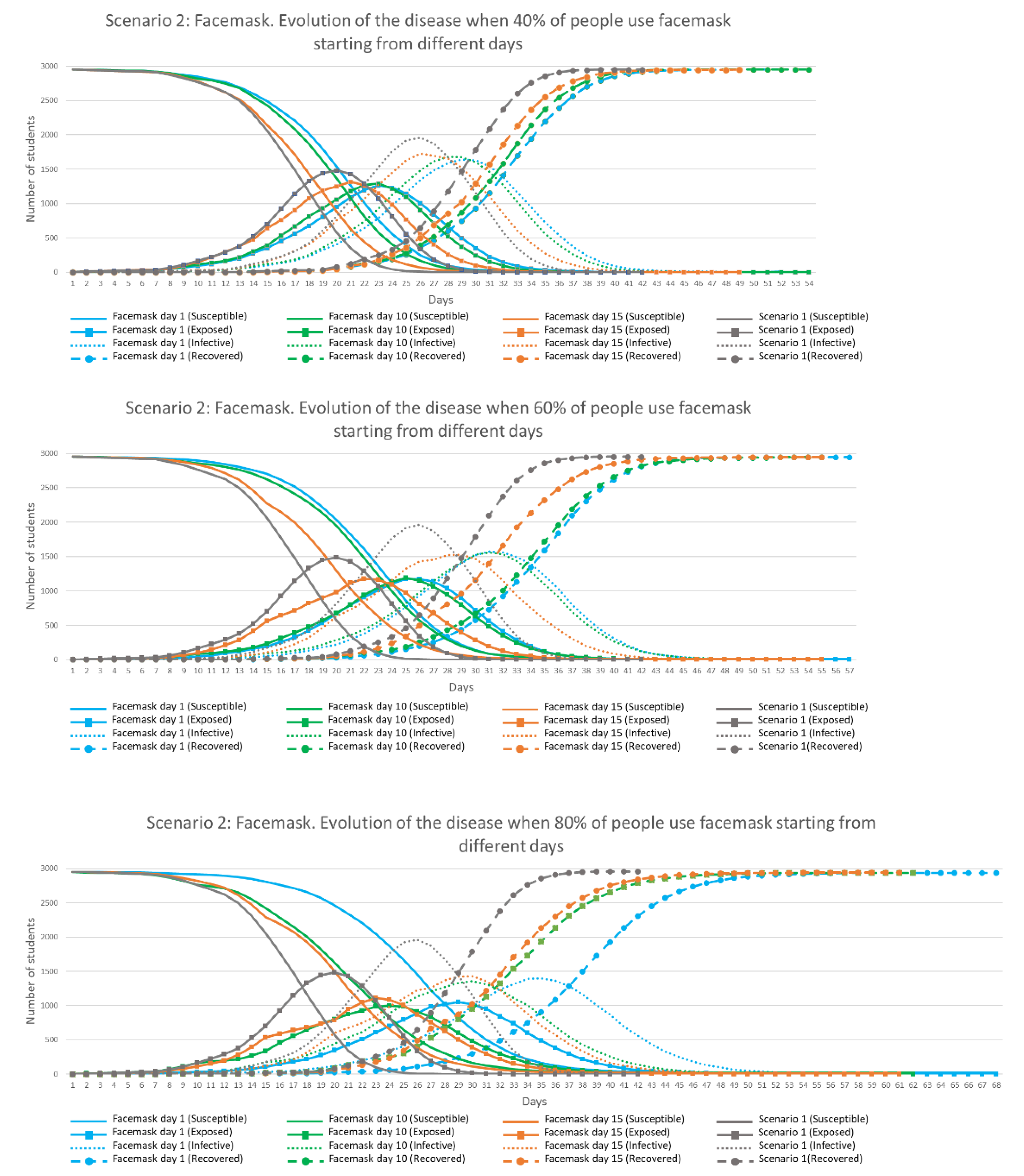
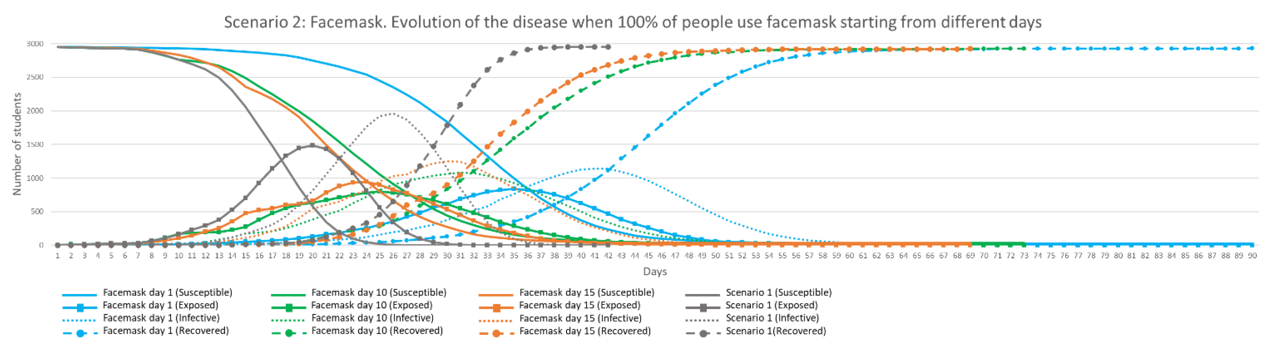
- Scenario 2: Facemasks: the use of facemasks to protect and reduce transmission is a controversial topic. WHO, in an Interim guidance from the 5 June 2020, highlighted a lack of evidence on the effectiveness of universal masking of healthy people in the community to prevent infection with respiratory viruses such as COVID-19 [37]. The guidance was updated, however, to advise that to prevent COVID-19 transmission effectively in areas of community transmission, governments should encourage the general public to wear masks in specific situations [37]. Some studies have shown that use of facemasks by the general public should be encouraged as soon as possible [38,39,40,41,42]. WHO additionally adds that the purpose of the use of face masks is two-fold, preventing transmission of the virus to others in case the wearer is infected (source control) and self-protection for a ‘Susceptible’ person (prevention) [37].
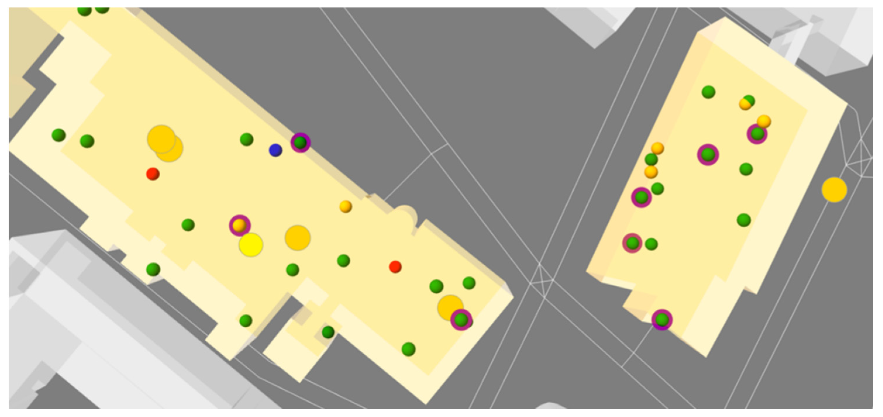
ABM simulations were developed for different proportions of student and dynamic agents using facemasks from different starting days. The percentage of people using facemasks were 40, 60, 80 and 100%, starting from Days 1, 10 and 15. A total of 12 simulations were run four times each in order to check the efficiency of each combination of options, with mask efficiency based on the literature [39] (20 to 80% efficiency for cloth masks, with 50% possibly more typical), set as 50% in all simulations. This indicates that when a ‘Susceptible’ agent wears a mask, the probability to be infected is reduced by 50% while when an ‘Infective’ agent wears a mask the probability to infect others and the probability to generate ‘Contaminated Elements’ is also reduced by 50%. These conditions were incorporated into the ABM code, identifying mask-wearing students and dynamics with a purple circle around them (Figure 11).
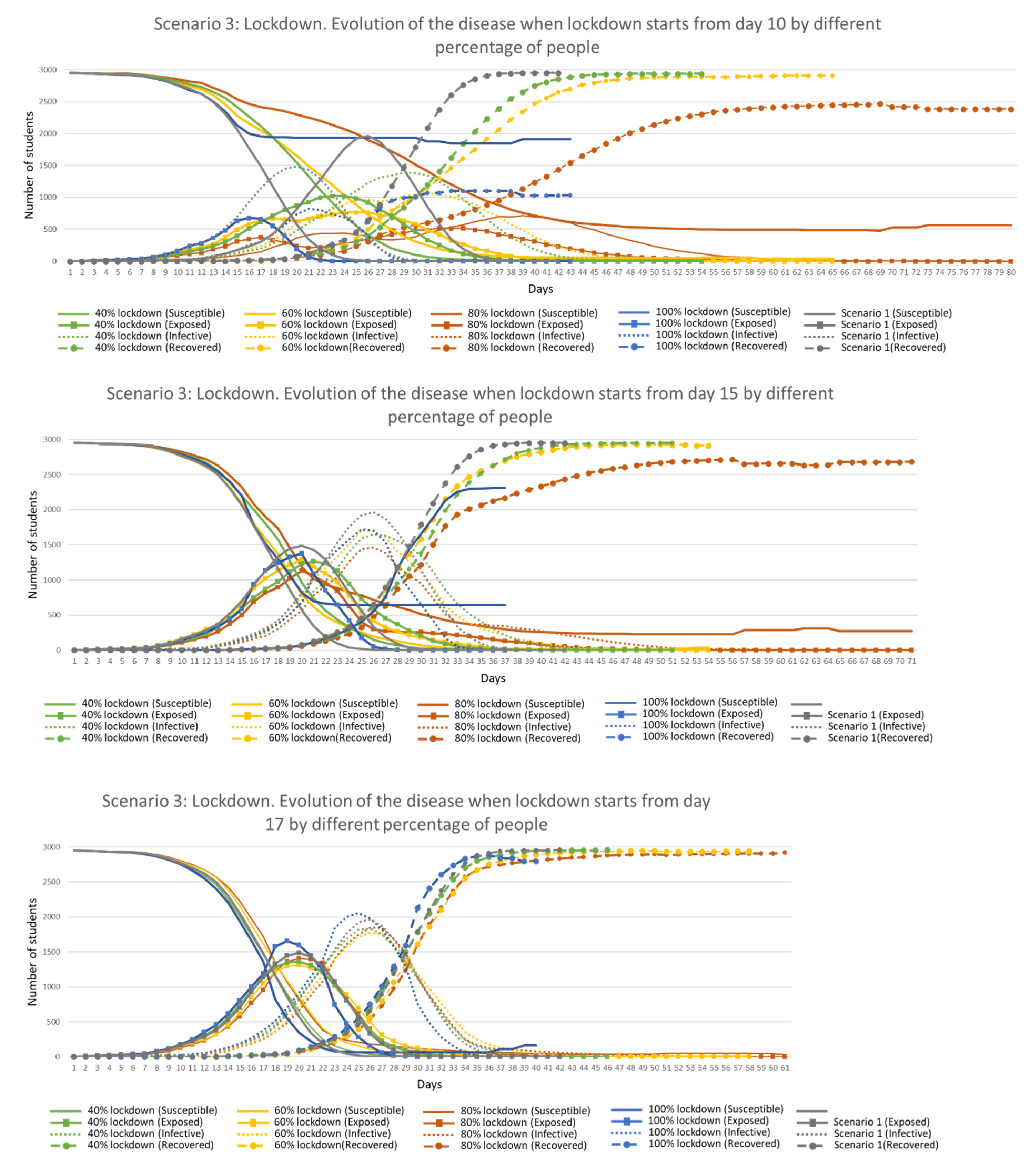
- Scenario 3: Lockdown: in a pandemic scenario, a ‘Lockdown’ consists of keeping people isolated at home to reduce the transmission of the disease. This is the most restrictive and extreme measure in terms of its impacts on the economy and personal freedom. In the UK, for example, GDP in April 2020 fell by 20.4% based on the negative impact of the national lockdown, the largest fall since monthly records began in 1997 [43]. This scenario was simulated in the ABM with a different percentage of randomly selected students kept at home (daily tasks were disabled for them) from a specific day during the epidemic. As in Scenario 2, the percentage of people in lockdown were 40, 60, 80 and 100%, starting from Days 10, 15 and 17 in this scenario. A total of 12 simulations of combinations of these values were run four times each to analyse their efficiency.
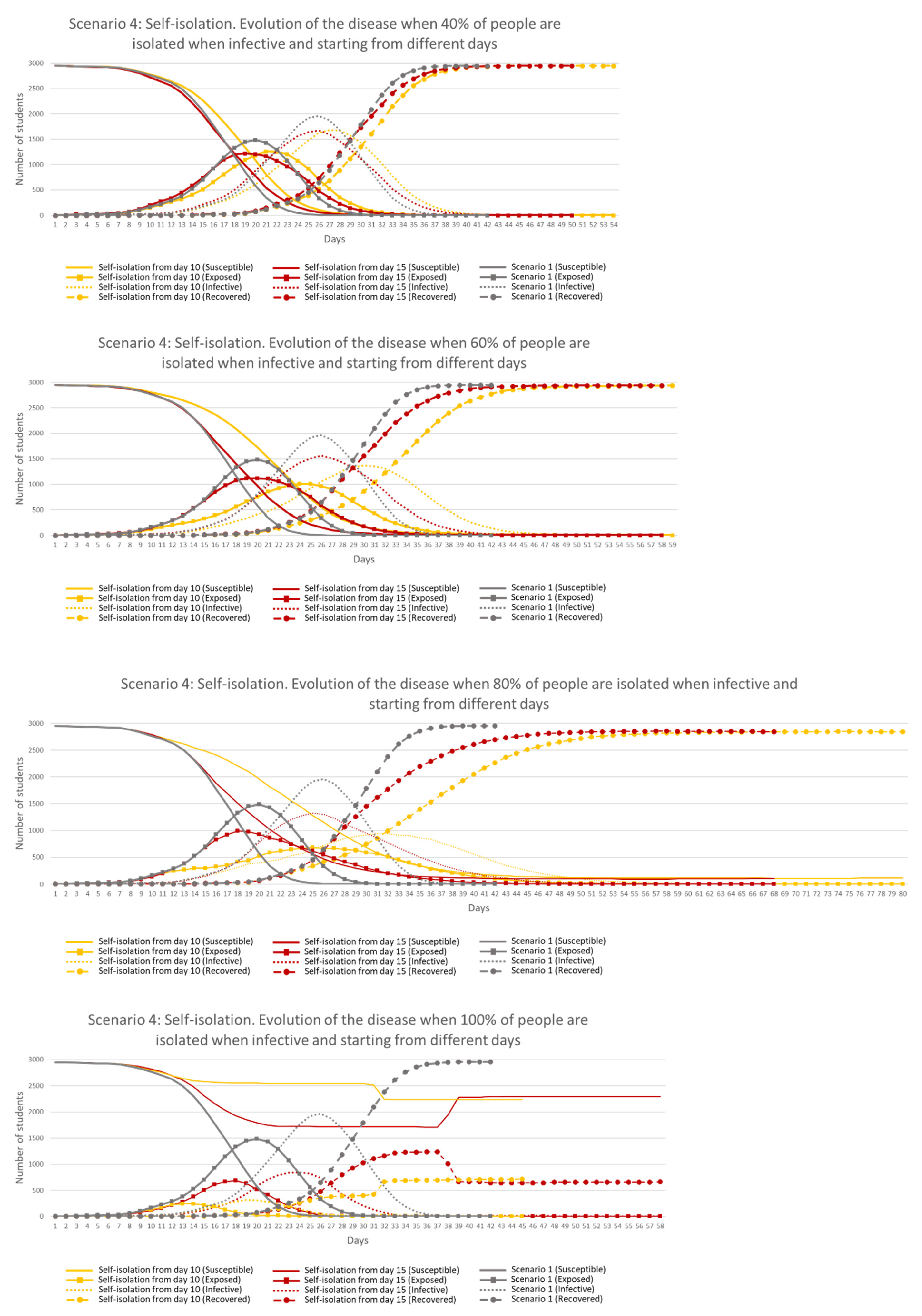
- Scenario 4: Self-isolation: self-isolation is a responsible act that an ‘Infective’ person does to protect others. For highly infectious diseases like COVID-19, ‘Infective’ people should stay at home away from others, however external factors, such as personal circumstances, work environment or lack of symptoms when ‘Infective’ (asymptomatic) influence this decision. This scenario was implemented in the ABM by either self-isolating an ‘Infective’ student or dynamic agent (assuming a test and trace contact) or allowing them to continue their daily routines based on a percentage value. If self-isolation is chosen, then the individual is moved to a safe location to avoid contact with flatmates. If self-isolation is ignored, the individual continues with their daily routines with the ability to infect others. Different percentages of adherence to self-isolation were simulated (40, 60, 80 and 100%), starting from Days 10 and 15 of the epidemic, with the parameters combined in eight simulations, each run four times to check their efficiency.
- Scenario 5: Realistic: in real life, these previous measures are not considered individually but in combination. Four simulations were run, four times each, combining some of the previous measures with different values in order to identify an optimum combination to remove the disease from the environment in a short period of time, with small consequences to the population, and keeping as many away from the disease as possible.
The decision about the selected days to apply these various measures was guided by the results obtained in Scenario 1. It was observed that in Day 10, 5% of the students were ‘Exposed’ and 1% ‘Infective’. In Day 15, the percentages were 25 and 5, while in Day 17, they were 31 and 10, respectively. Implementing measures at these times in the simulations allows the identification of the appropriate implementation time and testing when measures are not efficient because they were applied too late.
2.7. Model Simulation
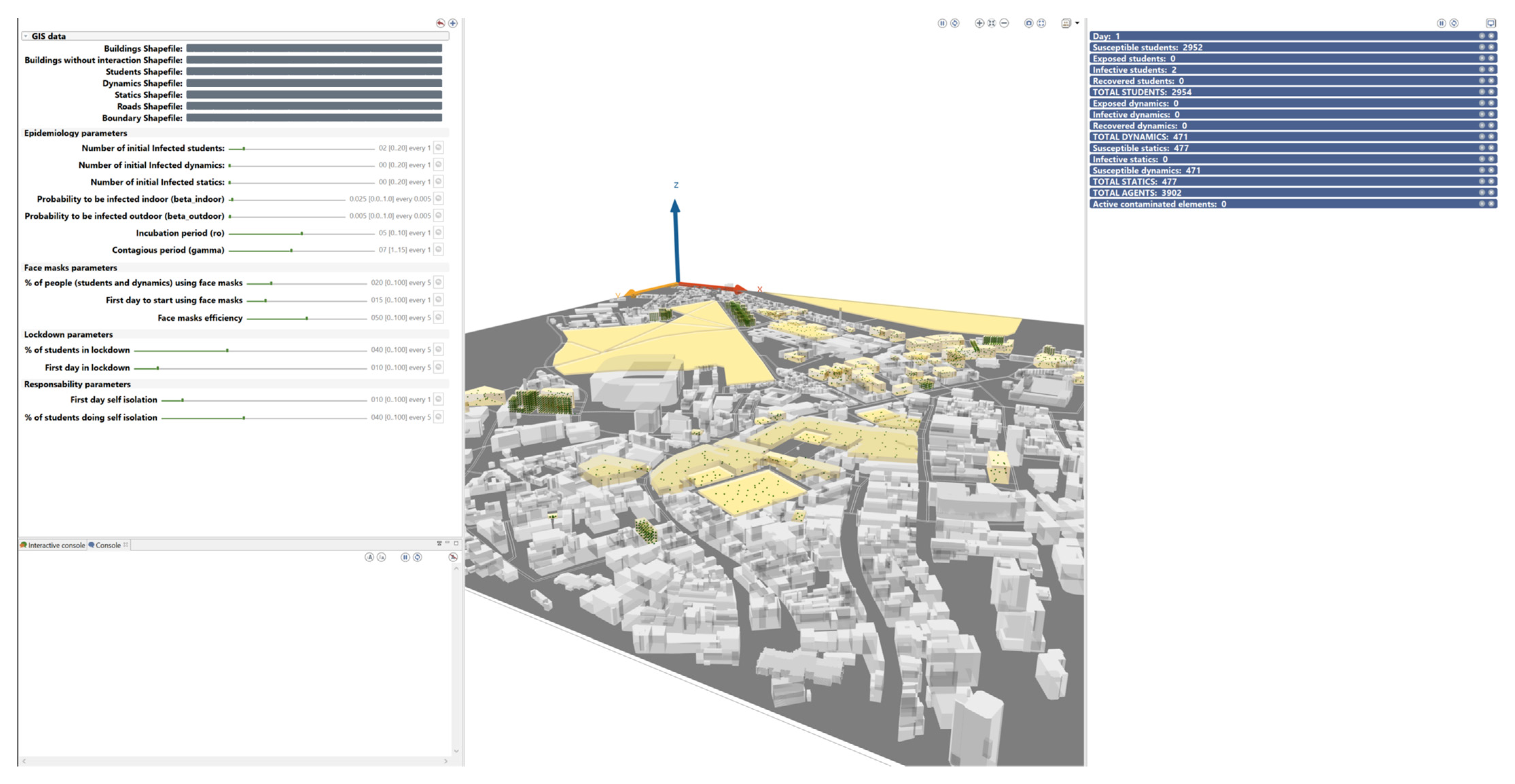
The model simulation can either be run using the graphic user interface (GUI), where the user can set up the initial parameters (left hand side of the interface), start the simulation and see how agents behave in real time (central part of the interface) and obtain real time information about the evolution of the infectious disease (right hand side of the interface). Figure 12 shows the GUI in the GAMA platform:
The model can also be run in batch mode, allowing several simulations to be run in parallel with the same parameters but with random starting conditions. Initial parameters are defined in the code and results are only shown when all simulations are finished.
2.8. Assumptions and Limitations
Simulations are run with one-minute time steps starting on the 14 March 2020. There is no differentiation of agents in terms of age or gender, and all accommodation is identical. All students return to their original accommodation each night. Students are assumed to be aged between 18 and 30 years, and as such deaths were not considered in the model as deaths from COVID-19 are almost zero in this age group [44].
Software requirements and characteristics of the laptop used in the research can be consulted in the Appendix E.
3. Results
The five scenarios described above were run and results obtained with different parameter values used to reduce the risk in the transmission of the disease. Results are interpreted from a spatial-temporal perspective with the aim of testing the efficiency of the measures to reduce the risk of COVID-19 transmission between the students.
3.1. Scenario 1: No Measures Implemented
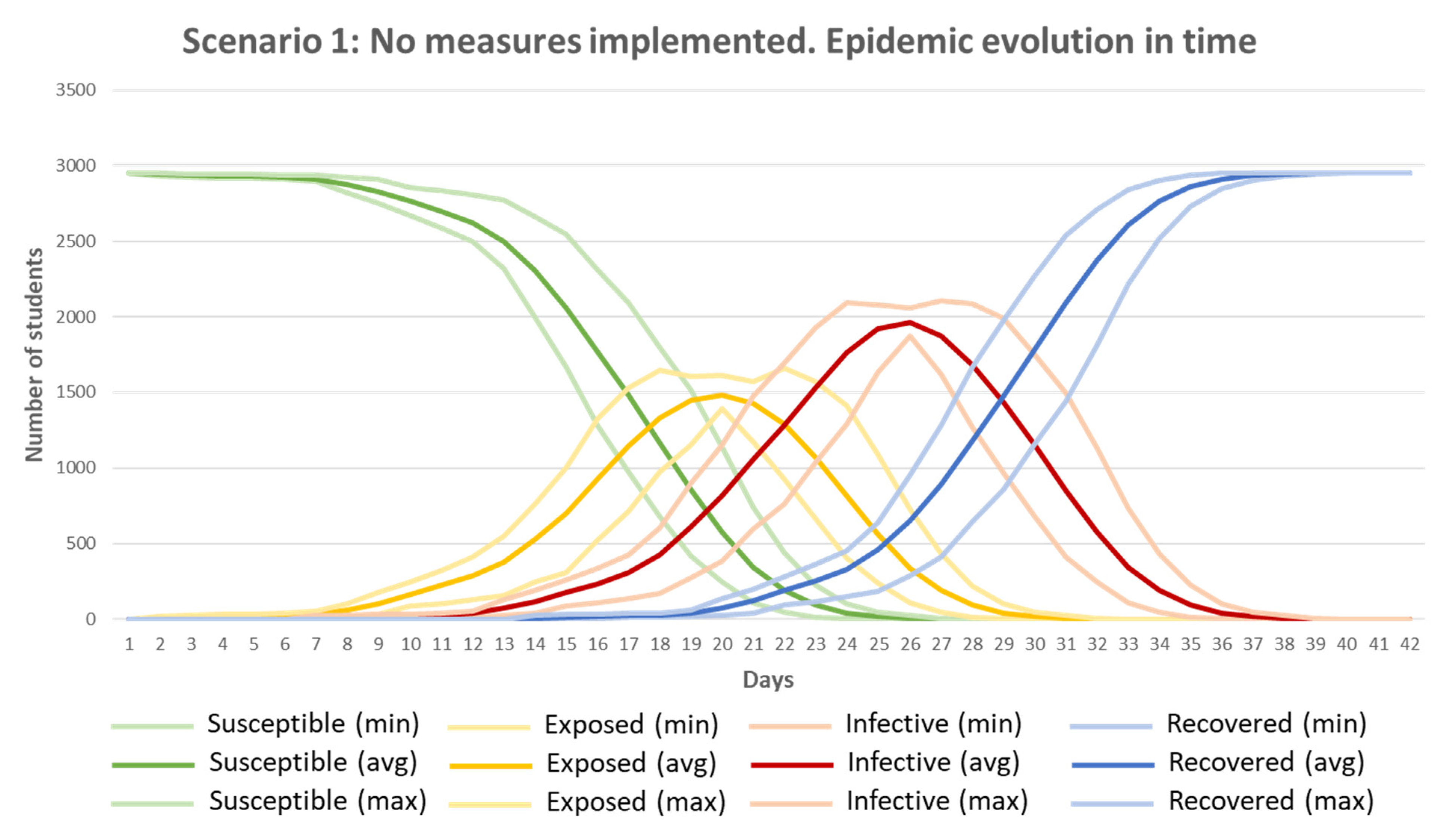
Scenario 1 shows how COVID-19 evolves and behaves in time and space when no measures to reduce the risk are applied. Twenty simulations of Scenario 1 were analysed with the values defined in Table 7, and maximum, minimum and average values were obtained (Figure 13). It can be observed that the number of ‘Susceptible’ agents decreases over time as more students become ‘Exposed’ and ‘Infective’, with most students no longer ‘Susceptible’ by Day 25. The ‘Exposed’ peak value was obtained between Days 17 and 23 (mean Day 20). The peak in ‘Infective’ students was reached between Days 24 and 30 (mean Day 26), with a maximum of two thirds of the population infected (‘Infective’) at the same time. After 40 days, all students (2954) were ‘Recovered’.
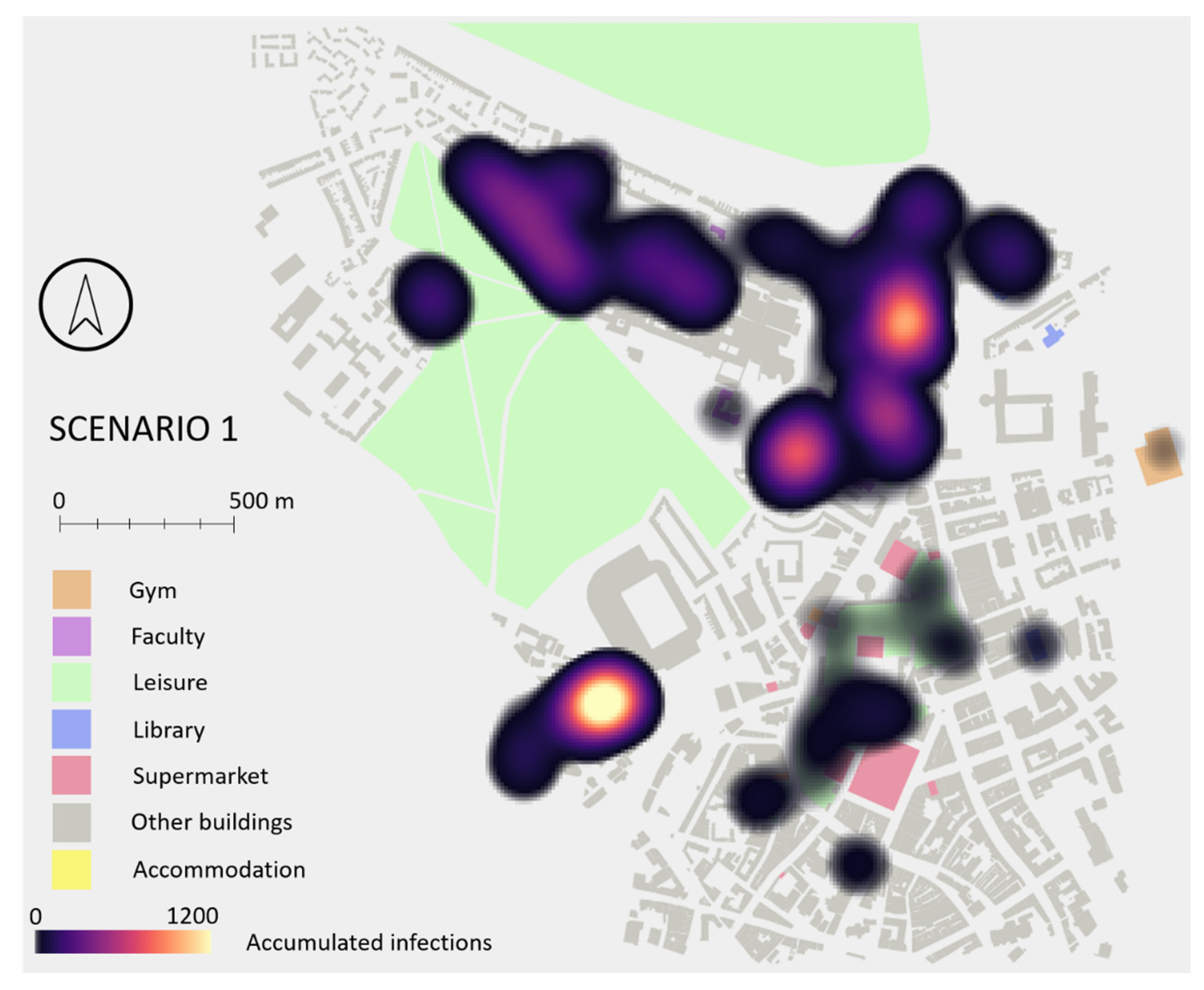
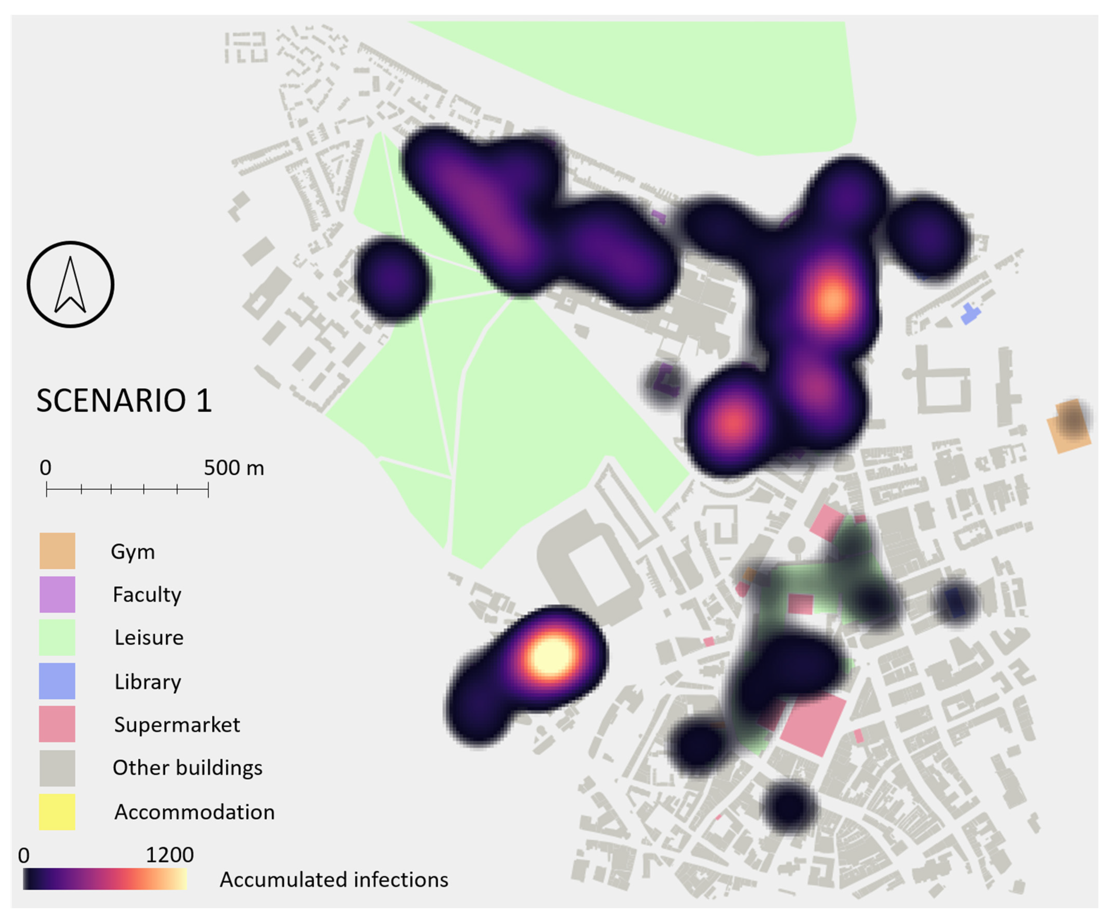
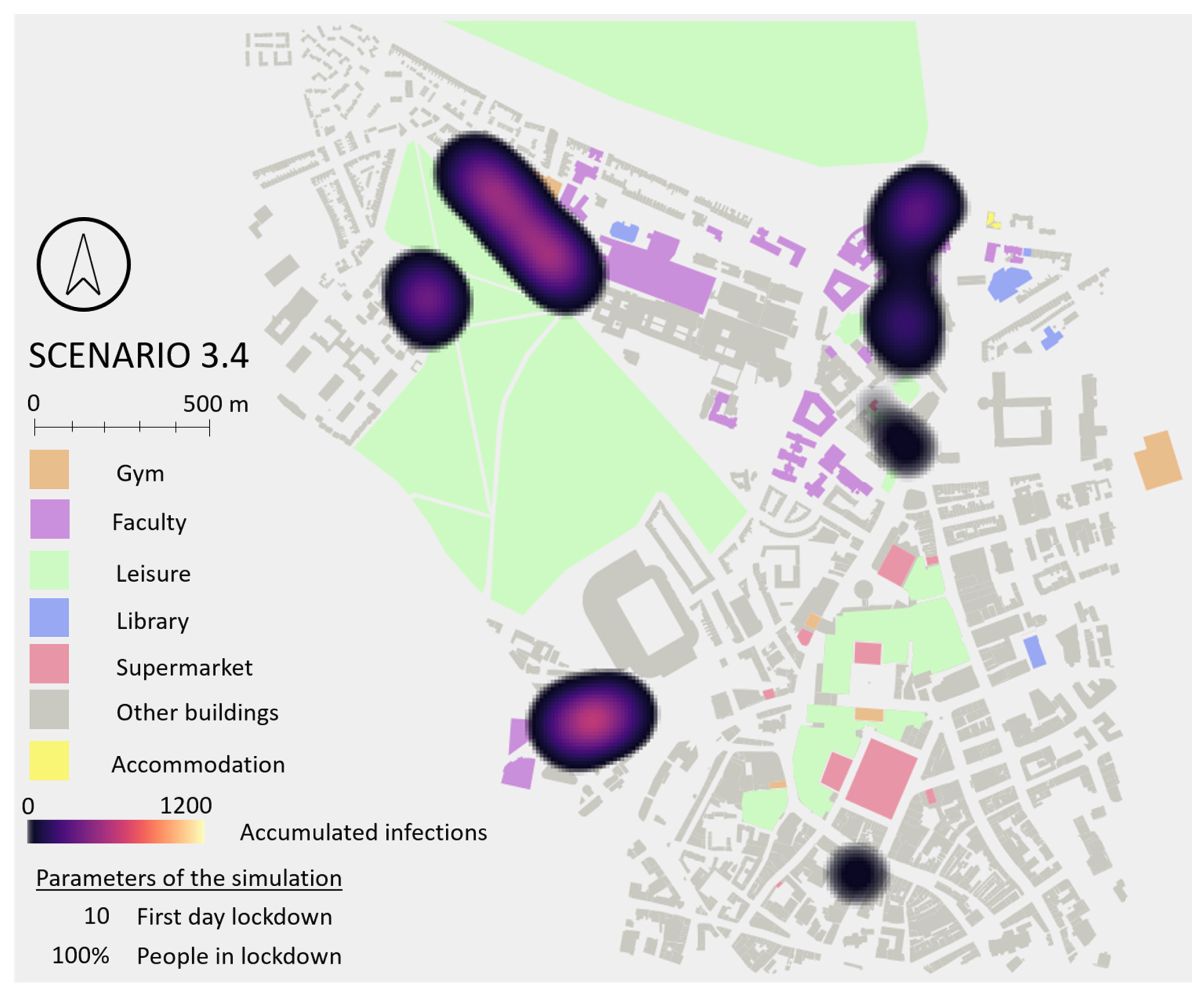
This scenario was also analysed from a spatial perspective. Figure 14 shows a heat map identifying the areas of the city where more infections occurred. Two main hotspots are visible, one in the SE of the study area where two student accommodations and a busy supermarket are located, and one in the main campus where most faculty buildings and another supermarket are located. Accommodations and faculty buildings are where students spend most of their time, while those supermarkets are very small buildings where many of them go at the same time, based on students’ schedules.
3.2. Scenario 2: Facemasks
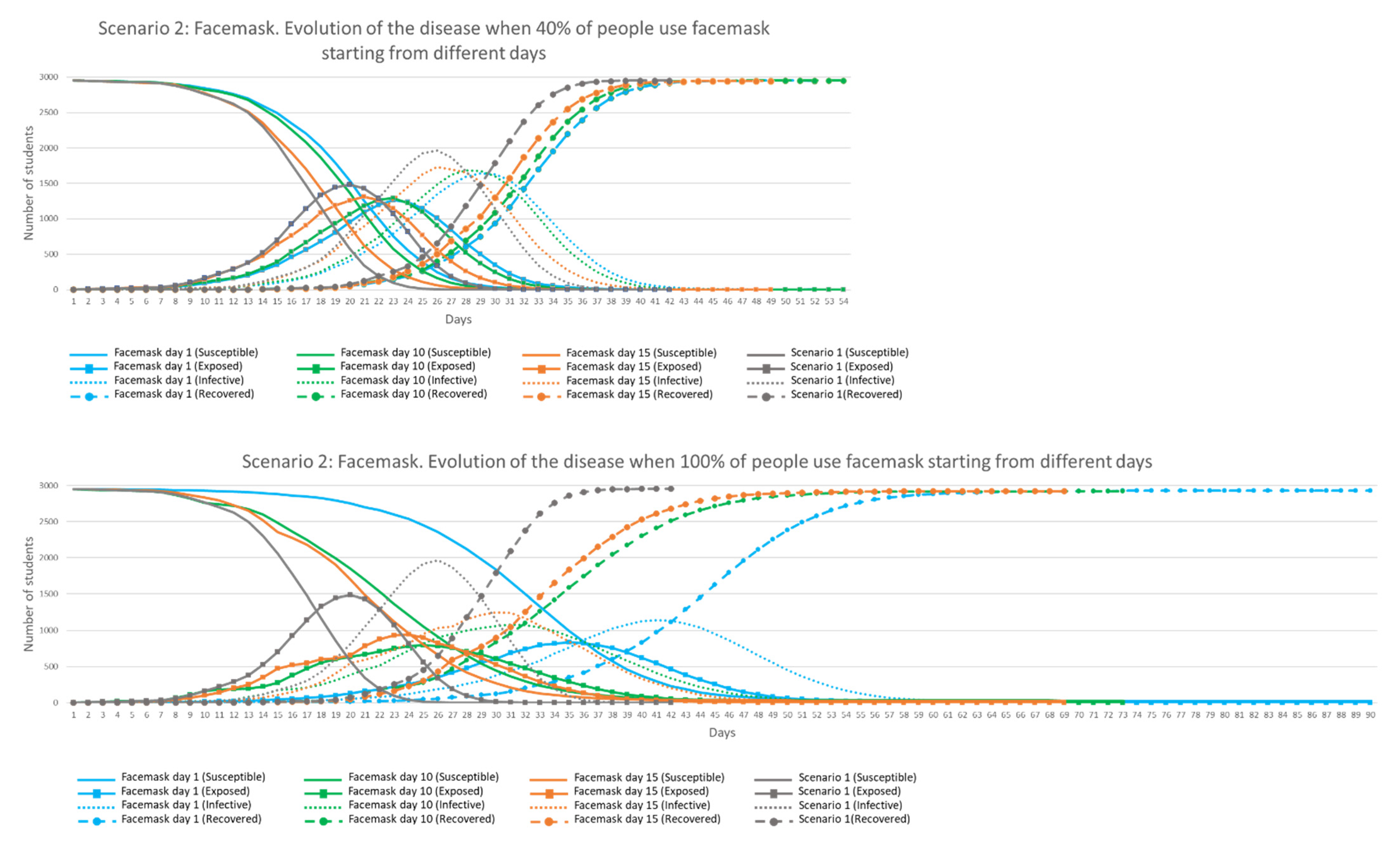
Similar results were generated for the Facemask scenario described in Section 2.6, with the 12 combinations of facemask use simulated four times each. Figure 15 shows the evolution of the disease in time when different percentages of facemask use was adopted by agents from Days 1 (blue), 10 (green) and 15 (orange) of the simulation, compared against results from Scenario 1 (grey).
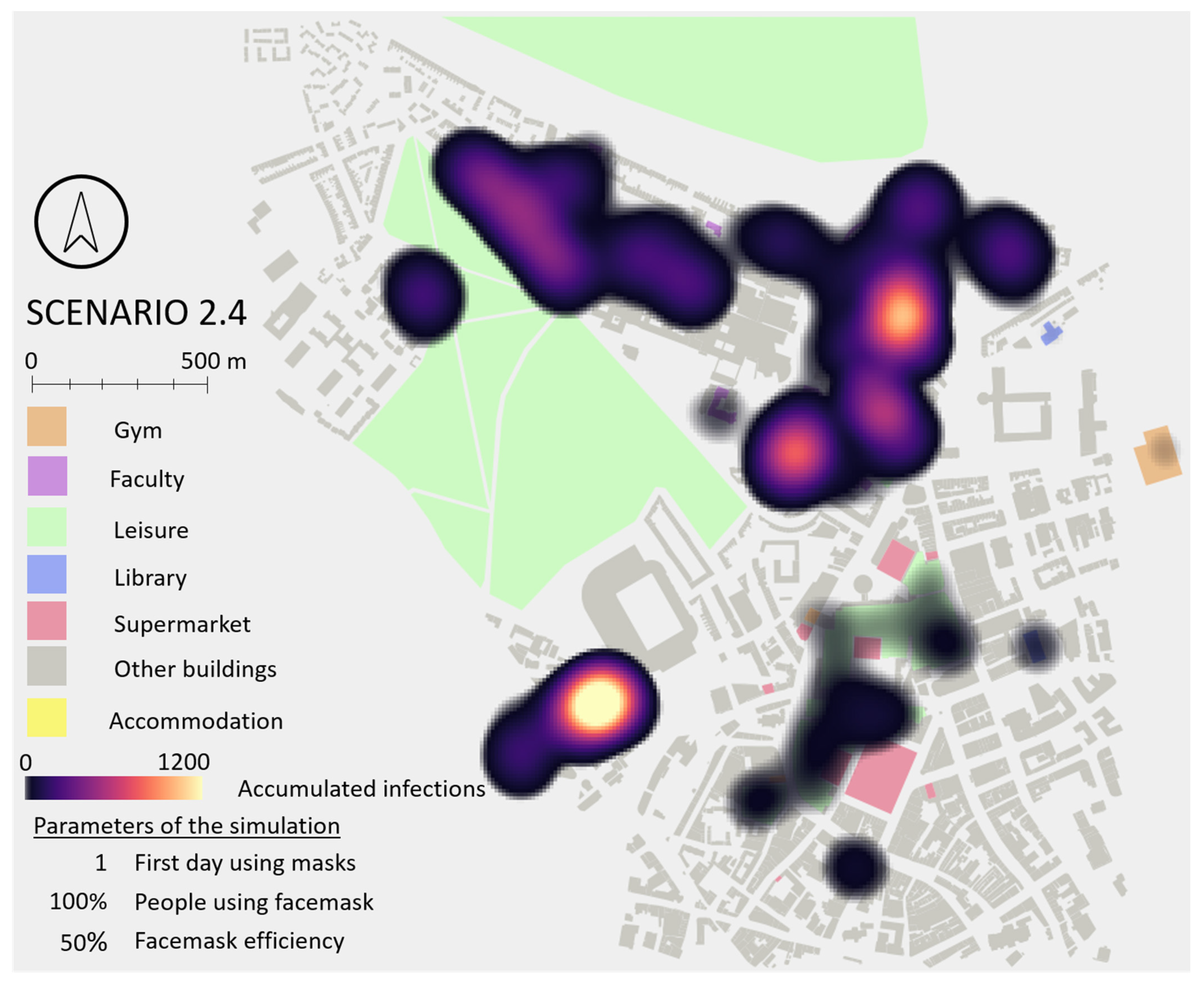
It can be observed in Figure 15 that when only 40% of the students were using facemask (top chart), the behaviour of the disease in the environment was very similar to Scenario 1 with no facemask use. When this percentage was increased to 60, 80 and 100%, more differences were observed in shapes and duration of the disease in the environment. With 100% mask use (bottom chart) the ‘Exposed’ and ‘Infective’ peaks are reached approximately 16 days later when facemasks were used from Day 1 (blue line). When 100% of students used facemasks, the maximum ‘Exposed’ and ‘Infective’ peak values were reduced by 25 and 30% respectively. There are also differences in the required time to eradicate the disease from the environment. More time was needed when more people used facemasks, with 63 days on average being needed with 100% mask use from Day 1. Finally, it was observed that only 1% remained ‘Susceptible’ when 100% were using facemask from Days 1, 10 and 15. This shows that facemasks with 50% efficiency help to flatten the curves but are insufficient to eradicate the disease and reduce the ultimate infection risk. This confirms the observation highlighted by Eikenberry et al. (2020) [39]: ‘masks should not be viewed as an alternative, but as a complement to other public health control measures (including non-pharmaceutical interventions, such as social distancing, self-isolation, etc.)’. Spatial analysis of infection locations revealed no major difference between Scenarios 1 and 2, as daily routines (and therefore locations of major interactions between students) are not altered by the use of facemasks. A spatial hotspot map for Scenario 2 is included in Appendix G.
3.3. Scenario 3: Lockdown
Simulations were undertaken for the Lockdown scenario when different percentages of people stay at home starting from different days of the simulation (see Section 2.6). The combination of these parameters produced twelve simulations, run four times each, in order to find the range of minimum, maximum and average values.
Figure 16 shows a comparison of different percentage of people in lockdown starting from Day 10. The graph shows that curves were flattened even when only 40% were in lockdown (reducing the ‘Exposed’ and ‘Infective’ peaks a third and over a quarter, respectively). The most extreme peak reductions were obtained when 80% were in lockdown but the disease remained longer in the environment (up to 80 days as an average). When all students were in lockdown, peak values were higher than when there were 80% (‘Infective’ students were sharing the apartment with other ‘Susceptible’ students at all times, infecting them), duration shorter (43 days as average) and this kept approximately two thirds of the population away from the disease (students that did not share accommodation with any ‘Infective’ agents). When lockdown started in Day 15, differences between results were less visible and closer to Scenario 1, while when lockdown started just two days later, the results were extremely close to Scenario 1 in shape and time.
The best results were obtained when lockdown started in Day 10, independent of the percentage of people following it. The more people in lockdown, the longer the disease remained in the environment except when all students were at home. Results also suggest that early lockdowns followed by the majority of students keep a higher percentage of students safe from the disease, with a maximum of 65% kept safe when all students are at home from Day 10, and only a 22% when lockdown was raised on Day 15.
Additionally, areas of the city were identified with more infections when different percentage of students were in lockdown from different starting days. The main differences were observed when lockdown started from Day 10 and was followed by everyone, where a more diffuse pattern of infection was found. In the remaining versions of Scenario 3, an increase of cases in accommodation areas and a reduction in faculty buildings were observed due to the students spending more time at home in isolation. Spatial hotspot maps for Scenario 3 is included in Appendix G.
3.4. Scenario 4: Self-Isolation
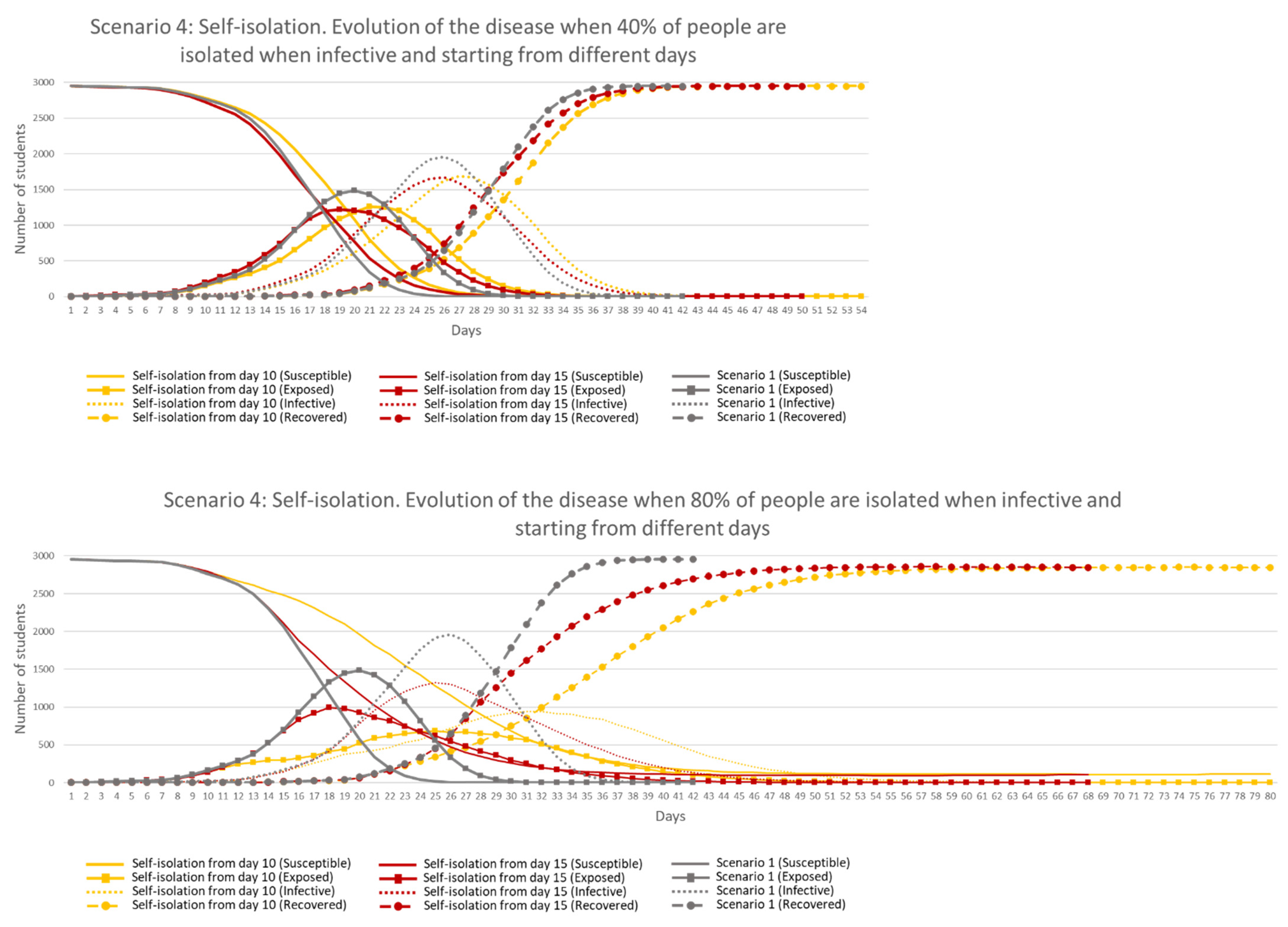
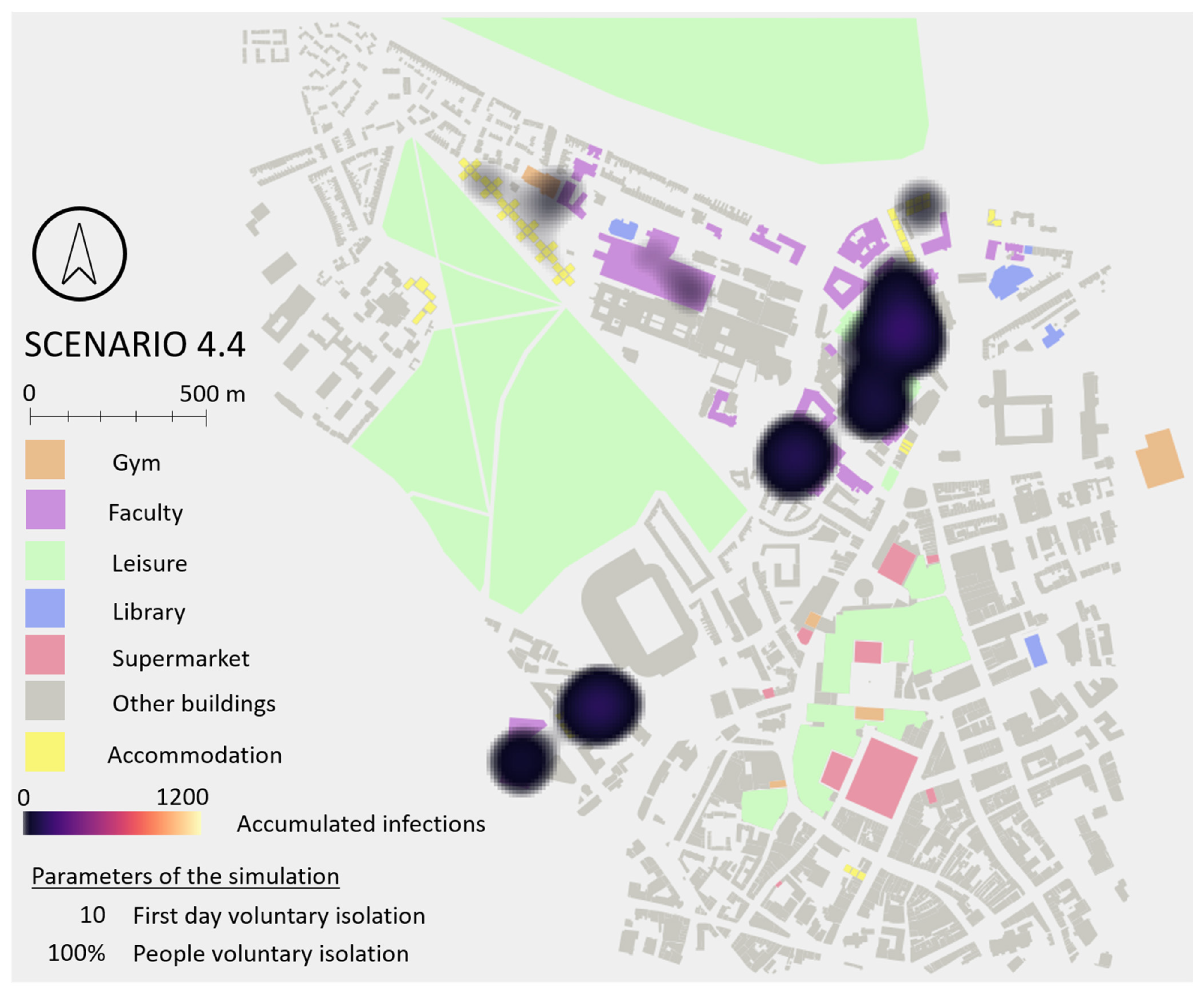
In the self-isolation scenario, ‘Infective’ students voluntarily decided to avoid contact with others by staying at home alone. As described in Section 2.6, various simulations were conducted with differing percentages of self-isolated students starting from different days, generating eight simulations, run four times each. Figure 17 shows the results when the same percentage of student agents were in lockdown starting from different days compared to Scenario 1.
Results show that 40% of self-isolation (top chart) did not have an impact in the results when compared against Scenario 1. It was from a 60% self-isolation when results were visible (only from Day 10), being more efficient when the measure was followed by at least 80% (bottom chart), but staying longer in the environment and keeping only 4 and 3% of the students safe, when starting Days were 10 and 15, respectively. Self-isolation followed by 100% of students provided the best results in both starting days, in terms of peak values, length of the disease in the environment and number of students safe (86% and 58%, starting from Day 10 and 15, respectively). These results highlight the importance of testing people to identify infectiveness and isolating them as soon as possible.
It is important to highlight that even when every ‘Infective’ student was self-isolated, disease transmission continued growing for a few days in both starting day scenarios. This fact occurs because some ‘Exposed’ students became ‘Infective’ but also because some ‘Infective’ static and ‘Contaminated Elements’ remained in the environment with the ability to infect students for one more day. If the percentage of self-isolated students was lower, the effect of ‘Infective’ static and ‘Contaminated Elements’ in the environment was a more important factor in the transmission of the disease. Based on this finding, it can be highlighted the importance of cleaning contaminated areas to reduce the transmission.
When results were analysed spatially, observed hotspots were similar to Scenario 1, keeping the same two main focii, except when 100% of students were self-isolated. In this case, especially starting from Day 10, those focii were not generated because 86% of the students were kept safe and therefore case numbers (and densities) were much lower. This demonstrates that self-isolation does not change the locations of infection unless imposed early (before agents are Infective). Spatial hotspot map for Scenario 4 is included in Appendix G.
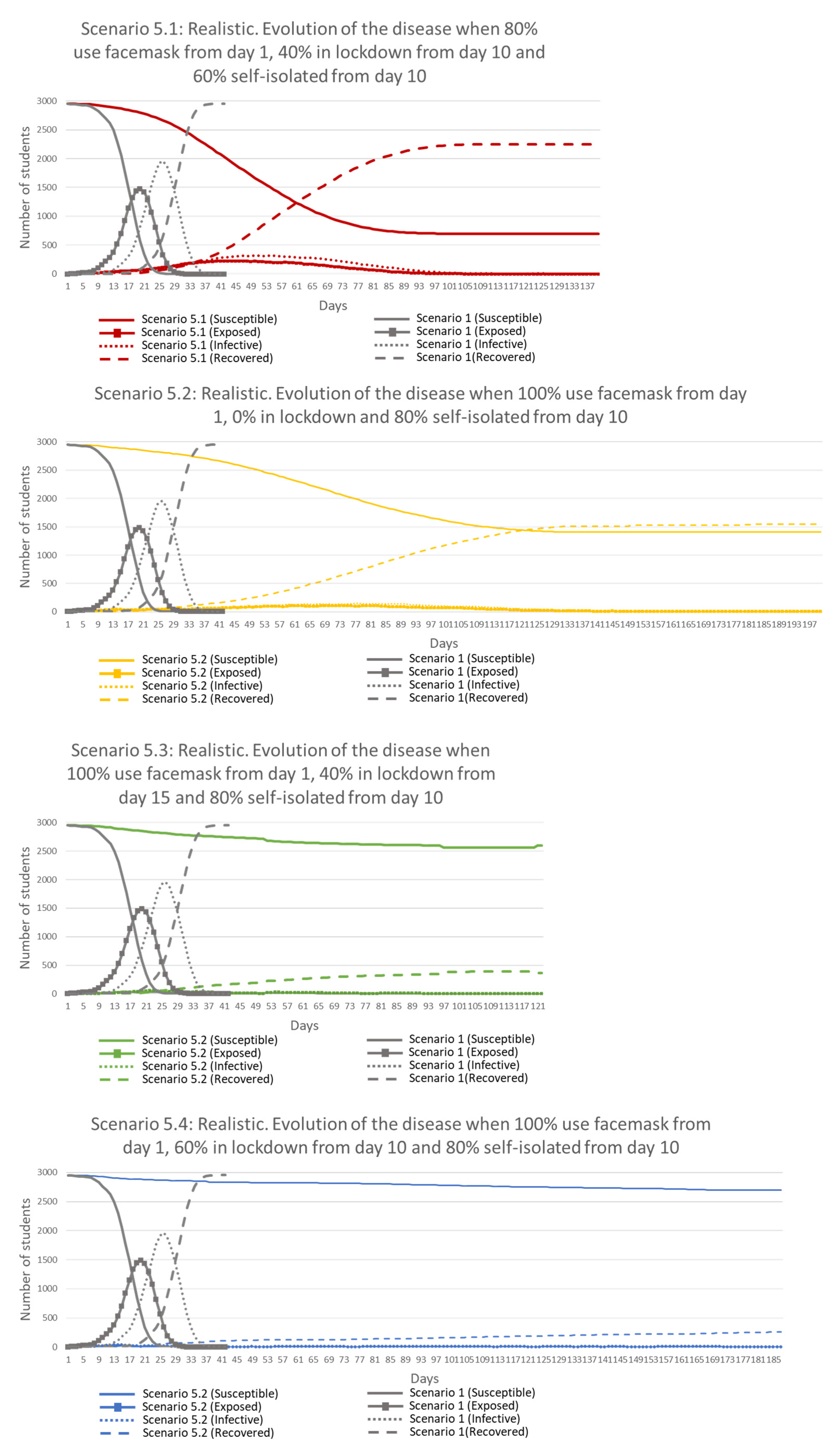
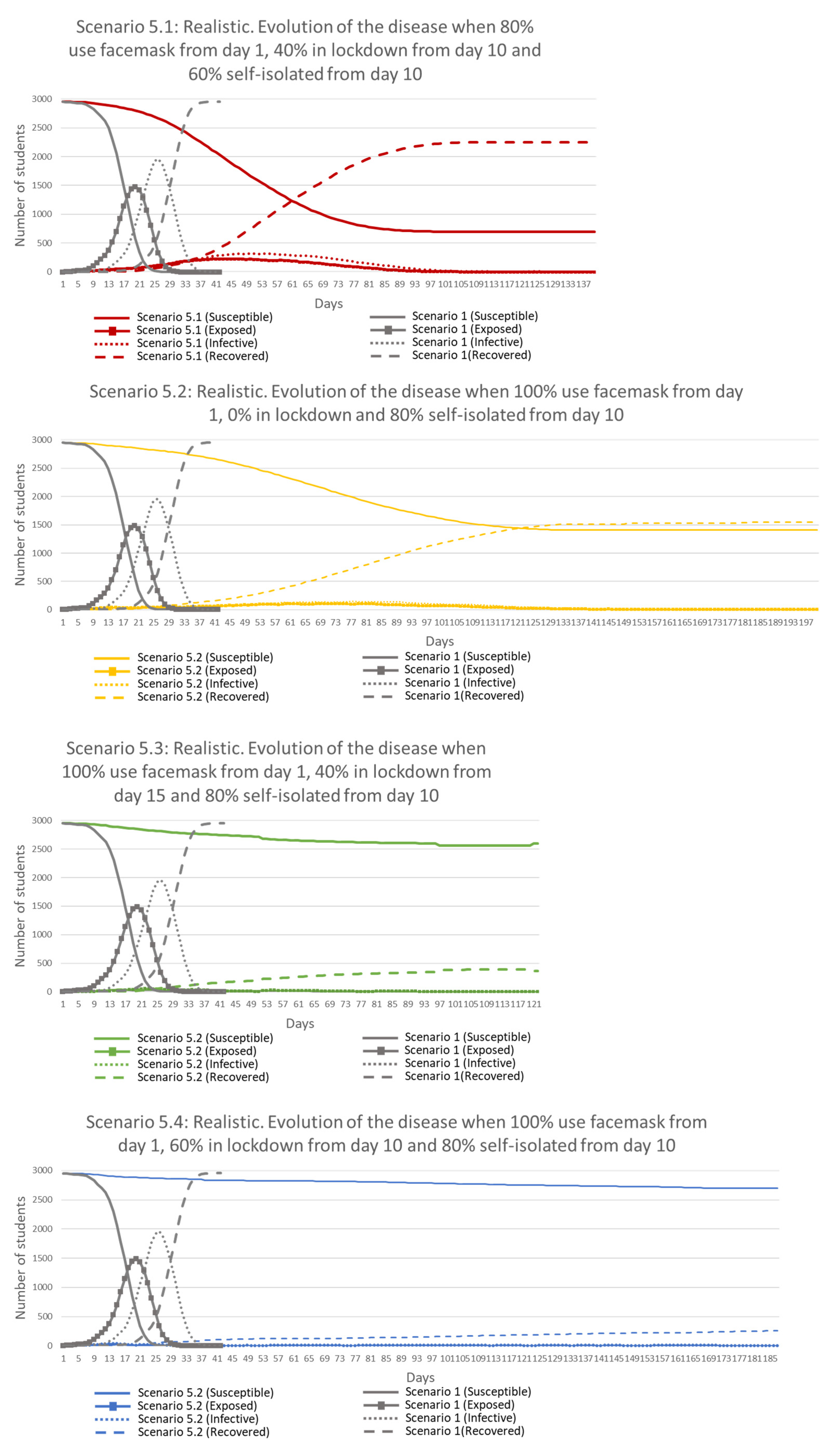
3.5. Scenario 5: Realistic
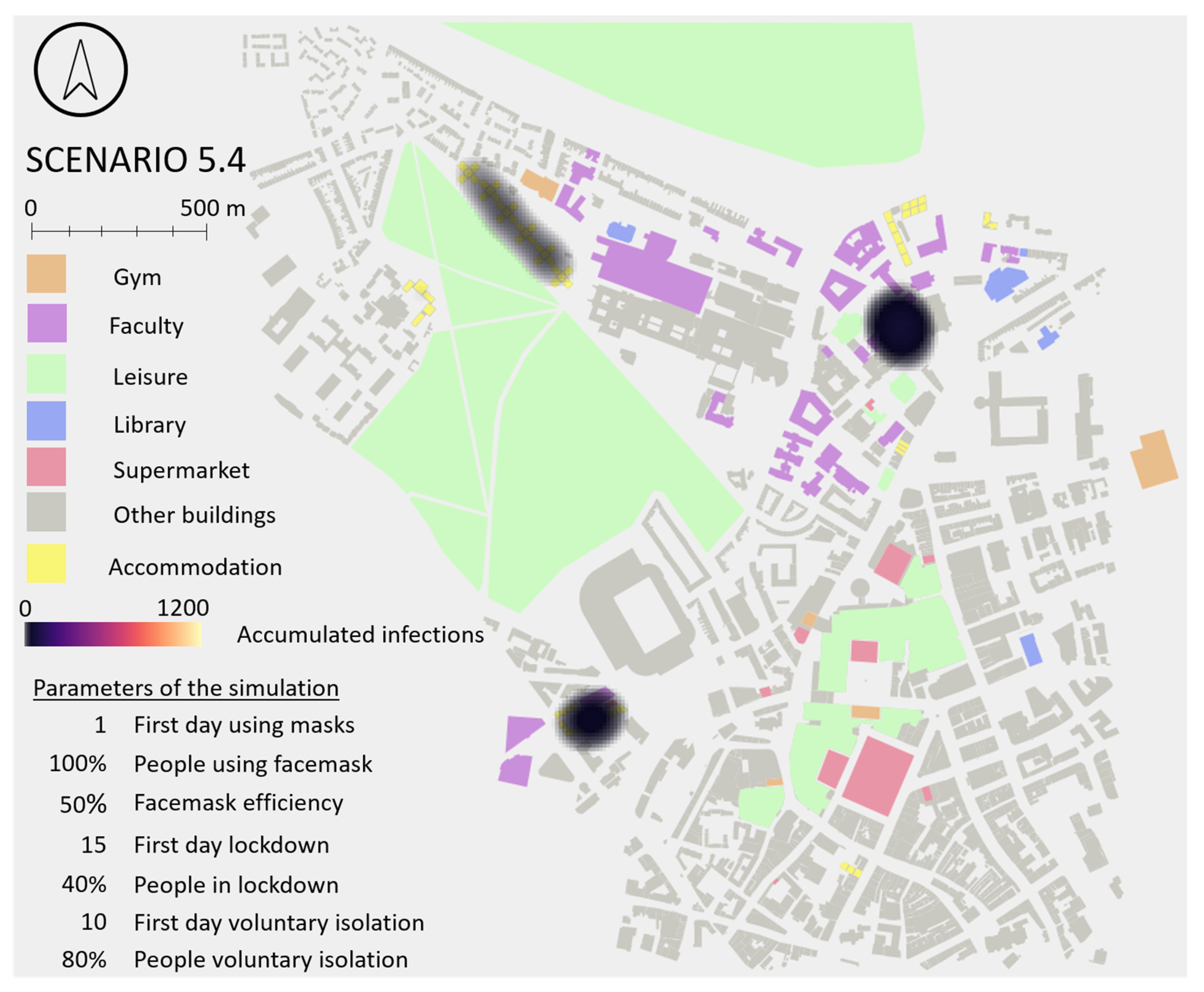
This scenario combines measures from Scenarios 2, 3 and 4 in order to reduce the risk of infection. From previous scenarios, it was observed that facemasks help flattening the curves but not reducing the risk, an efficient lockdown must be deployed early and be followed by most of the population, and self-isolation helps flattening the curves but is only effective when all agents are self-isolated when ‘Infective’. Based on these results, it was decided to create four realistic situations to face COVID-19 (each one simulated four times), combining previous measures with differing percentages of people following each, and applying them from different days. Table 8 specifies the parameters used in each simulation.
Results from Figure 18 show a major improvement from Scenario 1, flattening the curves in all cases and reducing in the worst case the ‘Exposed’ and ‘Infective’ peak values by 45 and 56% respectively (48 and 63% in the best case). This implies extending the presence of the disease in time, especially when lockdown was not deployed (Scenario 5.2). The least restrictive Scenarios (5.1 and 5.2) kept fewer people safe than Scenarios 3.4 and 4.4, where everyone followed lockdown from Day 10 and everyone followed self-isolation from Day 10, respectively. A great improvement in the percentage of safe people from the disease was obtained in the two more restrictive Scenarios (5.3 and 5.4), where on average 90 and 95% of students remained ‘Susceptible’ (and therefore, disease-free) at the end of simulations.
Interesting results were obtained when comparing Scenarios 5.1 and 5.3. More restrictive measures were applied in Scenario 5.3 related to facemasks use and self-isolation but a later lockdown with same percentage of people than in Scenario 5.1. Results showed a five-fold reduction in peak values, 23 days reduction of disease in the environment and 67% more students safe in Scenario 5.3. These results suggest the importance of the facemasks and self-isolation even when lockdown is applied.
Very little and compacted areas of infection were observed when results were analysed spatially in Scenarios 5.3 and 5.4 (mainly in the two areas highlighted in Scenario 1). This is because the number of students that remained susceptible (healthy) at the end of the simulation were 90 and 95%, respectively. Scenarios 5.1 and 5.2 showed closer results to Scenario 1, but with less number of infections (23 and 47% of students remained susceptible at the end of the simulations, respectively). A spatial hotspot map for Scenario 5 is included in Appendix G.
Applied individually, measures are not as effective as when combined, obtaining the best results in Scenario 5.4, when measures with restrictive controls were applied, seeing exposed and infective peak values reduce to 2 and 3% of students respectively, and keeping 95% of students safe from the virus. These results suggest the need of commitment from students to follow the measures with the aim of reducing and minimising infection. Results demonstrated that when even a small percentage of students fail to follow the measures, the risk increases to everyone, obtaining higher ‘Exposed’ and ‘Infective’ peak values and keeping fewer students safe.
Table 9 shows the best obtained result from each of the case-scenarios simulated. Values about the day when ‘Exposed’ and ‘Infective’ peak values were reached, the percentage of students exposed and infective in the ‘Exposed’ and ‘Infective’ peak days, and the percentage of students remaining susceptible at the end of the simulation are compared.
Appendix H shows a table comparing detailed results from all five developed case-scenarios.
4. Discussion and Future Work
The results obtained when simulating a COVID-19 outbreak applying no measures (Scenario 1) showed that disease evolves quickly in time (in less than two weeks the disease was spread to almost all agents), with extremely high ‘Exposed’ and ‘Infective’ peak values (half and two thirds of the population, respectively).
The ‘Facemask’ scenario (Scenario 2) showed that the use of facemasks (50% efficiency) helps to ‘flatten the curves’ and increase the duration of the disease in the environment but does not reduce the ultimate risk of infection. Higher mask use results in lower ‘Exposed’ and ‘Infective’ peak values (a reduction of 25 and 30%, respectively in the best case-scenario), but at the end of simulations just 1% of students remained uninfected. Clearly, the actual efficacy of facemasks will vary from the 50% simulated in this paper and the effect of more efficient facemasks should be considered.
The ‘Lockdown’ scenario (Scenario 3) showed an important reduction of ‘Exposed’ and ‘Infective’ peak values (29 and 40%, respectively) and a high percentage of people kept away from the disease (65% in the best case) when lockdown was followed by everyone and if it was raised early (Day 10). If lockdown was deployed later, its efficiency was reduced considerably in all terms, being similar or even worse than when measures were not applied. This suggests that governments or university management must be brave and pro-active when applying lockdowns if they are to be effective.
The ‘Self-Isolation’ scenario (Scenario 4) showed that, when at least 60% or 80% of ‘Infective’ students self-isolated from Days 10 or 15, the ‘Exposed’ and ‘Infective’ peak values were reduced considerably. The student community was only kept safe, however, if every ‘Infective’ person self-isolated; if a small percentage of ‘Infective’ agents continued their normal routines then the disease continued spreading and a very small percentage of the population was kept safe. These results show the importance of testing, in order to identify ‘Infective’ people and isolate them as soon as possible.
The ‘Realistic’ scenario (Scenario 5), showed a remarkable reduction in peak values (down to 2 and 3% of ‘Exposed’ and ‘Infective’ peaks) and an impressive percentage of people kept safe (95% in the best case). The disease, however, stayed longer in the environment (the average duration was around three times Scenario 1). The more restrictive the parameters used, the better results were obtained. The scenarios simulated in the model showed the variable importance of each measure depending on their efficiency, the percentage of students following them, and the starting day. All four restrictions simulated (i.e., facemask use, lockdown, self-isolation and realistic) reduce the peak values (exposed and infective) and the number of infected agents, but only one delays the exposed and infective peak values (facemask use) (see Table 9). In this scenario, students’ daily routines are not altered (only the probability to be infected is modified by those wearing a facemask). In the rest of the scenarios: (1) measures applied are more restrictive than just waring a facemask; (2) daily routines are altered and fewer interactions are generated between students (especially with those that do not share accommodation); and (3) restrictions are applied early in time. The best results were obtained when lockdown, self-isolation and realistic scenarios were applied in Day 10 (10 days earlier than the exposed peak value was reached in Scenario 1). Restrictions arrested the increase of the disease between the agents, reaching the peak values faster with a much lower percentage of agents affected.
It was also observed that measures implemented in isolation are not as effective as when combined. It is required that a realistic percentage of people follow several measures at the same time to reduce the risk, flatten the curves and keep as many people as possible safe. Commitment between society and governments is required when applying measures to reduce the transmission.
The results obtained from the modelling in this paper suggest that ABMs are useful tools for simulating the spread of the COVID-19 disease in populations such as students, as results obtained are analogous to those obtained by other researchers in papers cited above in the Introduction section. Each scenario was simulated a limited number of times, which may affect the quality and quantity of final results due to the stochasticity of the model outputs. Further simulations should be conducted in order to perform a true sensitivity analysis and identify these ranges more precisely. Additionally, it was not possible to perform a validation of results against reality. Currently, the pandemic is still spreading in the world and reliable data are difficult to obtain, especially data related to the number of people infected (the majority of the population does not require healthcare and these cases are not counted in the statistics). In the future, when more information about the disease and the impact in population is known, it could be possible to compare results and identify how accurate these scenarios are. Additionally, the study area is considered a closed system, where only students living in student accommodations and a limited number of other persons are simulated. Clearly, in reality, students will interact with additional agents from outside the university environment, but this assumption was required in order to study the spread of the disease (and measures adopted) amongst the student population. This is a limitation that must be considered when analysing the results.
Future work could extend the ABM in a number of ways to improve results and obtain a better understanding of the transmission in space and time. These may include:
- Eliminate some of the assumptions and limitations in the model, such as additional variation of the population including different severities and asymptomatic cases.
- Develop students’ daily routines based on real data and not based on assumptions. The use of mobile phone locations, daily registers of students at faculties and the average number of customers in supermarkets, among many others, could generate realistic daily routines. These routines could simulate accurate spatial interactions and a more precise understanding of the spread could be achieved.
- Comparison of disease numbers against local hospital capacity to set targets for avoiding overwhelming health services with severe cases.
- Simulation of additional measures to reduce the risk, such as social distancing and regular cleaning of contaminated elements.
- Develop spatial analyses more exhaustively in order to identify more patterns and differences between scenarios, applying spatial statistics and other spatial techniques.
- Extrapolate the model to the entire population of a city (not only students). This would clearly be dependent on availability of data (see above) and computing power.
5. Conclusions
This paper presented the development of an ABM to simulate the spread of COVID-19 and explored the transmission of the disease from a geospatial perspective to identify potential measures to reduce infection within students living in student accommodation. The model demonstrated that it is possible to combine spatial data and a mathematical epidemic model in ABMs to capture the dynamics of the spread of an infectious disease, with results analogous to those simulated by other models. The paper demonstrated the use of the GAMA platform for developing a 3D ABM of buildings, footpaths, students, other dynamic and static agents. Their interactions, based on daily routines, and the implementation of a mathematical epidemiological SEIR model, allowed the simulation of generic outbreaks in the area of study.
This ABM is a customisable and versatile tool that can be used to simulate different infectious disease scenarios when parameters of the disease are known. Additionally, the model can be applied to other areas of the world where geospatial data related to the agents (such as home locations and routines) are available, following the structure shown in Appendix B. The use of ‘Static’ and ‘Contaminated Element’ agents in the model adds an additional layer of complexity to the analysis of the spread of an infectious disease, simulating the effect of contaminated areas and surfaces.
The model also simulated disease prevention measures to test their efficiency in reducing the risk of infection when a COVID-19 outbreak occurs in the area of study. The ABM code was implemented with measures such as the use of facemasks, the deployment of lockdown and the ability of self-isolation when ‘Infective’. These measures were simulated individually and combined, applying them to different percentage of students and starting them from different days.
Spatial analyses in all scenarios showed that the most dangerous places were those where many students interact for a long time (university buildings and accommodation) and small buildings where many go at the same time (most popular supermarkets). The use of this type of model and analysis of outputs could help medical practitioners and university managers to respond to such epidemics and plan effective responses to keep as many students safe as possible.
Author Contributions
Conceptualization, David Alvarez Castro and Alistair Ford; methodology, David Alvarez Castro and Alistair Ford; software, David Alvarez Castro; validation, David Alvarez Castro and Alistair Ford; formal analysis, David Alvarez Castro; investigation, David Alvarez Castro; resources, David Alvarez Castro; data curation, David Alvarez Castro; writing—original draft preparation, David Alvarez Castro; writing—review and editing, Alistair Ford; visualization, David Alvarez Castro and Alistair Ford; supervision, Alistair Ford; project administration, David Alvarez Castro. All authors have read and agreed to the published version of the manuscript.
Funding
This research was funded by EPSRC Centre for Doctoral Training in Geospatial Systems, Grant Number EP/S023577/1.
Institutional Review Board Statement
Not applicable.
Informed Consent Statement
Not applicable.
Data Availability Statement
A repository containing code and GIS datasets used in the project is at https://github.com/DACNC/ABM_COVID19_Students_Transmission (accessed on 21 May 2021). Some data requires Ordnance Survey license.
Acknowledgments
The authors would like to thank Paul Goodman for his help in the development of the methodology used in this paper.
Conflicts of Interest
The authors declare no conflict of interest. The funders had no role in the design of the study; in the collection, analyses, or interpretation of data; in the writing of the manuscript, or in the decision to publish the results.
Appendix A
Table A1 shows the comparison of different open-source ABM platforms to develop a 3D geospatial epidemic model.

Table A1.
Open source ABM comparison.
| Characteristic | Repast | GAMA | NetLogo |
|---|---|---|---|
| Purpose | Multiple application domains (e.g., Transport Urban planning Epidemiology Environment) | Multiple application domains (e.g., Transport Urban planning Epidemiology Environment) | Multi-agent programmable modeling environment. |
| Urban mobility | Yes | Yes | Yes |
| Epidemiology | Yes | Yes | Yes |
| Language | ReLogo and Java | GAML | Logo dialect |
| Documentation | Yes | Yes | Yes |
| Tutorials | Yes | Yes | Yes |
| User guide | Yes | Yes | Yes |
| Mailing and contact list | Yes | Yes | Yes |
| License | Free and open-source agent-based modeling and simulation platforms ‘New BSD’ style license: | GNU General Public License v3.0 | GNU General Public License, version 2 or any later version |
| License link | https://repast.github.io/license.html (accessed on 26 July 2020) | https://github.com/gama-platform/gama/blob/master/LICENSE (accessed on 26 July 2020) | https://ccl.northwestern.edu/netlogo/docs/copyright.html (accessed on 26 July 2020) |
| Input data format | Excel, shapefiles, raster | Shapefiles, rasters and others | GIS extensions, text files, CSV and others |
| Export data format | Microsoft Excel (xlsx, csv) | ASC, CSV, GeoJson, Geotiff, KML, PNG, SHP, Text, shapefile | Plain-text and CSV |
| Agents type | The agents are individual people in the innovation network | Buildings, roads, people and any other agent representing an element in the space and/or with skills | Four types of agents: turtles, patches, links, and the observer |
| Visualisation | Yes | Yes | Yes |
| Use of PostgreSQL Db (Data Management) | - | Yes | - |
| Several experiments simultaneously | - | Yes | - |
| Sources | https://repast.github.io/ (accessed on 26 July 2020) | https://gama-platform.github.io/wiki/Home (accessed on 26 July 2020) | https://ccl.northwestern.edu/netlogo/ (accessed on 26 July 2020) |
Appendix B
GIS attribute tables of students (Table A2), footpaths (Table A3), buildings (Table A4), dynamics (Table A5) and static (Table A6) agents. Attribute names, type of attributes, examples, notes and considerations are defined for each of them. These tables can be generated in a GIS software (e.g., QGIS) or in a PostGIS database.
Table A2.
GIS attribute table of Students.
| Attribute | Type | Example | Notes | Considerations |
|---|---|---|---|---|
| id | String | S100 | Unique value. PK | ‘S’ + unique integer |
| residence | String | Park_Terrace | Accommodation’ s name | - |
| init_floor | Integer | 3 | Floor number | - |
| t1_even | String | Faculty_1 | Building’s name for Task 1 in even days | - |
| t1_t_even | Integer | 510 | Minute in which student starts Task 1 in even days | Time in minutes (0–1439) |
| t2_even | String | Gym_1 | Building’s name for Task 2 in even days | - |
| t2_t_even | Integer | 700 | Minute in which student starts Task 2 in even days | Time in minutes (0–1439) |
| t3_even | String | Supermarket | Building’s name for Task 3 in even days | - |
| t3_t_even | Integer | 800 | Minute in which student starts Task 3 in even days | Time in minutes (0–1439) |
| t4_even | String | Library_2 | Building’s name for Task 4 in even days | - |
| t4_t_even | Integer | 900 | Minute in which student starts Task 4 in even days | Time in minutes (0–1439) |
| home_t_e | Integer | 1230 | Minute in which student goes home in even days | Time in minutes (0–1439) |
| t1_odd | String | Library_3 | Building’s name for Task 1 in odd days | - |
| t1_t_ odd | Integer | 520 | Minute in which student starts Task 1 in odd days | Time in minutes (0–1439) |
| t2_ odd | String | Gym_3 | Building’s name for Task 2 in odd days | - |
| t2_t_ odd | Integer | 830 | Minute in which student starts Task 2 in odd days | Time in minutes (0–1439) |
| t3_ odd | String | Faculty_1 | Building’s name for Task 3 in odd days | - |
| t3_t_ odd | Integer | 950 | Minute in which student starts Task 3 in odd days | Time in minutes (0–1439) |
| t4_ odd | String | Leisure_4 | Building’s name for Task 4 in odd days | - |
| t4_t_ odd | Integer | 1000 | Minute in which student starts Task 4 in odd days | Time in minutes (0–1439) |
| home_t_o | Integer | 1235 | Minute in which student goes home in odd days | Time in minutes (0–1439) |
| geom | Geometry | - | Point 2D (Point) | - |
Table A3.
GIS attribute table of footpaths.
| Attribute | Type | Example | Notes | Considerations |
|---|---|---|---|---|
| id | Integer | 1 | Unique value. PK | Exploded lines |
| geom | Geometry | - | Line 2D (LineString) | - |
Table A4.
GIS attribute table of buildings.
| Attribute | Type | Example | Notes | Considerations |
|---|---|---|---|---|
| id | Integer | 1 | Unique value. PK | Exploded lines |
| type | String | Faculty | Type of building (faculty, residence, gym, leisure, supermarket, library, other) | - |
| faculty | String | Medical_Science | Name of the faculty to which the building belongs to | If building type is not faculty, this attribute is black |
| name | String | Faculty_1 | Name of the building | - |
| bui_floor | Integer | 4 | Number of floors | Ground floor is 0 |
| bui_speed | float | 0.010 | Speed (m/s) agents can move when inside the building | - |
| geom | Geometry | - | Polygon 2D (Multi-polygon) | - |
Table A5.
GIS attribute table of dynamics.
| Attribute | Type | Example | Notes | Considerations |
|---|---|---|---|---|
| id | String | D1 | Unique value. PK | ‘D’ + unique integer |
| init_floor | Integer | 3 | Floor number where the agent is located | - |
| geom | Geometry | - | Point 2D (Point) | - |
Table A6.
GIS attribute table of statics.
| Attribute | Type | Example | Notes | Considerations |
|---|---|---|---|---|
| id | String | X1 | Unique value. PK | ‘X’ + unique integer |
| init_floor | Integer | 3 | Floor number where the agent is located | - |
| geom | Geometry | - | Point 2D (Point) | - |
Appendix C
Tables providing information about the structure of the output files generated once simulations are finished: ABM_SEIR_values_per_day.csv (Table A7), Agents_after_simulations.csv (Table A8) and Transmission_list.csv (Table A9).
Table A7.
ABM_SEIR_values_per_day.csv attribute table.
| Attribute | Type | Example | Notes | Considerations |
|---|---|---|---|---|
| day_of_simulation | Integer | 8 | Day of the simulation | Simulation’s first day is 1 |
| nb_S_students | Integer | 2500 | Number of ‘Susceptible’ students | - |
| nb_E_students | Integer | 245 | Number of ‘Exposed’ students | - |
| nb_I_students | Integer | 23 | Number of ‘Infective’ students | - |
| nb_R_students | Integer | 4 | Number of ‘Recovered’ students | - |
| contaminated_elements | Integer | 20 | Number of total contaminated elements generated | - |
Table A8.
Agents_after_simulations.csv attribute table.
| Attribute | Type | Example | Notes | Considerations |
|---|---|---|---|---|
| id | String | S41 | Unique value. PK | - |
| type | String | Student | Only students are stored in this table | - |
| t1_even | String | Faculty_1 | Building’s name for Task 1 in even days | - |
| t2_even | String | Gym_2 | Building’s name for Task 2 in even days | - |
| t3_even | String | Supermarket_1 | Building’s name for Task 3 in even days | - |
| t4_even | String | Library_2 | Building’s name for Task 4 in even days | - |
| t1_odd | String | Library_2 | Building’s name for Task 1 in odd days | - |
| t2_odd | String | Gym_2 | Building’s name for Task 2 in odd days | - |
| t3_odd | String | Faculty_1 | Building’s name for Task 3 in odd days | - |
| t4_odd | String | Leisure_4 | Building’s name for Task 4 in odd days | - |
| is_susceptible | Boolean | FALSE | True if student is ‘Susceptible’ | - |
| is_exposed | Boolean | FALSE | True if student is ‘Exposed’ | - |
| is_infective | Boolean | FALSE | True if student is ‘Infective’ | - |
| is_recovered | Boolean | TRUE | True if student is ‘Recovered’ | - |
| infective_contact_counter | Integer | 5 | Number of times the student was in contact with an ‘Infective’ before becoming exposed | - |
| infected_x | Integer | 423909.118 | Coordinate x where student was infected | Dependent of the used EPSG code |
| infected_y | Integer | 565205.819 | Coordinate y where student was infected | Dependent of the used EPSG code |
| infected_z | Integer | 12 | Coordinate z where student was infected | ground level = 0 m |
| exposed_minute | Integer | 815 | Minute of the day when student becomes exposed | - |
| exposed_day | Integer | 86 | Day of the year when the student becomes exposed | - |
| infected_by | Integer | S46 | Id value of the agent that infected him/her | - |
| infective_day | Integer | 91 | Day of the year when the student becomes ‘Infective’ | - |
| infective_minute | Integer | 815 | Minute of the day when student becomes ‘Infective’ | - |
| is_using_facemask | Boolean | FALSE | True if the agent is using facemask | Only when the use of facemask is considered |
Table A9.
Transmission_list.csv attribute table.
| Attribute | Type | Example | Notes | Considerations |
|---|---|---|---|---|
| id | String | D123 | All agents (students, dynamics and statics) are stored | - |
| type | String | Dynamic | Type of the agent (students, dynamics and statics) | - |
| infected_by | String | S145 | Id value of the agent that infected him/her | - |
Appendix D
Research documents read in order to find an appropriate β indoor value for this project. As it can be observed in Table A10, there are many differences between the probability infection values (β) given at each paper.
Table A10.
Probability infectious value (β) comparison between different research projects.
| Source | Epidemic Model | Prob. Infection (β) | Incubation Period (σ) (Days) | Recovery Period (γ) (Days) |
|---|---|---|---|---|
| [13] | ABM-SEIIRDM | 0.1 | 5 | 10 |
| [45] | SEIR | Time dependent | 5.1 | 11.36 |
| [46] | SEIR | Based on reproductive number R0 | 5.2 | 2.3 |
| [47] | SEIR | 0.1 | 7 | 10.25 |
| [48] | SEIR | 8.68 × 10⁻⁸ | 0.631 | 0.1 |
| [49] | SEIRNDC | Range {0.5944, 1.68} | 3 | 5 |
| [50] | SEIR | Scaled to the right value of R0 | 6.4 | 3 or 7 |
| [51] | SEIR | 0.1 | 7 | 10.25 |
| [52] | SEIR | 3.11 × 10⁻⁸/person/day | 7 | 15 |
Appendix E
Table A11.
ABM software requirements.
| Requirements |
|---|
| GAMA Platform, version 1.8 (released on the 31 July 2019) (https://gama-platform.github.io/download) (accessed on 18 May 2020). |
| Java 8 64 bits |
| Update environmental variables: PATH variable should contain an option pointing to folder: /Java/jre1.8.0_171/bin |
Table A12.
Characteristics of the laptop used in the research project.
| Laptop Characteristics |
|---|
| Processor Intel® Core™ i7-8650 CPU @ 190 GHz 2.11 GHz |
| 32.0 GB memory RAM |
| 4 cores |
In total, approximately 289 h were required to obtain the results of the simulated scenarios (simulation tests and validations excluded from these hours).
Appendix F
Comparison of the evolution of the disease between Scenarios 2 (Figure A1), 3 (Figure A2), 4 (Figure A3) and 5 (Figure A4) against Scenario 1.
Figure A1.
Comparison of the evolution of the disease between Scenarios 2 (Facemask Use) against Scenario 1 (No Measures).
Figure A1.
Comparison of the evolution of the disease between Scenarios 2 (Facemask Use) against Scenario 1 (No Measures).


Figure A2.
Comparison of the evolution of the disease between Scenarios 3 (Lockdown) against Scenario 1 (No Measures).
Figure A2.
Comparison of the evolution of the disease between Scenarios 3 (Lockdown) against Scenario 1 (No Measures).

Figure A3.
Comparison of the evolution of the disease between Scenarios 4 (Self-Isolation) against Scenario 1 (No Measures).
Figure A3.
Comparison of the evolution of the disease between Scenarios 4 (Self-Isolation) against Scenario 1 (No Measures).

Figure A4.
Comparison of the evolution of the disease between Scenarios 5 (Realistic) against Scenario 1 (No Measures).
Figure A4.
Comparison of the evolution of the disease between Scenarios 5 (Realistic) against Scenario 1 (No Measures).

Appendix G
Spatial hotspot maps obtained from Scenarios 1 (Figure A5), 2 (Figure A6), 3 (Figure A7), 4 (Figure A8) and 5 (Figure A9). These figures show the best obtained result for each scenario in terms of reduction of the number of infections.
Figure A5.
Heat map for Scenario 1 showing the areas (in light yellow) where more infections were produced. Two main hotspots are visible, one in the SE where two student accommodations and a busy supermarket are located, and the other in the main campus where most faculty buildings and another busy supermarket are located. Contains Ordnance Survey data © Crown copyright and database right 2020.

Figure A6.
Heat map for Scenario 2.4 (100% facemask use from Day 1) showing the areas (in light yellow) where more infections were produced. No major difference can be observed between Scenarios 1 and 2, as daily routines (and therefore locations of major interactions between students) are not altered by the use of facemasks.

Figure A7.
Heat map for Scenario 3.4 (100% students in lockdown from Day 10) showing the areas (in light yellow) where more infections were produced. A reduction in both main areas highlighted in Scenario 1 can be observed, as less infections are produced due to the implementation of the lockdown. Accommodation buildings remain with a high level of infection due to students’ schedule was cancelled, spending the whole day in the accommodation. © Crown copyright and database right 2020.

Figure A8.
Heat map for Scenario 4.4 (100% students self-isolated from Day 10) showing the areas (in light yellow) where more infections were produced. Weak infection areas were found in the study area. As a consequence of self-isolation measure, 86% of students remained susceptible and therefore case numbers (and densities) were much lower. © Crown copyright and database right 2020.

Figure A9.
Heat map for Scenario 5.4 (100% students using facemask from Day 10; 60% of students in lockdown from Day 10; and 80% of Students self-isolated from Day 10) showing the areas (in light yellow) where more infections were produced. Very little and compacted areas of infection are observed (mainly in the two areas highlighted in Scenario 1). This scenario showed that 95% of Students remained Susceptible at the end of the simulation. © Crown copyright and database right 2020.

Appendix H
Figure A10 compares the results obtained from each simulated scenario in the project (no measures, facemasks use, lockdown, self-isolation and realistic). Results show that the most efficient measures are the ones where different measures are combined, obtaining the best results in all factors considered.
Figure A10.
Result comparison of applied measures to reduce the risk.

References
- Yuen, K.S.; Ye, Z.W.; Fung, S.Y.; Chan, C.P.; Jin, D.Y. SARS-CoV-2 and COVID-19: The most important research questions. Cell Biosci. 2020, 10, 1–5. [Google Scholar] [CrossRef] [Green Version]
- England, P.H. COVID-19: Guidance for Maintaining Services within Health and Care Settings Infection Prevention and Control Recommendations. Available online: https://assets.publishing.service.gov.uk/government/uploads/system/uploads/attachment_data/file/990923/20210602_Infection_Prevention_and_Control_Guidance_for_maintaining_services_with_H_and_C_settings__1_.pdf (accessed on 14 July 2020).
- Ferretti, L.; Wymant, C.; Kendall, M.; Zhao, L.; Nurtay, A.; Abeler-dörner, L.; Parker, M.; Bonsall, D.; Fraser, C. Epidemic control with digital contact tracing. Science 2020, 6936, 1–8. [Google Scholar] [CrossRef] [Green Version]
- University, J.H. COVID-19 Dashboard by the Center for Systems Science and Engineering (CSSE) at Johns Hopkins University (JHU). Available online: https://coronavirus.jhu.edu/map.html (accessed on 17 May 2021).
- Pinter-Wollman, N.; Jelic, A.; Wells, N.M. The impact of the built environment on health behaviours and disease transmission in social systems. Philos. Trans. R. Soc. B Biol. Sci. 2018, 373. [Google Scholar] [CrossRef] [PubMed]
- Martcheva, M. An Introduction to Mathematical Epidemiology; Springer: New York, NY, USA, 2015; Volume 61, ISBN 9781489976116. [Google Scholar]
- El-sayed, A.M.; Scarborough, P.; Seemann, L.; Galea, S. Social network analysis and agent-based modeling in social epidemiology. Epidemiol. Perspect. Innov. 2012, 1–9. [Google Scholar] [CrossRef] [PubMed] [Green Version]
- Miksch, F.; Id, B.J.; Espinosa, K.J.; Chhatwal, J.; Siebert, U.; Popper, N. Why should we apply ABM for decision analysis for infectious diseases ?—An example for dengue interventions. PLoS ONE 2019, 14, e0221564. [Google Scholar] [CrossRef] [PubMed] [Green Version]
- Cuevas, E. An agent-based model to evaluate the COVID-19 transmission risks in facilities. Comput. Biol. Med. 2020, 121, 103827. [Google Scholar] [CrossRef]
- Perez, L.; Dragicevic, S. An agent-based approach for modeling dynamics of contagious disease spread. Int. J. Health Geogr. 2009, 17, 1–17. [Google Scholar] [CrossRef] [Green Version]
- Willem, L.; Verelst, F.; Bilcke, J.; Hens, N.; Beutels, P. Lessons from a decade of individual-based models for infectious disease transmission: A systematic review (2006–2015). BMC Infect. Dis. 2017, 17, 1–16. [Google Scholar] [CrossRef] [Green Version]
- Jalayer, M.; Orsenigo, C.; Vercellis, C. CoV-ABM: A stochastic discrete-event agent-based framework to simulate spatiotemporal dynamics of COVID-19. arXiv 2019, arXiv:2007.13231. [Google Scholar]
- Prieto, J.; Malagón, R.; Gomez, J.; León, E. Urban Vulnerability Assessment for Pandemic Surveillance—The COVID-19 Case in Bogotá, Colombia. Sustainability 2021, 13, 3402. [Google Scholar] [CrossRef]
- Silva, P.C.L.; Batista, P.V.C.; Lima, H.S.; Alves, M.A.; Guimarães, F.G.; Silva, R.C.P. COVID-ABS: An agent-based model of COVID-19 epidemic to simulate health and economic effects of social distancing interventions. Chaos Solitons Fractals 2020, 139, 110088. [Google Scholar] [CrossRef]
- Shamil, S.; Farheen, F.; Ibtehaz, N.; Mahmud, I.; Sohel, K.M. An Agent-Based Modeling of COVID-19: Validation, Analysis, and Recommendations. Cogn. Comput. 2021, 1–12. [Google Scholar] [CrossRef]
- Hoertel, N.; Blachier, M.; Blanco, C.; Olfson, M.; Massetti, M.; Rico, M.S.; Limosin, F.; Leleu, H. A stochastic agent-based model of the SARS-CoV-2 epidemic in France. Nat. Med. 2020, 26, 1417–1421. [Google Scholar] [CrossRef] [PubMed]
- Collier, N. RePast: An Extensible Framework for Agent Simulation. Available online: http://econ2.econ.iastate.edu/tesfatsi/RePastTutorial.Collier.pdf (accessed on 28 May 2021).
- Taillandier, P.; Gaudou, B.; Grignard, A.; Huynh, Q. Building, composing and experimenting complex spatial models with the GAMA platform. GeoInformatica 2019, 23, 299–322. [Google Scholar] [CrossRef] [Green Version]
- Tisue, S.; Wilensky, U. NetLogo: A Simple Environment for Modeling Complexity. Int. Conf. Complex Syst. 2004, 21, 1–10. [Google Scholar]
- Gama. Road Traffic Tutorial. Available online: https://gama-platform.github.io/wiki/RoadTrafficModel (accessed on 20 May 2021).
- Gama. Luneray’s Flu Tutorial. Available online: https://gama-platform.github.io/wiki/LuneraysFlu (accessed on 20 May 2021).
- Gama. Incremental Model Tutorial. Available online: https://gama-platform.github.io/wiki/IncrementalModel (accessed on 20 May 2021).
- Digimap. Digimap OS. Available online: https://digimap.edina.ac.uk/os (accessed on 20 May 2021).
- Ordnance Survey Ordnance Survey. 2021. Available online: https://www.ordnancesurvey.co.uk/business-government/products/mastermap-building (accessed on 20 May 2021).
- Newcastle University Newcastle University Student Accommodation. 2019. Available online: https://www.ncl.ac.uk/media/wwwnclacuk/accommodation/files/Accomm overview 2019.pdf (accessed on 20 May 2021).
- Ordnance Survey. OS OpenMap—Local. 2021. Available online: https://www.ordnancesurvey.co.uk/business-government/products/open-map-local (accessed on 20 May 2021).
- Newcastle University. Newcastle University Press Office. 2019. Available online: https://www.ncl.ac.uk/press/about/figures/ (accessed on 30 June 2020).
- Gama. Gama Tutorials. 2020. Available online: https://gama-platform.github.io/wiki/Tutorials (accessed on 20 August 2020).
- Gaudou, B. Epidemiology SIR (ABM vs EBM). 2020. Available online: https://github.com/gama-platform/gama/wiki/Epidemiology-SIR-(ABM-vs-EBM) (accessed on 15 June 2020).
- Hqnghi, T. Epidemiology SIR (Switch). 2019. Available online: https://github.com/gama-platform/gama/wiki/Epidemiology-SIR-(Switch) (accessed on 15 June 2020).
- Britt, R.R. What We Know (and Don’t) About Catching Covid-19 Outdoors. 2020. Available online: https://elemental.medium.com/what-we-know-and-dont-about-catching-covid-19-outdoors-252f32aa9817 (accessed on 30 June 2020).
- Van Doremalen, H.; Morris, G.; Holbrook, G.; Williamson, T.; Harcourt, T.; Gerber, L.; de Wit, M. Aerosol and Surface Stability of SARS-CoV-2 as Compared with SARS-CoV-1. N. Engl. J. Med. Med. 2020. Available online: https://www.nejm.org/doi/pdf/10.1056/NEJMc2004973?articleTools=true (accessed on 3 July 2020).
- WHO. Coronavirus Disease 2019 (COVID-19) Situation Report—73. 2020, Volume 2019. Available online: https://apps.who.int/iris/handle/10665/331686 (accessed on 28 June 2020).
- Public Health England. Guidance Stay at Home: Guidance for Households with Possible or Confirmed Coronavirus (COVID-19) Infection. 2020. Available online: https://www.gov.uk/government/publications/covid-19-stay-at-home-guidance/stay-at-home-guidance-for-households-with-possible-coronavirus-covid-19-infection#:~:text=Fourteen days is the incubation,COVID-19)%3B (accessed on 9 May 2020).
- Viceconte, G.; Petrosillo, N. COVID-19 R0: Magic number or conundrum? Infect. Dis. Rep. 2020, 12, 8516. [Google Scholar] [CrossRef] [Green Version]
- Flaxman, S.; Mishra, S.; Gandy, A.; Unwin, H.J.T.; Coupland, H.; Mellan, T.A.; Zhu, H.; Berah, T.; Eaton, J.W.; Guzman, P.N.P.; et al. Estimating the number of infections and the impact of non-pharmaceutical interventions on COVID-19 in European countries: Technical description update. Nature 2020, 584, 1–7. [Google Scholar] [CrossRef]
- WHO. Advice on the Use of Masks in the Context of COVID-19. 2020. Available online: https://apps.who.int/iris/bitstream/handle/10665/332293/WHO-2019-nCov-IPC_Masks-2020.4-eng.pdf (accessed on 20 July 2020).
- Cheng, V.C.; Wong, S.; Chuang, V.W.; So, S.Y.; Chen, J.H.; Sridhar, S.; To, K.K.; Chan, J.F.; Hung, I.F.; Ho, P.; et al. The role of community-wide wearing of face mask for control of coronavirus disease 2019 (COVID-19) epidemic due to SARS-CoV-2. J. Infect. 2020, 81, 107–114. [Google Scholar] [CrossRef]
- Eikenberry, S.E.; Mancuso, M.; Iboi, E.; Phan, T.; Eikenberry, K.; Kuang, Y.; Kostelich, E.; Gumel, A.B. To mask or not to mask: Modeling the potential for face mask use by the general public to curtail the COVID-19 pandemic. Infect. Dis. Model. 2020, 5, 293–308. [Google Scholar] [CrossRef] [PubMed]
- Kai, D.; Goldstein, G.; Morgunov, A.; Nangalia, V.; Rotkirch, A. Universal Masking is Urgent in the COVID-19 Pandemic: SEIR and Agent Based Models, Empirical Validation, Policy Recommendations. arXiv 2020, arXiv:2004.13553. [Google Scholar]
- Javid, B.; Weekes, M.P.; Matheson, N.J. Covid-19: Should the public wear face masks? BMJ 2020, 369. [Google Scholar] [CrossRef] [Green Version]
- Greenhalgh, T.; Schmid, M.B.; Czypionka, T.; Bassler, D.; Gruer, L. Face masks for the public during the covid-19 crisis Trisha Greenhalgh and colleagues argue that it is time to apply the precautionary principle. BMJ 2020, 1435, 1–4. [Google Scholar]
- ONS Coronavirus and the Impact on Output in the UK Economy: April 2020. 2020. Available online: https://www.ons.gov.uk/economy/grossdomesticproductgdp/articles/coronavirusandtheimpactonoutputintheukeconomy/april2020 (accessed on 3 May 2020).
- ONS Deaths Registered Weekly in England and Wales, Provisional: Week Ending 17 July 2020. 2020. Available online: https://www.ons.gov.uk/peoplepopulationandcommunity/birthsdeathsandmarriages/deaths/bulletins/deathsregisteredweeklyinenglandandwalesprovisional/weekending (accessed on 17 July 2020).
- Teles, P. A time-dependent SEIR model to analyse the evolution of the SARS-CoV-2 epidemic outbreak in Portugal. arXiv 2020, arXiv:2004.04735. [Google Scholar]
- Amira, F.; Hamzah, B.; Han, C.; Nazri, H.; Vincent, D.; Lee, G.; Liang, C.; Khursani, M.; Mohd, B. CoronaTracker: World-wide COVID-19 Outbreak Data Analysis and Prediction. Bull World Health Organ 2020, 1. [Google Scholar] [CrossRef]
- Grant, A. Dynamics of COVID-19 epidemics: SEIR models underestimate peak infection rates and overestimate epidemic duration. MedRxiv 2020. [Google Scholar] [CrossRef] [Green Version]
- Roda, W.C.; Varughese, M.B.; Han, D.; Li, M.Y. Why is it dif fi cult to accurately predict the COVID-19 epidemic? Infect. Dis. Model. 2020, 5, 271–281. [Google Scholar] [PubMed]
- Lin, Q.; Zhao, S.; Gao, D.; Lou, Y.; Yang, S.; Musa, S.S.; Wang, M.H.; Cai, Y.; Wang, W.; Yang, L.; et al. A conceptual model for the coronavirus disease 2019 (COVID-19) outbreak in Wuhan, China with individual reaction and governmental action. Int. J. Infect. Dis. 2020, 93, 211–216. [Google Scholar] [CrossRef] [PubMed]
- Prem, K.; Liu, Y.; Russell, T.W.; Kucharski, A.J.; Eggo, R.M.; Davies, N. Articles The effect of control strategies to reduce social mixing on outcomes of the COVID-19 epidemic in Wuhan, China: A modelling study. Lancet Public Health 2020, 5, 261–270. [Google Scholar] [CrossRef] [Green Version]
- Fang, Y. Transmission dynamics of the COVID-19 outbreak and effectiveness of government interventions: A data—Driven analysis. J. Med. Virol. 2020, 92, 645–659. [Google Scholar] [CrossRef] [Green Version]
- Yang, C.; Wang, J. A mathematical model for the novel coronavirus epidemic in Wuhan, China. NCBI 2020, 17, 2708–2724. [Google Scholar] [CrossRef]
Figure 1.
Area of the project in Newcastle upon Tyne, UK, covering the main university campus and surround student accommodation. Buildings are classified in different colours as shown in the legend. Contains Ordnance Survey data © Crown copyright and database right 2020.
Figure 1.
Area of the project in Newcastle upon Tyne, UK, covering the main university campus and surround student accommodation. Buildings are classified in different colours as shown in the legend. Contains Ordnance Survey data © Crown copyright and database right 2020.

Figure 2.
Detail of the footpath network in the main university campus. Contains Ordnance Survey data © Crown copyright and database right 2020.
Figure 2.
Detail of the footpath network in the main university campus. Contains Ordnance Survey data © Crown copyright and database right 2020.

Figure 3.
Detail of the location of students inside accommodations keeping a minimum 2 m distance between them. Contains Ordnance Survey data © Crown copyright and database right 2020.
Figure 3.
Detail of the location of students inside accommodations keeping a minimum 2 m distance between them. Contains Ordnance Survey data © Crown copyright and database right 2020.

Figure 4.
Defined daily routines followed by different percentage of students. ‘Stay in the Room’ task refers to the time students are located within their own rooms without any interaction with other students; ‘Home Interaction’ task refers to the daily interactions’ students have with their flat mates during the early mornings and late evenings. ‘University’, ‘Supermarket’, ‘Library’, ‘Leisure’ and ‘Gym’ tasks refer to interactions within faculty, supermarket, library, leisure and gym buildings, respectively; the ‘Home’ task refers when students go home during the day and spend some time in common areas but not necessarily interacting with other students depending on their schedules; while ‘None’ indicates a student continues with the previous task.

Figure 5.
SEIR evolution based on parameters.

Figure 6.
Flow diagram of the SEIR epidemiological model for student and dynamic agents.

Figure 7.
Spatial and temporal relationships of ABM agents during simulations. Blue boxes relate to the agents that can transmit the disease and be infected by someone else; a grey box relates to the contaminated elements and is linked to the agents that can produce them and be infected by them; a green box represents the footpath and is linked to the agents that can use them; while orange boxes represent the buildings with and without interactions and are linked with the agents that move inside them.

Figure 8.
Perspective view of the ABM, when students are located at home at the beginning of the outbreak (top left) and their daily interactions during the outbreak (bottom left and right), showing different infectious status. A short video of the agents’ interactions can be watched in the following GitHub repository (https://github.com/DACNC/ABM_COVID19_Students_Transmission) (accessed on 26 July 2021). Contains Ordnance Survey data © Crown copyright and database right 2020.

Figure 9.
Example of the evolution in days of the infectious disease.

Figure 10.
Map showing the locations where students were infected during the outbreak. Contains Ordnance Survey data © Crown copyright and database right 2020.
Figure 10.
Map showing the locations where students were infected during the outbreak. Contains Ordnance Survey data © Crown copyright and database right 2020.

Figure 11.
Top detail view of the ABM during a simulation. Different agents appear with different colour (‘Susceptible’ (green), ‘Exposed’ (yellow), ‘Infective’ (red) and ‘Recovered’ (blue)). Additionally, some of these agents appear with a purple circle around them, symbolising the use of facemasks. Contains Ordnance Survey data © Crown copyright and database right 2020.

Figure 12.
Screenshot of the ABM GUI. Contains Ordnance Survey data © Crown copyright and database right 2020.
Figure 12.
Screenshot of the ABM GUI. Contains Ordnance Survey data © Crown copyright and database right 2020.

Figure 13.
Scenario 1. No measures implemented. Minimum, maximum and average values obtained from the 20 developed simulations for number of Susceptible (green), Exposed (yellow), Infective (red), and Recovered (blue) student agents over time.
Figure 13.
Scenario 1. No measures implemented. Minimum, maximum and average values obtained from the 20 developed simulations for number of Susceptible (green), Exposed (yellow), Infective (red), and Recovered (blue) student agents over time.

Figure 14.
Heat map for Scenario 1 showing the areas (in light yellow) where more infections were produced. Two main hotspots are visible, one in the SE where two student accommodations and a busy supermarket are located, and the other in the main campus where most faculty buildings and another busy supermarket are located. Contains Ordnance Survey data © Crown copyright and database right 2020.

Figure 15.
Evolution of the disease for Scenario 2 ‘facemask use’ when 40% (top) and 100% (bottom) of agents use facemasks on different days. Full results for this scenario are included in Appendix F.
Figure 15.
Evolution of the disease for Scenario 2 ‘facemask use’ when 40% (top) and 100% (bottom) of agents use facemasks on different days. Full results for this scenario are included in Appendix F.

Figure 16.
Average evolution in time of the disease in Scenario 3 ‘Lockdown’ when lockdown is followed by different percentage of people from Days 10, as compared to Scenario 1. Similar graphs for Days 10 and 15 are included in Appendix F.
Figure 16.
Average evolution in time of the disease in Scenario 3 ‘Lockdown’ when lockdown is followed by different percentage of people from Days 10, as compared to Scenario 1. Similar graphs for Days 10 and 15 are included in Appendix F.

Figure 17.
Epidemic evolution for Scenario 4 ‘self-isolation’ when 40% (top chart) and 80% (bottom) of agents were self-isolated from different days. Full results for this scenario are available in Appendix F.
Figure 17.
Epidemic evolution for Scenario 4 ‘self-isolation’ when 40% (top chart) and 80% (bottom) of agents were self-isolated from different days. Full results for this scenario are available in Appendix F.

Figure 18.
Average disease evolution in time for Scenario 5 ‘Realistic’, when realistic simulations were run. Results are compared against Scenario 1 (grey curves).
Figure 18.
Average disease evolution in time for Scenario 5 ‘Realistic’, when realistic simulations were run. Results are compared against Scenario 1 (grey curves).

Table 1.
Estimated speed values of student and dynamic agents when inside buildings.
| Building Type | Speed (m/s) |
|---|---|
| Library | 0.001 |
| Accommodation | 0.005 |
| Faculty | 0.010 |
| Leisure | 0.012 |
| Supermarket | 0.015 |
| Gym | 0.020 |
Table 2.
Student accommodations selected in the project.
| Residence | Avg. Students Sharing Kitchen | Students |
|---|---|---|
| Castle Leazes | 7–10 | 305 |
| Liberty Plaza | 6 | 518 |
| Newgate Court | 7 | 86 |
| Park View | 8 | 1261 |
| The View | 6 | 329 |
| Windsor Terrace | 6 | 48 |
| Grand Hotel | 8 | 66 |
| Kensington Terrace | 10 | 98 |
| Park Terrace | 8 | 243 |
Table 3.
Tasks undertaken by student agents during the day.
| Task | Approx. Duration of the Task |
|---|---|
| Faculty | 6 h |
| Library | 2 h |
| Supermarket | 40–60 min |
| Leisure | 2 h |
| Gym | 2 h |
| Home | 1 h |
Table 4.
Proportion of static agents per type of building and unit area.
| Building Type | Proportion of Static Agents | Location |
|---|---|---|
| Accommodation | 1 | Main entrance |
| University | 2 | Randomly located |
| Supermarket | 4 | Randomly located |
| Gym | 4 | Randomly located |
| Library | 1 | Randomly located |
| Leisure | 1 | Randomly located |
Table 5.
ABM parameters related to the infectious disease to set up before simulations.
| Parameter | Description |
|---|---|
| β indoor | Probability to be infected indoor (0–1) |
| β outdoor | Probability to be infected outdoor (0–1) |
| σ | Incubation period of the disease (days) |
| γ | Recovery period of the disease (days) |
| Probability to generate contaminated elements | Probability to generate ‘Contaminated Elements’ by students and dynamics (0–1) |
| Number of initial random ‘Infective’ agents | Initial value related to students, dynamics and/or static agents. (0 to any number) |
Table 6.
Secondary infections between student and dynamic agents obtained from different β indoor values.
Table 6.
Secondary infections between student and dynamic agents obtained from different β indoor values.
| β Indoor = 0.1 | β Indoor = 0.05 | β Indoor = 0.025 | β Indoor = 0.01 | ||
|---|---|---|---|---|---|
| Secondary infections | Average | 4.30 | 3.69 | 3.10 | 2.44 |
| Std. dev | 6.03 | 4.77 | 3.60 | 2.36 |
Table 7.
Initial parameters used in the ABM to simulate a COVID-19 outbreak.
| Initial Parameter | Value |
|---|---|
| β indoor | 0.025 |
| β outdoor | 0.005 |
| σ | 5 days |
| γ | 7 days |
| Probability to generate contaminated elements | 0.001 |
| Number of initial random ‘Infective’ Students | 2 |
Table 8.
Parameters used in each simulation for Scenario 5 to reduce the risk when measures were combined.
Table 8.
Parameters used in each simulation for Scenario 5 to reduce the risk when measures were combined.
| Parameter | Simulation 5.1 | Simulation 5.2 | Simulation 5.3 | Simulation 5.4 |
|---|---|---|---|---|
| % wearing facemask | 80 | 100 | 100 | 100 |
| First day wearing facemask | 1 | 1 | 1 | 1 |
| % in lockdown | 40 | - | 40 | 60 |
| First day lockdown | 10 | - | 15 | 10 |
| % self-isolated | 60 | 80 | 80 | 80 |
| First day self-isolated | 10 | 10 | 10 | 10 |
Table 9.
Best obtained results from each of the case-scenarios simulated.
| Day Exposed Peak Value Was Reached | % Exposed Students in the Exposed Peak Value | Day Infective Peak Value Was Reached | % Infective Students in the Exposed Peak Value | % Students Remaining ‘Susceptible’ at the End of the Simulation | |
|---|---|---|---|---|---|
| Scenario 1: No measures | 20 | 56 | 26 | 72 | 0 |
| Scenario 2: Facemask use (100% from Day 1) | 36 | 31 | 42 | 42 | 1 |
| Scenario 3: Lockdown (100% from Day 10) | 16 | 27 | 22 | 32 | 65 |
| Scenario 4: Self-isolation (100% from Day 10) | 13 | 14 | 19 | 17 | 86 |
| Scenario 5: Realistic (100% facemask use from Day 1; 60% lockdown from Day 10; and 80% self-isolation from Day 10) | 14 | 2 | 20 | 3 | 95 |
Publisher’s Note: MDPI stays neutral with regard to jurisdictional claims in published maps and institutional affiliations. |
© 2021 by the authors. Licensee MDPI, Basel, Switzerland. This article is an open access article distributed under the terms and conditions of the Creative Commons Attribution (CC BY) license (https://creativecommons.org/licenses/by/4.0/).
Share and Cite
MDPI and ACS Style
Alvarez Castro, D.; Ford, A. 3D Agent-Based Model of Pedestrian Movements for Simulating COVID-19 Transmission in University Students. ISPRS Int. J. Geo-Inf. 2021, 10, 509. https://doi.org/10.3390/ijgi10080509
AMA Style
Alvarez Castro D, Ford A. 3D Agent-Based Model of Pedestrian Movements for Simulating COVID-19 Transmission in University Students. ISPRS International Journal of Geo-Information. 2021; 10(8):509. https://doi.org/10.3390/ijgi10080509
Chicago/Turabian StyleAlvarez Castro, David, and Alistair Ford. 2021. "3D Agent-Based Model of Pedestrian Movements for Simulating COVID-19 Transmission in University Students" ISPRS International Journal of Geo-Information 10, no. 8: 509. https://doi.org/10.3390/ijgi10080509
Note that from the first issue of 2016, this journal uses article numbers instead of page numbers. See further details here.