Temporal Klein Model for Particle-Pair Creation

Abstract

This work considers the creation of electron-positron pairs from intense electric fields in vacuum, for arbitrary temporal field variations. These processes can be useful to study quantum vacuum effects with ultra-intense lasers. We use the quantized Dirac field to explore the temporal Klein model. This model is based on a vector potential discontinuity in time, in contrast with the traditional model based on a scalar potential discontinuity in space. We also extend the model by introducing a finite time-scale for potential variations. This allows us to study the transition from a singular electric field spike, with infinitesimal duration, to the opposite case of a static field where the Schwinger formula would apply. The present results are intrinsically non-perturbative. Explicit expressions for pair-creation as a function of the potential time-scales are derived. This work explores the spacetime symmetry associated with pair creation in vacuum: the space symmetry breaking of the old Klein paradox model, in contrast with the time symmetry breaking of the temporal Klein model.

1. Introduction

The Klein paradox is one of the oldest problems associated with the Dirac equation, and can be explained by the creation of electron-positron pairs at a potential boundary [1,2]. The original model is based on a sharp discontinuity of the scalar potential, which creates a local electric field responsible for particle-pair creation. This model has been explored in many different ways along the years, not only in quantum vacuum [3,4] but also in material media, such as graphene [5].

A simple variant of this model could be conceived, where the spatial step of the scalar potential is replaced by a temporal step of the vector potential. The electric field located at a spatial boundary is then replaced by an electric field occurring at a given temporal boundary. Such a model could be called the temporal Klein model. It is also formally similar to time-refraction, a model introduced in quantum optics [6,7] to describe a sudden temporal change of the refractive index of an optical medium, with emission of photon pairs. Here, instead, we have a sudden change of the vector potential, where emission of photon pairs is replaced by emission of electron-positron pairs.

This temporal Klein (or time-refraction) configuration is particularly interesting for the study of vacuum effects by intense laser pulses, a problem that became popular in recent years [8,9,10,11]. Intense electric field spikes can be created by an accumulation of high-harmonics of the laser field [12,13]. We have recently shown that high-harmonic pulses could excite photon superradiance in vacuum [14]. But, in order to apply the temporal Klein model to possible laser experiments, we need to introduce a finite duration for the electric field spike. In that sense, our aim is to extend this model to the case of a vector potential transition with finite duration.

The simple configuration which led to the original Klein paradox corresponds to a singular electric field located at an infinitesimal region of space, the sharp boundary between two regions. In the opposite limit, we have the celebrated Schwinger result for a constant field existing everywhere [15,16]. Another important configuration corresponds to oscillating fields, as first considered by Reference [17]. In more recent years, the case of variable electric fields has been explored by many authors [18,19,20,21,22]. Here, we return to the problem of a variable electric field, but paying special attention to the temporal boundaries, and exploring a possible bridge between the two extreme cases: (i) an instantaneous field and (ii) a constant field with infinite duration.

This work considers the creation of electron-positron pairs from intense electric fields in vacuum, with arbitrary temporal field durations. We use canonical quantization of the Dirac field. Starting from a temporal Klein model, based on a step-wise vector potential, we expand it to the case of a generic time-scale. We then study the transition from an instantaneous field, as in the basic Klein model, to the extreme case of a constant electric field, characteristic of the Sauter-Schwinger mechanism. Our results are intrinsically non-perturbative. Explicit expressions for the pair creation probability as a function of the potential time-scales are derived. This could eventually be useful for ultra-intense laser experiments using high-harmonic generation. Furthermore, this work explores the spacetime symmetry associated with pair creation in vacuum: the space symmetry breaking of the old Klein paradox, in contrast with the time symmetry breaking of the present temporal Klein model. They both lead to particle-pair creation.

The structure of this paper is the following. In Section 2, we state the basic equations of our model, including the quantized Dirac field and define the temporal version of the Klein model. In Section 3, we consider the extreme case of an instantaneous change of the vector potential and derive the probability for particle-pair creation. In Section 4, we study a more realistic configuration, where the vector potential changes over a finite time-scale $\tau$, and discuss two opposite limits: the infinitesimal and the infinite time-scale. Although mainly focused on the temporal Klein model, our pair-creation probability is also valid for arbitrary temporal variations. A brief discussion of oscillating fields is included. Finally, in Section 5, we state some conclusions.

2. Basic Formulation

The fermionic field $\psi \left(x\right)$ is described by the Dirac equation, which can be written in the usual form

$$\left[{\gamma }^{\mu }\left(i{\partial }_{\mu }-e{A}_{\mu }\right)-m\right]\psi =0,$$

(1)

where we use ${\partial }_{\mu }=\partial /\partial x^{\mu }$, the 4-position $x^{\mu }=(t,\mathbf{r}),$ and the 4-potential $A^{\mu }=(V,\mathbf{A})$. The metric tensor is $g^{\mu \nu }=diag(1,-1,-1,-1)$, and we use $c=1$ and $\hslash =1$ units. Here, m and e are the particle mass and charge (for electrons, it will be: $e=-\left|e\right|$). Finally, the standard representation is used for the $\gamma$-matrix [16]. In a constant external potential, we get positive and negative energy solutions ${\psi }^{\pm }\left(x\right)$, of the form

$${\psi }^{+}\left(x\right)=u\left(\mathbf{p}\right)exp\left(i{p}_{\mu }{x}^{\mu }\right),{\psi }^{-}\left(x\right)=v(-\mathbf{p})exp(-i{p}_{\mu }{x}^{\mu }),$$

(2)

where $p^{\mu }=(\omega ,\mathbf{p})$ is the 4-momentum, and the energy $\omega$ and momentum $\mathbf{p}$ satisfy a given relation. In order to see the explicit form of this relation, we rewrite Equation (1) as

$$i{\partial }_t\psi =\left(\overline{\overline{\alpha }}·\mathbf{k}+\beta m+eV\right)\psi ,$$

(3)

with $\mathbf{k}=\mathbf{p}-e\mathbf{A}$, and ${\gamma }^{\mu }=(\beta ,\beta {\alpha }^i)$, for $i=1,2,3$. Positive energy solutions, correspond to

$$\psi =e^{-i\omega t}\left[\begin{array}{c}\phi \\ \chi \end{array}\right],$$

(4)

where $\phi$ and $\chi$ are two-component column vectors. Replacing this in Equation (3), we get

$$\chi =\frac{\overline{\sigma }·\mathbf{k}}{(\omega +m-eV)}\phi =\frac{(\omega -m-eV)}{\overline{\sigma }·\mathbf{k}}\phi ,$$

(5)

where the components of $\overline{\sigma }$ are the Pauli matrices. This establishes a relation between $\omega$ and $\mathbf{p}$, for plane wave solutions of the Dirac equation in a constant potential. On the other hand, Equation (5) defines the relative amplitude of the large and small components, $\phi$ and $\chi$, of the spinor field $\psi \left(x\right)$.

Let us focus on a temporal change of the vector potential. In contrast with the original Klein model, but in the same spirit, we assume $V=0$ and a spatially uniform vector potential with a temporal step-wise variation, such that

$$\mathbf{A}\left(t\right)=\frac{\mathbf{A}}{2}\left[1+tanh\left(\frac{t}{\tau }\right)\right],$$

(6)

where $\tau$ defines the time-scale of the potential change, during which a significant electric field exists, as determined by $\mathcal{E}\left(t\right)=-{\partial }_t\mathbf{A}\left(t\right)$. The magnetic field remains absent, $\mathbf{B}=\nabla \times \mathbf{A}=0$, as $\mathbf{A}$ is assumed uniform. Of particular interest is the limit $\tau \to 0$, where the vector potential is determined by an Heaviside function: $\mathbf{A}\left(t\right)=\mathbf{A}H\left(t\right)$. This defines an electric field spike at $t=0$, as described by a Dirac delta function, $\mathcal{E}\left(t\right)\propto \delta \left(t\right)$, which we expect to induce the formation of electron-positron pairs. Such a configuration can be seen as the temporal equivalent of the original Klein paradox model and, at the same time, the fermionic analogue to time-refraction of quantum optics [6].

Without loss of generality, we assume $\mathbf{A}\left(t\right)=A\left(t\right){\mathbf{e}}_3$, with an electric field directed along the z-direction. The relations (5) allow us to write

$$\chi =\left[\begin{array}{c}k{p}_{\perp }^{*}\\ p_{\perp }-k\end{array}\right]\phi ,\omega =\sqrt{k^2+(p_{\perp }^2+m^2)},$$

(7)

where $k=(p_z-eA)$. The transverse momentum $p_{\perp }$ can be integrated in the mass and, from now on, will be ignored. Quantization of this fermionic field leads to the following field operator [16]:

$$\psi \left(x\right)=\sum _{s,\mathbf{p}}\left[b_{s\mathbf{p}}{u}_{s\mathbf{p}}{e}^{-i{\omega }_{\mathbf{p}}t}+d_{s\mathbf{p}}^{†}{v}_{s\mathbf{p}}{e}^{+i{\omega }_{\mathbf{p}}t}\right]e^{i\mathbf{p}·\mathbf{r}/\hslash },$$

(8)

where the positive and negative energy states $E={\omega }_{\mathbf{p}}$ are defined in accordance with Equation (1), and s specifies the two possible, up ($s=\uparrow$) and down ($s=\downarrow$), spin states. The creation and annihilation pairs of operators $(b^{†},d^{†})$ and $(b,d)$ satisfy the anti-commutation relations

$$\left\{b_{s\mathbf{p}},b_{s^{\prime }{\mathbf{p}}^{\prime }}\right\}={\left(2\pi \right)}^3{\delta }^3(\mathbf{p}-{\mathbf{p}}^{\prime }){\delta }_{s{s}^{\prime }},\left\{d_{s\mathbf{p}},d_{s^{\prime }{\mathbf{p}}^{\prime }}\right\}={\left(2\pi \right)}^3{\delta }^3(\mathbf{p}-{\mathbf{p}}^{\prime }){\delta }_{s{s}^{\prime }},$$

(9)

where $\{a,b\}=ab+ba$. In the presence of a static and uniform vector potential, the spinors $u_{\uparrow \mathbf{p}}$ and $u_{\downarrow \mathbf{p}}$, and their corresponding antiparticle spinors, are determined by

$$u_{\uparrow \mathbf{p}}=\left[\begin{array}{c}1\\ 0\\ \frac{k}{E+m}\\ 0\end{array}\right],u_{\downarrow \mathbf{k}}=\left[\begin{array}{c}0\\ 1\\ 0\\ \frac{-k}{E+m}\end{array}\right],v_{\uparrow \mathbf{k}}=\left[\begin{array}{c}\frac{-k}{E+m}\\ 0\\ 1\\ 0\end{array}\right],v_{\downarrow \mathbf{p}}=\left[\begin{array}{c}0\\ \frac{k}{E+m}\\ 0\\ 1\end{array}\right],$$

(10)

where $E=\sqrt{k^2+m^2}$, and the charge is $e=\mp \left|e\right|$ for positive or negative energy states.

3. Temporal Discontinuity

Let us start with the case of an abrupt temporal change at $t=0$, corresponding to $\tau \to 0$ in Equation (6). Noting that the Dirac Equation (1) stays valid for all times, we need to satisfy the temporal continuity of $\psi \left(x\right)$ at $t=0$. This implies the equality

$${\left.\psi \left(x\right)\right|}_{t=0}\equiv \psi (\mathbf{r},t=0^{-})=\tilde{\psi }(\mathbf{r},t=0^{+}).$$

(11)

Using Equation (8), and noting that the temporal discontinuity leaves the momentum $\mathbf{p}$ unchanged, only modifying the energy from E to $\tilde{E}$, we conclude that, for every state $\left(s\mathbf{p}\right)$, the following equality holds:

$$\left[b_{s\mathbf{p}}{u}_{s\mathbf{p}}+d_{s\mathbf{p}}^{†}{v}_{s\mathbf{p}}\right]=\left[{\tilde{b}}_{s\mathbf{p}}{\tilde{u}}_{s\mathbf{p}}+{\tilde{d}}_{s\mathbf{p}}^{†}{\tilde{v}}_{s\mathbf{p}}\right].$$

(12)

At this point, we consider the unitary operator $S_{s\mathbf{p}}$, defined by

$$S_{s\mathbf{p}}=exp\left[{\theta }_{\mathbf{p}}\left(b_{s\mathbf{p}}^{†}{d}_{s^{\prime }\mathbf{p}}^{†}-d_{s^{\prime }\mathbf{p}}{b}_{s\mathbf{p}}\right)\right],$$

(13)

where $s^{\prime }\ne s$, and ${\theta }_{\mathbf{p}}$ is an angle to be specified. A relation between the old ($t=0^{-}$) and the new ($t=0^{+}$) operators can be establish as ${\tilde{b}}_p=S_p^{-1}{b}_p{S}_p$, and ${\tilde{d}}_p=S_p^{-1}{d}_p{S}_p$, where we have used the simplified notation $p\equiv \left(s\mathbf{p}\right)$. For instance, for $s=\uparrow$, we have ${\tilde{b}}_p\equiv {\tilde{b}}_{\uparrow ,\mathbf{p}}$ and ${\tilde{d}}_p\equiv {\tilde{d}}_{\downarrow ,-\mathbf{p}}$. We also have $S_p^{-1}\left({\theta }_{\mathbf{p}}\right)=S_p(-{\theta }_{\mathbf{p}})$. From this, we establish the following Bogoliubov transformation:

$${\tilde{b}}_p=A_p{b}_p+B_p{d}_p^{†},{\tilde{d}}_p^{†}=-B_p{b}_p+A_p{d}_p^{†}.$$

(14)

where $A=cos{\theta }_{\mathbf{p}}$, and $B=-sin{\theta }_{\mathbf{p}}$. These two coefficients satisfy the obvious relation $|A_p{|}^2+{\left|B_p\right|}^2=1$, characteristic of fermions. In the case of bosons (e.g., photons), we would have $|A_p{|}^2-{\left|B_p\right|}^2=1$, instead. Replacing this in Equation (12), we can easily get

$${\tilde{u}}_p=A_p{u}_p+B_p{v}_p,{\tilde{v}}_p=-B_p{u}_p+A_p{v}_p.$$

(15)

In order to find the coefficients A and B, we can use the explicit form of the spinors $(u_p,v_p)$ and $({\tilde{u}}_p.{\tilde{v}}_p)$, given by Equation (10). After normalization, we can then obtain, for the spin state $s=\uparrow$, the following expressions:

$$A_p=\sqrt{\alpha \tilde{\alpha }}\left[1+\frac{k\tilde{k}}{(E+m)(\tilde{E}+m)}\right],B_p=\sqrt{\alpha \tilde{\alpha }}\left[\frac{\tilde{k}}{(\tilde{E}+m)}-\frac{k}{(E+m)}\right],$$

(16)

where the quantities $(k,\tilde{k})$ and $(E,\tilde{E})$ are given by: $k=\left|\mathbf{p}\right|,\tilde{k}=\sqrt{p_{\perp }^2+{(p_z-eA)}^2},$ $E\equiv {\omega }_{\mathbf{p}}=\sqrt{k^2+m^2}$, and $\tilde{E}\equiv {\tilde{\omega }}_{\mathbf{p}}=\sqrt{{\tilde{k}}^2+m^2}$. In Equation (16), we have used the spinor normalization factors

$$\sqrt{\alpha }=\frac{E+m}{\sqrt{k^2+{(E+m)}^2}},\sqrt{\tilde{\alpha }}=\frac{\tilde{E}+m}{\sqrt{{\tilde{k}}^2+{(\tilde{E}+m)}^2}}.$$

(17)

This discussion shows that a temporal discontinuity of the vector potential, occurring at $t=0$, and the resulting transformation of Equation (14), lead to vacuum condensation, or in other words, to particle creation. In order to describe this process, let us consider the vacuum state, $\left|0\right.〉$. In the absence of a perturbation (at $t<0$), it is defined by $b_{s\mathbf{p}}\left|0\right.〉=d_{s\mathbf{p}}\left|0\right.〉=0$, for the annihilation operators introduced in Equation (8). This vacuum state can be slip into double vacuum states for particle-antiparticle pairs, ${\left|0,0\right.〉}_{s\mathbf{p}}$, where the particle has momentum $\mathbf{p}$ and spin s, and the antiparticle has momentum $-\mathbf{p}$ ad a different spin $s^{\prime }\ne s$, such that the total vacuum state is

$$\left|0\right.〉={\mathsf{\Pi }}_{s\mathbf{k}}{\left|0,0\right.〉}_{s\mathbf{p}}.$$

(18)

Double Fock states with one particle and one antiparticle can be generated by the creation operators, as:

$$b_{s\mathbf{p}}^{†}{d}_{s\mathbf{p}}^{†}{\left|0,0\right.〉}_{s\mathbf{p}}={\left|1,1\right.〉}_{s\mathbf{p}}.$$

(19)

The occurrence of a sudden potential transition, at $t=0$, changes the vacuum state and leads to a vacuum condensate of particle-antiparticle pairs, such that [23,24]

$${\left|\tilde{0},\tilde{0}\right.〉}_{s\mathbf{p}}=S_{s\mathbf{p}}{\left|0,0\right.〉}_{s\mathbf{p}},$$

(20)

where the operator $S_{s\mathbf{p}}$ was defined in Equation (13). It can be shown that the perturbed vacuum is orthogonal to the original one, $〈0\left|\tilde{0}\right.〉=0$, from where it is concluded that a perturbative theory is not valid. This is a well-known result from quantum field theory [23]. Equation (19) also shows that the initial vacuum can be expanded into the new pair states, as

$${\left|0,0\right.〉}_{s\mathbf{p}}=\sum _{\tilde{n}=0,1}{C}_{\tilde{n}}{\left|\tilde{n},\tilde{n}\right.〉}_{s\mathbf{p}}.$$

(21)

States of the type ${\left|\tilde{n},{\tilde{n}}^{\prime }\right.〉}_{s\mathbf{p}}$, with $n^{\prime }\ne n$, are disregarded, in order to maintain vacuum symmetry. Appropriate normalization then leads to the following coefficients:

$$C_1={\beta }_p{C}_0,C_0=\frac{e^{i\phi }}{\sqrt{1+{\beta }_p^2}},$$

(22)

where ${\beta }_p=B_p/A_p=-tan{\theta }_{\mathbf{p}}$, and $\phi$ is an arbitrary phase. The probability for pair creation after a temporal discontinuity at $t=0$ will then be given by

$$P_p\left(1\right)={\left|{}_{s\mathbf{p}}〈0,0{\left|\tilde{1},\tilde{1}\right.〉}_{s\mathbf{p}}\right|}^2={\left|C_1\right|}^2=\frac{{\beta }_p^2}{1+{\beta }_p^2}=B_p^2,$$

(23)

where we have used $A_p^2+B_p^2=1$. Conversely, the probability for vacuum to remain vacuum will be (for any given state $s\mathbf{p})$ equal to $P_p\left(0\right)=1-P_p\left(1\right)=A_p^2$. In more explicit terms, we can write

$$P_p\left(1\right)=\alpha \tilde{\alpha }{\left(\frac{\tilde{k}}{\tilde{E}+m}-\frac{k}{E+m}\right)}^2.$$

(24)

In order to illustrate this result, it is useful to consider the case of particles which are created nearly at rest, such that $(k\simeq 0,E\simeq m)$. We can also write

$$\tilde{k}=am,\tilde{E}=m\sqrt{1+a^2},$$

(25)

where $a=eA/m$ is the normalized potential, and

$$A_p=\sqrt{\alpha \tilde{\alpha }},B_p=\sqrt{\alpha \tilde{\alpha }}\left(\frac{a}{1+\sqrt{1+a^2}}\right).$$

(26)

This then leads to the following probability for particle-pair creation

$$P_p\left(1\right)=\frac{a^2}{a^2+{\left(1+\sqrt{1+a^2}\right)}^2}.$$

(27)

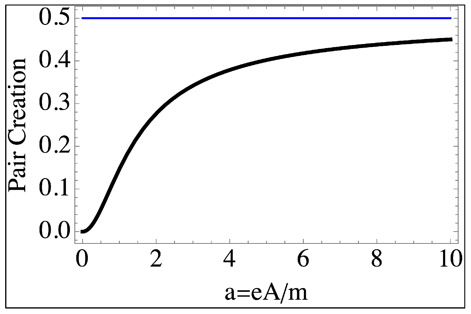
This result is illustrated in Figure 1. The maximum possible probability is $P_{max}=1/2$, and can only the attained asymptotically, for $a^2\to \infty$. As previously mentioned, this is a non-perturbative result, which is associated with an instantaneous electric field, created at $t=0$ by a potential discontinuity, represented by $\tau \to 0$ in Equation (6). In some sense, this is opposite to the Sauter-Schwinger process, which is associated with a constant electric field, which would correspond to $\tau \to \infty$ in the same equation.

We can see that, for $a^2\gg 1$, the probability for pair creation seems quite high, but this result has no immediate physical meaning, as it can be seen in the following. A possible way to produce a nearly instantaneous electric field is to use two counter-propagating laser pulses with a large amount of high-harmonic components, with frequencies $n\omega$ for $n=1,2,\dots ,N\gg 1$, and nearly constant amplitudes. Such laser pulses are currently created in the laboratory [12,13]. But, the field is never instantaneous, and, even for a very large but finite number N, a finite duration will persist. This will drastically reduce the above probability. Generalization of the present analysis to a finite duration field is discussed next.

4. Finite Time Scales

The general case of an arbitrary vector potential $\mathbf{A}\left(t\right)$ can be replaced by a sequence of infinitesimal temporal Klein processes. This sequence is described by a dynamical coupling between operators [25], as defined by

$$b_p\left(t\right)=B_p^{\prime }\left(t\right)d_p^{†}\left(t\right)exp\left[2i{\phi }_p\left(t\right)\right],d_p^{†}\left(t\right)=-B_p^{\prime }\left(t\right)b_p\left(t\right)exp\left[-2i{\phi }_p\left(t\right)\right],$$

(28)

where phase ${\phi }_p\left(t\right)={\int }^t{\omega }_p\left(t^{\prime }\right)d{t}^{\prime }$, and ${\omega }_p\left(t\right)=E\left(t\right)$ is the instantaneous particle energy corresponding to momentum $\mathbf{p}$. This is generalization of the discrete Bogoliubov transformations (14). Starting from Equation (16), we can easily get

$$B_p^{\prime }\left(t\right)=\sqrt{\alpha \left(t\right)}{\partial }_t\left(\frac{k}{E+m}\right),$$

(29)

where $k=[p_z-eA\left(t\right)]$ and $E=\sqrt{k^2+m^2}$, as before. This can also be written as

$$B_p^{\prime }\left(t\right)=\frac{1}{2E}\sqrt{2E(E+m)}\left[\frac{1}{E+m}-\frac{k^2}{E{(E+m)}^2}\right]{\partial }_{t}k.$$

(30)

Using ${\partial }_{t}k=-e{\partial }_{t}A=e\mathcal{E}\left(t\right)$, we finally get

$$B_p^{\prime }\left(t\right)=\frac{e\mathcal{E}\left(t\right)}{\sqrt{2E(E+m)}}\frac{m}{E}.$$

(31)

At this point, we should note that, for small $a=eA/m$, we can use $E\simeq m$, and we get the approximate expression

$$B_p^{\prime }\left(t\right)\simeq \frac{e\mathcal{E}\left(t\right)}{2E^2}m.$$

(32)

This agrees with Equation (24) of [18], if we reintroduce the transverse momentum, replacing m by $\sqrt{p_{\perp }^2+m^2}$. Solving the coupled Equation (28), for given initial conditions defined at $t=t_0$, we obtain

$$b_p\left(t\right)={\overline{A}}_p\left(t\right)b_p\left(t_0\right)+{\overline{B}}_p\left(t\right)d_p^{†}\left(t_0\right),d_p^{†}\left(t\right)={\overline{A}}_p\left(t\right)d_p^{†}\left(t_0\right)-{\overline{B}}_p\left(t\right)b_p\left(t_0\right),$$

(33)

with the new coefficients

$${\overline{A}}_p\left(t\right)=cos\left[r_p\left(t\right)\right],{\overline{B}}_p\left(t\right)=sin\left[r_p\left(t\right)\right].$$

(34)

Here, the squeezing parameter $r_p\left(t\right)$ is defined as

$$r_p\left(t\right)={\int }_{t_0}^t{B}_p^{\prime }\left(t^{\prime }\right)exp\left[2i{\phi }_p\left(t^{\prime }\right)\right]d{t}^{\prime },$$

(35)

and $B_p^{\prime }\left(t\right)$ is determined by Equation (31). Again, we find here the expected fermionic relation $|{\overline{A}}_p{\left(t\right)|}^2+{\left|{\overline{B}}_p\left(t\right)\right|}^2=1$, valid at all times. In order to proceed further, it is now convenient to rewrite Equation (31) as

$$B_p^{\prime }\left(t\right)=e\mathcal{E}\left(t\right)f\left(a\right),f\left(a\right)=\frac{m}{E}\frac{1}{\sqrt{k^2+{(E+m)}^2}}.$$

(36)

For particles created nearly at rest, we simply have $k^2\simeq a^2$ and $E=m\sqrt{1+a^2}$. We should also note that

$$k^2+{(E+m)}^2=m^2\left[a^2+{\left(1+\sqrt{1+a^2}\right)}^2\right].$$

(37)

In the exponential factor of Equation (35), we can use Equation (6), such that

$${\phi }_p\left(t\right)=m{\int }_{t_0}^t\sqrt{1+(a_0^2/4){\left[1+tanh(t^{\prime }/\tau )\right]}^2}d{t}^{\prime },$$

(38)

where we have used the normalized amplitude $a_0=eA/m$. Here, we have to assume that $t_0\ll -\tau$. Let us focus on the case of a large field amplitude, such that $a_0^2\gg 1$. In this case, the potential term will dominate over the mass term in most of the region $|t/\tau |\ll 1$. We can then use the approximation: $tanh(t/\tau )\simeq (t/\tau )$, and write

$${\phi }_p\left(t\right)=m{\int }_{-\tau }^t\sqrt{1+(a_0^2/4){\left[1+(t^{\prime }/\tau )\right]}^2}d{t}^{\prime },$$

(39)

Introducing the normalized imaginary time $\eta =-i{a}_0(1+t/\tau )/2$, we get

$$exp\left[2i{\phi }_p\left(t\right)\right]=exp\left\{-4\frac{m}{a_0}\left({\int }_0^1\sqrt{1-{\eta }^2}d\eta \right)+i{\varphi }_p\left(t\right)\right\},$$

(40)

where ${\varphi }_p\left(t\right)$ represents an oscillatory phase given by

$${\varphi }_p\left(t\right)=2m\tau {\int }_{t^{*}}^t\sqrt{1+(a_0^2/4){\left[1+(t^{\prime }/\tau )\right]}^2}d{t}^{\prime },$$

(41)

with $t^{*}=(2/a_0-1)\tau$. Noting that ${\int }_0^1\sqrt{1-{\eta }^2}d\eta =\pi /4$, we get the approximate expression

$$exp\left[2i{\phi }_p\left(t\right)\right]\simeq exp\left[-\pi \frac{m\tau }{a_0}\right]=\left[-\frac{\pi }{2}\frac{{\mathcal{E}}_c}{{\mathcal{E}}_0}\right].$$

(42)

Here, we have used the electric field amplitude ${\mathcal{E}}_0=m{a}_0/2e\tau$, which is the electric field applied during the interval $\Delta t=2\tau$, and introduced the critical field ${\mathcal{E}}_c=m^2/e$. In this exponential factor, we recognize the well-known Schwinger result. The oscillatory phase ${\varphi }_p\left(t\right)$ is also proportional to the ratio ${\mathcal{E}}_c/{\mathcal{E}}_0$, and for this reason contributes little to the final value of the squeezing factor $r\left(t\right)$. For simplicity, it will be ignored. We are now able to estimate the probability for particle-pair creation after a potential discontinuity with duration $2\tau$, as

$$P_p(t\ge \tau )={\left|{\overline{B}}_p\left(t\right)\right|}^2={sin}^2\left[r_p\left(t\right)\right|].$$

(43)

For small values of $|r_p\left(t\right)|\ll 1$, we simply get

$$P_p(t\ge \tau )\simeq F_p{\left(a_0\right)}^{2}exp\left[-\pi \frac{{\mathcal{E}}_c}{\mathcal{E}}\right],$$

(44)

with the auxiliary function

$$F_p\left(a_0\right)=\frac{1}{2}{\int }_{-a_0}^{a_0}\frac{dy}{\sqrt{1+y^2}{\left[y^2+{\left(1+\sqrt{1+y^2}\right)}^2\right]}^{1/2}},$$

(45)

where $a_0=2\tau e{\mathcal{E}}_0/m$, and the variable of integration is $y=a_{0}t/\tau$. This shows that the temporal Klein model with a finite temporal time-scale leads to a result that is similar to the previous discrete model of Section 3, but multiplied by the Schwinger exponential factor.

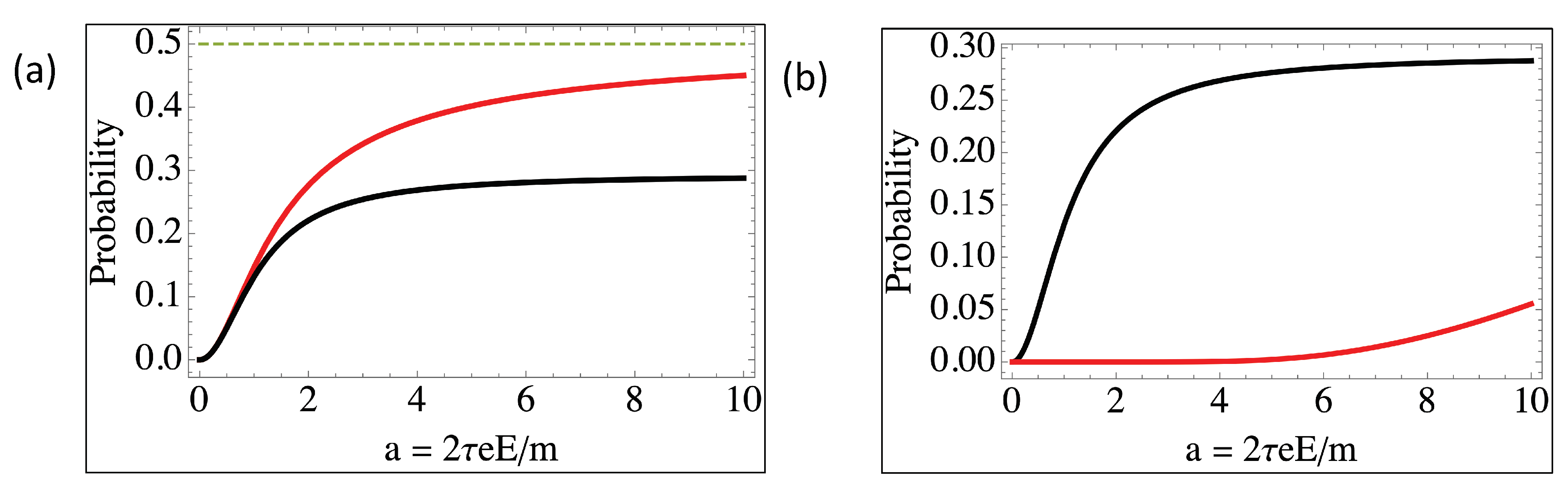
Detailed numerical comparison of the first factor in the probability of Equation (44) shows that the discrete model is valid in the region $a_0^2\le 1$, where $F_p{\left(a_0\right)}^2\simeq P_p\left(1\right)$, as given by Equation (27), but starts to diverge significantly in the region, $a_0^2\gg 1$. In particular, it tends to $P_p\left(1\right)/2$ in the limit of extremely large fields $a_0^2\to \infty$, as illustrated in Figure 2a. On the other hand, the influence of the exponential factor in Equation (44) is critical to the overall probability (see Figure 2b). This exponential factor is always dominant and drastically reduces the total probability, except in the extreme case of an infinitely sharp discontinuity, when $\tau \to 0$. Our approach is, therefore, able to establish a clear link between the temporal Klein model, describing electric fields with an infinitesimal duration, and the Schwinger model corresponding to electric fields with an infinite duration.

Although we have focused on the potential discontinuity with a tangent hyperbolic temporal shape, as dictated by Equation (6), the squeezing parameter $r_p\left(t\right)$ and the probability $P_p(t\ge \tau )$, given by Equations (35) and (43), stay valid for generic temporal field variations. We could, in particular, apply them to the case of periodically oscillating fields. For an arbitrary temporal variation, Equation (43) can be replaced by

$$P_p\left(t\right)\simeq {\left|{\int }_{t_0}^{t}d{t}^{\prime }\int d\omega F_p\left(\omega \right)exp\left[-i\omega t^{\prime }+2i{\phi }_p\left(t^{\prime }\right)\right]\right|}^2,$$

(46)

where $F_p\left(\omega \right)$ is the Fourier transform of the function $F_p\left(t\right)=e\mathcal{E}\left(t\right)f\left(a\right)$. The dominant contributions will correspond to $\omega \simeq 2m$. For a standing wave configuration with frequency ${\omega }_0$, which satisfies the vacuum momentum conservation, this would lead to ${\omega }_0\simeq 2m$, as expected. But, for large values of the oscillation amplitude $a_0$, the intrinsic nonlinear character of the function $f\left(a\right)$ will determine multiphoton pair creation processes, such that $n{\omega }_0\simeq 2m$, with integer $n\gg 1$. But this is outside the scope of the present work.

5. Conclusions

In this work, we have explored the temporal Klein model, associated with a sharp discontinuity of the electromagnetic vector potential. This model could be relevant to experiments using ultra-short electric field spikes in vacuum, as those created by intense laser pulses with a very high-harmonic spectral content.

We have considered the quantized fermionic field described by the Dirac equation, and we have focused on the influence of a finite temporal duration of the electric field spikes. Using this approach, we were able to derive general expressions for the probability for electron-positron pair creation in vacuum. This allowed us to establish a clear connection between two important models, that of a sharp discontinuity of the vector potential with negligible duration, and that of a constant electric field with infinite duration. This connection confirms the relevance of the Schwinger result for fields with a finite duration and, at the same time, is able to determine its limits.

The present results could also be used to study arbitrary oscillating fields, as briefly discussed, and to establish appropriate source terms for particle kinetic equations. But considerable work has already been done in that direction [18,19,20,21], and, for this reason, we have focused on the temporal Klein model. Finally, we note that our analysis assumes uniform potentials. An extension to space and time varying potentials is also possible, in a way similar to that used in Reference [22]. These problems will eventually be explored in a future publication.

References

- Klein, O. Die Reflexion von Elektronen an einem Potentialsprung nach der relativistischen Dynamik von Dirac. Z. Phys. 1929, 53, 157–165. [Google Scholar] [CrossRef]
- Dombey, N.; Calogeracos, A. Seventy Years of the Klein paradox. Phys. Rep. 1999, 315, 41–58. [Google Scholar] [CrossRef]
- Krekora, P.; Su, Q.; Grobe, R. Klein Paradox in Spatial and Temporal Resolution. Phys. Rev. Lett. 2004, 92, 040406. [Google Scholar] [CrossRef]
- Umul, Y.Z. A Survey on Klein Paradox. Optik 2019, 181, 258–263. [Google Scholar] [CrossRef]
- Katsnelson, M.I.; Novoselov, K.S.; Geim, A.K. Chiral Tunnelling and the Klein Paradox in Graphene. Nat. Phys. 2006, 2, 620–625. [Google Scholar] [CrossRef] [Green Version]
- Mendonça, J.T.; Guerreiro, A.; Martins, A.M. Quantum Theory of Time Refraction. Phys. Rev. A 2000, 62, 033805. [Google Scholar] [CrossRef]
- Mendonça, J.T.; Martins, A.M.; Guerreiro, A. Temporal Beam Splitter and Temporal Interference. Phys. Rev. A 2003, 68, 043801. [Google Scholar] [CrossRef]
- DiPiazza, A.; Muller, C.; Hatsagortsyan, K.Z.; Keitel, C.H. Extremely high-intensity laser interactions with fundamental quantum systems. Rev. Mod. Phys. 2012, 84, 20121177. [Google Scholar]
- Marklund, M.; Shukla, P.K. Nonlinear collective effects in photon-photon and photon-plasma interactions. Rev. Mod. Phys. 2006, 78, 591–640. [Google Scholar] [CrossRef] [Green Version]
- Ehlotzky, F.; Krajewska, K.; Zamiński, J.Z. Fundamental processes in quantum electrodymics in lasers fields of relativistic power. Rep. Prog. Phys. 2009, 72, 046401. [Google Scholar] [CrossRef]
- Gu, Y.-J.; Jirka, M.; Klimo, O.; Weber, S. Gamma Photons and Electron-Positron Pairs from Ultra-Intense Laser-Matter Interaction: A Comparative Study of Proposed Configurations. Matter Radiat. Extrem. 2019, 4, 064403. [Google Scholar] [CrossRef] [Green Version]
- Paul, P.M.; Toma, E.S.; Breger, P.; Mullot, G.; Augé, F.; Balcou, P.; Muller, H.G.; Agostini, P. Observation of a Train of Attosecond Pulses from Hugh Harmonic Generation. Science 2001, 292, 1689–1692. [Google Scholar] [CrossRef]
- Vincenti, H.; Quéré, F. Attosecond Lighthouses: How to Use Spatiotemporally Coupled Light Fieds to Generate Isolated Attosecond Pulses. Phys. Rev. Lett. 2012, 108, 113904. [Google Scholar] [CrossRef] [PubMed] [Green Version]
- Mendonça, J.T. Superradiance in Quantum Vacuum. Quantum Rep. 2021, 3, 3. [Google Scholar] [CrossRef]
- Schwinger, J. On gauge invariance and vacuum polarization. Phys. Rev. 1951, 82, 664–679. [Google Scholar] [CrossRef]
- Itzykson, C.; Zuber, J.-B. Quantum Field Theory; McGraw-Hill: New York, NY, USA, 1980. [Google Scholar]
- Brezin, E.; Itzykson, C. Pair Production in Vacuum by an Alternating Field. Phys. Rev. D 1970, 2, 1191–1199. [Google Scholar] [CrossRef]
- Schmidt, S.; Blaschke, D.; Röpke, G.; Smolyansky, S.A.; Prozorkevich, A.V.; Toneev, V.D. A Quantum Kinetic Equation for Particle Production in the Schwinger Mechanism. Int. J. Mod. Phys. E 1998, 7, 709–722. [Google Scholar] [CrossRef] [Green Version]
- Tanji, N. Dynamical View of Pair Creation in Uniform Electric and Magnetic Fields. Annals Phys. 2009, 324, 1691–1736. [Google Scholar] [CrossRef] [Green Version]
- Bell, A.R.; Kirk, J.G. Possibility of Prolific Pair Production with High-Power Lasers. Phys. Rev. Lett. 2008, 101, 200403. [Google Scholar] [CrossRef] [Green Version]
- Deffner, S. Shortcuts to Adiabaticity: Suppression of Pair Production in Driven Dirac Dynamics. New J. Phys. 2016, 18, 012001. [Google Scholar] [CrossRef]
- Aleksandrov, I.A.; Kohlfürst, C. Pair Production in Temporally and Spatially Oscillating Fields. Phys. Rev. D 2020, 101, 096009. [Google Scholar] [CrossRef]
- Umesawa, H. Advance Field Theory; American Institute of Physics: New York, NY, USA, 1993. [Google Scholar]
- Bicudo, P.; Ribeiro, J.E. Current.Quark Model in a 3P0 Condensed Vacuum. Phys. Rev. D 1990, 42, 1611–1624. [Google Scholar] [CrossRef] [PubMed]
- Mendonça, J.T.; Guerreiro, A. Time Refraction and the Quantum Properties of Vacuum. Phys. Rev. A 2005, 72, 063805. [Google Scholar] [CrossRef]
Figure 1.
Probability for particle pair creation by a potential discontinuity at time , with normalized amplitude (black curve). For reference, the maximum probability, , is also shown (in blue).
Publisher’s Note: MDPI stays neutral with regard to jurisdictional claims in published maps and institutional affiliations. |
© 2021 by the author. Licensee MDPI, Basel, Switzerland. This article is an open access article distributed under the terms and conditions of the Creative Commons Attribution (CC BY) license (https://creativecommons.org/licenses/by/4.0/).
Share and Cite
MDPI and ACS Style
Mendonça, J.T. Temporal Klein Model for Particle-Pair Creation. Symmetry 2021, 13, 1361. https://doi.org/10.3390/sym13081361
AMA Style
Mendonça JT. Temporal Klein Model for Particle-Pair Creation. Symmetry. 2021; 13(8):1361. https://doi.org/10.3390/sym13081361
Chicago/Turabian StyleMendonça, José Tito. 2021. "Temporal Klein Model for Particle-Pair Creation" Symmetry 13, no. 8: 1361. https://doi.org/10.3390/sym13081361
Note that from the first issue of 2016, this journal uses article numbers instead of page numbers. See further details here.