
Effects of Probability-Distributed Losses on Flood Estimates Using Event-Based Rainfall-Runoff Models

School of Engineering, Design & Built Environment, Western Sydney University, Locked Bag 1797, Penrith, NSW 2751, Australia
*
Author to whom correspondence should be addressed.
Water 2021, 13(15), 2049; https://doi.org/10.3390/w13152049
Submission received: 21 June 2021
/
Revised: 16 July 2021
/
Accepted: 23 July 2021
/
Published: 27 July 2021
(This article belongs to the Special Issue Rainwater and Stormwater Harvesting for Sustainable Water Cycle Management)
Abstract
:Probability distributions of initial losses are investigated using a large dataset of catchments throughout Australia. The variability in design flood estimates caused by probability-distributed initial losses and associated uncertainties are investigated. Based on historic data sets in Australia, the Gamma and Beta distributions are found to be suitable for describing initial loss data. It has also been found that the central tendency of probability-distributed initial loss is more important in design flood estimation than the form of the probability density function. Findings from this study have notable implications on the regionalization of initial loss data, which is required for the application of Monte Carlo methods for design flood estimation in ungauged catchments.
1. Introduction
In rainfall-runoff modeling, loss parameter is one of the most important parameters, which refers to amount of rainfall that does not appear at the stream directly, which mainly consists of infiltration, evapotranspiration, interception, depression storage, and transmission losses. Several loss models have been proposed for use with event-based rainfall-runoff models, such as the initial loss-continuing loss (IL-CL) model, the Soil Conservation Service (SCS) Curve Number model and probability-distributed model (PDM) [1]. More sophisticated loss models exist that can simulate evaporation and movement of water within the soil profile and in the groundwater layers, such as the Xinanjiang model [2] and soil moisture accounting model [3]. In many cases however (particularly in poorly gauged catchments), the simplest loss models such as IL-CL model can produce reasonably accurate design flood estimates. However, a key limitation of event-based loss models is the lack of knowledge about the antecedent moisture condition of the catchment [4,5]. Given the importance of antecedent moisture conditions in flood estimation [6], several methods have been suggested to overcome this limitation [7,8,9,10,11]. In addition, joint probability approaches [12] are often used to incorporate the natural variability of antecedent moisture conditions in a catchment. This has been considered in several studies based on various loss models including the SCS Curve Number method [8,13,14], PDM [15] and the Green–Ampt infiltration equation [16]. Stochastic loss modeling is becoming popular in rainfall-runoff modeling to account for its inherent variability [17,18,19]. Here losses are assumed to be a random variable and is generally specified by a probability distribution.
In many Australian catchments, simplistic loss models are often found to provide reasonable approximations of runoff generation; with the lumped conceptual IL-CL model being widely adopted [20,21]. The initial loss is based on the antecedent moisture prior to an event and is specifically defined as the amount of rainfall occurring before the effective start of runoff. In calculating initial loss, a surface runoff threshold value (such as 0.01 mm/h) is generally used following the approach of Rahman et al. [12] where it is assumed that surface runoff starts when this surface runoff threshold is exceeded. The initial loss can be estimated by examining the continuous rainfall and runoff data of the given catchment. The continuing loss is a combination of other losses but is mostly based on the infiltration rate across the catchment and is defined as a ‘constant loss rate’ throughout the remainder of the storm under consideration. Continuing losses are dependent on catchment characteristics and is generally considered to be a ‘fixed input’ in a given catchment, except for changes over time due to change of catchment soil profile, plantation, and other similar factors. Although variability in the continuing loss has been studied in the past [22], this variability is most likely due to uncertainties (both epistemic and aleatoric) and not the inherent random nature of the parameter itself. In contrast, the initial loss is a measure of the antecedent catchment wetness of a given storm event. Given the stochastic nature of meteorological factors involved, primarily wetting and drying processes, initial loss should ideally be treated as a random variable in rainfall-runoff modeling. In the use of Monte Carlo simulation methods, the joint probabilities of key inputs, such as initial loss, are needed for rainfall-runoff modeling [12,17].
Due to complex spatial and temporal variability of hydro-meteorological processes, losses cannot be measured in field studies very accurately rather it needs to be estimated from calibration of historic rainfall-runoff records. Historic records (such as streamflow and rainfall), however, are limited in many countries, including Australia. Data are further limited using only the most extreme rainfall-runoff events in rainfall-runoff modeling (rather than records in their entirety) and gauge recording issues (such as rating curve extrapolation) during these extreme events. These data limitations make it difficult to identify the underlying probability distribution for initial loss. There have been few studies that have examined the stochastic nature of initial loss and identified suitable initial loss probability distributions with a reasonable degree of accuracy, as noted below.
Regionalization of losses is needed to apply rainfall-runoff models for ungauged catchments. Regionalization refers to characterization of regional behavior of a variable of interest (such as flood quantile or parameters of a probability distribution) over a given region so that the variable can be estimated at any arbitrary ungauged location within the study area. One of the most common regionalization approaches is regional flood frequency analysis (RFFA) where a prediction equation is developed for a flood quantile (e.g., 100-year flood) or for parameters of a probability distribution as a function of climatic and catchment characteristics [23,24,25,26]. The regionalization of initial loss refers to identification of the regional mean or median initial loss value (in simplistic form) or regional values of a probability distribution function that can specify regional initial loss values.
Rahman et al. [12] examined the sensitivities of design flood estimates to uncertainties in the initial loss distributions. The authors found the Beta distribution to be a reasonable fit with respect to descriptive statistics of the observed and simulated initial loss data. However, the authors did not apply any goodness-of-fit tests in selecting an appropriate probability distribution for initial loss. Design flood estimates were found to be most sensitive to the variance and upper limits when specifying model parameters. The study by Rahman et al. [12] was limited to ten catchments in a relatively mild climatic region of Victoria, Australia, therefore, Tularam and Ilahee [22] extended the analysis to 15 catchments in tropical Queensland. The Beta distribution originally suggested by Rahman et al. [12] for Victorian catchments was found be appropriate for the initial loss data in tropical Queensland.
Previous studies [12,22] adopted crude goodness-of-fit tests, which are problematic as parameters were estimated from the same dataset that the model fit was derived. Gamage et al. [27] overcame this limitation by adopting a more robust method of distributional model fitting. In this regard, Gamage et al. [27] were able to assess the probability density model most suited to the true (unknown) initial loss distribution and for the six South Australian catchments, the Gamma distribution was found to reasonably represent initial loss data. Several other Australian studies have also derived and applied initial loss distributions within a Monte Carlo simulation framework [17,28,29,30]; each study found either the Beta or Gamma distributions to be the most representative of the true underlying distribution for initial loss.
The principal objective of the paper is to identify a probability distribution that is better suited to represent the initial loss data for a range of catchment and climatic characteristics in Australia. The probability-distributed losses are becoming more common in Australian applications as Australian Rainfall and Runoff has recommended Monte Carlo simulation in rainfall and runoff modeling [20,31]. In this regard, five probability distributions (four parametric and one nonparametric model) are assessed using a bootstrap-based goodness-of-fit method, given three distance measures based on the empirical density function (EDF). Secondly, the impact of the relative accuracy of parameters of the underlying initial loss distributions on design flood estimates is evaluated. Given the lack of knowledge regarding the true underlying distribution, different functional forms are examined along with possible errors in the descriptive statistics (mean and variance) of the initial loss data. The investigation is then extended to the effect of regionalization of model parameters and distributions to evaluate the impact of uncertainties in initial losses on design flood estimates.
2. Bootstrap-Based Goodness-of-Fit Procedure
2.1. Probability Distributions
Previous studies commonly found the Gamma and Beta distributions to be representative of the initial loss data in Australia. Both distributions were included in this study, along with the Normal and Weibull distributions for comparative purposes. Parameters of a probability distribution can be estimated from an observed sample using several techniques, both numerical and graphical, which produce notably different parameter estimates and confidence limits. More commonly used techniques for estimating distributional parameters include the method of moments (MOM), method of maximum likelihood (ML) and probability weighted moments. In this study, the distributional parameters are estimated using the ML method, which maximizes the conditional probability of generating the observed data to select the parameters.
These parametric distributions rely on the assumption that the population (which the observed data sample belongs to) has an underlying parent distribution. This results in the observed data being fitted to a probability density function with a known theoretical distribution. Nonparametric approaches, however, make no prior assumption about the form of the underlying probability distribution. This method, however, relies heavily on the observed data and its empirical grouping into bins. This study, therefore, compared both parametric and nonparametric distributions for describing initial losses. The most widely used nonparametric method is the kernel density estimate (KDE) [32].
For a given data sample and kernel function , the probability density can be estimated by:
where is a smoothing factor known as the bandwidth and is the Gaussian kernel, specified as
The bandwidth is the most important characteristic of a KDE, with a strong influence on the shape of the density function. It is, therefore, necessary to implement a reliable method to estimate the optimal bandwidth [33,34,35]. The optimal bandwidth can be estimated using the so-called rule of thumb methods [36], as in Equation (2), which is based on minimizing the asymptotic mean squared error (AMISE) for a kernel density estimate.
where is the inter-quartile range and is the sample standard deviation. Jones et al. [37] found the estimator to be “close enough to be reasonably representative” as compared to the best estimate.
2.2. Model Selection
The model selection methods are used to infer the model that best fits the observed data. These are commonly measures of distance between the parent and hypothetical distributions. Three of the most commonly used goodness-of-fit tests based on the EDF are adopted in this study. Each of these may be defined regarding the corresponding order statistics (for brevity ), as follows:
- Kolmogorov Smirnov (K-S) test statistic:
- Cramér–von Mises (C–vM) test statistic:
- Anderson-Darling (A-D) test statistic:
These classical methods, however, estimate the parameters and fit the model to the available dataset, leading to the failure of such techniques in many cases [38]. Bootstrap resampling techniques [39,40] overcome these limitations and have been shown to be effective in wide range of scenarios [41].
The bootstrap resampling technique adopted here is the parametric bootstrap, which undertakes Monte Carlo simulations from a parametric model of the data. This procedure allows for more reliable critical values to be derived (irrespective of parameter values), along with an approximation of the p-values. The procedure can be formalized as follows: For an observed dataset from unknown distribution , the most suited hypothetical distribution can be assessed for each probability distribution:
- Estimate the model parameters () from and construct the cumulative density function (CDF)
- Evaluate , and (Equations (4)–(6)), where
- Generate bootstrap samples of size from , denoted as given
- Estimate from and construct the CDF
- Evaluate , and (Equations (1)–(3)), where
For a given test statistic (), the critical value is the empirical quantile of order of . The p-value can also be approximated as . The null hypothesis ( versus ) can be rejected if , and for comparative purposes if . Given the hypothetical models (being the Gamma, Beta, Weibull, Normal or KDE models) where the null hypothesis is not rejected, the most suited distribution for the observed data is the model with the smallest test statistic , indicating the model closest to .
It should be noted here that the study area (eastern NSW) was considered to be a homogeneous region to regionalize the distribution of initial loss. The classical homogeneity test, such as Hosking and Wallis [42] was not applied as our objective was to regionalize the parameters of the assumed probability distributions for the initial loss. However, three goodness-of-fit tests were applied to assess whether the hypothesized distribution adequately fits the observed initial loss data as discussed above.
3. Rainfall-Runoff Modeling
The principal focus of this study is to evaluate the effect of probability-distributed initial losses on design flood estimates when used within a Monte Carlo simulation framework. The nature of Monte Carlo framework is the incorporation of an expected degree of variability into the process/system. To assess the variability in initial loss data alone, while still allowing for a Monte Carlo framework, random seeds for all other input variables of the rainfall-runoff model are kept fixed to allow for reproducible variability in each of these input variables.
3.1. Rainfall-Runoff Model
The rainfall-runoff model adopted in this study is a conceptual semi-distributed model called RORB [43]. It is an event-based model that is here run at an hourly time step. The catchment river system is represented in the model by a network of model storages. Runoff generation is modeled here using the initial loss-continuing loss model; however, the initial loss-proportional loss model is also available for use. In RORB, non-linear storage routing is used to transform direct runoff and simple river routing is employed where flows are simply lagged in time. This model is adopted due to its simplicity, which lends itself to fast computations (beneficial for large data sets), its flexibility, which allows for ease-of-use in joint probability approaches, and its ability to approximate catchment response [44].
Baseflow is not modeled in RORB therefore it was calculated externally using a recursive digital filter, which was later added to the surface runoff hydrograph. Input precipitation depth was estimated using intensity frequency duration (IFD) calculator (Australian Bureau of Meteorology). The areal average precipitation over the catchment was estimated using areal reduction factor based on the catchment area, burst duration and return period [45]. Catchments were spatially divided into several subareas and stream reaches to account for the spatial heterogeneity of catchment and rainfall characteristics. Precipitation was estimated as spatial averages for each subarea using natural neighbors interpolation based on several surrounding rainfall gauges. The temporal pattern data were obtained from Australian Rainfall and Runoff data hub [27].
3.2. Model Calibration
The calibration of each RORB model is undertaken using several observed rainfall-runoff events. Three model parameters are calibrated in this study: specifically, the routing parameter, and the initial loss and continuing loss for the runoff generation model. Calibration of the parameter set involved optimizing four key statistics; being the absolute differences in the peak flow, time to peak flow, and 72 h runoff volume representative of biases in magnitude, timing and mass respectively, and the average absolute ordinate error (being the average absolute error between modeled and gauged flows at each time step) representative of the overall shape of the flood hydrograph.
3.3. Stochastic Design Storms
A statistical storm approach, based on depth-duration-frequency (DDF) data, is employed in this study. In Australia, a revision of DDF data was completed in 2016 as part of Australian Rainfall and Runoff, which provides regionalized burst DDF data for a 0.025° resolution grid across Australia [31]. The data are provided for standard durations between 1 min and 168 h, ranging in frequency from 63.2% to 1% annual exceedance probability (AEP) (equal to return periods of 1 year to 100 years).
DDF data represents design rainfall at a point, therefore to estimate rainfall across an entire catchment, areal reduction factors are used to provide estimates of areal precipitation. Areal reduction factors have been calculated specifically for Australian conditions [45] and are therefore adopted in this study. Both short duration (less than 18 h) and long duration (equal to or longer than 18 h) values have been derived based on catchment area, rainfall duration, and rainfall frequency.
The temporal distribution of rainfall throughout the event needs to be specified. In Australia, storm temporal patterns from historic events have been regionalized as part of the revision of Australian Rainfall and Runoff [46]. These storm patterns are identified by their critical burst duration (being the duration of the rarest burst within the storm period), as opposed to the total storm duration. Recorded events are regionalized using a region-of-influence approach, based on the similarity of source event characteristics (original event from the source pluviograph) to target event characteristics (design event at the target location). Patterns are available for standard burst durations between 5 min and 168 h, and burst frequencies rarer than the 63.2% AEP (above a return period of 1 year). These regionalized historic temporal patterns allow for ensembles of patterns to be generated for each rainfall duration and frequency.
The DDF data discussed earlier is based on burst events (as in the rarest burst within a storm for a given duration); however, in this study we adopt a storm event approach. For this reason, design burst depths need to be transformed into design storm depths. Here, the design burst depth is transformed using the storm to burst rainfall ratio (being the ratio of the total depth to the critical burst depth for the specified historic temporal pattern) to scale the burst depth up to a storm depth. This method is limited in that the pre- and post-burst periods are assumed to scale at the same rate as the critical burst, while this assumption is reasonable in current conditions, it could prove problematic in climate change scenarios where bursts have been seen to scale faster.
3.4. Design Flood Estimation
A classical approach to design flood estimation first assumes the peak flow and causative rainfall are probability neutral (as in having equal AEPs). Second, several storm durations (around the time of concentration, considering the catchment size) are simulated, then the design flood becomes the hydrograph that produces the highest peak across all durations. One of the key limitations of this approach is the use of a single design storm and parameter set for each given duration. Here, this classical approach has been modified to incorporate the joint probability of key flood producing inputs using Monte Carlo simulation. Crude Monte Carlo sampling techniques are computationally expensive, therefore, to improve the efficiency of the Monte Carlo simulations a stratified sampling approach is adopted with 50 bins and 50 runs per bin.
The depth, frequency and temporal distribution of rainfall in the design storm event were treated as random variables (as outlined in Section 3.3). The initial loss was also treated as a random variable specified by a probability distribution. However, remaining inputs were fixed, including the burst rainfall duration of the design storm, spatial distribution of rainfall across the catchment, routing parameter for modeling catchment response and continuing loss for calculating rainfall excess. Rainfall was assumed to be spatially uniform across the catchment; this should have minimal impact given the relatively small catchment sizes and general homogeneity of design rainfall depths throughout each catchment.
The regional design floods at a given site were estimated by a RORB model where regional initial loss value (specified by a probability distribution) was adopted as the input value along with other regional/at-site input data). To assess the relative accuracy of the regional design flood estimates, these were compared with the observed design floods, which were estimated by an at-site flood frequency analysis assuming a GEV distribution. Here, the parameters of the GEV distribution were evaluated using the maximum likelihood estimation method.
To determine the impact of a single variable (the initial loss) within a Monte Carlo framework an entirely stochastic modeling approach cannot be adopted due to the inherent variability between Monte Carlo sets. A pseudo-random approach is therefore applied, where the random seed of each variable is specified to ensure predictability between Monte Carlo sets while accounting for the joint probability of key inputs.
4. Study Area and Data
4.1. Historic Data Sets
Previous Australian studies have evaluated the functional form of initial loss data based on specific geographic or climatic regions. Here we aim to derive probability-distributed initial losses for a wide range of catchments across Australia. In addition to studies exploring the form of initial loss data (as discussed earlier), many more studies required the calibration of initial loss data; for instance, prior to the use of joint probability approaches and sufficient computing power, several studies calibrated initial loss data to derive a single design initial loss estimate [47,48], rather than probability-distributed losses. More recently, Hill et al. [49] conducted an Australia-wide study of loss models, as part of a major revision of Australian guidelines on flood estimation (Australian Rainfall and Runoff). The objectives of the study were two-fold; first, the assessment of the most appropriate runoff generation model for Australian conditions, and secondly, the determination of probability-distributed loss values for recommendation throughout Australia. Based on an analysis of 38 small Australian catchments, the initial loss-continuing loss model was recommended with stochastic initial losses (based on the empirical distribution function).
Historic initial loss data sets were collated in this study to incorporate a wide range of geographic and meteorological conditions throughout Australia. Five Australian studies, with small to medium sized catchments, were selected due to their availability and coverage throughout Australia, as follows:
Although a total of 119 catchments were calibrated across the five studies, given some of these studies were not intended for deriving probability distribution of initial losses, several catchments contained sample sizes too small to derive the functional form from the data. Additionally, several catchments overlapped between studies. For this reason, individual catchments that contained a sample size less than ten or that were duplicated across studies were removed, leaving a total of 92 catchments throughout Australia for our study. A sample size of ten is still considered to be on the limit for deriving probability distributions; however, there is a balance between the sample size of the initial loss data and the total number of catchments that are included. For example, a total of 92 catchments were found to contain more than 10 events; however, when this number is increased to 30 events (considered to be appropriate for deriving probability distributions), only 24 catchments remain in four studies.
4.2. Study Catchments
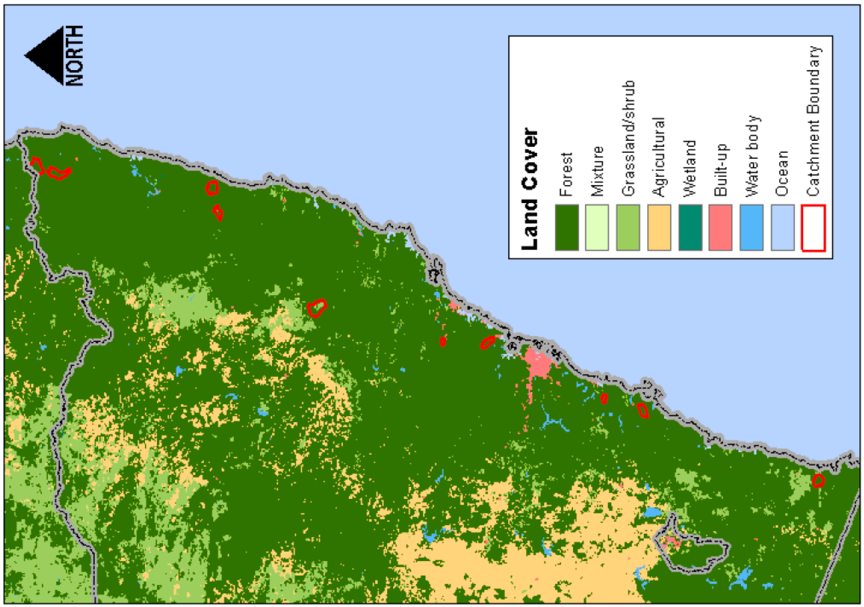
Further investigations into the impact of initial losses on design outputs are carried out for eight small to medium sized catchments (shown in Figure 1) along the east coast of New South Wales (NSW), in Australia. Table 1 lists key geographic and meteorological characteristics along with the volume of data used for model calibration (see Figure 2). Floods in this part of Australia are dominated by frontal rainfall events and convective storms. The selected catchments are rural (partially forested and agricultural), without any major upstream controls or built-up areas.
There is little variability in the land cover across the study catchments, with catchments being mostly forested and grassland. The mean annual rainfall for the centroid of each catchment is seen to vary from 802 to 1890 mm (with values listed for each catchment in Table 1), the values do not show any particular spatial trends from north to south. The mean annual runoff across the catchments shows greater variability with 52 to 1424 mm of runoff, resulting in annual runoff coefficients (being the mean annual rainfall divided by runoff) of between 0.065 and 0.776. Little climate variability was noted for these catchments according to the Köppen climate classification, with most catchments considered temperate with no dry season and mild, mid to hot summers.
5. Results
In this section, first the probability distribution better suited to initial loss data from several historic studies is presented. Thereafter, the variability of peak flow estimates caused due to the differences of initial loss probability distributions where uncertainties exist is investigated; specifically, the impact of assuming a probability density function, uncertainties in the descriptive statistics of observed datasets and unknowns when regionalizing distributions of initial losses are discussed.
5.1. Probability-Distributed Initial Losses
The first objective was to evaluate the functional form of initial losses for a wide range of catchments throughout Australia. For this purpose, a bootstrap-based goodness-of-fit procedure was employed, as explained in Section 2, using previously calibrated initial loss data sets, according to Section 4.1. The null hypothesis was evaluated for all 92 catchments and five probability distributions, using three goodness-of-fit tests at a significance level 10%. It should be noted that 5% or 1% significance levels can also be adopted; however, use of 10% level is commonly accepted in statistical hydrology [12,27]. The quality of the goodness-of-fit test statistics is dependent on the unknown underlying distribution, on the distribution parameters and on the sample size. Although these tests can be quite powerful in some situations, they may produce erroneous statistics in others. With this in mind, here we will highlight some of the more interesting findings that can be drawn from the bootstrap procedure.
The three goodness-of-fit tests are separately applied to each of the catchment data sets and a count of the number of catchments in which the null hypothesis is not rejected is reported for each study (see Figure 1). The first interesting result is that the goodness-of-fit tests appear to be of similar magnitudes, except for the A-D test for the Weibull distribution. Apart from this one anomaly, we cannot reject the fit to the remaining candidate distributions for a large proportion (typically more than half) of the 92 study catchments. In particular, it is noted that most catchments could not be rejected when using the Beta and KDE distributions. However, this is to be expected given that both distributions have the largest parameter sets. Application of the Weibull distribution at this point, appears to be questionable for the initial loss data.
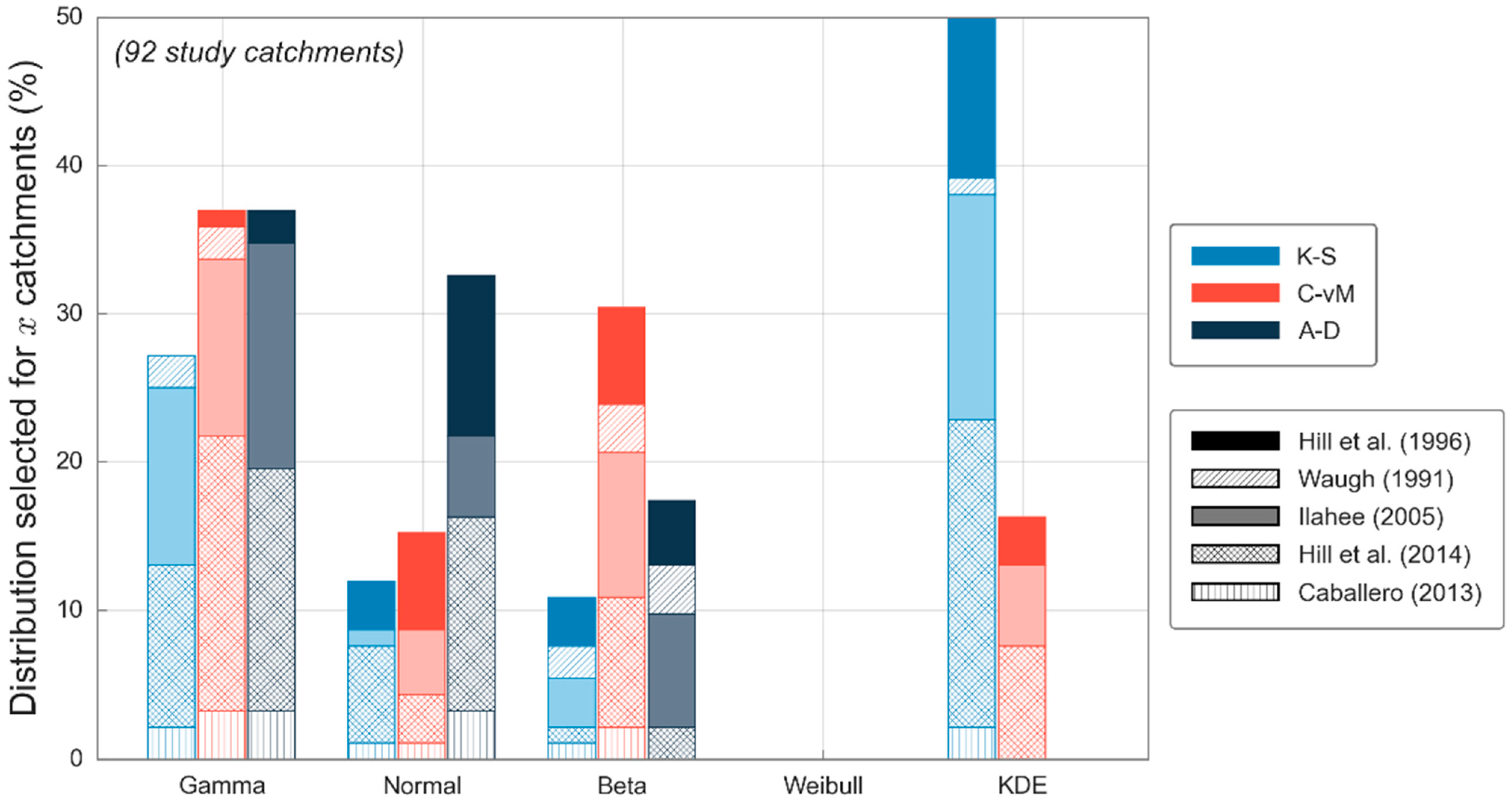
Following on from this, the percentage of cases for which each candidate distribution is selected as the most representative distribution (see Section 2.2) for each goodness-of-fit test is reported for each study (see Figure 3). Here it can be seen that three candidate distributions (Gamma, Normal and Beta) were selected for a rather large percentage of catchments across all three goodness-of-fit tests, which demonstrates their potential suitability for representing the underlying initial loss distribution. The KDE distribution; however, returned mixed results across the three goodness-of-fit tests, with the distribution not being selected at all using the A-D test, but then being selected for 50% of catchments using the K-S test.
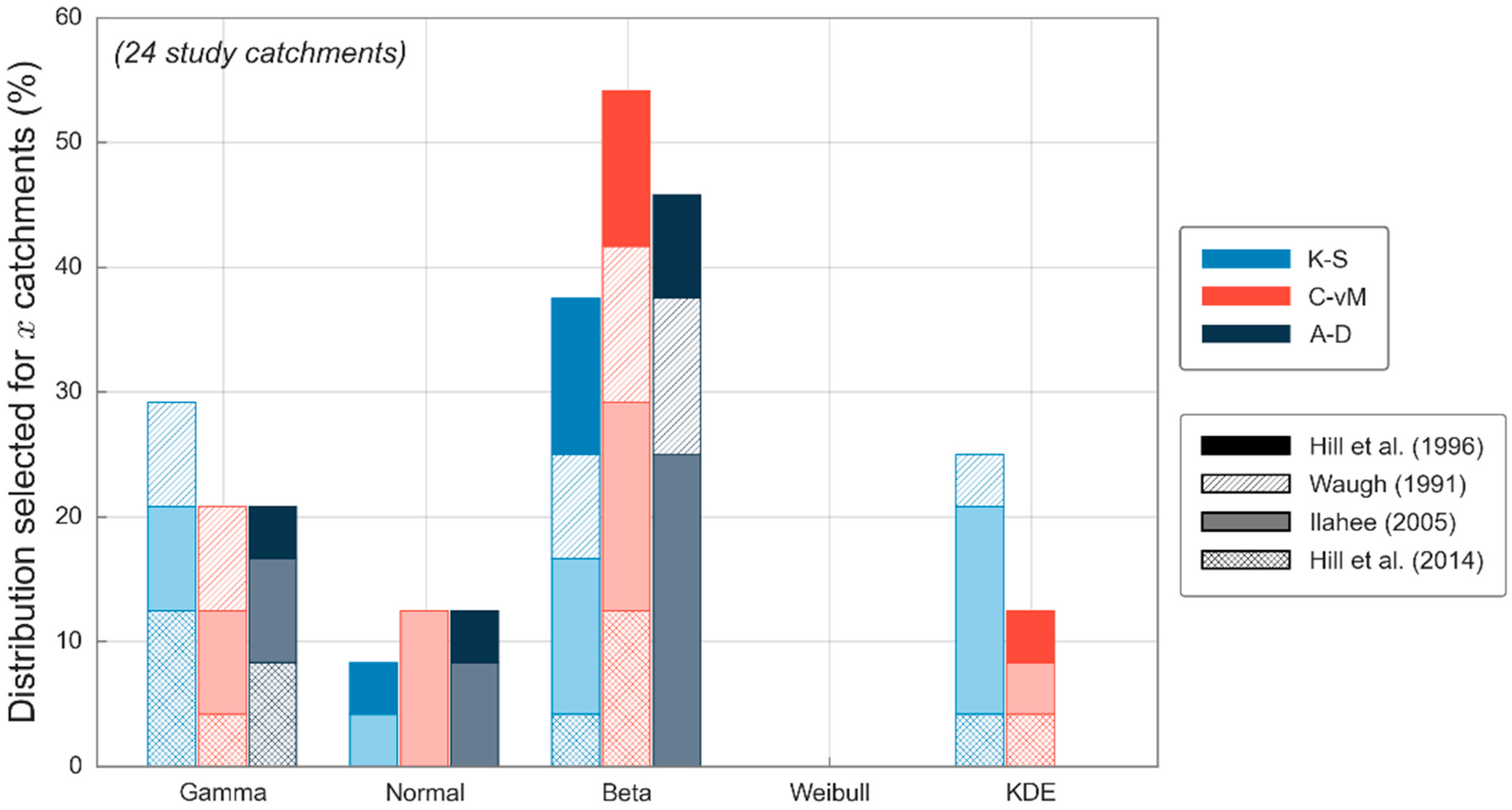
It was stated earlier that while not ideal, sample sizes of ten or more were included in this analysis. Realistically, a sample size of 25 to 30 is required to accurately derive probability distributions, any less than this could result in overfitting of the data. For this reason, a comparison of results using sample sizes greater than 10 and 30 was employed. A total of 24 study catchments were found to have sample sizes above 30 across four studies, resulting in less variability in geographic and meteorological characteristics. The number of catchments in which the null hypothesis is not rejected (see Figure 2) remained relatively similar using the two sample size thresholds (in terms of percentages). However, results from the selection of a single distribution that better fits the observed data changed markedly (see Figure 3 for a threshold of ten and see Figure 4 for a threshold of 30). Similar biases are noted for the KDE distribution; however, where the smaller threshold resulted in similar results across the Gamma, Normal, and Beta distributions, a larger threshold results in the Beta distribution becoming dominant. The Gamma and Normal distributions are still selected as better fit for rather large percentages but are relatively small in comparison to the Beta distribution.
Although none of the distributions can be universally chosen as the best, some recommendations can still be made. Among the five distributions, the Beta and Gamma distributions are considered most suitable for rainfall-runoff modeling within a Monte Carlo environment.
5.2. Effect of Functional Form of Initial Losses on Flood Estimates
After the initial selection of probability distributions most suited to flood modeling, design floods are estimated (as described in Section 3) using all five candidate distributions successively for the eight study catchments (outlined in Section 4.2). Each candidate distribution is used to model the calibrated initial loss data for each catchment (sample sizes listed in Table 1), with parameters estimated using the MLE method. Design flood estimates resulting from each successive candidate distribution are compared using relative errors of the peak flows:
where Q is the recorded/actual peak flow and is the predicted peak flow. Here the simulated peak flow represents the results from each successive candidate distribution and given the actual peak flow is unknown, here it is taken as the average value across all candidate distributions:
where i the ith candidate initial loss distribution given {i = 1, ⋯, m}.
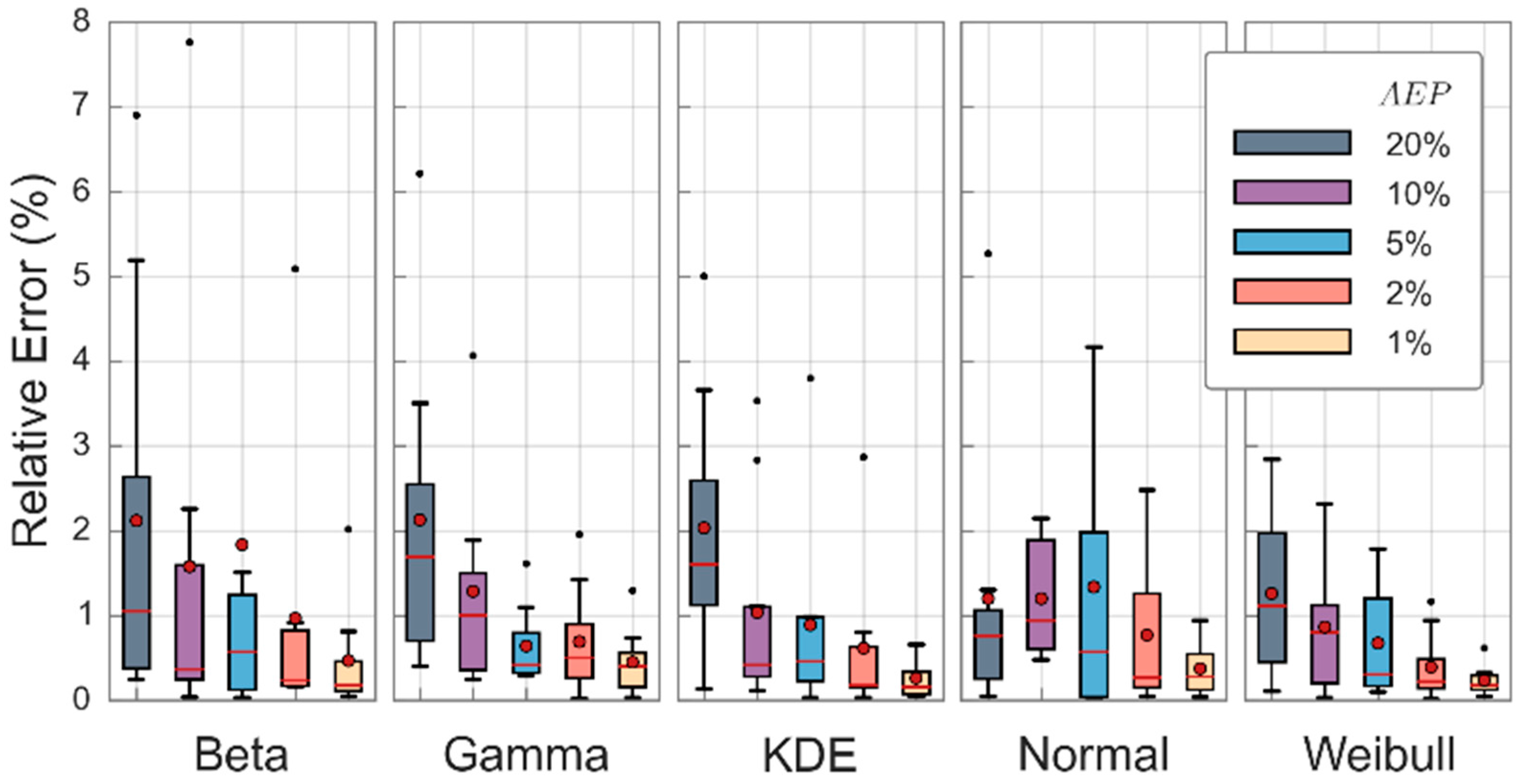
The results are shown as boxplots, which demonstrate the relative errors across the eight study catchments for each of the five quantiles and candidate distributions (see Figure 5); where the boxes represent the IQR, the red horizontal line signifies the median value, and the red circle marker indicates the mean value. Please note that the more frequent events tend to result in greater variability; this phenomenon is expected as initial losses represent a much greater proportion of total rainfall depths in frequent events as compared to rare events. The main result here is the similarity of design floods resulting from different candidate distributions, with most peak flows only deviating from the mean by about ±3%.
5.3. Effect of Statistical Uncertainties in Initial Losses on Flood Estimates
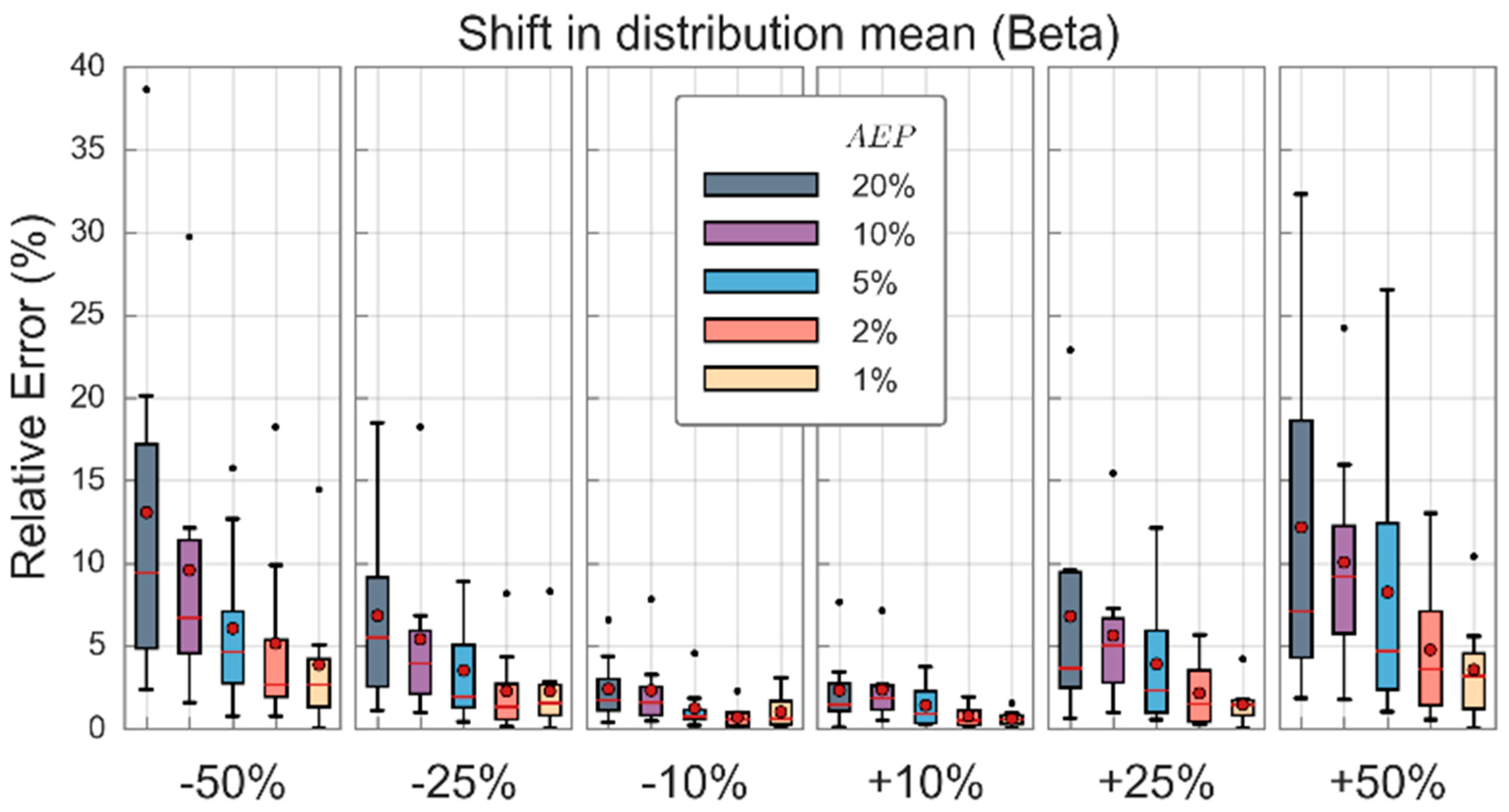
Distribution assumptions as we have discovered have little impact on design floods; however, issues may also arise from uncertainties in the sample dataset due to limited sample sizes, measurement uncertainty of data used in calibration and model structural uncertainty, among others. Here design floods are estimated using six shifted distributions for the eight study catchments; the distribution is shifted by ±10%, ±25% and ±50% of the mean value in each succession. Relative errors of the design floods are calculated according to Equation (7), where the actual peak flow is taken to be the design floods resulting from the original candidate distribution and the predicted peak flow is the design flood estimated using the shifted distributions.
Design floods using shifted distributions were estimated for all five candidate distributions; however, given the similarity in results between distributions only the results for the Beta distribution is presented (see Figure 6). Uncertainties in the mean initial loss value tended to result in less than two fifths of the uncertainty in design floods; i.e., peak flow estimates were within ±4% of actual peak flows when the mean initial loss shifted by ±10%, similarly peak flow errors were within ±10% and 20% when the mean shifted by ±25% and ±50%, respectively. Uncertainties of up to 10% in the mean initial loss value have negligible effect on design flood estimates. Similarly, for applications where events rarer than the 1% AEP are of interest, uncertainties of up to 50% in the mean value have minor impacts on design flood estimates. Additionally, of interest, for applications where events rarer than the 1% AEP are of interest, the mean initial loss value has minimal effect on design floods for up to ±50% uncertainty in mean values.
Similarly, the variance of each candidate distribution was varied to determine the significance of the distribution tails on peak flow estimates. The variance of each distribution was altered by ±10%, ±25% and ±50% while keeping the mean of the initial loss distribution fixed. Relative errors were typically found to be within ±3%, indicating that the distribution tails are insignificant in calculating the peak flow values.
5.4. Effect of Regionalization of Initial Loss on Flood Estimates
So far, one of the key assumptions made is the availability of rainfall-runoff records for the calibration of initial loss data; in many cases; however, catchments are either poorly gauged or ungauged. A brief assessment is therefore made as to the potential effect on design floods estimated using either partially or fully regionalized data sets. Given the use of both parametric and nonparametric probability distributions, two distinct regionalization techniques are adopted.
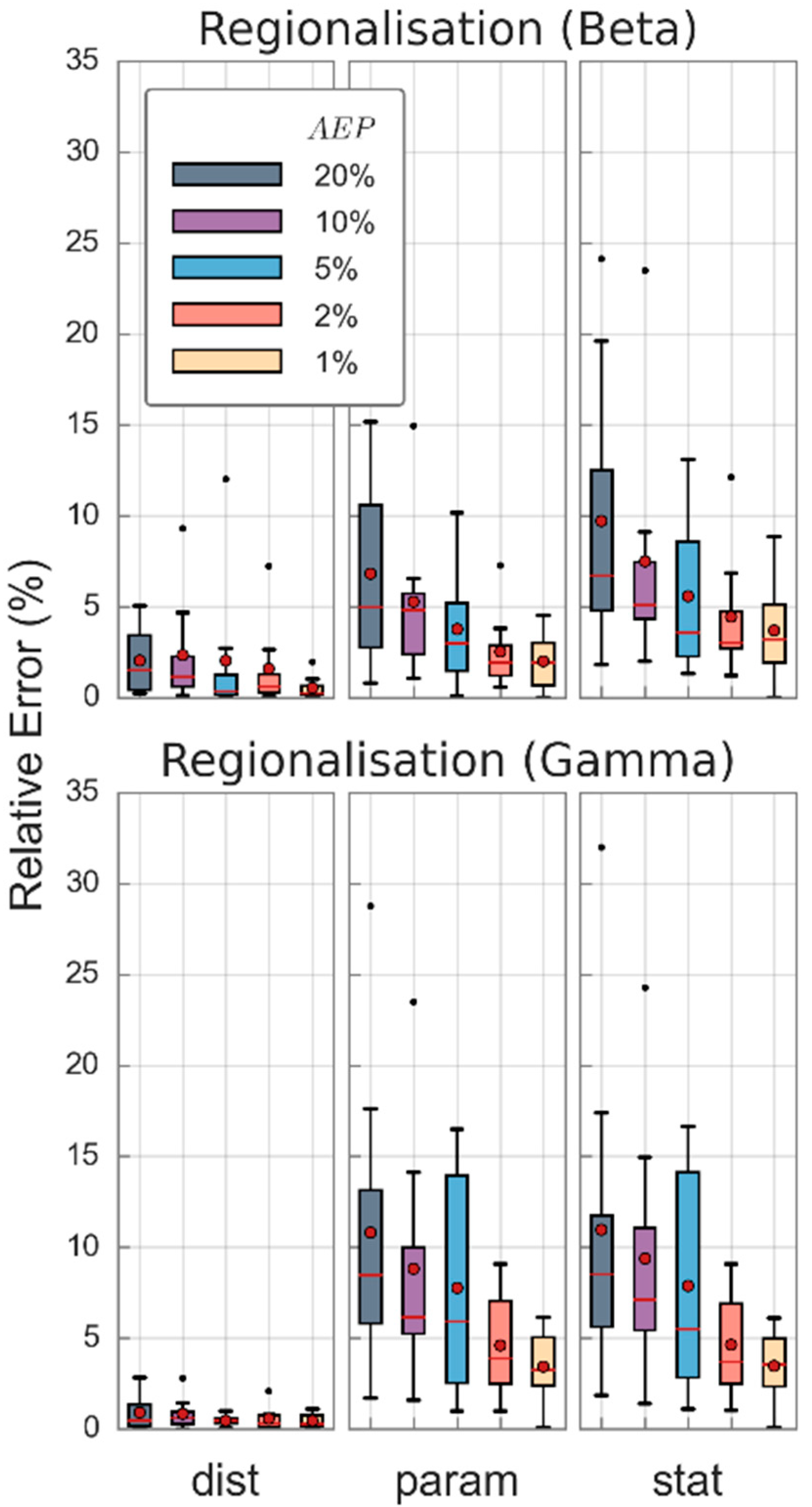
The regionalization of parametric distributions consists of three main themes; first we assume enough data are available to characterize the first two statistical moments (mean and variance), then the following two techniques assume no data are available at the site of interest, as follows:
- Regionalization of the probability distribution (dist): each candidate distribution is assumed to be the true underlying distribution at the site of interest, the first two statistical moments are derived from observed data and then the distribution parameters are estimated using the MoM.
- Regionalization of distribution parameters (param): candidate distributions are assumed to be the true underlying distribution and parameters are estimated as the average within a hydrologically similar region (where individual catchment parameters were estimated using the MLE).
- Regionalization of statistical moments (stat): the candidate distribution is assumed to be representative of the true underlying distribution, the first two statistical moments are regionalized within a hydrologically similar region and then the distribution parameters are estimated using the MoM.
Design floods are estimated using the three regionalization techniques for the eight study catchments. Resulting design floods from the three successive regionalization methods are compared using relative errors of the peak flows (Equation (7)), where the actual peak flow is taken as the design flood, estimated using a GEV distribution where parameters are estimated with the MLE and the observed annual maximum flood dataset. Results are presented in Figure 7. Regionalizing the distribution alone results in minor uncertainties. Regionalizing initial losses for catchments without data (either through the distribution parameters or data statistics) results in up to ±15% uncertainty in design flood estimates. Most of this error is most likely due to uncertainties in the mean value, with observed mean values being significantly higher than the regionalized mean values. The uncertainty in design flood estimates by our study is smaller as compared to similar previous studies. For example, the variation of mean initial loss value by 50% resulted in design flood estimates to vary in the range of 16% to 41% by Caballero and Rahman [28] for three study catchments in south-east Australia. In another study, based on eastern Australian data, a difference of up to 30% was noted between design flood estimates obtained by at-site flood frequency analysis and probability-distributed initial loss/Monte Carlo simulation approach [20,49].
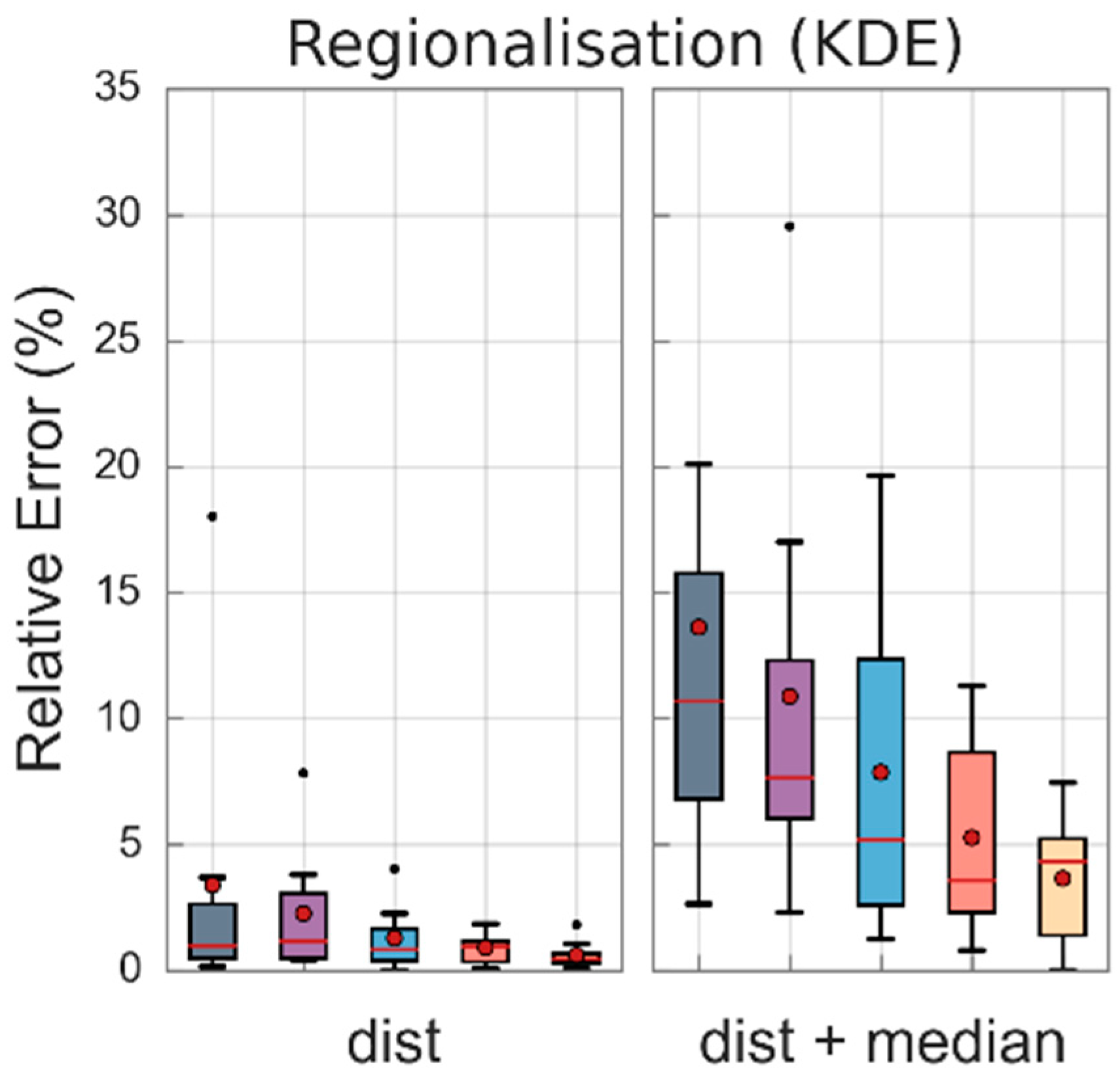
Given the freedom of nonparametric distributions to take on any functional form, the parametric regionalization methods could not be adopted. Rather, for nonparametric models two main themes were adopted; first assuming enough data are available to characterize the median value and the second assuming no data are available, as follows:
- Regionalization of the probability distribution (dist): a standardized KDE distribution is assumed to be representative of the underlying distribution and the median value is derived from the observed data; the standardized KDE distribution is derived from individual KDE distributions within a hydrologically similar region, each distribution is normalized by the median value and the average distribution is determined.
- Regionalization of the probability distribution and median value (dist + median): a standardized KDE distribution is assumed to be the true underlying distribution and the median value is estimated from within a hydrologically similar region.
Overall, relative errors in the design flood estimates using the nonparametric model appear to be higher than the equivalent for parametric models, both for catchments where sufficient data are available to characterize key statistics and where no data are available (see Figure 8).
The design flood estimates obtained in this study using regionalized initial loos values are compared with regional design flood estimates by the recommended RFFA method in the Australian Rainfall and Runoff (ARR), the national guideline. It has been found that our method provides design flood estimates that are well within the confidence limits recommended by ARR RFFE model. The absolute median relative error values considering all our eight study catchments range 17% to 22% with a standard deviation of 6% to 11%. It should be noted that due to high rainfall variability in Australia, design flood estimates at ungauged catchments are associated with a high degree of uncertainty (generally in the range of 30 to 50%) as reported in the ARR.
5.5. Conclusions
Several hypothetical probability distributions have been compared with regards to their suitability in representing the true underlying initial loss distribution. Further to this, the impact of uncertainties in probability-distributed initial losses on design flood estimates has been evaluated. Design floods were estimated using a Monte Carlo simulation technique with stratified sampling, using stochastic rainfall depths, temporal patterns, and initial losses. The main results of this study can be summarized as follows:
- The functional form of the initial loss data in Australia can be approximated using the Beta and Gamma models. These results are in line with differing outcomes in previous studies, for instance Rahman et al. [12] recommend the use of the Beta distribution to represent initial losses, while Caballero and Rahman [28] determine the Gamma distribution to be most appropriate for initial loss data.
- By setting differing thresholds for the minimum sample size of initial loss data used to derive probability distributions, mixed results were found. This highlights the importance of sample size in deriving probability distributions of initial losses.
- Design flood estimates from successive candidate distributions showed relative errors typically within ±3%, similarly by shifting the distribution mean relative errors within approximately ±20% and a change in the distribution variance also resulted in relative errors within ±3%. These results lead us to conclude that knowledge of the central tendency of distributed initial losses is more important than knowledge of the true functional form of the initial loss data.
- Larger parameter sets generally present issues in regionalization; however, the comparison of the 4-parameter Beta and 2-parameter Gamma distributions showed that this was not the case in this study. Under the assumption that the catchments were ungauged, the relative errors of the design floods using the two distributions were comparable, with the Beta model producing slightly less uncertainty.
- Regionalization of the initial loss distributions led to design floods being estimated to within ±15% accuracy, with the largest uncertainty coming from errors in regionalization of the central tendency of initial loss data. This leads us to conclude that initial loss distributions can be regionalized relatively easily; however, difficulties lie in accurate estimation of the central tendency of the distribution.
Although this study investigated the significance of the tails of the initial loss distribution (i.e., variance) on peak flow estimates, it is noted that further investigation into the impact of these tails on confidence limits where these are derived should be a topic of future research. The distribution tails would be expected to have a more substantial impact on the confidence limits rather than the peak flow estimates. Although the initial loss-continuing loss model has been adopted for runoff generation in this study, we feel that given the initial loss is simply a measure of the antecedent moisture condition these results are typical of what might be found with similar models of this type. However, more research is required to test this approach on similar models.
The current study sought to determine the feasibility of regionalizing probability-distributed initial losses and the potential effect of this regionalized initial loss data on design flood estimates. More comprehensive regionalization schemes, such as regional equations based on geographic or meteorological characteristics, are left to future research efforts.
It should be noted that due to absence of recorded streamflow data (with good quality and adequate length), no catchment was selected from interior/arid regions of Australia. Hence, the findings of this study are not applicable to these arid regions. However, most of the population and development projects in Australia are concentrated to coastal regions; the outcomes of this study, are applicable to these coastal regions, in particular eastern NSW. When good quality streamflow data are available in the arid regions, this study should be repeated with the enhanced dataset.
Only four theoretical distribution functions are adopted to regionalize initial loss data in the study area. More distributions could have been adopted; however, use of these four distributions has demonstrated that it is feasible to regionalize initial loss data in the study area. In future studies, other theoretical distribution functions should be tested.
Author Contributions
M.L. conducted the analysis, prepared the draft of the manuscript. A.R. contributed to the research idea, reviewed, and edited the write-up. All authors have read and agreed to the published version of the manuscript.
Funding
This research received no external funding.
Institutional Review Board Statement
Not applicable.
Informed Consent Statement
Not applicable.
Data Availability Statement
Data in this study can be obtained from WaterNSW and Australian Bureau of Meteorology by contacting these organisations and paying a fee.
Acknowledgments
The authors acknowledge Western Sydney University, WMA water and former Sinclair Knight Merz for their supports and input during data analysis. The authors also acknowledge Academic Editor and four anonymous reviewers whose comments have assisted to enhance the quality of the manuscript.
Conflicts of Interest
The authors declare no conflict of interest.
References
- Moore, R.J. The probability-distributed principle and runoff production at point and basin scales. Hydrol. Sci. J. 1985, 30, 273–297. [Google Scholar] [CrossRef] [Green Version]
- Hao, R.J.; Zhuang, Y.L.; Fang, L.R.; Liu, X.R.; Zhang, Q. The Xinanjiang model. In Hydrological Forecasting; Proceedings of the Oxford Symposium; IAHS: Oxford, UK, 1980. [Google Scholar]
- Bennett, T.; Peters, J. Continuous Soil Moisture Accounting in the Hydrologic Engineering Center Hydrologic Modeling System (HEC-HMS). Build. Partnersh. 2000. [Google Scholar] [CrossRef]
- Boughton, W.; Srikanthan, S.; Weinmann, E. Benchmarking a New Design Flood Estimation System. Australas. J. Water Resour. 2002, 6, 45–52. [Google Scholar] [CrossRef]
- Heneker, T.M.; Lambert, T.M.; Kuczera, G. Overcoming the joint probability problem associated with initial loss estimation in design flood estimation. Aust. J. Water Resour. 2003, 7, 101–109. [Google Scholar]
- Pathiraja, S.; Westra, S.; Sharma, A. Why continuous simulation? The role of antecedent moisture in design flood estimation. Water Resour. Res. 2012, 48, W06534. [Google Scholar] [CrossRef] [Green Version]
- Aubert, D.; Loumagne, C.; Oudin, L. Sequential assimilation of soil moisture and streamflow data in a conceptual rainfall–runoff model. J. Hydrol. 2003, 280, 145–161. [Google Scholar] [CrossRef]
- Bocchiola, D.; Rosso, R. Use of a derived distribution approach for flood prediction in poorly gauged basins: A case study in Italy. Adv. Water Resour. 2009, 32, 1284–1296. [Google Scholar] [CrossRef]
- Camici, S.; Tarpanelli, A.; Brocca, L.; Melone, F.; Moramarco, T. Design soil moisture estimation by comparing continuous and storm-based rainfall-runoff modeling. Water Resour. Res. 2011, 47, W05527. [Google Scholar] [CrossRef]
- Tramblay, Y.; Bouaicha, R.; Brocca, L.; Dorigo, W.; Bouvier, C.; Camici, S.; Servat, E. Estimation of antecedent wetness conditions for flood modelling in northern Morocco. Hydrol. Earth Syst. Sci. 2012, 16, 4375–4386. [Google Scholar] [CrossRef] [Green Version]
- Svensson, C.; Kjeldsen, T.R.; Jones, D.A. Flood frequency estimation using a joint probability approach within a Monte Carlo framework. Hydrol. Sci. J. 2013, 58, 8–27. [Google Scholar] [CrossRef] [Green Version]
- Rahman, A.; Weinmann, P.E.; Mein, R.G. The Use of Probability-Distributed Initial Losses in Design Flood Estimation. Australas. J. Water Resour. 2002, 6, 17–29. [Google Scholar] [CrossRef]
- De Michele, C.; Salvadori, G. On the derived flood frequency distribution: Analytical formulation and the influence of antecedent soil moisture condition. J. Hydrol. 2002, 262, 245–258. [Google Scholar] [CrossRef]
- Aronica, G.T.; Candela, A. Derivation of flood frequency curves in poorly gauged Mediterranean catchments using a simple stochastic hydrological rainfall-runoff model. J. Hydrol. 2007, 347, 132–142. [Google Scholar] [CrossRef]
- Kjeldsen, T.R.; Svensson, C.; Jones, D.A. A joint probability approach to flood frequency estimation using Monte Carlo simulation. In British Hydrological Society Third International Symposium: Role of Hydrology in Managing Consequences of a Changing Global Environment, Newcastle, UK, 19–23 July 2010; Kirby, C., Ed.; British Hydrological Society: London, UK, 2010. [Google Scholar]
- Saghafian, B.; Golian, S.; Ghasemi, A. Flood frequency analysis based on simulated peak discharges. Nat. Hazards 2013, 71, 403–417. [Google Scholar] [CrossRef]
- Rahman, A.; Weinmann, P.E.; Hoang, T.M.T.; Laurenson, E. MMonte Carlo simulation of flood frequency curves from rainfall. J. Hydrol. 2002, 256, 196–210. [Google Scholar] [CrossRef]
- Zheng, F.; Leonard, M.; Westra, S. Efficient joint probability analysis of flood risk. J. Hydroinform. 2015, 17, 584–597. [Google Scholar] [CrossRef]
- Li, J.; Thyer, M.; Lambert, M.; Kuczera, G.; Metcalfe, A. Incorporating seasonality into event-based joint probability methods for predicting flood frequency: A hybrid causative event approach. J. Hydrol. 2016, 533, 40–52. [Google Scholar] [CrossRef]
- Hill, P.; Thomson, R. Losses. In Australian Rainfall and Runoff; Ball, J., Babister, M., Weeks, W., Weinmann, E., Retallick, M., Testoni, I., Eds.; Commonwealth of Australia: London, UK, 2016. [Google Scholar]
- Loveridge, M.; Rahman, A. Monte Carlo simulation for design flood estimation: A review of Australian practice. Australas. J. Water Resour. 2018, 22, 52–70. [Google Scholar] [CrossRef]
- Tularam, G.A.; Ilahee, M. Initial loss estimates for tropical catchments of Australia. Environ. Impact Assess. Rev. 2007, 27, 493–504. [Google Scholar] [CrossRef]
- Rahman, A.; Haddad, K.; Kuczera, G.; Weinmann, P.E. Regional flood methods. In Australian Rainfall and Runoff; Ball, J., Babister, M., Weeks, W., Weinmann, E., Retallick, M., Testoni, I., Eds.; Commonwealth of Australia: London, UK, 2019; Chapter 3, Book 3. [Google Scholar]
- Haddad, K.; Rahman, A. Regional flood frequency analysis in eastern Australia: Bayesian GLS regression-based methods within fixed region and ROI framework—Quantile Regression vs. Parameter Regression Technique. J. Hydrol. 2012, 430–431, 142–161. [Google Scholar] [CrossRef]
- Stedinger, J.R.; Tasker, G.D. Regional hydrologic analysis, 1. Ordinary, weighted, and generalised least squares compared. Water Resour. Res. 1985, 21, 1421–1432. [Google Scholar] [CrossRef]
- Ouarda, T.B.M.J.; Girard, C.; Cavadias, G.S.; Bobée, B. Regional flood frequency estimation with canonical correlation analysis. J. Hydrol. 2001, 254, 157–173. [Google Scholar] [CrossRef]
- Gamage, S.H.P.W.; Hewa, G.A.; Beecham, S. Probability distributions for explaining hydrological losses in South Australian catchments. Hydrol. Earth Syst. Sci. 2013, 17, 4541–4553. [Google Scholar] [CrossRef]
- Caballero, W.L.; Rahman, A. Development of regionalized joint probability approach to flood estimation: A case study for Eastern New South Wales, Australia. Hydrol. Process. 2013, 28, 4001–4010. [Google Scholar] [CrossRef]
- Charalambous, J.; Rahman, A.; Carroll, D. Application of Monte Carlo Simulation Technique to Design Flood Estimation: A Case Study for North Johnstone River in Queensland, Australia. Water Resour. Manag. 2013, 27, 4099–4111. [Google Scholar] [CrossRef]
- Loveridge, M.; Rahman, A. Quantifying uncertainty in rainfall–runoff models due to design losses using Monte Carlo simulation: A case study in New South Wales, Australia. Stoch. Environ. Res. Risk Assess. 2014, 28, 2149–2159. [Google Scholar] [CrossRef]
- Ball, J.; Babister, M.; Nathan, R.; Weeks, W.; Weinmann, E.; Retallick, M.; Testoni, I. Australian Rainfall and Runoff: A Guide to Flood Estimation; Commonwealth of Australia: London, UK, 2016. [Google Scholar]
- Adamowski, K. A Monte Carlo comparison of parametric and nonparametric estimation of flood frequencies. J. Hydrol. 1989, 108, 295–308. [Google Scholar] [CrossRef]
- Scott, D.W. Multivariate Density Estimation: Theory, Practice and Visualization; John Wiley: New York, NY, USA, 1992. [Google Scholar]
- Turlach, B.A. Bandwidth Selection in Kernel Density Estimation: A Review; CORE and Institut de Statistique: Loubain, Belgium, 1993. [Google Scholar]
- Bashtannyk, D.M.; Hyndman, R.J. Bandwidth selection for kernel conditional density estimation. Comput. Stat. Data Anal. 2001, 36, 279–298. [Google Scholar] [CrossRef] [Green Version]
- Silverman, B.W. Density Estimation for Statistics and Data Analysis; Chapman and Hall: London, UK, 1986. [Google Scholar]
- Jones, M.C.; Marron, J.S.; Sheather, S.J. A Brief Survey of Bandwidth Selection for Density Estimation. J. Am. Stat. Assoc. 1996, 91, 401–407. [Google Scholar] [CrossRef]
- Lilliefors, H.W. On the Kolmogorov-Smirnov Test for the Exponential Distribution with Mean Unknown. J. Am. Stat. Assoc. 1969, 64, 387–389. [Google Scholar] [CrossRef]
- Efron, B. Bootstrap Methods: Another Look at the Jackknife. Ann. Stat. 1979, 7, 1–26. [Google Scholar] [CrossRef]
- Chernick, M.R. Bootstrap Methods—A Guide for Practitioners and Researchers, 2nd ed.; Wiley Interscience: New York, NY, USA, 2007. [Google Scholar]
- Babu, G.J.; Rao, C.R. Bootstrap methodology. In Computational Statistics, Handbook of Statistics; Rao, C.R., Ed.; North Holland Publishing Co.: Amsterdam, The Netherlands, 1993; Chapter 9; pp. 627–659. [Google Scholar]
- Hosking, J.R.M.; Wallis, J.R. Some statistics useful in regional frequency analysis. Water Resour. Res. 1993, 29, 271–281. [Google Scholar] [CrossRef]
- Laurenson, E.M.; Mein, R.G. RORB Version 3 Runoff Routing Program. Programmer Manual; Monash University: Melbourne, Australia, 1986. [Google Scholar]
- Patel, H.; Rahman, A. Probabilistic nature of storage delay parameter of the hydrologic model RORB: A case study for the Cooper’s Creek catchment in Australia. Hydrol. Res. 2015, 46, 400–410. [Google Scholar] [CrossRef]
- Jordan, P.; Nathan, R.; Seed, A. Application of spatial and space-time patterns of design rainfall to design flood estimation. In Proceedings of the 36th Hydrology and Water Resources Symposium: The Art and Science of Water, Hobart, Australia, 7–10 December 2015; Engineers Australia: Barton, ACT, Australia, 2015; pp. 88–95. [Google Scholar]
- Loveridge, M.; Babister, M.; Retallick, M. Australian Rainfall and Runoff Revision Project 3: Temporal Patterns of Rainfall; ARR Report Number P3/S3/013; Engineers Australia Engineering House: Barton, ACT, Australia, 2015; ISBN 978-085825-9614. [Google Scholar]
- Waugh, A.S. Design Losses in Flood Estimation. In Proceedings of the International Hydrology & Water Resources Symposium, Hyatt Regency, Perth, Australia, 2–4 October 1991; pp. 629–630. [Google Scholar]
- Hill, P.I.; Maheepala, U.K.; Mein, R.G.; Weinmann, P.E. Empirical Analysis of Data to Derive Losses for Design Flood Estimation in South. Eastern Australia; Monash University: Clayton, Australia, 1996. [Google Scholar]
- Hill, P.; Graszkiewicz, Z.; Taylor, M.; Nathan, R. Australian Rainfall and Runoff Revision Project 6: Loss Models for Catchment Simulation: Phase 4 Analysis of Rural Catchments; P6/S3/016B; Geoscience Australia: Canberra, Australia, 2014. [Google Scholar]
- Ilahee, M. Modelling Losses in Flood Estimation. Ph.D. Thesis, Queensland University of Technology, Brisbane, Australia, 2005. Available online: http://eprints.qut.edu.au/16019 (accessed on 27 June 2017).
- Caballero, W.L. Enhanced Joint Probability Approach for Flood Modelling. Ph.D. Thesis, University of Western Sydney, Penrith, Australia, 2013. Available online: http://researchdirect.uws.edu.au/islandora/object/uws:28537 (accessed on 27 June 2017).
Figure 1.
Location of the selected catchments in eastern New South Wales (NSW).

Figure 2.
Number of catchments in which the null hypothesis is rejected by each goodness-of-fit test, for each study dataset.
Figure 2.
Number of catchments in which the null hypothesis is rejected by each goodness-of-fit test, for each study dataset.

Figure 3.
Percentage of catchments (with sample size greater than 10) in which each candidate distribution is selected by each goodness-of-fit test, for each study dataset.
Figure 3.
Percentage of catchments (with sample size greater than 10) in which each candidate distribution is selected by each goodness-of-fit test, for each study dataset.

Figure 4.
Percentage of catchments (with sample size greater than 30) in which each candidate distribution is selected by each goodness-of-fit test, for each study dataset.
Figure 4.
Percentage of catchments (with sample size greater than 30) in which each candidate distribution is selected by each goodness-of-fit test, for each study dataset.

Figure 5.
Distribution of relative errors in design flood estimates for each quantile across the eight study catchments using five candidate distributions to represent variability in initial losses. Here KDE (kernel density estimate) represents nonparametric method and AEP stands for annual exceedance probability.

Figure 6.
Distribution of relative errors in design flood estimates for each flood quantile across the eight study catchments using distributions with the means shifted by specified percentages (Beta distribution).
Figure 6.
Distribution of relative errors in design flood estimates for each flood quantile across the eight study catchments using distributions with the means shifted by specified percentages (Beta distribution).

Figure 7.
Distribution of relative errors in design flood estimates for each flood quantile across the eight study catchments using various methods to regionalize probability-distributed initial losses (parametric models). (Here, Beta and Gamma distributions are used to regionalize initial loss distribution).

Figure 8.
Distribution of relative errors in design flood estimates for each flood quantile across the eight study catchments using various methods to regionalize probability-distributed initial losses (nonparametric model).
Figure 8.
Distribution of relative errors in design flood estimates for each flood quantile across the eight study catchments using various methods to regionalize probability-distributed initial losses (nonparametric model).


Table 1.
Geographic and meteorological catchment characteristics, including data availability for the selected study catchments.
Table 1.
Geographic and meteorological catchment characteristics, including data availability for the selected study catchments.
| Catchment | Drainage Area (km2) | Mean Annual Rainfall (mm) | Mean Annual Runoff (mm) | Catchment Relief (mAHD) | Concurrent Rainfall-Runoff Record Length (Year) | Number of Events |
|---|---|---|---|---|---|---|
| Bielsdown | 82 | 1835 | 1424 | 362 | 29 (1971–1999) | 57 |
| Leycester | 179 | 1541 | 525 | 943 | 45 (1967–2011) | 48 |
| Macquarie | 35 | 1700 | 738 | 753 | 44 (1962–2005) | 26 |
| Nowendoc | 218 | 972 | 298 | 595 | 41 (1971–2011) | 37 |
| Orara | 135 | 1890 | 946 | 801 | 40 (1970–2009) | 37 |
| Ourimbah | 83 | 1356 | 227 | 334 | 35 (1976–2010) | 38 |
| Oxley | 218 | 1531 | 721 | 1179 | 47 (1965–2011) | 53 |
| Pokolbin | 25 | 802 | 52 | 442 | 49 (1963–2011) | 36 |
Publisher’s Note: MDPI stays neutral with regard to jurisdictional claims in published maps and institutional affiliations. |
© 2021 by the authors. Licensee MDPI, Basel, Switzerland. This article is an open access article distributed under the terms and conditions of the Creative Commons Attribution (CC BY) license (https://creativecommons.org/licenses/by/4.0/).
Share and Cite
MDPI and ACS Style
Loveridge, M.; Rahman, A. Effects of Probability-Distributed Losses on Flood Estimates Using Event-Based Rainfall-Runoff Models. Water 2021, 13, 2049. https://doi.org/10.3390/w13152049
AMA Style
Loveridge M, Rahman A. Effects of Probability-Distributed Losses on Flood Estimates Using Event-Based Rainfall-Runoff Models. Water. 2021; 13(15):2049. https://doi.org/10.3390/w13152049
Chicago/Turabian StyleLoveridge, Melanie, and Ataur Rahman. 2021. "Effects of Probability-Distributed Losses on Flood Estimates Using Event-Based Rainfall-Runoff Models" Water 13, no. 15: 2049. https://doi.org/10.3390/w13152049
Note that from the first issue of 2016, this journal uses article numbers instead of page numbers. See further details here.