
Dynamic Pluvial Flash Flooding Hazard Forecast Using Weather Radar Data


1
Department of Geoinformatics, Faculty of Mining and Geology, VŠB—Technical University of Ostrava, 17. Listopadu 15/2172, 708 00 Ostrava-Poruba, Czech Republic
2
Institute of Geonics, Czech Academy of Sciences, Drobneho 28, 602 00 Brno, Czech Republic
*
Author to whom correspondence should be addressed.
Remote Sens. 2021, 13(15), 2943; https://doi.org/10.3390/rs13152943
Submission received: 2 June 2021
/
Revised: 21 July 2021
/
Accepted: 22 July 2021
/
Published: 27 July 2021
Abstract
:Pluvial flash floods are among the most dangerous weather-triggered disasters, usually affecting watersheds smaller than 100 km2, with a short time to peak discharge (from a few minutes to a few hours) after causative rainfall. Several warning systems in the world try to use this time lag to predict the location, extent, intensity, and time of flash flooding. They are based on numerical hydrological models processing data collected by on-ground monitoring networks, weather radars, and precipitation nowcasting. However, there may be areas covered by weather radar data, in which the network of ground-based precipitation stations is not sufficiently developed or does not even exist (e.g., in an area covered by portable weather radar). We developed a method usable for designing an early warning system based on a different philosophy for such a situation. This method uses weather radar data as a 2D signal carrying information on the current precipitation distribution over the monitored area, and data on the watershed and drainage network in the area. The method transforms (concentrates) the 2D signal on precipitation distribution into a 1D signal carrying information on potential runoff distribution along the drainage network. For sections of watercourses where a significant increase in potential runoff can be expected (i.e., a significant increase of the 1D signal strength is detected), a warning against imminent flash floods can be possibly issued. The whole curve of the potential runoff development is not essential for issuing the alarm, but only the significant leading edge of the 1D signal is important. The advantage of this procedure is that results are obtained quickly and independent of any on-ground monitoring system; the disadvantage is that it does not provide the exact time of the onset of a flash flooding or its extent and intensity. The generated alert only warns that there is a higher flash flooding hazard in a specific section of the watercourse in the coming hours. The forecast is presented as a dynamic map of the flash flooding hazard distribution along the segments of watercourses. Relaying this hazard to segments of watercourses permits a substantial reduction in false alarms issued to not-endangered municipalities, which lie in safe areas far away from the watercourses. The method was tested at the local level (pluvial flash floods in two small regions of the Czech Republic) and the national level for rainfall episodes covering large areas in the Czech Republic. The conclusion was that the method is applicable at both levels. The results were compared mainly with data related to the Fire and Rescue Service interventions during floods. Finally, the increase in the reliability of hazard prediction using the information on soil saturation is demonstrated. The method is applicable in any region covered by a weather radar (e.g., a portable one), even if there are undeveloped networks of rain and hydrometric gauge stations. Further improvement could be achieved by processing more extended time series and using computational intelligence methods for classifying the degree of flash flooding hazard on individual sections of the watercourse network.

1. Introduction
In general, flash floods usually occur in very small, typically ungauged, watersheds (with a few tens of square kilometres). They are characterised by rapid onset (with water levels in the drainage network reaching a crest within a few minutes to a few hours after the beginning of the causative rainfall [1,2,3,4]). This time is usually too short to activate the emergency response units and effectively prevent damage to human activities, properties, and life [5,6,7]. Jonkman, in his study [8], as well as World Meteorological Organisation in [9], showed that the mortality from flash floods (the number of fatalities divided by the number of affected persons) is higher than that of other natural hazards. That is why forecasting the hazard of flash flooding is an essential component of public safety and quality of life [10].
The flash flooding forecast system can perform predictions quantitatively or qualitatively. Qualitative prediction strives to predict the expected occurrence of the flash flood event in an area of interest in the near future, with no or very few details about the real situation development [11]. In contrast, quantitative prediction is focused on the forecast of the time of flood occurrence and the expected extent of the flooded area.
Quantitative prediction systems are usually based on physical process models [9]. These models use a mathematical description of physical processes taking place within some phases of the hydrological cycle. They can be either lumped (a sub-basin that is characterised by one value of each geomorphological or hydrological parameter) or distributed (a spatial distribution function that is defined for each geomorphological or hydrological parameter, usually in the form of a raster; each raster cell is assigned a specific value of the represented parameter). The necessary condition for their use is the availability of sufficiently detailed geomorphological and hydrological data, the need to extrapolate the model to ungagged locations, and the entry of rainfall as spatially distributed, e.g., in the form of meteorological radar data. These conditions are met mainly in populated areas.
The alternative option, which has been developed especially recently, is a warning system based on data-driven models [9]. These models are based on the analysis of a large volume of data describing the studied system. The primary purpose of these models is to find the relationships between the input and output variables of the system without explicit knowledge of its behaviour [12]. Machine learning methods such as artificial neural networks, support vector machines, genetic algorithms, and others are very often used for this purpose. The result can be, for example, river flow prediction based on knowledge of weather parameters and actual hydrological conditions [13].
The data-driven models are generally simpler, easier to calibrate, and based on a long time series of measured parameters, but on the other hand, they are untrustworthy for many end-users. Firstly, because they are not based on a mathematical description of the physical processes taking place in the river basin, and secondly because it is uncertain to what extent they are reliable outside the time interval of the historical data used for their training. Another disadvantage is the non-transferability of trained models to other geographical areas with different conditions [14]. They are usable if the predicted quantities are in the gauged river section, the time series of historical data are long enough, and predictions are required only for the near future. A brief overview of different kinds of models used for flood forecasting is in [15].
No matter what kind of model is in the background, the forecasts must be fully automated in the case of flash floods due to the need for the shortest possible forecast update interval (5–10 min). Manual control or modification of the input data and any adjustments to the model’s parameters in real-time are impossible [16]. From an operational perspective, priority should be given to the capability of predicting the rising hazard of the flash flooding occurrence, unlike for riverine floods, where the priority is the prediction of their time, magnitude and flooded area extent [17]. This hazard prediction should be targeted to support informed decision-making [18,19].
Many systems for flash flooding forecasting are active in the world [1,7,20,21,22,23]. The widely used Automated Local Evaluation in Real-Time (ALERT) was developed in the USA [24]. The National Weather Service developed ALERT in the 1970s as a local system of flood warnings for smaller areas, such as a county or city. These systems have relatively low operating costs and provide real-time information about precipitation and flow rates that enable flood hazard assessment. Individual cities or counties own and operate these systems, and the National Weather Service provides technical support. One of the main components of these systems is the rain gauge, which offers real-time precipitation information. These systems can also be equipped with water level sensors, temperature sensors, and wind sensors. They are used in most of the western states of the US, especially in California and Arizona [24]. Similar systems were developed for and are operated by many mountainous municipalities worldwide.
Another methodology for the periodical evaluation of flash flooding hazard is called the Flash Flood Guidance system (FFG) [25,26]. FFG was one of the first methods developed for the prediction of flash floods [27]. The Hydrologic Research Centre in the USA designed and developed the FFG. This system is based on weather radar sensed precipitation, initial soil moisture conditions, and a hydrological model running in the inverse mode. It tries to determine the amount of precipitation of a given duration necessary to produce an overflow of the riverbank [7]. A typical product is called the Flash Flood Guidance (FFG), represented as a grid 1 × 1 km, describing the rainfall of a given duration over a small watercourse basin, which is needed to create flooding. Alfieri et al. [28] described a system based on the COSMO-model, a non-hydrostatic atmospheric prediction model used in limited areas and based on simple thermal-hydrodynamic equations describing the air compressibility in a humid atmosphere. Different physical processes are taken into account in the model parameterisation [29]. The procedure for forecasting flash floods consists of many steps, from a qualitative 5-day regional prediction to local quantitative information with a lead time of a few hours. Other approaches based on weather radar data and models are described in [30,31].
An operational early warning system for flash floods runs at the European scale—the European Flood Awareness System (EFAS) [32]. EFAS includes a weather radar-based module for flash flood early warning developed in the project ERICHA ([33] in [7], www.efas.eu (accessed on 26 July 2021)). This module derives flash flooding hazard from the upstream basin-aggregated rainfall by comparing the threshold provided by climatology. More information on flood forecasting techniques and systems can be found in [15].
In the last few years, special early warning systems are under development, focused on urbanised areas. These systems work with spatial resolution up to one square kilometre both in precipitation data and models. Thus, they are beyond our considerations. A brief overview can be found, e.g., in [34,35,36].
There are two potential disadvantages of the implemented flash flooding forecast systems in this framework. (1) They rely on the well-developed on-ground precipitation monitoring network and hydrological models. However, this may not be the case in less developed areas [37]. (2) They relate flash flooding warnings to areas delineated either naturally (such as watersheds) or administratively (such as counties). This feature is quite problematic (see [38]). If the warning is issued, for example, for the whole county, it also applies to municipalities that are very far from any watercourse and are, thus, at worst endangered by overland runoff, which usually does not threaten people’s lives. The warning is essential only for municipalities near watercourses because there may be a sharp increase in the level of runoff and risk to property, but especially to human lives. Therefore, finding a way to link warnings to endangered watercourses would be appropriate.
Before developing a flash flooding forecasting system, realistic aims should be established. These aims should balance scientific and practical feasibility with end-user requirements ([39] in [35]). The present study aims to provide a straightforward method for forecasting the flash flooding hazard using raw weather radar data and watercourse network only and relating it to watercourse segments. The method allows relatively quick identification of sections of watercourses that may be endangered by flash flooding within minutes to hours. The hazard is visualised as a dynamic map of the flash flooding hazard distribution on the watercourse segments for the near future. Based on this map, a responsible person can evaluate if identified hazard endangers some human lives or property, i.e., if they are at risk. Then, potentially endangered municipalities can be warned. Practical tests demonstrate the applicability of the developed method on the local and national levels.
2. Materials and Methods
The intensity of flooding is directly linked to heavy rainfall and the antecedent moisture condition in the river basin. Mainly, the abundant rainfall during the previous time (days to weeks) determines soil saturation. High soil saturation forces rainfall to create overland runoff (e.g., [40,41]). Therefore, continuous precipitation monitoring is essential when dealing with flash floods.
2.1. Monitoring Precipitation
Significant progress has been made in monitoring the current meteorological situation [42,43,44]. A network of rain gauge stations has long measured the intensity of the precipitation. It is a direct measurement method, providing a long time series at specific locations equipped with a precision measurement instrument. Currently, measurements and data collection are often fully automated, and the measured data are usually available every 15 min [44].
In the context of heavy rainfall monitoring, the principal disadvantage of the rain gauge network is its sparseness. The distance between rain gauge stations varies from kilometres to tens of kilometres. For example, there are about 255 automatic rain gauge stations in the Czech Republic, so each station represents an area of about 300 km2 on average. The average distance between rain gauges is about 20 km. The size of intense rainfall storm cells is often in the order of kilometres [45]. That is why the system of rain gauges is not suitable for monitoring rainstorms; they can easily fall outside of rain gauge stations [2,4,46,47,48,49,50]. If we still decide to use this network to monitor torrential rains, the recommended density is one rain gauge station per square kilometre, especially for urbanised areas ([51] in [52]).
However, there is an indirect method for mapping the precipitation field based on remote sensing principles. Specifically, these are weather radars that provide an indirect estimate of the distribution of precipitation [43,44,53,54].
Using a weather radar for precipitation monitoring is quite helpful because the radar provides information about the spatial and temporal distribution of the precipitation [55] and can monitor even storm cells. These radar measurements give an instant overview of the precipitation field’s structure, development, and movement with a temporal resolution of up to 5 min and spatial resolution of 0.25 to 1 km [7,10,45]. As a result, the weather radar allows instant mapping of hazardous phenomena associated with convective clouds, such as hail and thunderstorms. On the other hand, in a convective situation, which is a common cause of heavy rainfall, the error of measuring rainfall by radar can be as much as tens of per cents (which also applies to rain gauges). The error of nowcasting based on such data can, of course, be even higher [16].
Calculation of radar precipitation estimates for a given period is performed using the radar reflectivity Z with the Marshall–Palmer relationship:
where I is the intensity of precipitation and a and b are the experimentally determined coefficients, whose values are usually set to a = 200 and b = 1.6 [43,54]. The Czech Hydro-Meteorological Institute uses these values for radar rainfall estimates as well [56]. Coefficients a and b are independent of a rain rate. They may vary from location to location and from season to season. In some sense, they reflect the climatological character of a particular location or season. However, it is challenging to determine locally specific values of these coefficients without special equipment [57]. For a reliable calculation of the precipitation intensity, the reflectivity shall be measured as close to the earth’s surface as possible. Typically, data from 1.0 to 1.5 km above the earth’s surface or the maximum reflectance in a vertical column are used. The measurement allows us to estimate the distribution of precipitation intensity. Estimated values are interpolated into a square grid, e.g., 1 × 1 km. The total rainfall over a long time (e.g., hours) can be determined by summing up a series of measurements, but this operation, unfortunately, can accumulate especially systematic errors.
Z = a × Ib
The estimation of ground precipitation intensity based on radar reflectivity Z measurements is burdened with many uncertainties, increasing with increased distance from the weather radar. The resulting precipitation estimates may, therefore, be significantly overestimated or underestimated [16,35,58]. The analysis, quantification, and impact of these uncertainties on the accuracy of the derived precipitation values have been discussed in numerous publications (e.g., [54,58,59,60,61]), but research in this area is still running [35].
One of the most frequently used techniques to eliminate errors from radar measurements is the adjustment of precipitation intensity estimates using data obtained from rain gauge stations [62,63,64,65,66,67,68,69]. Given that our proposed method is suitable mainly to areas with no or minimal network of rain gauge stations, we do not use the procedures mentioned above for improving the quality of weather radar data.
2.2. Data Sources
We used the following datasets for the implementation and reliability testing of this methodology (see Table 1):
- Hydrological division, including low-level river basins;
- Stream network;
- Weather radar data;
- Saturation indicator
- Data from hydrometric stations;
- The database of the Fire Rescue Service of the Czech Republic.
The hydrological division describes the subdivision of the Czech Republic’s territory into individual low-level river basins, and the stream network represents the backbone streams of these low-level river basins. The Water Research Institute of Tomas Garrigue Masaryk manages and distributes both datasets [70]. The scale of this data is 1:10,000.
The weather radar data described four rainfall episodes (Table 2), and the saturation indicator was accessible on 6 August 2010, 08:00 CEST, 10 June 2013, 08:00 CEST, and 26 May 2014, 08:00 CEST. The Czech Hydro-Meteorological Institute provided all of these datasets. The spatial resolution of weather radar data is 1 × 1 km. These data were collected by two weather radars covering the whole territory of the Czech Republic seamlessly (with the lowest usable beam 1500 m above the ground) [56].
For the reliability testing of the results of the developed methodology, data from two sources were used:
2.3. Proposed Methodology of Flash Flooding Hazard Prediction
The existing approaches to forecasting flash floods rely on ground monitoring systems and hydrological models to predict and quantify heavy rainfall and then quantitatively model the response of a watershed to the expected heavy rainfall. The resulting warnings are usually related to naturally delineated or administrative areas, so they are often issued for not endangered municipalities.
The presented research is based on a different philosophy. It aimed to find a method that operates on minimum input data, does not rely on rainfall-runoff models or nowcasting, will only predict the hazard of the possible flash flooding occurrence, classifies the level of hazard solely qualitatively, and relates the rising hazard to watercourse segments to limit the number of the warned municipalities. The resulting process should be robust enough and not sensitive to specific local conditions. Such a procedure should apply especially to areas for which there is no on-ground precipitation monitoring network or detailed information about the morphological and hydrological properties of the landscape and, therefore, for which it would be impossible to create a fully-fledged rainfall-runoff model. This feature would be the indisputable advantage of the developed method.
Sherman formulated the theory of unit hydrograph (UH) in the 1930s ([71,72] in [73]). UH is governed by the principle of invariance and superposition. The first one means that the response of the river basin to the same distribution of precipitation is constant; the second one means that the runoff at a given location can be built up by the superposition of runoff generated by rainfall for particular periods. Pilgrim ([74] (p. 493) and [75]) published another essential finding that at higher flows, the travel times and average velocities are almost constant. Thus, a river basin behaves linearly so that its overall response to precipitation can be derived as the sum of the reactions of the individual sub-basins. In addition, for larger river basins (more than 10 km2), where the importance of channel routing effects is growing, we can consider that overland flow can reach the backbone watercourse in a single time step [76].
The proposed method is based on similar principles on which the UH theory is based. In contrast, however, the method does not quantify both the peak flood discharge and the real-time course of the outflow. No hydrogram is created.
When we designed the proposed method, we used the following assumptions and simplifications:
- Division of the monitored area into subareas—sub-watersheds, which are perceived as homogeneous spatial units;
- For each sub-watershed, a backbone watercourse is defined, discharging water entering the sub-watershed either in the form of precipitation or inflow from the upstream sub-watershed;
- The backbone watercourse of each sub-watershed represents the smallest spatial unit used to evaluate the flash flooding hazard—the watercourse segment;
- For each sub-watershed or segment of a watercourse, a simple routing response function is defined, allowing for the response of any segment of a watercourse to heavy rainfall to be derived in the form of a measure of the flash flooding hazard,
- Assumption of linear outflow behaviour;
- Assumption of a constant and same outflow velocity;
- Mutual independence of contributions from individual sub-watersheds;
- The direct proportion of the degree of flash flooding hazard to the volume of precipitation flowing through a segment of a watercourse;
- Replacement of precipitation measurements over the monitored area with raw weather radar data.
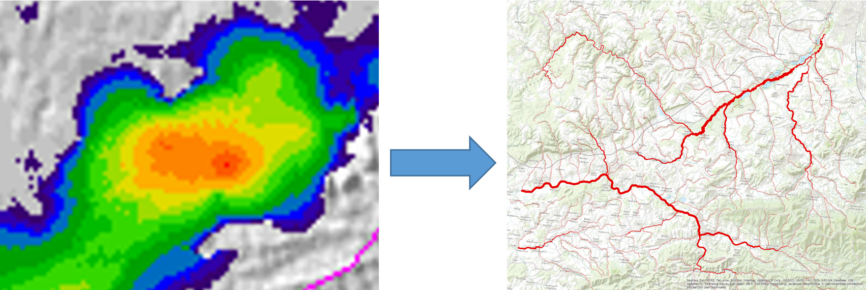
Thus, the method works with raw data of the weather radar, which is viewed as a 2D signal carrying information on the current spatial distribution of precipitation over the monitored area, and data on the watershed and drainage network in the area. The 2D signal on the precipitation distribution is transformed (concentrated) into a 1D signal carrying information on the potential runoff distribution along the drainage network.
For this transformation, routing was defined in the network of watercourse segments in the monitored area, represented by a weighted tree-type graph. The routing transforms the 2D signal registered above the sub-watershed area during the basic evaluation time step (as the sum of the raw radar reflections for all records falling into this time step) into a 1D signal representing the runoff through the backbone watercourse. This 1D signal is immediately propagated through a network of watercourse segments downstream to a distance corresponding to the outflow velocity in the channel and the selected outflow summation interval. It is assumed that the outflow in the riverbed is moving with the constant and same velocity. The 1D signal from the individual tributaries gradually accumulates. Finally, each segment is weighted by the cumulative value of the 1D signal per outflow summation interval.
The whole curve of the cumulative 1D signal development over a watercourse segment is not essential for issuing the alarm; only the occurrence of a significant leading edge of the cumulative 1D signal matters. If the signal strength exceeds the lower flash flooding limit, the degree of flash flood hazard for the given segment is set to the level of increased hazard. If the signal strength exceeds the upper flash flood hazard limit, then the hazard level is set to a high hazard value. The overall forecast is presented as a dynamic map of flash flooding hazard distribution along the watercourse segments.
The advantage of this approach is that the flash flooding hazard can be evaluated even in areas where it is not currently raining. The disadvantage is that the procedure does not provide the exact time of the onset of a flash flooding or its extent and intensity. The generated alert only warns that there is a higher flash flooding hazard in a specific section of the watercourse in the coming hours.
We assumed that all stormwater flows into the watershed backbone watercourses in this approach, so we omit infiltration. In principle, this is the worst-case scenario, describing the worst possible development of the situation. This approach corresponds to the third variant of the Beven and Kirby concept of contributing area [76].
It can be expected that the worst-case scenario will overestimate the flash flooding hazard. This overestimation can be reduced by adding information about the antecedent moisture condition in the river basin. The Czech Hydro-Meteorological Institute publishes the indicator representing soil saturation regularly every day from April to October [77] as a grid describing the distribution of saturation indicator values over the territory of the Czech Republic. The saturation indicator is expressed qualitatively using the following six-level scale: very low saturation, low saturation, saturation to water retention capacity, high saturation, very high saturation, and extremely high saturation. The methodology used to create the map of the saturation indicator is based on a simple balance model of rainfall, runoff, and evapotranspiration. The Czech Hydro-Meteorological Institute began to conduct regular assessments of this parameter in 2010 [77].
3. Data Processing
The proposed method uses the following parameters, the values of which need to be set. These are:
- The basic time step of evaluation for the summation of precipitation tb;
- The outflow velocity in the channel vw;
- The time interval for the outflow summation ts;
- The lower and upper flash flooding hazard limits.
The basic time step of evaluation for the summation of precipitation tb was set to 30 min. The basic time step of radar data collection is 5 min. The summation of the six time slices can help to reduce at least the impact of random errors in radar data.
The outflow velocity in the channel vw was set to 10 km/h. This value is based on practical evaluation of flash flood events and simulations of ungauged watersheds [78,79] and using data from hydrometric gauge stations situated on watercourses flowing through areas affected by flash floods. Different mean velocities are mentioned by Costa [80] (p. 335): 12.5 to 36.0 km/h, based on a broad study of the hydraulic characteristics of the most significant flash floods measured on small basins (less than 400 km2) by the US Geological Survey. However, these floods all occurred in semiarid to arid areas, whereas the Central European region is humid, so we used lower velocity in the channel.
The time interval for the outflow summation ts along segments of watercourses is when we assume stormwater will arrive at the given section of the watercourse. This time is expressed as the number of the basic time steps:
nt = ts/tb
The value of this parameter was set based on the expected size of the watersheds hit by flash floods. In the Czech Republic, these watersheds typically have hundreds of square kilometres, and the length of the watercourses flowing through them is tens of kilometres. The sensitivity of the proposed procedure to the values of the parameters vw and nt was verified by testing as described later (see Section 4.1).
The lower and upper flash flooding hazard limits were set for our testing based on knowledge of the impacts of flash floods on the affected areas at the test sites. For a real application, it will be necessary to develop some procedures for their setting. This issue will be discussed in more detail in Section 5.
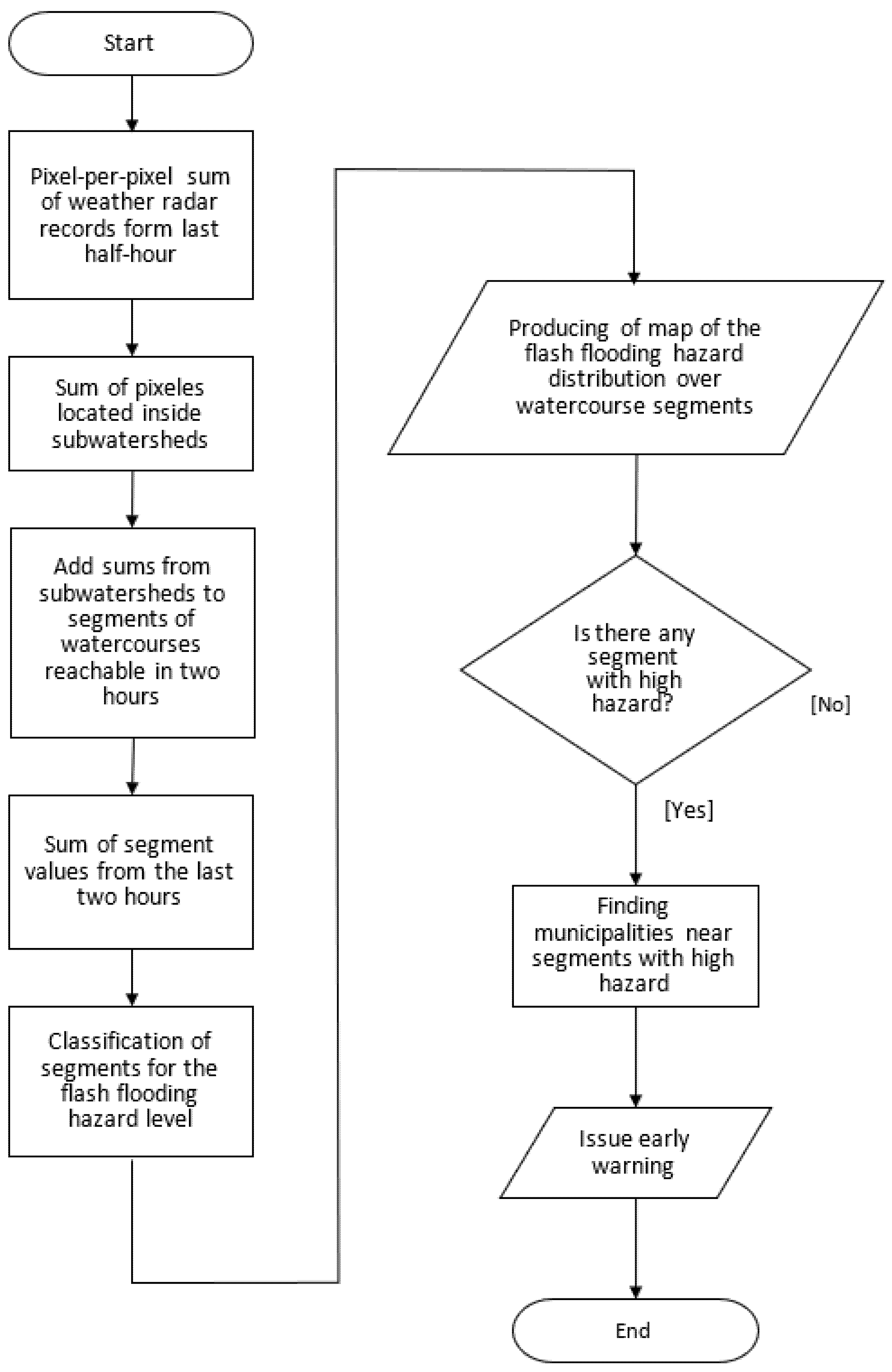
The proposed procedure calculates every half hour (tb) the pixel-by-pixel sum of weather radar records gathered in this half-hour. In the next step, the sum of the pixels located inside each sub-watershed is calculated. The result estimates the precipitation that has fallen on each sub-watershed and flows into the backbone watercourse of the sub-watershed. These values are propagated to downstream segments. The maximum distance of this propagation is given as a product of the estimated average water flow velocity in the watercourse vw and the estimated outflow summation time in watercourses ts.
In the last step, we sum up the last four processed half-hour intervals for each section of the watercourse. We get an estimate of the intensity of channel runoff represented by the strength of the 1D signal (expressed as a dimensionless number), which is interpreted as the flash flooding hazard for every segment. Sections of the watercourses are classified into the following three categories: minimal hazard (blue/narrow grey), increased hazard (black), and high hazard (red/wide grey). We use the same thresholds for the whole evaluated region, based on the findings of Benson [81] (p. D65) that with higher recurrence intervals of a flood (therefore the also higher magnitude of runoff), the relation of flood peaks variability to basin characteristics decreases. The result is a map of the distribution of the flash flooding hazard along sections of watercourses (see, e.g., Figure 2). The flowchart of the whole procedure is shown in Figure 3.
Alternatively, we can visualise the leading edge of the flash flooding hazard development for every section of the watercourse (Figures 4–9 and Figure A2, Figure A3 and Figure A4).
If the hazard is high on a particular watercourse segment, a warning can be issued to municipalities near these watercourse segments.
4. Results
4.1. Case Studies: Reliability Testing on a Local Scale
We chose two rainfall episodes that resulted in catastrophic flash floods for detailed verification of our procedure. The first episode hit Novojičínsko area on 24 June 2009 [82], particularly the town of Jeseník nad Odrou, and the second one severely impacted municipalities in the Frýdlant spur area on 7 August 2010 [83].
4.1.1. The Novojičínsko Area
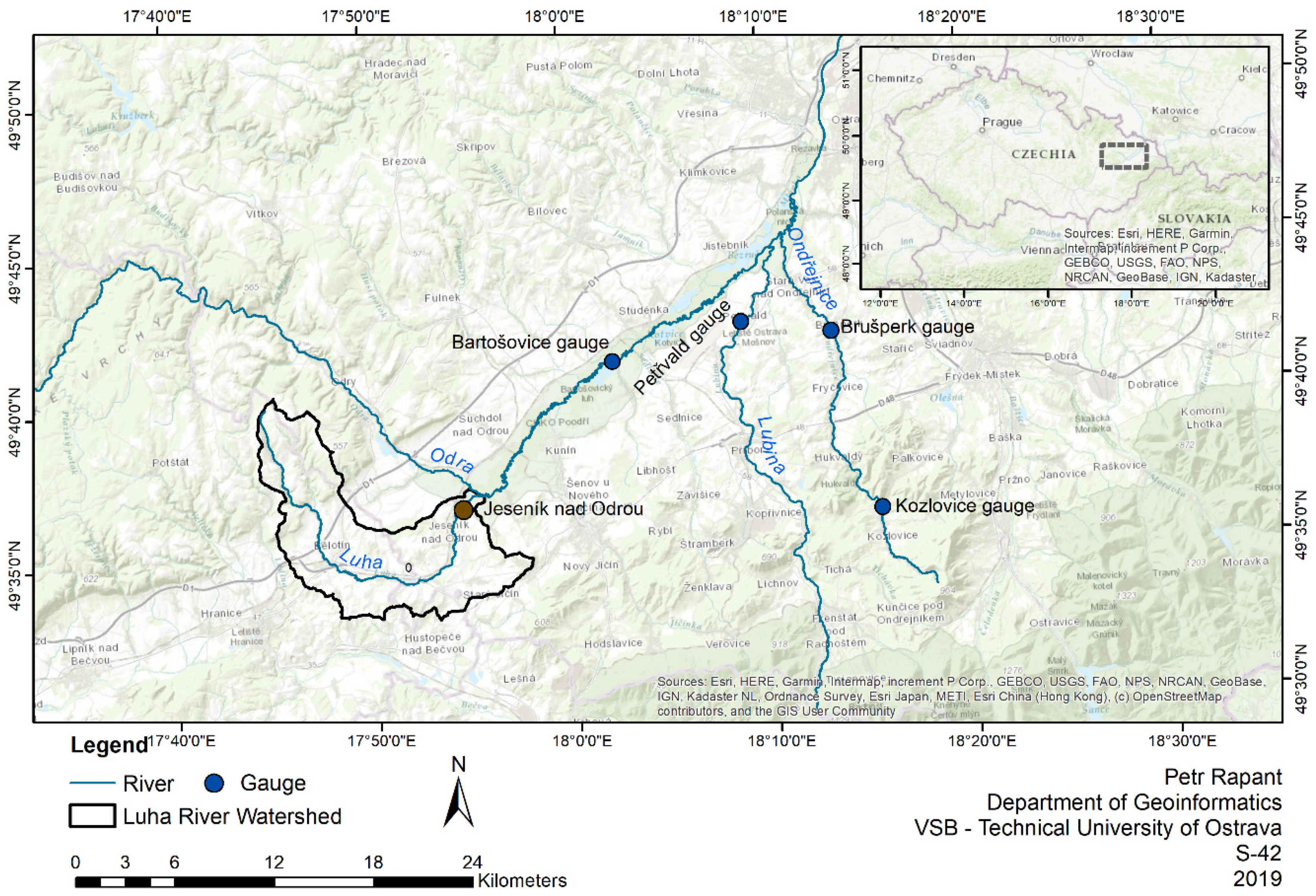
The Novojičínsko area was hit by a heavy storm on 24 June 2009. The most affected part was the Luha River Basin (Figure 1) in the Odra River Basin, approximately 60 km southwest of the city of Ostrava in the north-eastern part of the Czech Republic. The municipality of Jeseník nad Odrou lies in the lower reaches of the Luha river. There was a loss of human lives and extensive property damage in the municipality caused by the investigated heavy rainfall episode.
The cause of the extreme rainfall activity was a convective cell, part of an extensive cloud belt spread from the southwest to the northeast. The cloud belt had an approximate length of 300 km and roughly tracked the mountain range on the western edge of the Western Carpathians. A cell adjacent to the Luha River Basin arose shortly before 16:00 CEST, according to radar records from the CHMI. More intense rainfall occurred after 18:00 CEST. The centre of the very intense rainfall moved very slowly across the Luha River Basin from NE to SW between 19:00 and 21:00 CEST. Subsequently, between 23:00 CEST and 01:00 CEST the following day, the rainfall ceased. The course of flash flooding was affected by regional rainfall in the previous week, which completely saturated the soil. Therefore, no infiltration occurred during the studied rainfall episode, and all rainfall flowed directly into the watercourses (thus, the worst-case scenario in the case).
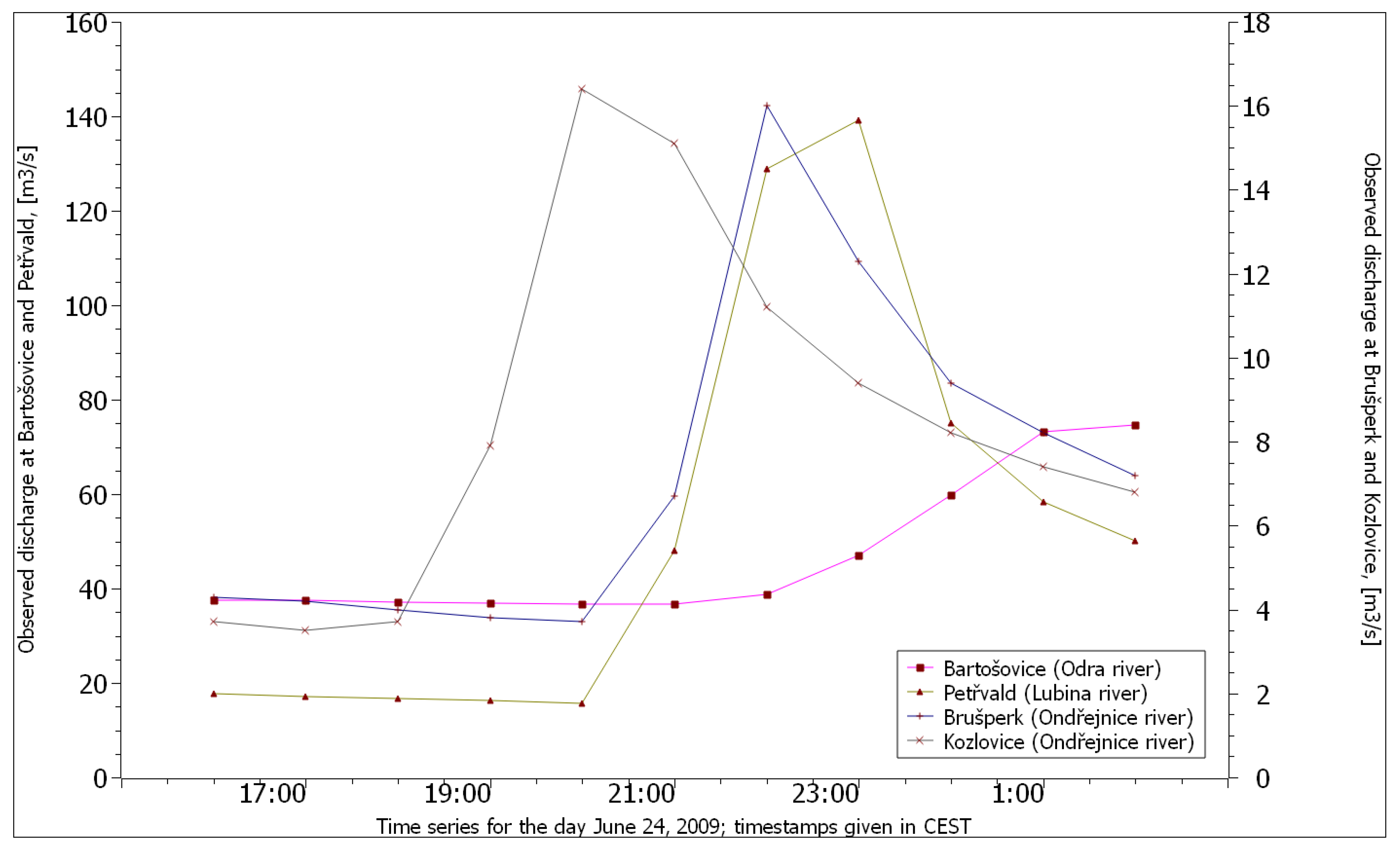
The situation on watercourses during a flash flood was described by data from hydrometric stations provided by the Odra River Basin Management Company. The hydrometric stations are located at Bartošovice on the Odra River, Kozlovice and Brušperk on the Ondřejnice River, and Petřvald on the Lubina River (Table 2, Figure 1 and Figure 4).
Figure 4 shows that the river Odra, a major watercourse in this area, seamlessly absorbed the storm outflow from individual tributaries. On the contrary, in the profile Kozlovice on the river Ondřejnice, there was a sharp increase in the flow rate after 18:00 CEST, culminating at 20:00 CEST. This culmination occurred approximately two hours later in Brušperk. Similarly, in the profile from Petřvald on the river Lubina, there was a sharp increase in the flow at 21:00 CEST. In all of these cases, water levels increased sharply, reached a short peak, and rapidly declined. This development is typical for flash floods caused by heavy rainfall.
Figure 5 shows the leading edges of the predicted flash flooding hazard in the individual section of the watercourses in the affected area, passing through the abovementioned hydrometric station. We can observe a very similar trend between the forecasted flash flooding hazard and the actual measured river flows (Figure 4). The only exception is the Bartošovice gauge station. We can see the different pattern between the rising limb of the predicted hazard and actual flow. The catchment area of this gauge station is 913 km2. The catchment area of the sub-watersheds that was hit by heavy rain, belonging to the Bartošovice station, is 214 km2. The influence of the affected area on the total flow through the Bartošovice station is, therefore, limited.
Comparing the Forecasted Hazard and Actual Flow Development
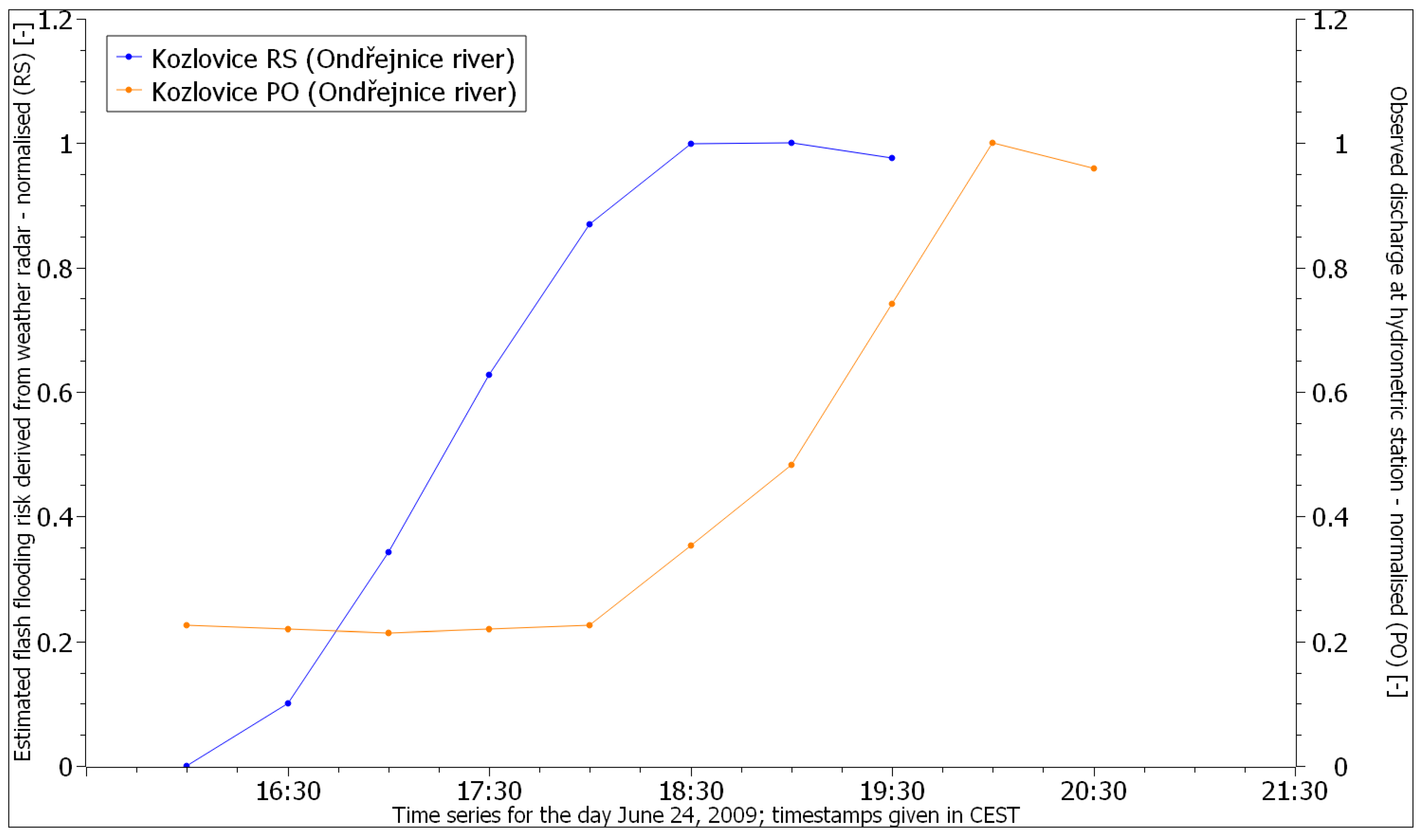
The first comparison was made at the hydrometric station in Kozlovice. We used the leading edge of the forecasted flash flooding hazard (marked as RS, data from the weather radar) and graphically compared it with the leading edge of the real flow curve (marked as PO, data from the hydrometric station; Figure 6). To ensure comparability of both curves, we converted them into a normalised scale with values between 0 and 1, determined by dividing the values of each curve by the maximum value of the respective curve.
Figure 6 shows that the leading edges of the two curves are quite similar in shape, but they are shifted in time. We consider this time shift important. It allows us to evaluate the development of the flash flooding hazard and, if necessary, issue an early warning to potentially vulnerable communities near hazardous segments of the watercourses. The lead time between the prediction and reality, if we visually compare the peaks of both curves, is approximately 2 h in the case of Kozlovice (Figure 6). We used cross-correlation to evaluate this time shift objectively. It is commonly used for these purposes in digital signal processing (we treat both curves as signals carrying information either on flash flooding hazard or on natural outflow). Cross-correlation is a measure of the similarity of two signals as a function of the shift of one relative to the other. The flash flooding hazard is shifted in time step-by-step forward to the normalised observed discharge. The cross-correlation shows that the best fit is attained with a time shift of two hours (see Table 3). A correlation coefficient value equal to 0.99 means a perfect match of both curves.
We processed data from other hydrometric stations and obtained similar results. The time lag between the real and predicted leading edges differed slightly depending on the distance of the hydrometric gauge station from the area hit by the rainfall.
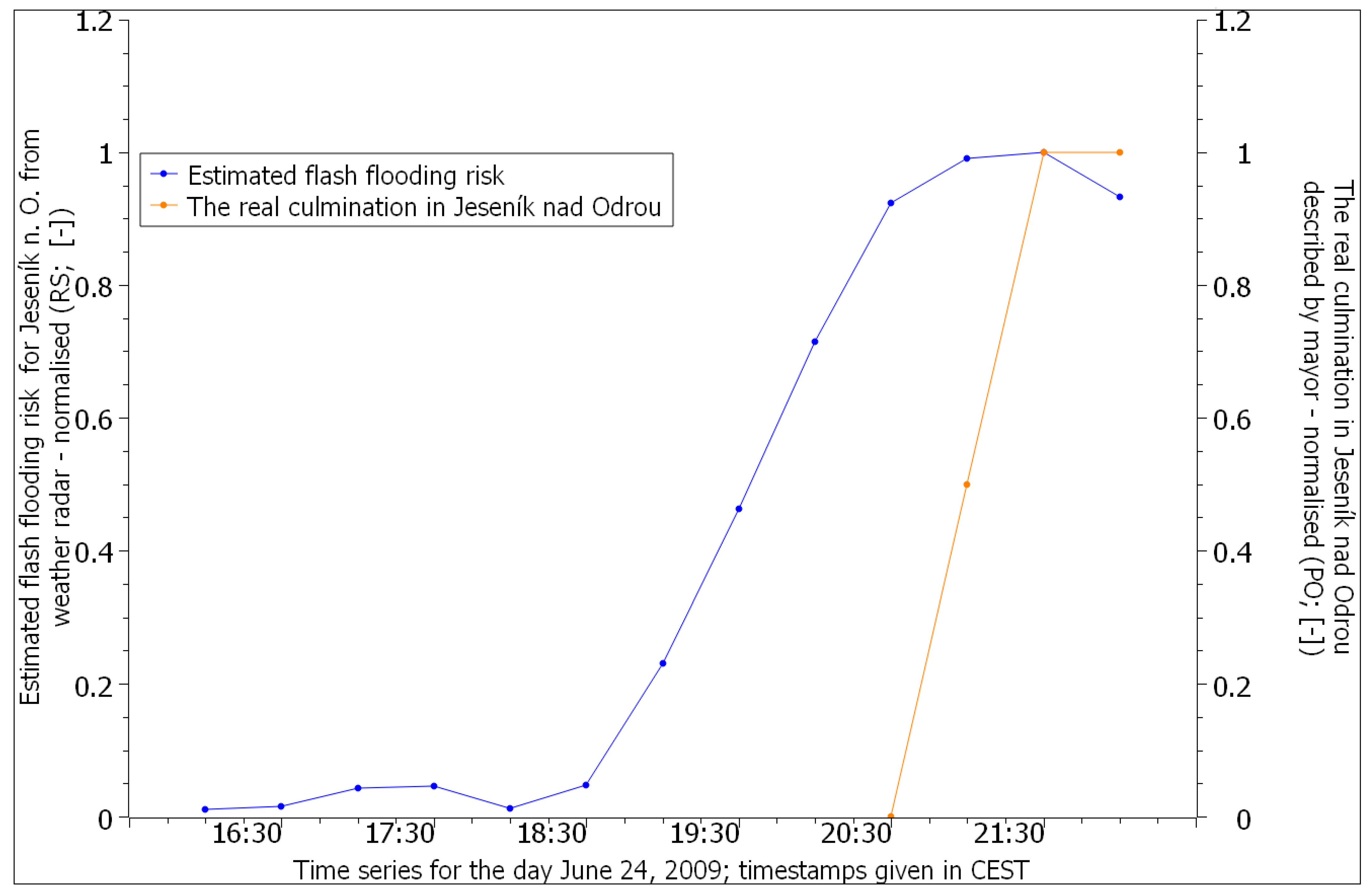
Validation of the Proposed Procedure in the Luha River Watershed
The Luha River Basin is ungauged, but we obtained a detailed description of the evolution of the flood from the mayor of the Jeseník nad Odrou municipality. Figure 7 compares the leading edge of the predicted normalised flash flooding hazard with the real leading edge as described by the mayor. The figure shows that the two curves are minimally shifted in time. However, by 20:00 CEST at the latest, it would have been possible to predict that there would be a sharp increase in the level of the Luha river within hours. Thus, it would have been possible to issue an early warning to the municipality’s mayor that a torrential flood wave was highly likely to arrive in Jeseník nad Odrou very soon. The exact arrival time of the flood wave is not possible to predict using the proposed procedure. However, the lead time of the warning would be sufficient to ensure that the mayor had enough time to inform citizens, organise evacuations to safer areas and avoid casualties. The cross-correlation (see Table 4) shows that, in reality, the lead time was one and a half hours.
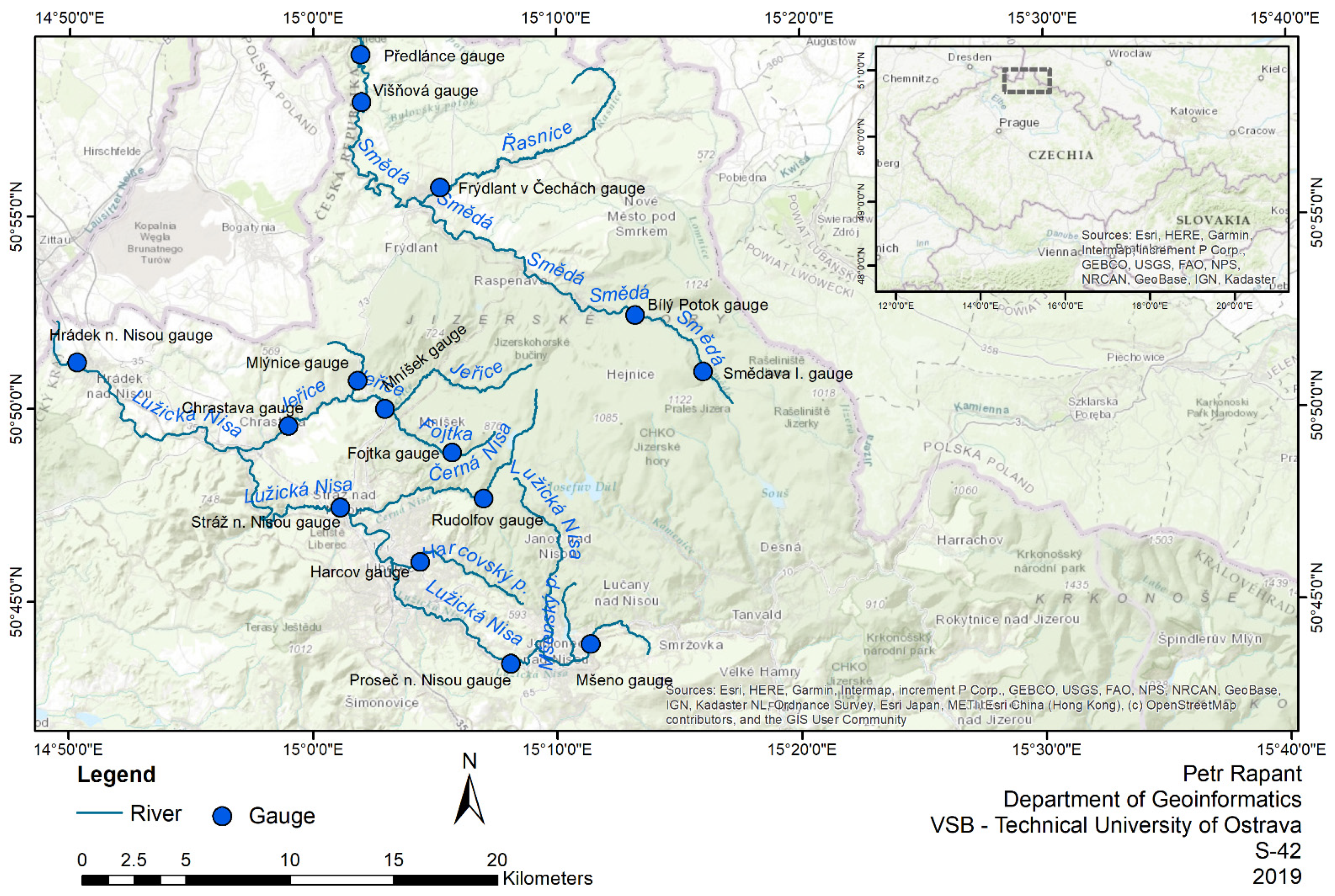
4.1.2. The Frýdlantský Spur Area
Due to the uniqueness of the two rainfall episodes hitting Northern Bohemia on 7 August 2010, we decided to investigate whether our proposed methodology would also be able, in this case, to issue an early warning before a flood hits this area. This event occurred in the two adjacent catchments with similar characteristics: that of the river Lužická Nisa and the river Smědá [83]—see Figure A1 in Appendix A. At the time of the studied episodes, both catchments were fully saturated by the preceding rainfalls.
Data on the real river flow from the hydrometric stations operated by the CHMI or Labe River Basin Management Company, a state enterprise, were obtained to verify the results of this new methodology. Using these data, we selected the hydrometric stations Chrastava on the river Jeřice, Hrádek nad Nisou on the river Lužická Nisa, and Višňová on the river Smědá, which the CHMI manages, and compared them with the respective leading edges of the forecasted flash flooding hazard. We again transformed the leading edges in each graph into normalised values between 0 and 1.
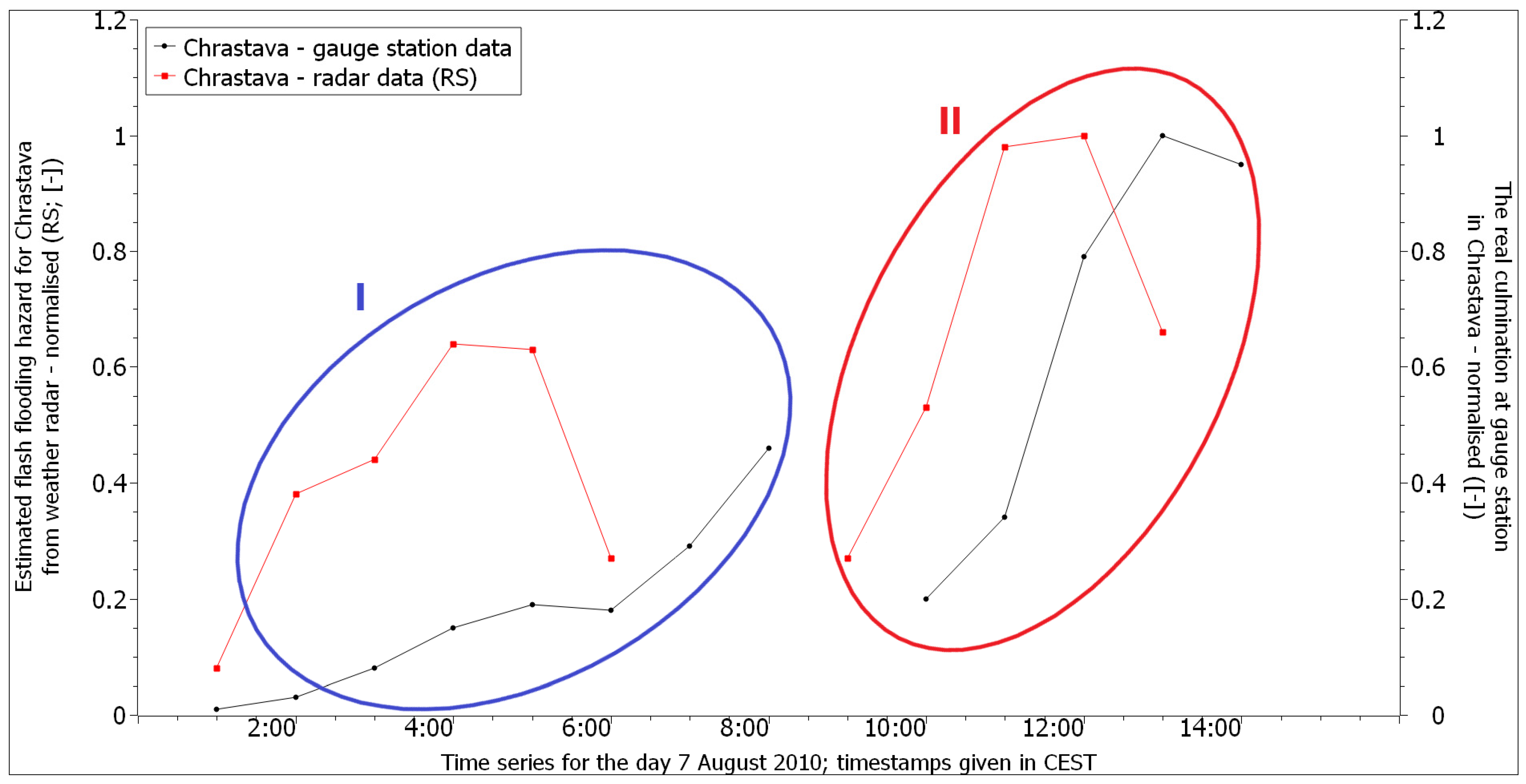
Figure A2 compares the predicted leading edges of a flash flooding hazard with the actual flow measurements at the hydrometric station Chrastava on the river Jeřice. This hydrometric station is located at the confluence of the Jeřice River and the Lužická Nisa River. The predicted leading edge precedes the actual flow leading edge by three hours in rainfall episode I and two hours in the case of rainfall episode II—see Table A1.
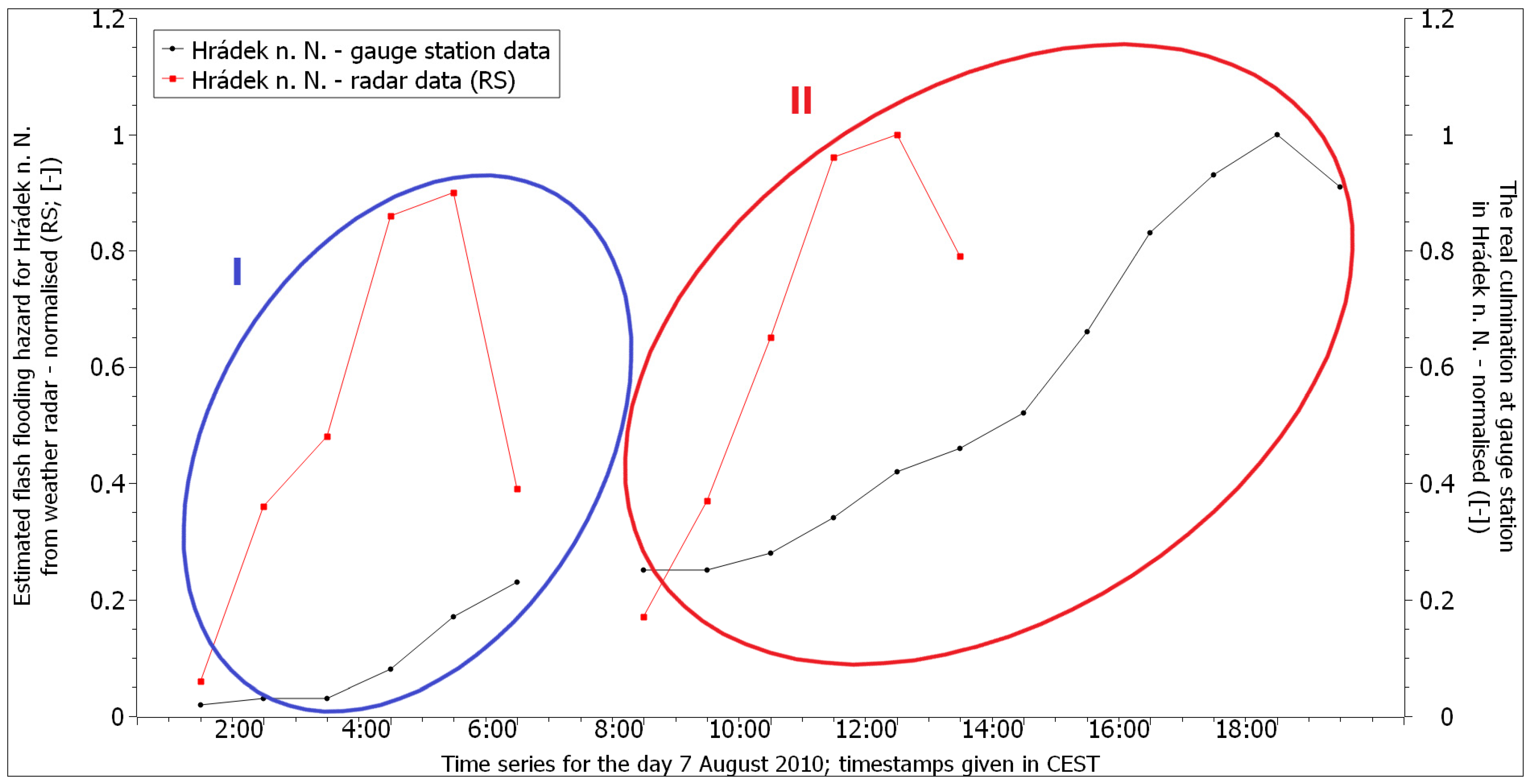
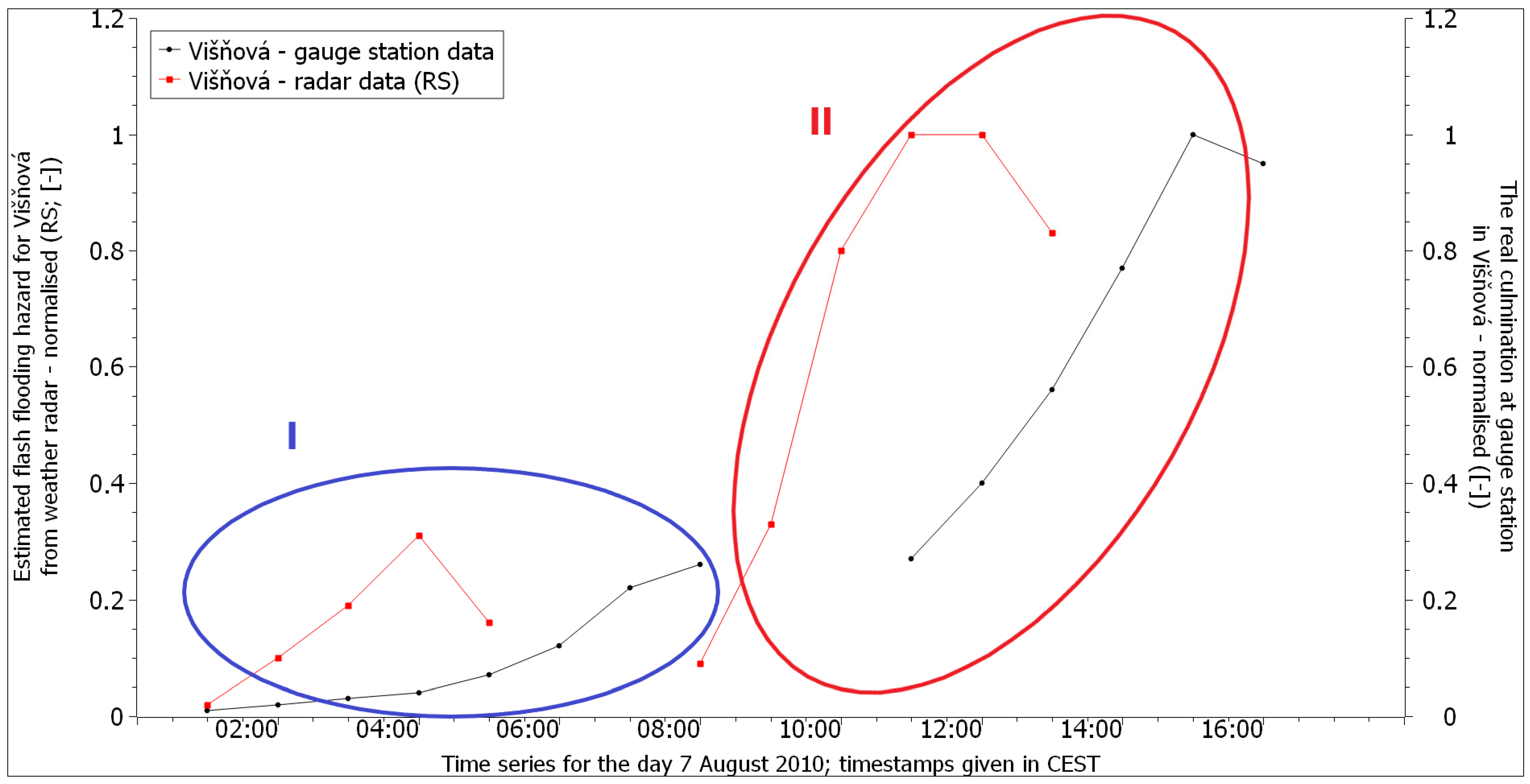
In Figure A3 and Figure A4, the leading edges are compared at the hydrometric stations Hrádek nad Nisou on the Lužická Nisa River and Višňová on the Smědá River. Again, we can see a noticeable lead time in the forecasted leading edges compared to the actual flow (three hours for the first rainfall episode and six hours for the second rainfall episode for Hrádek nad Nisou—see Table A2—and four hours for both rainfall episodes for Višňová—see Table A3). Differences in the lead times were due to the different distance between the hydrometric stations and the area affected by the heavy rainfall.
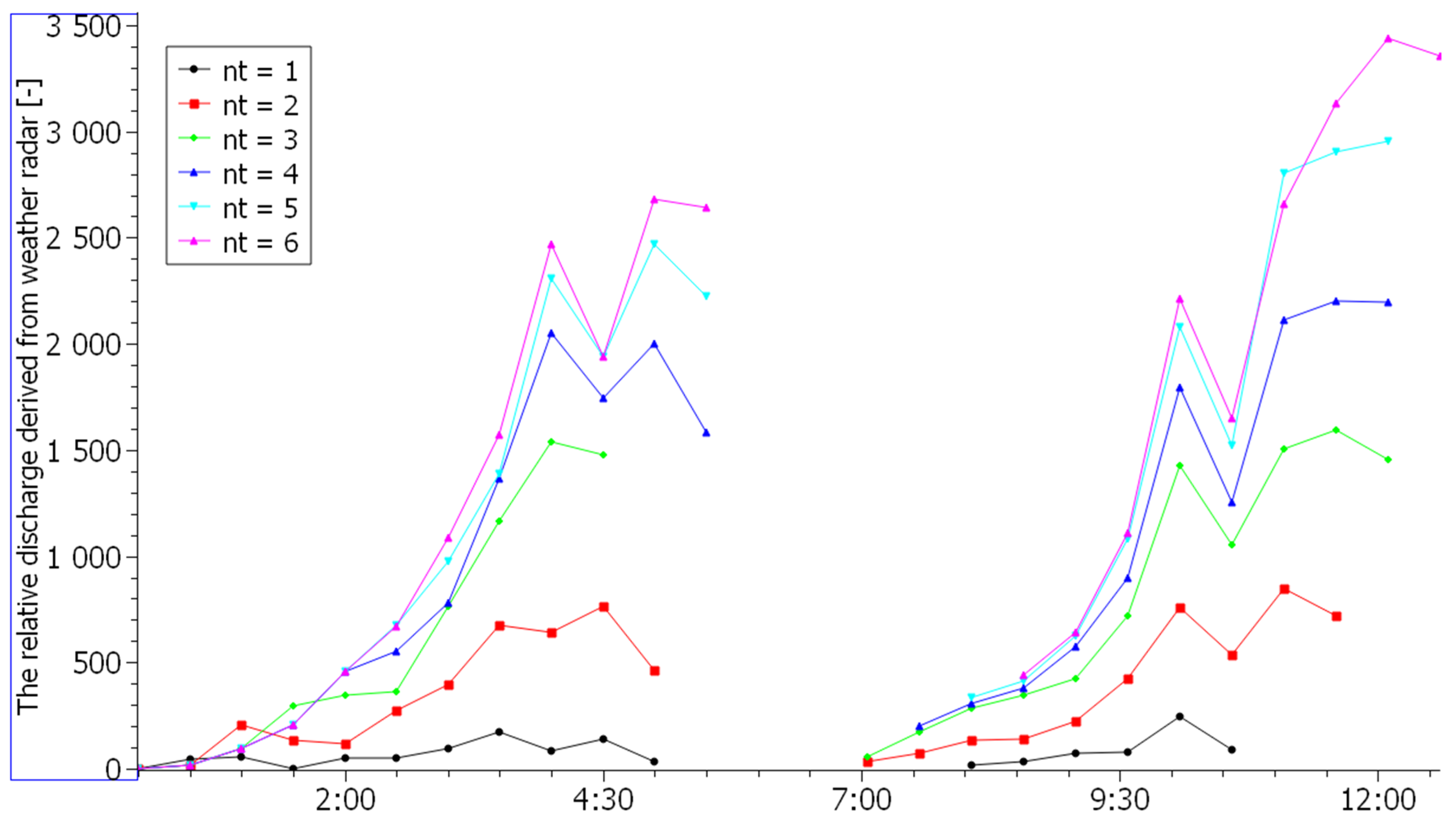
4.2. Sensitivity Testing
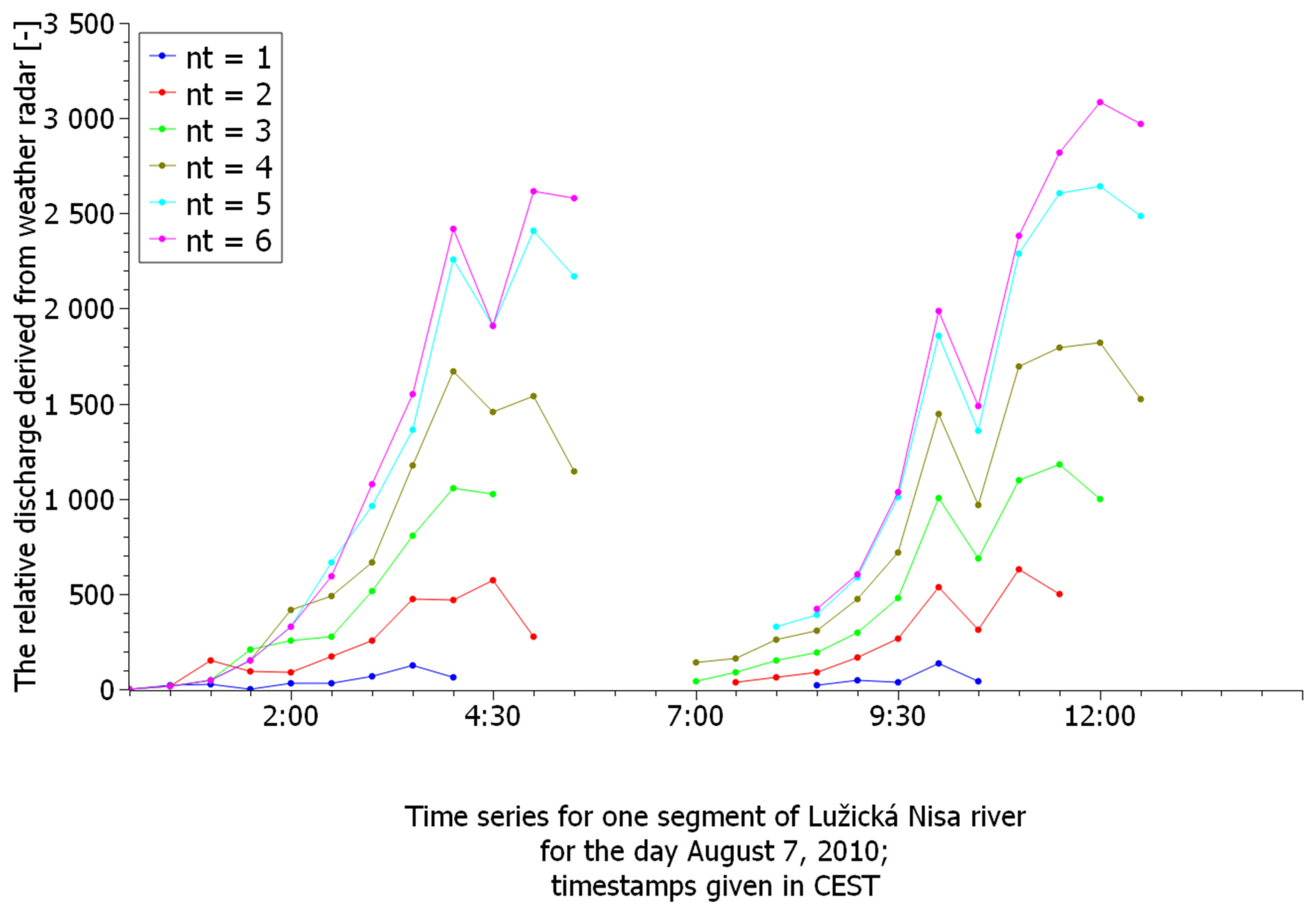
The method developed to predict the flash flooding hazard abstracts entirely from the properties of sub-watersheds and watercourses. The method has only two parameters whose values can affect the forecast. These parameters include the outflow velocity in the channel, vw, and the number of the basic time steps, nt, in which precipitation may flow to the assessed section of the watercourse. The purpose of sensitivity testing is to verify how the leading edge prediction of the flash flooding hazard is sensitive to the change in these parameters. These parameters were set to vw = 10 km/h and nt = 4 (i.e., 2 h) for routine processing. To verify the extent to which these values affect the prediction results, we conducted repeated tests in which vw was set to 10 or 15 km/h and nt varied from 1 to 6.
The testing was performed using data from the rainfall episodes on 7 August 2010. We repeatedly calculated the flash flooding hazard for watercourses in this area. We obtained two sets of six curves for each section of the watercourse that described the potential flash flooding hazard. In Figure 8, the curves are shown for vw = 10 km/h and nt = 1 to 6, and Figure 9 shows the curves for vw = 15 km/h and nt = 1 to 6. A comparison of all curves from both figures shows that the leading edges change only slightly. While intending to obtain warning information, it is essential that these leading edges of the predicted curves do not move in time, especially for nt > 2.
The third curve from the top in Figure 8 corresponds to the standard values used for both parameters in our tests.
4.3. Reliability Testing on a National Scale
The first reliability tests were carried out on a local scale. They indicated that our method produces good results under the given conditions (all watersheds were saturated—see Section 4.1). Subsequent reliability tests checked the applicability of this procedure at a national scale.
Due to its simplicity, the developed method can be easily applied to the whole country. Therefore, we decided to forecast flash flooding hazard throughout the country and compare these forecasts with data describing the real occurrence of flash floods. These data were obtained from an independent source—the official database of statistical tracking of events managed by the Fire Rescue Service of the Czech Republic. The comparison includes episodes from 10–11 June 2013 and 27 May 2014.
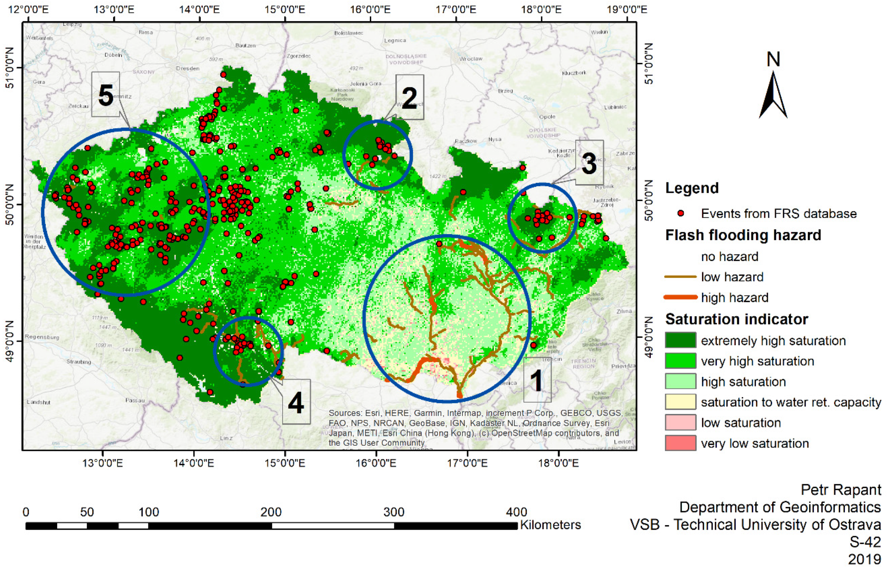
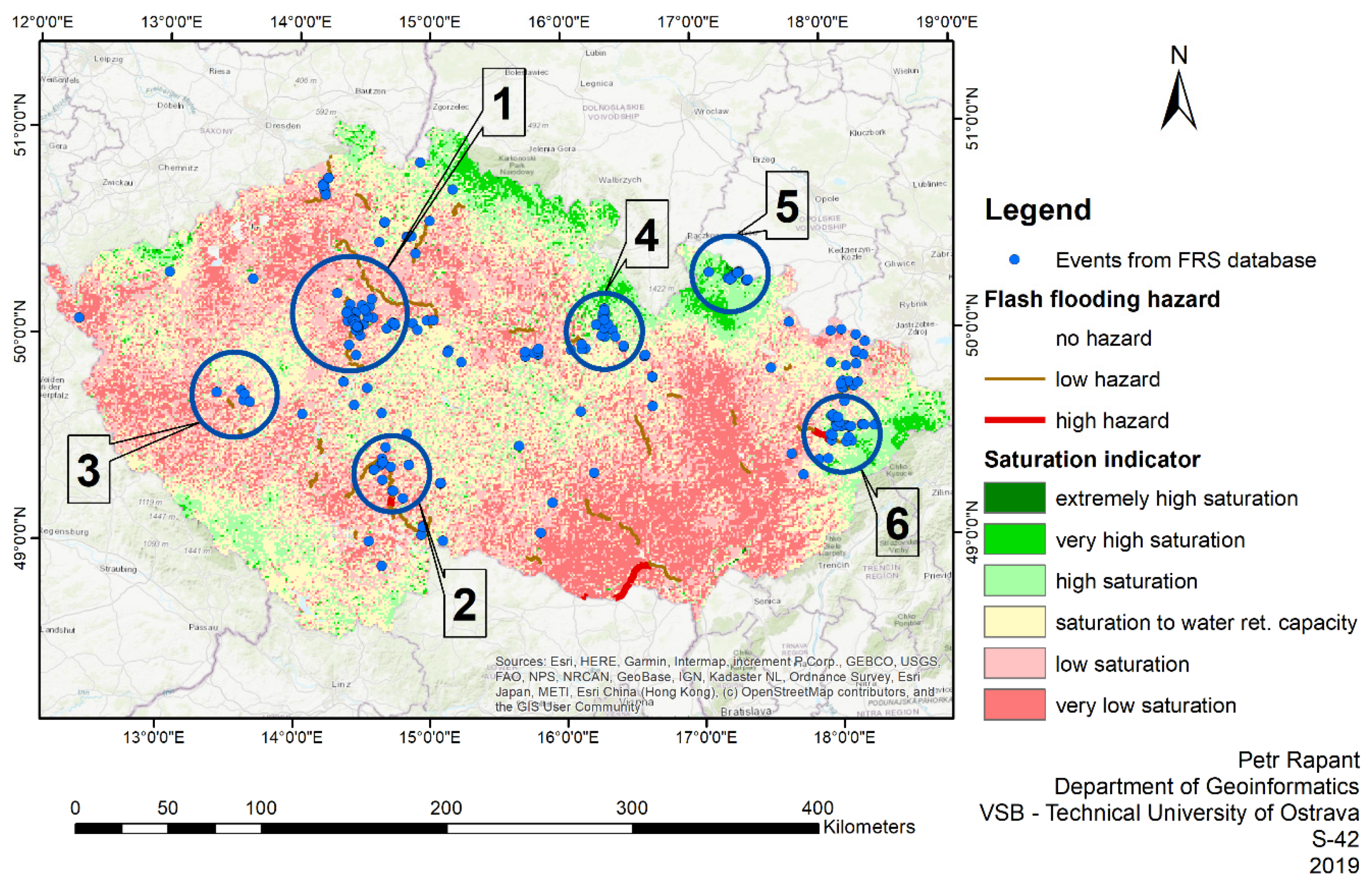
Figure 2 shows the comparison between the predicted level of the flash flooding hazard in individual sections of watercourses, the saturation indicator for 10 June 2013, 08:00 CEST provided by CHMI, and the events related to Fire Rescue Service interventions between 10 June 2013, 12:00 CEST and 11 June 2013, 11:55 CEST.
Figure 2 shows the following:
- During that period, the soils throughout the Czech Republic were saturated to extremely saturated;
- Most of the rainfall and the highest predicted hazard values occur in the south-eastern part of the Czech Republic, which has the lowest value of the saturation indicator; in this region, there is almost zero incidence of Fire Rescue Service interventions due to flooding (area 1), although the area is densely populated;
- There is a correlation between the occurrence of an increased flash flooding hazard, high values of the saturation indicator, and a higher incidence of Fire Rescue Service interventions due to floods (areas 2, 3, and 4);
- An increased incidence of Fire Rescue Service interventions occurs in an area not forecasted to be possibly endangered by an increased flash flooding hazard. Still, there are high values of the saturation indicator (area 5). A detailed examination reveals that the bulk of the interventions concentrate on brooks for which the suggested procedure is not intended.
Figure 10 shows the comparison between the maximum predicted level of the flash flooding hazard for individual sections of watercourses, the saturation indicator on 27 May 2014, 08:00 CEST, and the interventions of the Fire Rescue Service due to floods on 27 May 2014, between 00:00 CEST and 23:55 CEST.
Figure 10 shows the following:
- Soils throughout the Czech Republic were low saturated (in the lowlands and uplands) to high saturated (in mountain areas);
- Most of the rainfall and the highest predicted hazard values occur coincidentally in areas with the lowest values of the saturation indicator; there are almost zero incidence of Fire Rescue Service interventions due to flooding in these areas. Exceptions include area 1, located in the city of Prague—a heavily urbanised region—and areas 2 and 3, where the Fire Rescue Service interventions are mostly bound to the municipality not situated nearby watercourses (i.e., again events tied to urbanised areas); only part of the interventions was done near rivers;
- There is a correlation between an increased flash flooding hazard, higher values of the saturation indicator, and a higher incidence of Fire Rescue Service interventions due to flooding (areas 4, 5, and 6).
5. Discussion
Braud et al. [28] identified some difficulties of flash flood forecasting. Among others, they mentioned that flash floods hit mostly small, ungauged watersheds. This situation results in a lack of discharge observations, so no data support the development and calibration of hydrological models. The other problem is that watersheds respond to heavy rainfall very quickly. Hence, the flash flooding hazard forecast method must be rapid enough to provide a leading time sufficient to warn people. High precipitation intensity and large discharges can lead modellers to excessive simplification of the model, most often assuming that all precipitation flows into watercourses. The result is a high rate of false warnings.
The proposed methodology is not based on a hydrological model, so we need no data from hydrometric gauge stations for model calibration. That is why our method is suitable even for ungauged watersheds. The method uses as simple data collection and processing as possible, and so it provides adequate leading time from tens of minutes up to some hours. On the other hand, the basic version of this method envisages the worst-case scenario, i.e., that all precipitation flows into the watercourse. If this method was used for fully saturated watersheds, the results obtained were in good agreement with reality.
However, when the method was applied under normal conditions, false positives were generated to an increased extent. Nevertheless, if the method was supplemented by the saturation indicator, which made it possible to reduce the runoff from low-saturated areas significantly, there was a noteworthy reduction in false alarms. The extended method, therefore, gives good results even in unsaturated areas.
For the needs of timely early warning on the onset of a flash flood, Tsai et al. [86] identified the main factors in evaluating methods of flash flood forecast as the lead time, flood forecast accuracy, and the proportion of manual processing. It is ideal to have the forecast available continuously in real-time, but for practical reasons, a more commonly used step of flood hazard assessment is 10 min. The resulting warning information must be presented effectively, i.e., the warning should be targeted only at truly endangered areas.
The authors in [87] mention that the minimum lead time of flood warning acceptable by the population at risk is two hours. The lead time provided by the proposed method spans from tens of minutes to some hours. The flash flooding hazard forecast is offered in half-hour steps. This time step was chosen as a reasonable compromise between the forecast speed and results reliability. The method is based on the processing of uncertain raw weather radar data. Their uncertainty is reduced to some extent by the sum of six consecutive radar records. In addition, these predictions are not related to vast areas such as counties but segments of watercourses. This approach allows for issuing a warning only to the genuinely endangered municipalities.
The ability to issue early warnings of flash floods requires predicting future flow rates in vulnerable river basins [88]. These predictions must be available with a lead time that allows for the early warning of the population to leave the endangered area safely. There is no time for implementing preventive measures, such as the construction of flood defences, etc., in flash floods. Therefore, ways are being sought to prolong the lead time of flash floods, for example, by using precipitation prediction. The quality of flood forecasting based on a hydrological model depends mainly on the precipitation measurement and nowcasting quality. It also depends on the speed at which this nowcasting can be made. We decided not to use precipitation predictions and hydrological models. Our methodology provides less precise (both in time and space dimensions) forecasts but with a longer lead time.
The success of the early warning method can be evaluated, for example, using the critical success index [11]:
CSI = true alarms/(true alarms + missed alarms + false alarms)
A CSI value of 1.0 means full success, while a value of 0.0 means a total lack of skill. The problem is how to define the spatial unit, for which we will classify alarms. For example, in the proposed methodology, a watercourse segment seems to be a natural spatial unit. We should collect data about flash flood occurrence for every watercourse segment to evaluate the flash flooding hazard forecast utility. However, obtaining such data without extensive fieldwork is quite challenging. Moreover, it is impossible to collect such data afterwards. For this reason, assessing of performance of the system for flash flooding hazard forecasting for ungauged watersheds is challenging [89].
The success of the proposed method depends on the soil moisture conditions of the watershed. In the case of local testing sites (Novojičínsko and Frýdlantský Spur Area), we saw that the method was quite successful. Due to fully saturated soils in both regions, the worst-case scenario adopted by the proposed method was adequate. On the other hand, both national-level examples demonstrated that this is not always the case. Nevertheless, prediction success could be raised substantially when the saturation indicator is included in the developed method.
According to Lincoln [90], despite the possibility of less accurate identification of flash floods (both in space and time) and a higher number of false alarms, a system using uncorrected radar precipitation estimates was considered more valuable by river basin management operators than a system based on adjusted radar precipitation estimates. The update time of the first system was much shorter (5 min in the best case) than the second one (30 to 90 min), thus speeding up decision-makers’ response. Furthermore, any method used for early warning of flash floods should include routing runoff to downstream sites. Some severe flash flood impacts are recorded downstream of the place where runoff is generated; in some cases even outside the precipitation area [90]. Our results from both local flash flooding sites comply with these conclusions, and thus, also with the developed method.
Any early warning method faces how to determine the threshold above which an alert can be issued. It does not matter whether the amount of channel discharge or just the level of the flash flooding hazard is evaluated. There are several approaches to solving this problem. The FFG method, for example, determines the intensity of rainfall, which, if it lasts three hours, will cause the overflow of banks of the watercourses. According to Llort et al. [91], the decision as to whether the flash flood is expected to occur in a river basin can be made based on an assessment of the exceedance of the threshold value of the anticipated maximum precipitation accumulation value. This value can be determined by the frequency analysis of historical rainfall data. Zanchetta and Coulibaly [11] proposed comparing channel discharge with Tresh-R values. For gauged watersheds for which a reliable rating curve is available, the bank full water level values can be used as the Thresh-R [92]. Hapuarachchi in [62] recommended a similar approach. For ungauged watersheds, Thresh-R values can be estimated by simulation of the flow [76]. Another method, recommended by Zanchetta and Coulibaly [11], is based on deep learning techniques. This method has shown promising results but is still under development. There is a discussion about some of the issues related to validation metrics and the size of training datasets.
Deep learning techniques build on the analysis of long time series. In the case of flash floods, the methods quickly encounter a problem: while estimates of radar precipitation are collected over a long period of time and with sufficient spatial and temporal detail, contrary to this, discharge is also registered for a long time, but only in a minimal number of places. Thus, the data provide great time detail but are very sparse in the spatial domain. From this point of view, deep learning methods to flash flooding hazard forecasting are pretty challenging. We plan to combine this approach with our methodology. The proposed method will be used to calculate the flash flooding hazard value, and a deep learning technique, probably an artificial neural network, will be used to classify the flash flooding hazard level at watercourse segments. It will be re-trained after every event based on the known impacts of that event. We suppose that this approach can improve the reliability of early flash flooding warnings.
The authors in [88,93] and others mentioned Transfer Function Models. These models forecast river flows using current and previous observations of rainfall and previous observations of flow. Forecast values are derived from these data only, so they do not need any details on watersheds. These models are some kind of black-box models. The method is very robust and fast and can be run in real-time. It applies to watersheds with rainfall-runoff time series data available to infer watersheds transfer function transforming rainfall to runoff. The result of these models is presented as a hydrogram.
To some extent, our approach is similar. The main difference is that we have no time series of runoff, so our transformation of rainfall to potential runoff cannot deal with time delays in the outflow. As a result, the output of our method cannot be presented as the hydrogram but only as a prediction of potential hazard in the near future.
Meteo-France is running an automated flash flooding warning system based on the AIGA (Adaptation d’Information Géographique pour l’Alerte en Crue) method [89,94], which covers ungauged watersheds greater than 10 square kilometres and has a response time longer than one and a half hours [38]. The AIGA method is based on a simplified distributed rainfall-runoff model. It compares the currently modelled discharges with reference flood quantiles obtained by modelling and continuous re-analysis of radar-gauge rainfall. Two warning levels are taken into account: high flood and very high flood. The model is calibrated and provide outputs every 15 min. This system is designed for and run over the area well monitored by meteorological service. Although the method we have proposed is very similar to the Meteo-France approach, it differs from it in terms of data complexity and the absence of a hydrological model.
Evolving early warning systems for urban areas work with very detailed data—with a spatial resolution of up to 1 square kilometre and a temporal resolution of up to 5 min [34,35]. As input, they use weather radar, rain gauge statins, nowcasting, and a detailed description of the urban environment to prepare predictions using very detailed hydraulic and hydrological models. The result predicts the hazard of flash floods, which can be used to manage the crisis in cities. From the point of view of spatial resolution and detailed data and models, it differs significantly from the proposed method. As already mentioned, it is intended primarily for areas with minimal data sources, where it is not possible to process and operate a quality hydrological and hydraulic model. For an urban environment, it is challenging to derive a drainage network without a detailed digital terrain or surface model. Therefore, the proposed method is not suitable for such an environment.
Early warning systems often use data from nowcasting as input. The proposed method uses raw weather radar data only. Nowcasting was not included in the method because it uses weather radar and rain gauge stations, wind profiler, and other weather data and numerical weather prediction models [35]. Thus, if nowcasting is available for the monitored area, more comprehensive tools for flash flooding hazard forecasting will probably be used. The proposed method can be used as a “first-guess early warning” only in such a situation.
On the other hand, nothing prevents the use of nowcasting in our method. If we use data from nowcasting instead of radar data as input, the method will work the same. The benefit would be that nowcasting will allow extending the lead time of warning against a potential increase in flash flooding hazard.
As for the quality of weather radar data, their increasing accuracy and reliability will naturally lead to improved accuracy and reliability of the outputs of the proposed method.
The method uses two parameters: the outflow velocity in the channel, vw, and the number of the basic time steps, nt, in which precipitation may flow to the assessed section of the watercourse. The operator can set both parameters. These parameters control the distance to which rainfall will travel through watercourse segments in the evaluated time interval. We used values vw = 10 km/h and nt = 4. This means that every watercourse segment can receive outflow from a distance up to 20 km upstream from the last two hours in the current time. Sensitivity analysis showed that these parameters influence the leading edge height only, but its position in time is independent for an evaluated time interval longer than 1 h. If limits for hazard evaluation will be derived using machine learning, these parameters should be set at the beginning of monitoring an area and should not be changed later.
Sensitivity analysis discussed parameters of the method only. Of course, the method is also sensitive to uncertainties hidden in radar data. The authors in [95] showed that radar precipitation estimates tend to underestimate intensive precipitation based on the evaluation of specific events in the territory of four different states. In the case of the proposed method, this means that it will underestimate the flash flooding hazard. In practice, this would mean fewer positive warnings issued to citizens. However, if an artificial neural network will be used for the flash flooding hazard level evaluation, it will probably decrease the impact of this underestimation after some time due to periodic re-training.
6. Conclusions
The procedure currently used for the prediction of heavy rainfall and the resulting flash floods generally require quantitative data, such as the soil saturation of the territory by previous rainfall, radar estimates of rainfall in millimetres, detailed characteristics of the basin, and, if possible, continuous evaluation of the predictions using the results of hydrometric gauge stations located on the watercourse network. Therefore, these procedures are dependent on a large amount of input data that is not always available.
From this perspective, the proposed method is less data-intensive. It does not rely on an on-ground monitoring network or hydrological models. It is, therefore, suitable for less developed areas, covered only by weather radar. It is much simpler and operational but only allows for a qualitative prediction of the flash flooding hazard so that only an early warning of growing flash flooding hazard can be issued and does not include any quantified estimates of the impact (e.g., exact time of flash flooding, delimitation of potentially flooded areas). However, a fast warning to residents will give them a chance to move quickly to a safer location at a higher altitude in their vicinity.
Simply speaking, the proposed procedure does a straightforward transformation: in the input, we have a 2D signal carrying information about the spatial and temporal distribution of precipitation over some territory recorded by the weather radar, and we transform it, using sub-watershed and watercourse networks, to “concentrated” 1D signal related to sections of watercourses and describing potential runoff along them. If the strength of the 1D signal is very high at some watercourse segment, we can issue a warning of possible flash flooding to nearby municipalities. If the preceding rainfall well saturates soils over the hit territory, the method works quite well. In other cases, the method can generate too many false alarms. The rate of false alarms can be reduced substantially by including the saturation indicator. Alternatively, we tried to use the sum of radar reflections for the last seven days instead of the saturation indicator. The results were promising, but more research is needed on this option.
Due to low data requirements, this procedure can be easily applied to areas with undeveloped monitoring infrastructure. Practical offline tests confirmed the effectiveness and efficiency of this proposed method to predict flash flooding hazard.
Author Contributions
Conceptualisation, P.R.; Methodology, P.R. and J.K.; Software, P.R.; Validation, P.R.; Formal Analysis, P.R. and J.K.; Investigation, P.R. and J.K.; Resources, P.R.; Data Curation, P.R.; Writing—Original Draft Preparation, P.R. and J.K.; Writing—Review and Editing, P.R.; Visualisation, P.R.; Supervision, P.R.; Project Administration, P.R.; Funding Acquisition, P.R. and J.K. All authors have read and agreed to the published version of the manuscript.
Funding
This work was supported by the project called “Disaster management support scenarios using geoinformation technologies” No VG20132015106, program Safety Research promoted by the Ministry of Interior, the Czech Republic and by the Faculty of Mining and Geology, VSB—Technical University of Ostrava, the Czech Republic.
Institutional Review Board Statement
Not applicable.
Informed Consent Statement
Not applicable.
Data Availability Statement
Data on hydrological division and stream network can be downloaded from website https://www.dibavod.cz/index.php?id=27 (accessed on 26 July 2021). Weather radar data and saturation indicator can be obtained from the Czech Hydro-Meteorological Institute (https://www.chmi.cz/ (accessed on 26 July 2021)). Data from hydro-metric stations can be obtained from the Czech Hydro-Meteorological Institute (https://www.chmi.cz/ (accessed on 26 July 2021)), Odra River Basin Management Company, state enterprise (https://www.pod.cz/ (accessed on 26 July 2021)) and Labe River Basin Management Company, state enterprise (http://www.pla.cz/planet/webportal/internet/default.aspx (accessed on 26 July 2021)).
Conflicts of Interest
The authors declare no conflict of interest.
Appendix A
Figures and tables for the Frýdlant spur area.
Figure A1.
The Frýdlant spur area with hydrometric gauge stations.

Figure A2.
Comparison of the leading edges of the normalised flow measured at a professional gauge station with the leading edges of the normalised forecasted flash flooding risk derived from radar data for the profile Chrastava on the river Jeřice (I—the leading edges for rainfall episode I; II—the leading edges for rainfall episode II).


Table A1.
The cross-correlation calculated between the curves from Figure A2.
Table A1.
The cross-correlation calculated between the curves from Figure A2.
| Rainfall Episode I | ||||||
| Shift [h] | 0 | 1 | 2 | 3 | 4 | 5 |
| Cross-correlation [-] | 0.616 | 0.388 | 0.140 | 0.752 | 0.624 | −0.015 |
| Rainfall Episode II | ||||||
| Shift [h] | 0 | 1 | 2 | 3 | 4 | 5 |
| Cross-correlation [-] | 0.432 | 0.840 | 0.906 | 0.376 | −0.555 | −0.587 |
Figure A3.
Comparison of the leading edges of the normalised flow measured at a professional gauge station with the leading edges of the normalised forecasted flash flooding risk derived from radar data for the profile Hrádek nad Nisou on the river Lužická Nisa (I—leading edges for rainfall episode I; II—leading edges for rainfall episode II).

Table A2.
The cross-correlation calculated between the curves from Figure A3.
Table A2.
The cross-correlation calculated between the curves from Figure A3.
| Rainfall Episode I | ||||||||
| Shift [h] | 0 | 1 | 2 | 3 | 4 | 5 | 6 | 7 |
| Cross-correlation [-] | 0.384 | 0.643 | 0.775 | 0.790 | 0.645 | 0.149 | 0.232 | 0.507 |
| Rainfall Episode II | ||||||||
| Shift [h] | 0 | 1 | 2 | 3 | 4 | 5 | 6 | 7 |
| Cross-correlation [-] | 0.801 | 0.884 | 0.829 | 0.783 | 0.849 | 0.924 | 0.989 | 0.785 |
Figure A4.
Comparison of the leading edges of the normalised flow measured at a professional gauge station with the leading edges of the normalised forecasted flash flooding risk derived from radar data for the profile Višňová on the river Smědá (adopted from [84]) (I—leading edges for rainfall episode I; II—leading edges for rainfall episode II).

Table A3.
The cross-correlation calculated between the curves from Figure A4.
Table A3.
The cross-correlation calculated between the curves from Figure A4.
| Rainfall Episode I | |||||||
| Shift [h] | 0 | 1 | 2 | 3 | 4 | 5 | 6 |
| Cross-correlation [-] | 0.599 | 0.480 | 0.441 | 0.719 | 0.975 | 0.946 | 0.061 |
| Rainfall Episode II | |||||||
| Shift [h] | 0 | 1 | 2 | 3 | 4 | 5 | 6 |
| Cross-correlation [-] | 0.392 | 0.012 | 0.606 | 0.889 | 0.962 | 0.472 | −0.474 |
References
- Gaume, E.; Bain, V.; Bernardara, P.; Newinger, O.; Barbuc, M.; Bateman, A.; Blaškovičová, L.; Blöschl, G.; Borga, M.; Dumitrescu, A.; et al. A compilation of data on European flash floods. J. Hydrol. 2009, 367, 70–78. [Google Scholar] [CrossRef] [Green Version]
- Marchi, L.; Borga, M.; Preciso, E.; Gaume, E. Characterisation of selected extreme flash floods in Europe and implications for flood risk management. J. Hydrol. 2010, 394, 118–133. [Google Scholar] [CrossRef]
- Norbiato, D.; Borga, M.; Degli Esposti, S.; Gaume, E.; Anquetin, S. Flash flood warning based on rainfall thresholds and soil moisture conditions: An assessment for gauged and ungauged basins. J. Hydrol. 2008, 362, 274–290. [Google Scholar] [CrossRef]
- Borga, M.; Gaume, E.; Creutin, J.; Marchi, L. Surveying flash floods: Gauging the ungauged extremes. Hydrol. Process. 2008, 22, 3883–3885. [Google Scholar] [CrossRef]
- Borga, M.; Boscolo, P.; Zanon, F.; Sangati, M. Hydrometeorological Analysis of the 29 August 2003 Flash Flood in the Eastern Italian Alps. J. Hydrometeorol. 2007, 8, 1049–1067. [Google Scholar] [CrossRef]
- Collier, C. Flash flood forecasting: What are the limits of predictability? Q. J. R. Meteorol. Soc. 2007, 133, 3–23. [Google Scholar] [CrossRef]
- Corral, C.; Berenguer, M.; Sempere-Torres, D.; Poletti, L.; Silvestro, F.; Rebora, N. Comparison of two early warning systems for regional flash flood hazard forecasting. J. Hydrol. 2019, 572, 603–619. [Google Scholar] [CrossRef] [Green Version]
- Jonkman, S. Global Perspectives on Loss of Human Life Caused by Floods. Nat. Hazards 2005, 34, 151–175. [Google Scholar] [CrossRef]
- World Meteorological Organization (WMO). Manual on Flood Forecasting and Warning; WMO-No. 1072; World Meteorological Organization: Geneva, Switzerland, 2011. [Google Scholar]
- Borga, M.; Anagnostou, E.; Blöschl, G.; Creutin, J. Flash flood forecasting, warning and risk management: The HYDRATE project. Environ. Sci. Policy 2011, 14, 834–844. [Google Scholar] [CrossRef]
- Zanchetta, A.; Coulibaly, P. Recent Advances in Real-Time Pluvial Flash Flood Forecasting. Water 2020, 12, 570. [Google Scholar] [CrossRef] [Green Version]
- Solomatine, D.; Ostfeld, A. Data-driven modelling: Some past experiences and new approaches. J. Hydroinform. 2008, 10, 3–22. [Google Scholar] [CrossRef] [Green Version]
- Ticlavilca, A.; Torres, A. Data Driven Models and Machine Learning Approach in Water Resources Systems: Guest Lecture. In Proceedings of the Water Resources System Analysis; Utah State University: Logan, Utah, 2012; pp. 1–18. [Google Scholar]
- See, L.; Solomatine, D.; Abrahart, R.; Toth, E. Hydroinformatics: Computational intelligence and technological developments in water science applications—Editorial. Hydrol. Sci. J. 2007, 52, 391–396. [Google Scholar] [CrossRef] [Green Version]
- Jain, S.K.; Mani, P.; Jain, S.K.; Prakash, P.; Singh, V.P.; Tullos, D.; Kumar, S.; Agarwal, S.P.; Dimri, A.P. A Brief review of floodforecasting techniques and their applications. Int. J. River Basin Manag. 2018, 16, 329–344. [Google Scholar] [CrossRef]
- Janál, P. Flash Floods Forecasting—Fuzzy Model. In Proceedings of the Hospodaření s Vodou v Krajině, Třeboň, The Czech Republic, 21–22 June 2018; pp. 1–10. Available online: http://cbks.cz/SbornikTrebon18/Janal.pdf (accessed on 26 July 2021).
- Modrick, T.; Graham, R.; Shamir, E.; Jubach, R.; Spencer, C.; Sperfslage, J.; Georgakakos, K. Operational flash flood warning systems with global applicability. In Proceedings of the 7th International Congress on Environmental Modelling and Software, San Diego, CA, USA, 15–19 June 2014; pp. 1–8. [Google Scholar]
- Surface Water Management. An Action Plan. Department for Environment, Food & Rural Affairs. 2018; 41p. Available online: https://assets.publishing.service.gov.uk/government/uploads/system/uploads/attachment_data/file/725664/surface-water-management-action-plan-july-2018.pdf (accessed on 2 July 2021).
- Ochoa-Rodríguez, S.; Wang, L.; Thraves, L.; Johnston, A.; Onof, C. Surface water flood warnings in England: Overview, assessmentand recommendations. J. Flood Risk Manag. 2015, S211. [Google Scholar] [CrossRef]
- Gaume, E. Post Flash-flood Investigations—Methodological Note; FLOODsite: Wallingford, UK, 2006. [Google Scholar]
- Koutroulis, A.; Tsanis, I. A method for estimating flash flood peak discharge in a poorly gauged basin: Case study for the 13–14 January 1994 flood, Giofiros basin, Crete, Greece. J. Hydrol. 2010, 385, 150–164. [Google Scholar] [CrossRef]
- Wharton, G. Flood estimation from channel size: Guidelines for using the channel-geometry method. Appl. Geogr. 1992, 12, 339–359. [Google Scholar] [CrossRef]
- Wharton, G.; Arnell, N.; Gregory, K.; Gurnell, A. River discharge estimated from channel dimensions. J. Hydrol. 1989, 106, 365–376. [Google Scholar] [CrossRef]
- Dorman, L. Automated Local Evaluation in Real Time (ALERT). In Encyclopedia of Natural Hazards; Bobrowsky, P., Ed.; Encyclopedia of Earth Sciences Series; Springer: Dordrecht, The Netherlands, 2013; p. 31. ISBN 978-90-481-8699-0. [Google Scholar]
- Georgakakos, K. On the design of national, real time warning systems with capability for se-specific flash flood forecasts. Bull. Am. Meteorol. Soc. 1986, 67, 1233–1239. [Google Scholar] [CrossRef]
- Grabs, W. Regional Flash Flood Guidance and Early Warning System. In Proceedings of the Training for Trainers. Workshop on Integrated Approach to Flash Flood and Flood Risk Management, Kathmandu, Nepal, 25 October–2 November 2010; pp. 24–28. [Google Scholar]
- Braud, I.; Vincendon, B.; Anquetin, S.; Ducrocq, V.; Creutin, J. The Challenges of Flash Flood Forecasting. In Mobilities Facing Hydrometeorological Extreme Events 1; Elsevier: Amsterdam, The Netherlands, 2018; pp. 63–88. ISBN 9781785482892. [Google Scholar]
- Alfieri, L.; Smith, P.; Thielen-del Pozo, J.; Beven, K. A staggered approach to flash flood forecasting—Case study in the Cévennes region. Adv. Geosci. 2011, 29, 13–20. [Google Scholar] [CrossRef] [Green Version]
- COSMO: Consortium for Small-Scale Modeling. Available online: http://www.cosmo-model.org/ (accessed on 19 July 2020).
- Panziera, L.; Gabella, M.; Zanini, S.; Hering, A.; Germann, U.; Berne, A. A radar-based regional extreme rainfall analysis to derive the thresholds for a novel automatic alert system in Switzerland. Hydrol. Earth Syst. Sci. 2016, 20, 2317–2332. [Google Scholar] [CrossRef] [Green Version]
- Liechti, K.; Panziera, L.; Germann, U.; Zappa, M. The potential of radar-based ensemble forecasts for flash-flood early warning in the southern Swiss Alps. Hydrol. Earth Syst. Sci. 2013, 17, 3853–3869. [Google Scholar] [CrossRef] [Green Version]
- Thielen, J.; Bartholmes, J.; Ramos, M.; de Roo, A. The European Flood Alert System—Part 1: Concept and development. Hydrol. Earth Syst. Sci. 2009, 13, 125–140. [Google Scholar] [CrossRef] [Green Version]
- Park, S.; Berenguer, M.; Sempere-Torres, D. Long-term analysis of gauge-adjusted radar rainfall accumulations at European scale. J. Hydrol. 2019, 573, 768–777. [Google Scholar] [CrossRef] [Green Version]
- Hofmann, J.; Schuttrumpf, H. Risk-Based Early Warning System for Pluvial Flash Floods: Approaches and Foundations. Geosciences 2019, 9, 127. [Google Scholar] [CrossRef] [Green Version]
- Speight, L.J.; Cranston, M.D.; White, C.J.; Kelly, L. Operational and emerging capabilities for surface water flood forecasting. WIREs Water 2021, 8, e1517. [Google Scholar] [CrossRef]
- Ogale, S.; Srivastava, S. Modelling and Short Term Forecasting of Flash Floods in an Urban Environment. In Proceedings of the 2019 National Conference on Communications (NCC), Bangalore, India, 20–23 February 2019; Available online: https://ieeexplore.ieee.org/stamp/stamp.jsp?tp=&arnumber=8732193 (accessed on 2 July 2021).
- Bucherie, A.; Werner, M.; Homberg, M.; Tembo, S. Flash Flood warning in context: Combining local knowledge and large-scale hydro-meteorological patterns. Preprint. Nat. Hazards Earth Syst. Sci. 2021. [Google Scholar] [CrossRef]
- Javelle, P.; Saint-Martin, C.; Garandeau, L.; Janet, B. Flash Flood Warnings: Recent Achievements in France with the National Vigicrues Flash System. Contributing Paper to GAR 2019. Available online: https://www.undrr.org/publication/flash-flood-warnings-recent-achievements-france-national-vigicrues-flash-system (accessed on 2 July 2021).
- Flack, D.L.; Skinner, C.J.; Hawkness-Smith, L.; O’Donnell, G.; Thompson, R.J.; Waller, J.A.; Chen, A.S.; Moloney, J.; Largeron, C.; Xia, X.; et al. Recommendations for improving integration in National end-to-end Flood Forecasting Systems: An overview of the FFIR (flooding from intense rainfall) Programme. Water 2019, 11, 725. [Google Scholar] [CrossRef] [Green Version]
- Tucker, G.; Bras, R. Hillslope processes, drainage density, and landscape morphology. Water Resour. Res. 1998, 34, 2751–2764. [Google Scholar] [CrossRef] [Green Version]
- Seibert, J.; McDonnell, J. On the dialog between experimentalist and modeler in catchment hydrology: Use of soft data for multicriteria model calibration. Water Resour. Res. 2002, 38, 23-1–23-14. [Google Scholar] [CrossRef]
- Germann, U.; Galli, G.; Boscacci, M.; Bolliger, M. Radar precipitation measurement in a mountainous region. Q. J. R. Meteorol. Soc. 2006, 132, 1669–1692. [Google Scholar] [CrossRef]
- Use of Radio Spectrum for Meteorology: Weather, Water and Climate Monitoring and Prediction; WMO-ITU: Geneva, Switzerland, 2017; ISBN 978-92-61-24876-5.
- CHMI Úspěšná Realizace Projektu Upgrade Měřicích Systémů pro Předpovědní a Výstražnou Službu: Tisková Zpráva. Available online: https://www.chmi.cz/files/portal/docs/ruzne/Radary/radary.pdf (accessed on 26 July 2021).
- Creutin, J.; Borga, M. Radar hydrology modifies the monitoring of flash-flood hazard. Hydrol. Process. 2003, 17, 1453–1456. [Google Scholar] [CrossRef]
- Mishra, A.; Coulibaly, P. Developments in hydrometric network design: A review. Rev. Geophys. 2009, 47, RG2001. [Google Scholar] [CrossRef]
- Sieck, L.; Burges, S.; Steiner, M. Challenges in obtaining reliable measurements of point rainfall. Water Resour. Res. 2007, 43, W01420. [Google Scholar] [CrossRef]
- Villarini, G.; Mandapaka, P.; Krajewski, W.; Moore, R. Rainfall and sampling uncertainties: A rain gauge perspective. J. Geophys. Res. 2008, 113, D11102. [Google Scholar] [CrossRef]
- Daly, C.; Slater, M.; Roberti, J.; Laseter, S.; Swift, L. High-resolution precipitation mapping in a mountainous watershed: Ground truth for evaluating uncertainty in a national precipitation dataset. Int. J. Climatol. 2017, 37, 124–137. [Google Scholar] [CrossRef] [Green Version]
- Norbiato, D.; Borga, M.; Sangati, M.; Zanon, F. Regional frequency analysis of extreme precipitation in the eastern Italian Alps and the August 2929 August, 2003 flash flood. J. Hydrol. 2007, 345, 149–166. [Google Scholar] [CrossRef]
- Schilling, W. Rainfall data for urban hydrology: What do we need? Atmos. Res. 1991, 27, 5–21. [Google Scholar] [CrossRef]
- Liguori, S.; Rico-Ramirez, M.A.; Schellart, A.N.A.; Saul, A.J. Using probabilistic radar rainfall nowcasts and NWP forecasts for flow prediction in urban catchments. Atmos. Res. 2012, 103, 80–95. [Google Scholar] [CrossRef]
- Saltikoff, E.; Haase, G.; Delobbe, L.; Gaussiat, N.; Martet, M.; Idziorek, D.; Leijnse, H.; Novák, P.; Lukach, M.; Stephan, K. OPERA the Radar Project. Atmosphere 2019, 10, 320. [Google Scholar] [CrossRef] [Green Version]
- Hong, Y.; Gourley, J.J. Radar Hydrology; CRC Press: Boca Raton, FL, USA, 2014; ISBN 9781315216416. [Google Scholar]
- Chalkias, C.; Stathopoulos, N.; Kalogeropoulos, K.; Karymbalis, E. Applied Hydrological Modeling with the Use of Geoinformatics: Theory and Practice. In Empirical Modeling and Its Applications; Habib, M., Ed.; Northern University of Malaysia: Sintok, Malaysia, 2016; ISBN 978-953-51-2493-1. [Google Scholar]
- Novak, P.; Kráčmar, J. Vertical Reflectivity Profiles in the Czech Weather Radar Network; Czech Hydro-Meteorological Institute, Radar Department: Praha, Czech Republic, 2004; 20p, Available online: https://www.researchgate.net/publication/267771562_Vertical_Reflectivity_Profiles_in_the_Czech_Weather_Radar_Network (accessed on 2 July 2021).
- Uijlenhoet, R.; Pomeroy, J.H. Raindrop size distributions and radar reflectivity: Rain rate relationships for radar hydrology. Hydrol. Earth Syst. Sci. 2001, 5, 615–628. [Google Scholar] [CrossRef] [Green Version]
- Collier, C. Applications of Weather Radar Systems: A Guide to Uses of Radar Data in Meteorology and Hydrology, 2nd ed.; Wiley: Hoboken, NJ, USA, 1996; ISBN 9780745805108. [Google Scholar]
- Austin, P. Relation between Measured Radar Reflectivity and Surface Rainfall. Mon. Weather Rev. 1987, 115, 1053–1070. [Google Scholar] [CrossRef] [Green Version]
- Gabella, M.; Amitai, E. Radar rainfall estimates in an alpine environment using different gage-adjustment techniques. Phys. Chem. Earth Part B Hydrol. Ocean. Atmos. 2000, 25, 927–931. [Google Scholar] [CrossRef]
- Piccolo, F.; Chirico, G. Sampling errors in rainfall measurements by weather radar. Adv. Geosci. 2005, 2, 151–155. [Google Scholar] [CrossRef] [Green Version]
- Hapuarachchi, H.; Wang, Q.; Pagano, T. A review of advances in flash flood forecasting. Hydrol. Process. 2011, 25, 2771–2784. [Google Scholar] [CrossRef]
- Sebastianelli, S.; Russo, F.; Napolitano, F.; Baldini, L. On precipitation measurements collected by a weather radar and a rain gauge network. Nat. Hazards Earth Syst. Sci. 2013, 13, 605–623. [Google Scholar] [CrossRef] [Green Version]
- Mazzetti, C.; Todini, E. Combining Raingages and Radar Precipitation Measurements Using a Bayesian Approach. In geoENV IV—Geostatistics for Environmental Applications; Sanchez-Vila, X., Carrera, J., Gómez-Hernández, J., Eds.; Quantitative Geology and Geostatistics; Kluwer Academic Publishers: Dordrecht, The Netherlands, 2004; pp. 401–412. ISBN 1-4020-2007-4. [Google Scholar]
- Mazzetti, C.; Todini, E. Combining weather radar and raingauge data for hydrologic applications. In Flood Risk Management: Research and Practice; Samuels, P., Huntington, S., Allsop, W., Harrop, J., Eds.; CRC Press: Boca Raton, FL, USA, 2008; pp. 1345–1348. ISBN 978-0-415-48507-4. [Google Scholar]
- Sinclair, S.; Pegram, G. Combining radar and rain gauge rainfall estimates using conditional merging. Atmos. Sci. Lett. 2005, 6, 19–22. [Google Scholar] [CrossRef]
- Tabary, P. The New French Operational Radar Rainfall Product. Part I: Methodology. Weather Forecast. 2007, 22, 393–408. [Google Scholar] [CrossRef]
- Tabary, P.; Desplats, J.; Do Khac, K.; Eideliman, F.; Gueguen, C.; Heinrich, J. The New French Operational Radar Rainfall Product. Part II: Validation. Weather Forecast. 2007, 22, 409–427. [Google Scholar] [CrossRef]
- Vignal, B.; Galli, G.; Joss, J.; Germann, U. Three Methods to Determine Profiles of Reflectivity from Volumetric Radar Data to Correct Precipitation Estimates. J. Appl. Meteorol. 2000, 39, 1715–1726. [Google Scholar] [CrossRef]
- Struktura DIBAVOD. DIBAVOD 2020. Available online: http://www.dibavod.cz/27/struktura-dibavod.html (accessed on 19 July 2020).
- Sherman, L. Streamflow from rainfall by the unit-graph method. Eng. News Rec. 1932, 108, 501–505. [Google Scholar]
- Sherman, L. The hydraulics of surface runoff. Civ. Eng. 1940, 10, 165–166. [Google Scholar]
- Chapter 16 Hydrographs. In National Engineering Handbook: Part 630 Hydrology; United States Department of Agriculture, Natural Resources Conservation Service: Washington, DC, USA, 2007; pp. 1–50.
- Pilgrim, D. Travel times and nonlinearity of flood runoff from tracer measurements on a small watershed. Water Resour. Res. 1976, 12, 487–496. [Google Scholar] [CrossRef]
- Olivera, F.; Maidment, D. Geographic Information Systems (GIS)-based spatially distributed model for runoff routing. Water Resour. Res. 1999, 35, 1155–1164. [Google Scholar] [CrossRef] [Green Version]
- Beven, K.; Kirby, M. A physically based, variable contributing area model of basin hydrology / Un modèle à base physique de zone d’appel variable de l’hydrologie du bassin versant. Hydrol. Sci. Bull. 1979, 24, 43–69. [Google Scholar] [CrossRef] [Green Version]
- Indikátor Přívalových Povodní (Flash Flood Guidance). Hlásná a Předpovědní Povodňová Služba. Available online: https://hydro.chmi.cz/hpps/main_rain.php?mt=ffg (accessed on 26 July 2021).
- Šercl, P.; Řehánek, T.; Kaleta, S.; Winkler, I.; Vlasák, T.; Lett, P.; Šreiber, J.; Elleder, L. Vyhodnocení Povodní v Červnu a Červenci 2009 na Území České Republiky: Hydrologický Průběh Povodní, 1st ed.; CHMI: Praha, Czech Republic, 2009; Available online: Voda.chmi.cz/pov09/doc/03.pdf (accessed on 19 July 2020).
- Šercl, P.; Janál, P.; Daňhelka, J. Možnosti Predikce Přívalových Povodní v Podmínkách České Republiky: Possibilities of Prediction of Flash Floods in the Conditions of the Czech Republic, 1st ed.; Český Hydrometeorologický Ústav: Praha, Czech Republic, 2015; ISBN 978-80-87577-27-1. [Google Scholar]
- Costa, J. Hydraulics and basin morphometry of the largest flash floods in the conterminous United States. J. Hydrol. 1987, 93, 313–338. [Google Scholar] [CrossRef]
- Benson, M. Factors Affecting the Occurrence of Floods in the Southwest: Flood Hydrology, 1st ed.; United Statec Government Printing Office: Washington, DC, USA, 1964.
- Rapant, P.; Inspektor, T.; Kolejka, J.; Batelkova, K.; Zapletalova, J.; Kirchner, K.; Krejci, T. Early warning of flash floods based on the weather radar. In Proceedings of the Proceedings of the 2015 16th International Carpathian Control Conference (ICCC), Szilvasvarad, Hungary, 27–30 May 2015; pp. 426–430. [Google Scholar]
- Rapant, P.; Lazecký, M.; Kolejka, J.; Orlíková, L. Nonparametric prediction of the onset of regional floods: Floods in north-western Bohemia, Czech Republic, 2010. WIT Trans. Ecol. Environ. 2015, 200, 111–122. [Google Scholar] [CrossRef]
- Rapant, P.; Kolejka, J. Dynamical Flash Flood Risk Forecast. In Dynamics in GIscience; Ivan, I., Horák, J., Inspektor, T., Eds.; Lecture Notes in Geoinformation and Cartography; Springer International Publishing: Cham, Switzerland, 2018; pp. 373–381. ISBN 978-3-319-61296-6. [Google Scholar]
- Rapant, P.; Kolejka, J.; Inspektor, T. Prediction of Flash Flood Risk using Weather Radar Data. Životné Prostredie 2016, 50, 162–166. [Google Scholar]
- Tsai, M.; Sung, E.; Kang, S. Data-driven Flood Analysis and Decision Support. Nat. Hazards Earth Syst. Sci. 2016, 1–14. [Google Scholar] [CrossRef] [Green Version]
- Sene, K.; Tilford, K. Review of Transfer Function Modelling for Fluvial Flood Forecasting. R&D Technical Report W5C-013/6/TR; Defra/Environment Agency: Bristol, UK, 2004. Available online: https://assets.publishing.service.gov.uk/government/uploads/system/uploads/attachment_data/file/290652/scho0205bioz-e-e.pdf (accessed on 2 July 2021).
- Smith, P.; Panziera, L.; Beven, K. Forecasting flash floods using data-based mechanistic models and NORA radar rainfall forecasts. Hydrol. Sci. J. 2014, 59, 1403–1417. [Google Scholar] [CrossRef] [Green Version]
- Javelle, P.; Demargne, J.; Defrance, D.; Pansu, J.; Arnaud, P. Evaluating flash-flood warnings at ungauged locations using post-eventsurveys: A case study with the AIGA warning system. Hydrol. Sci. J. 2014, 59, 1390–1402. [Google Scholar] [CrossRef] [Green Version]
- Lincoln, S. Analysis of the 15 June 2013 isolated extreme rainfall event in Springfield, Missouri. J. Oper. Meteorol. 2014, 2, 233–245. [Google Scholar] [CrossRef]
- Llort, X.; Sánchez-Diezma, R.; Rodríguez, A.; Sancho, D.; Berenguer, M.; Sempre-Torres, D. FloodAlert: A Simplified Radar-Based EWS for Urban Flood Warning; CUNY Academic Works: New York, NY, USA, 2014; pp. 1–10. [Google Scholar]
- Zhai, X.; Guo, L.; Liu, R.; Zhang, Y. Rainfall threshold determination for flash flood warning in mountainous catchments with consideration of antecedent soil moisture and rainfall pattern. Nat. Hazards 2018, 94, 605–625. [Google Scholar] [CrossRef]
- Beven, K.J. Rainfall-Runoff Modelling: The Primer, 2nd ed.; John Wiley & Sons, Ltd.: West Sussex, UK, 2012; 488p, ISBN 978-0-470-71459-1. [Google Scholar]
- Javelle, P.; Organde, D.; Demargne, J.; Saint-Martin, C.; De Saint-Aubin, C.; Garandeau, L.; Janet, B. Setting up a French national flash flood warning system for ungauged catchments based on the AIGA method. E3S Web Conf. 2016, 7, 18010. [Google Scholar] [CrossRef]
- Schleiss, M.; Olsson, J.; Berg, P.; Niemi, T.; Kokkonen, T.; Thorndahl, S.; Nielsen, R.; Ellerbæk Nielsen, J.; Bozhinova, D.; Pulkkinen, S. The accuracy of weather radar in heavy rain: A comparative study for Denmark, the Netherlands, Finland and Sweden. Hydrol. Earth Syst. Sci. 2020, 24, 3157–3188. [Google Scholar] [CrossRef]
Figure 1.
The Novojičínsko area with the Luha River Watershed and hydrometric gauge stations.

Figure 2.
Comparison of the predicted flash flooding hazard on individual sections of the watercourses for the rainfall episode on 10–11 June 2013, the saturation indicator on 10 June 2013, 08:00 CEST (the saturation indicator provided by © CHMI CC BY-NC-ND; red shades represent dry areas, green shades represent saturated areas), and events relating to Fire Rescue Service interventions in the period from 10 June 2013, 12:00 CEST to 11 June 2013, 11:55 CEST. Blue circles delimit numbered areas, commented on in the text of the article.

Figure 3.
The flowchart of the proposed procedure for the flash flooding hazard evaluation.

Figure 4.
The course of the observed discharge in the affected area (data courtesy of Odra River Basin Management Company, a state enterprise). The time series for Bartošovice and Petřvald are related to the left vertical axis, and the time series for Kozlovice and Brušperk are related to the right vertical axis.

Figure 5.
The leading edges of the estimated flash flooding hazard at profiles on rivers in the affected area (derived from weather radar data). The time series for Bartošovice and Petřvald are related to the left vertical axis, and the time series for Kozlovice and Brušperk are related to the right vertical axis.

Figure 6.
Comparison of the leading edge of normalised flash flooding hazard estimates derived from weather radar data (RS) with the leading edge of normalised observed discharge (PO) measured by a hydrometric station located in Kozlovice on the river Ondřejnice (adopted from [84]).
Figure 6.
Comparison of the leading edge of normalised flash flooding hazard estimates derived from weather radar data (RS) with the leading edge of normalised observed discharge (PO) measured by a hydrometric station located in Kozlovice on the river Ondřejnice (adopted from [84]).

Figure 7.
Comparison of the leading edge of the normalised forecasted flash flooding hazard (RS) on the Luha River in the Jeseník nad Odrou municipality with the real relative culmination as described by the mayor (adopted from [85]).
Figure 7.
Comparison of the leading edge of the normalised forecasted flash flooding hazard (RS) on the Luha River in the Jeseník nad Odrou municipality with the real relative culmination as described by the mayor (adopted from [85]).

Figure 8.
The development of the forecasted flash flooding hazard curves for a segment of the river Lužická Nisa between its confluence with the river Jeřice and the Václavický stream in North Bohemia for values vw = 10 km/h and nt = 1 to 6.
Figure 8.
The development of the forecasted flash flooding hazard curves for a segment of the river Lužická Nisa between its confluence with the river Jeřice and the Václavický stream in North Bohemia for values vw = 10 km/h and nt = 1 to 6.

Figure 9.
The development of the forecasted flash flooding hazard curves for a segment of the river Lužická Nisa between its confluence with the river Jeřice and the Václavický stream in North Bohemia for values vw = 15 km/h and nt = 1 to 6.
Figure 9.
The development of the forecasted flash flooding hazard curves for a segment of the river Lužická Nisa between its confluence with the river Jeřice and the Václavický stream in North Bohemia for values vw = 15 km/h and nt = 1 to 6.

Figure 10.
Comparison of the predicted flash flooding hazard on individual sections of the watercourses during the rainfall episode on 27 May 2014, the saturation indicator on 27 May 2014, 08:00 CEST (the saturation indicator provided by © CHMI CC BY-NC-ND; red shades represent undersaturated areas, green shades represent saturated areas), and events related to Fire Rescue Service interventions in the period from 27 May 2014, 00:00 CEST to 27 May 2014, 23:55 CEST.

Table 1.
Main characteristics of the data used (https://www.dibavod.cz/ (accessed on 26 July 2021), www.chmi.cz (accessed on 26 July 2021), www.pod.cz (accessed on 26 July 2021)).
Table 1.
Main characteristics of the data used (https://www.dibavod.cz/ (accessed on 26 July 2021), www.chmi.cz (accessed on 26 July 2021), www.pod.cz (accessed on 26 July 2021)).
| Dataset | Spatial Resolution | Scale | Time Resolution | Publication Date | Advantages | Limitations |
|---|---|---|---|---|---|---|
| Hydrological division | - | 1:10,000 | - | 4 September 2007 | guaranteed, free of charge | - |
| Stream network | --- | 1:10,000 | - | 5 June 2006 | guaranteed, free of charge | - |
| Weather radar data | 1 × 1 km | - | 5 min | continuously | guaranteed, free of charge | - |
| Saturation indicator | 1 × 1 km | - | 24 h (from April to October) | 8:00 of the respective day | guaranteed, free of charge | - |
| Data from hydrometric stations | - | - | 0.5/1.0 h | continuously | guaranteed, free of charge | - |
| Data of flood events from social media on the Internet | - | 1:10,000 | min/h | continuously | accessible, free of charge | not guaranteed |
Table 2.
Overview of the data on the levels and flows at the hydrometric stations as received from the relevant providers (the Catchment Area in parentheses is measured on a map; other values are taken from the official records of Hydrometric Stations).
Table 2.
Overview of the data on the levels and flows at the hydrometric stations as received from the relevant providers (the Catchment Area in parentheses is measured on a map; other values are taken from the official records of Hydrometric Stations).
| Rainfall Episode | Hydrometric Station | Catchment Area [km2] | Range of Data | Provider |
|---|---|---|---|---|
| 24 June 2009 | Bartošovice (Odra River) Petřvald (Lubina River) Brušperk (Ondřejnice River) Kozlovice (Ondřejnice River) | 913.2 165.2 (42.6) (21.1) | 24 June 2009 16:00 to 25 June 2009 02:00 step 0.5 h | Odra River Basin Management Company, state enterprise |
| 7 August 2010 | Mšeno (Mšenský Stream) Proseč n. Nisou (Lužická Nisa River) Harcov (Harcovský Stream) Rudolfov (Černá Nisa River) Fojtka (Fojtka River) Mníšek (Jeřice River) Mlýnice (Albrechtický Stream) | (4.1) 53.7 (15.2) (16.3) (2.5) (30.1) (6.3) | 7 August 2010 00:00 to 8 August 2010 00:00 step 1 h | Labe River Basin Management Company, state enterprise |
| Stráž nad Nisou (Černá Nisa River) Hrádek nad Nisou (Lužická Nisa River) Chrastava (Jeřice River) Smědava I. (Bílá Smědá River) Bílý Potok (Smědá River) Višňová (Smědá River) Předlánce (Smědá River) Frýdlant v Čechách (Řásnice River) | (25.6) 355.3 (64.5) (4.5) 26.3 (228.1) 244.0 30.6 | 7 August 2010 00:00 to 8 August 2010 16:00 step 1 h | Czech Hydro-Meteorological Institute |
Table 3.
The cross-correlation calculated between the curves from Figure 6.
Table 3.
The cross-correlation calculated between the curves from Figure 6.
| Shift [h] | 0 | 0.5 | 1.0 | 1.5 | 2.0 | 2.5 | 3.0 |
| Cross-correlation [-] | 0.617 | 0.725 | 0.869 | 0.966 | 0.988 | 0.948 | 0.839 |
Table 4.
The cross-correlation calculated between the curves from Figure 7.
Table 4.
The cross-correlation calculated between the curves from Figure 7.
| Shift [h] | 0 | 0.5 | 1.0 | 1.5 | 2.0 | 2.5 | 3.0 |
| Cross-correlation [-] | 0.698 | 0.829 | 0.927 | 0.970 | 0.961 | 0.867 | 0.625 |
Publisher’s Note: MDPI stays neutral with regard to jurisdictional claims in published maps and institutional affiliations. |
© 2021 by the authors. Licensee MDPI, Basel, Switzerland. This article is an open access article distributed under the terms and conditions of the Creative Commons Attribution (CC BY) license (https://creativecommons.org/licenses/by/4.0/).
Share and Cite
MDPI and ACS Style
Rapant, P.; Kolejka, J. Dynamic Pluvial Flash Flooding Hazard Forecast Using Weather Radar Data. Remote Sens. 2021, 13, 2943. https://doi.org/10.3390/rs13152943
AMA Style
Rapant P, Kolejka J. Dynamic Pluvial Flash Flooding Hazard Forecast Using Weather Radar Data. Remote Sensing. 2021; 13(15):2943. https://doi.org/10.3390/rs13152943
Chicago/Turabian StyleRapant, Petr, and Jaromír Kolejka. 2021. "Dynamic Pluvial Flash Flooding Hazard Forecast Using Weather Radar Data" Remote Sensing 13, no. 15: 2943. https://doi.org/10.3390/rs13152943
Note that from the first issue of 2016, this journal uses article numbers instead of page numbers. See further details here.