
An Improved Background Normalization Algorithm for Noise Resilience in Low Frequency

 ,
,
Abstract
:1. Introduction
2. Review of Existing Background Normalization Algorithms
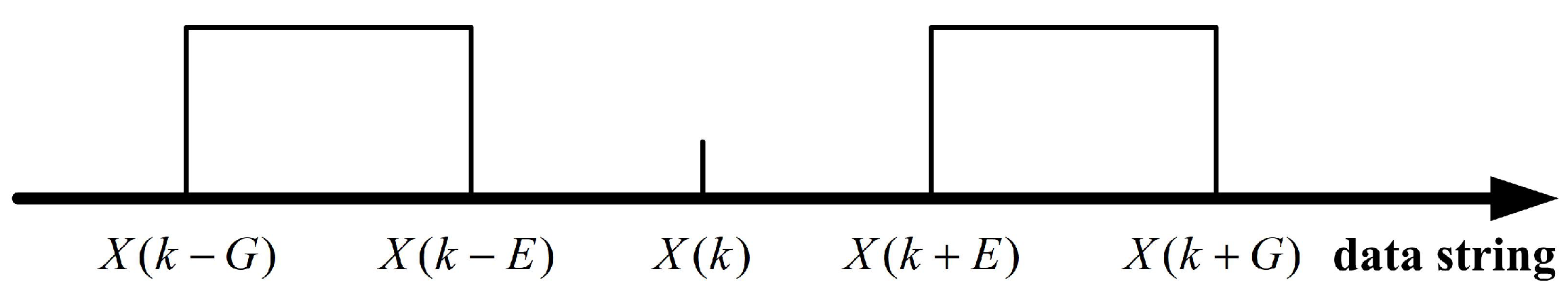
2.1. TPSW Algorithm
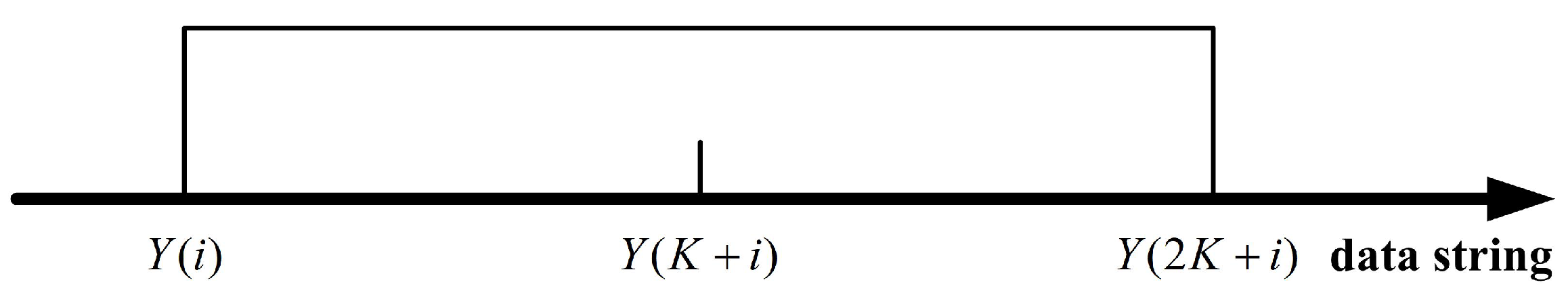
2.2. OTA Algorithm
2.3. Beam Characteristics Scan Algorithm
3. Problem Formulation and Proposed Approach
3.1. Problem Formulation
- Unstable performance due to the experientially set parameters (TPSW and OTA);
- High level environmental and self-noise in low frequency cannot be fully suppressed (beam characteristics scan algorithm).
3.2. Proposed Approach
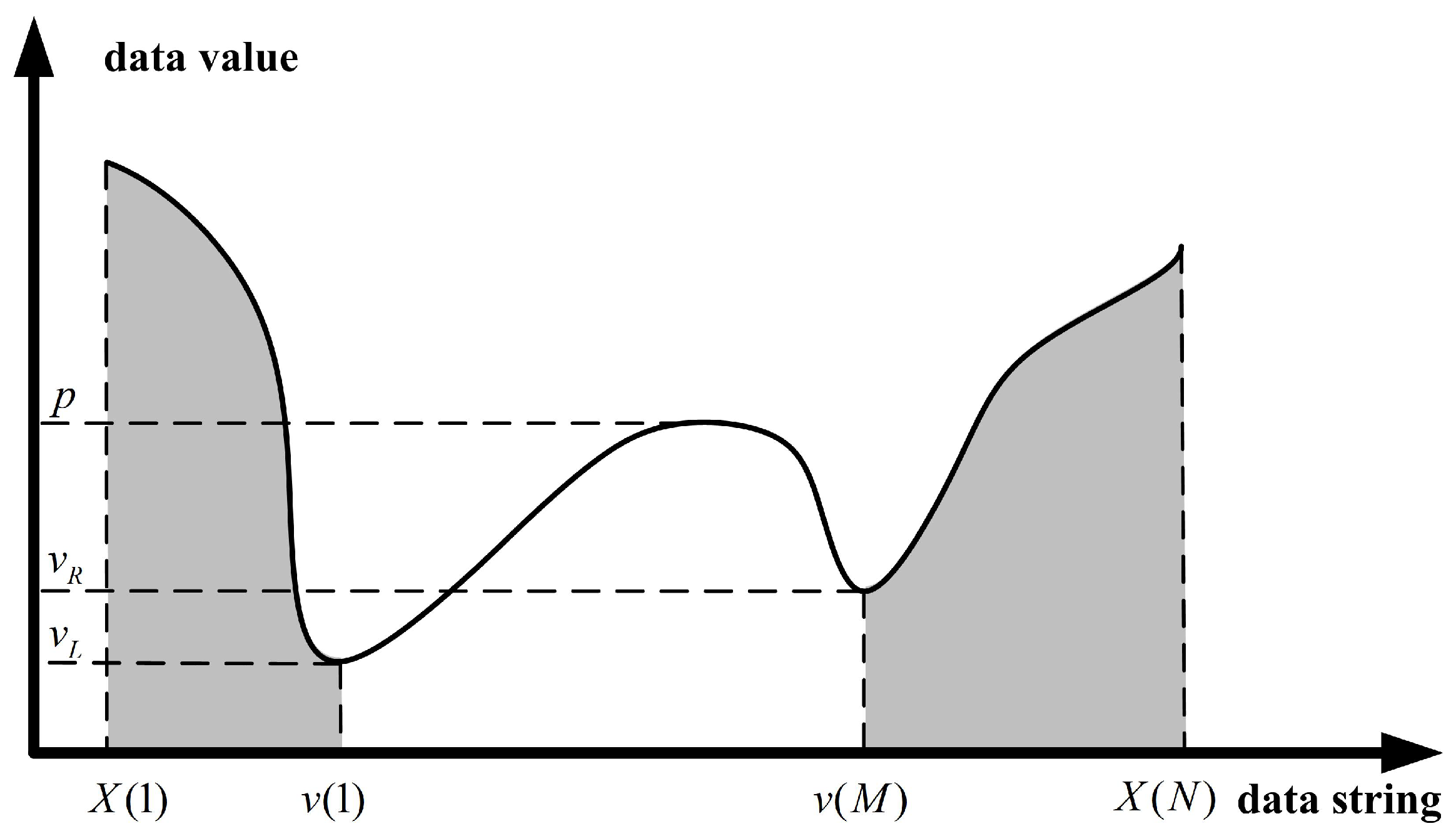
- Step 1. Search all the valley values of data string .
- Step 2. For a given valley , find the third closest left and right peaks as and , and represent the data vector (with the length ) between the two peaks as
- Step 4. Export the normalized data vectorand the whole normalized data string is represented as .
4. Experimental Results and Further Discussion
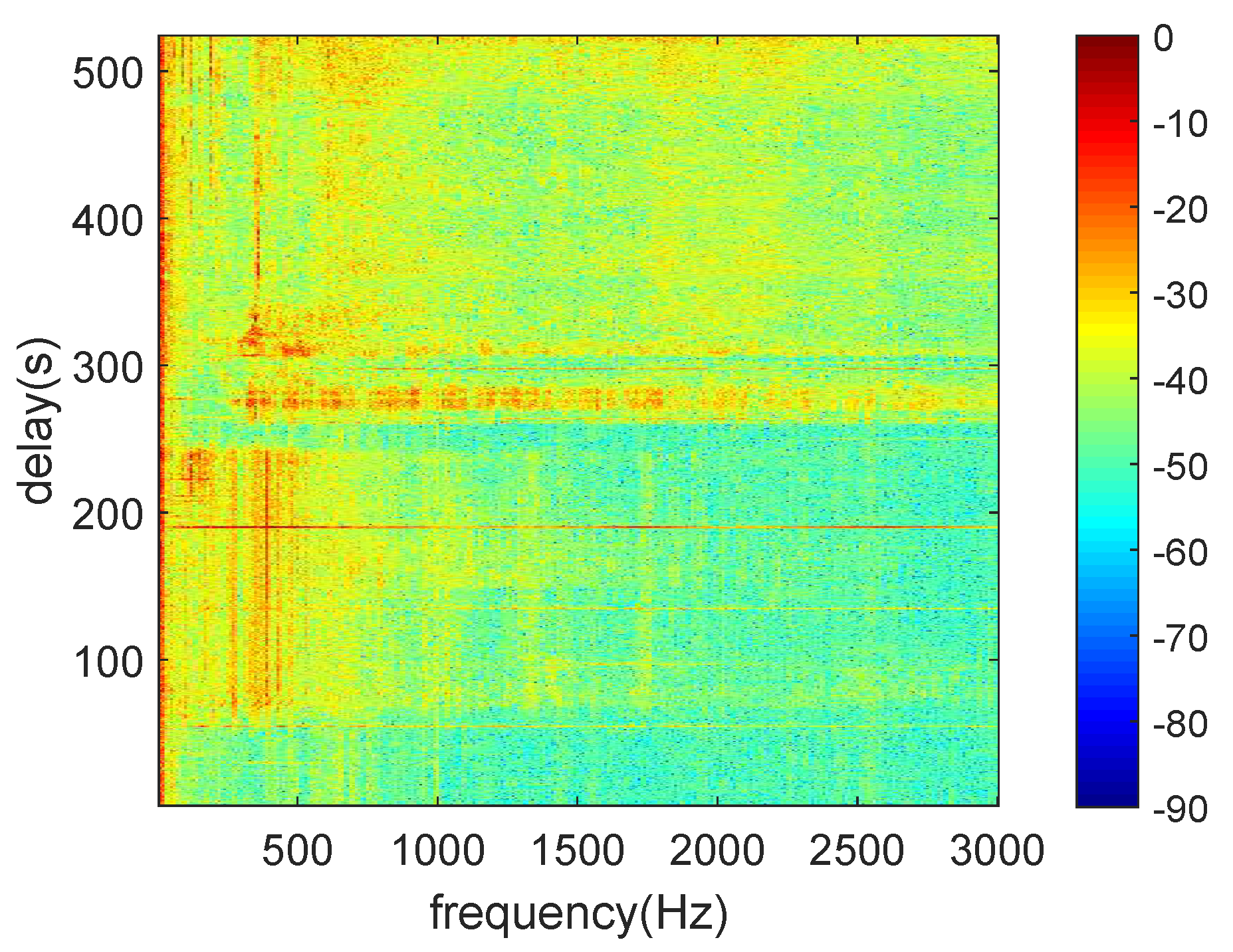
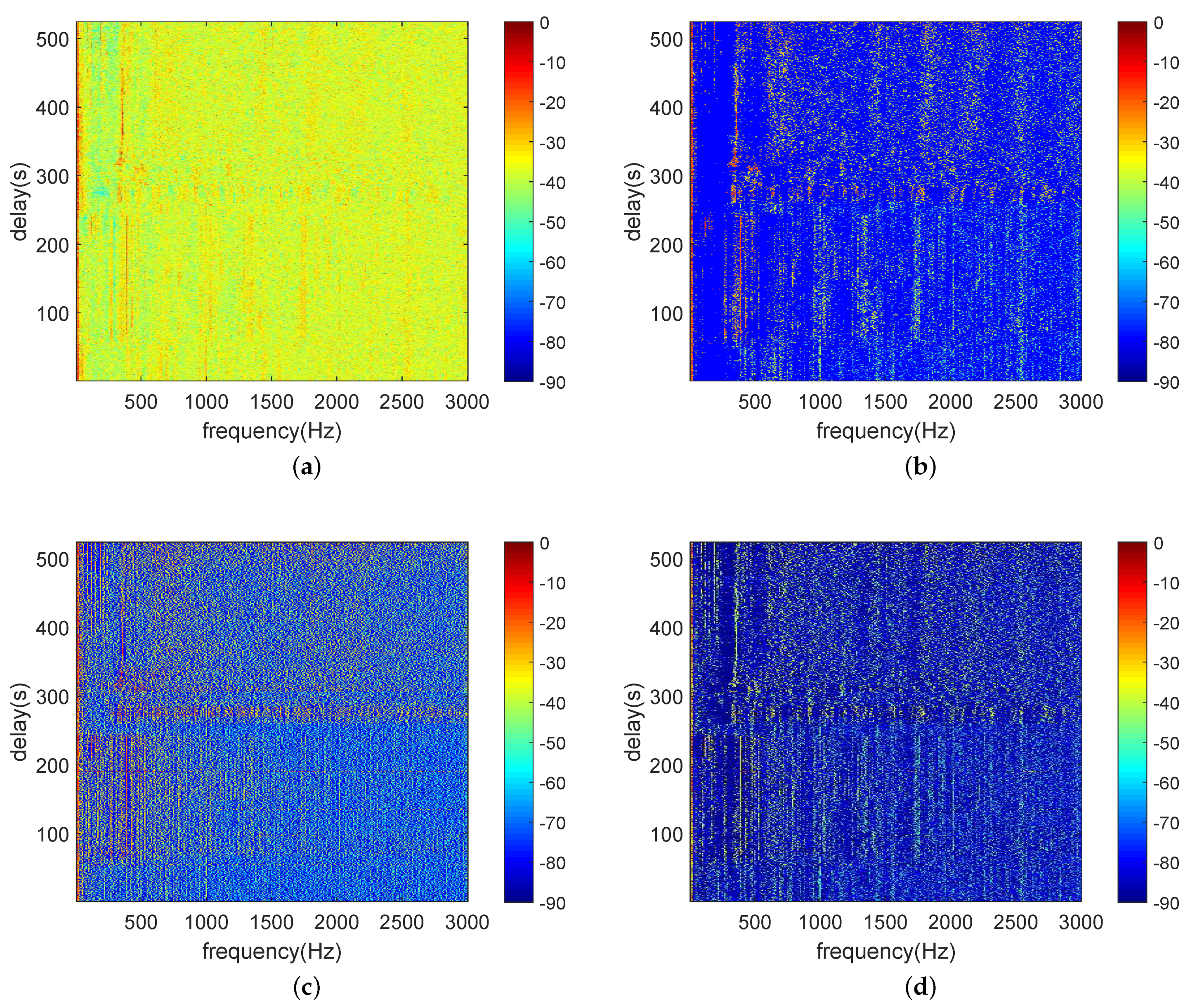
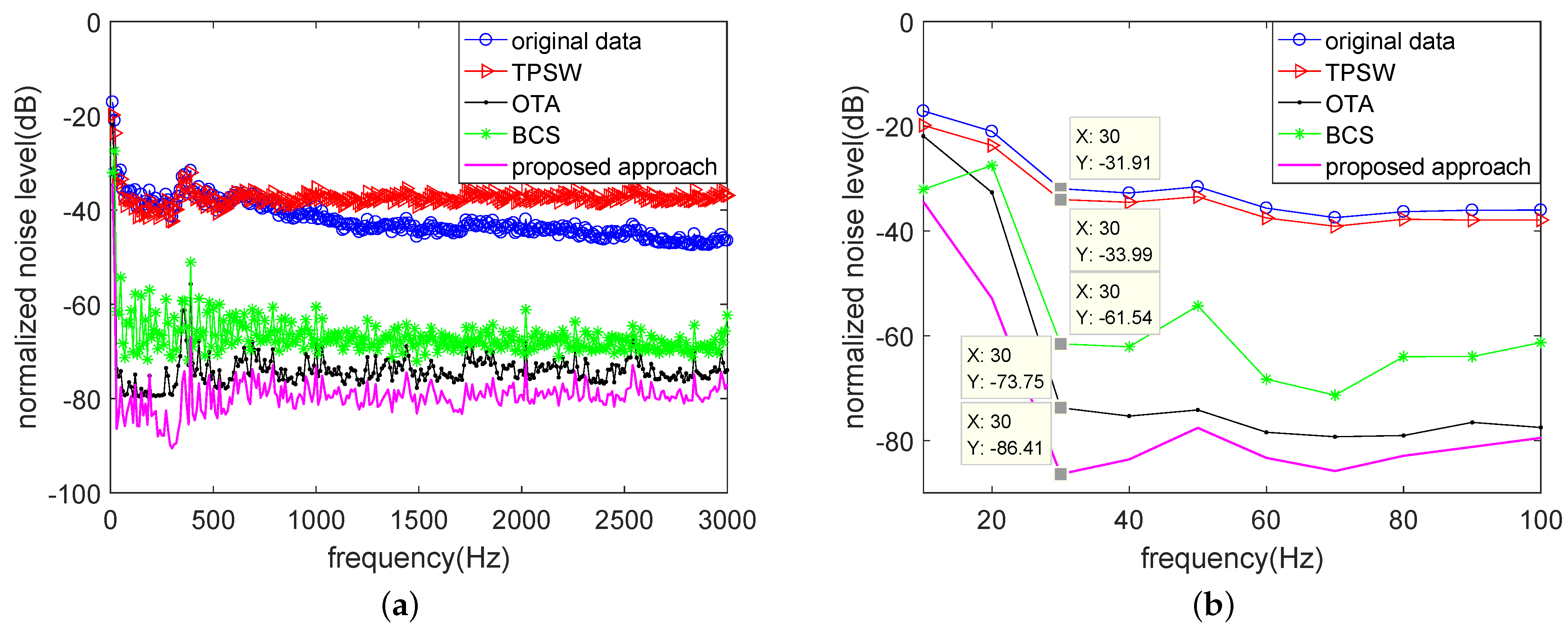
4.1. Analysis of Experimental Results
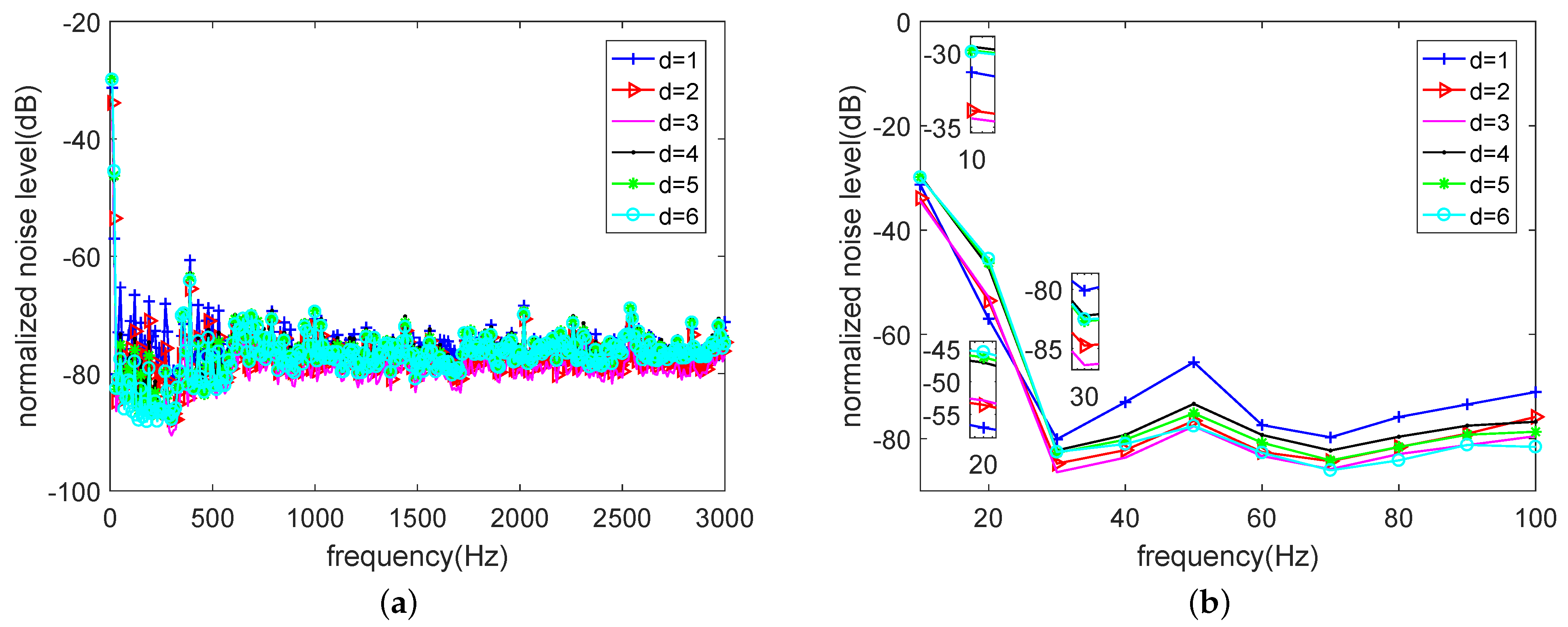
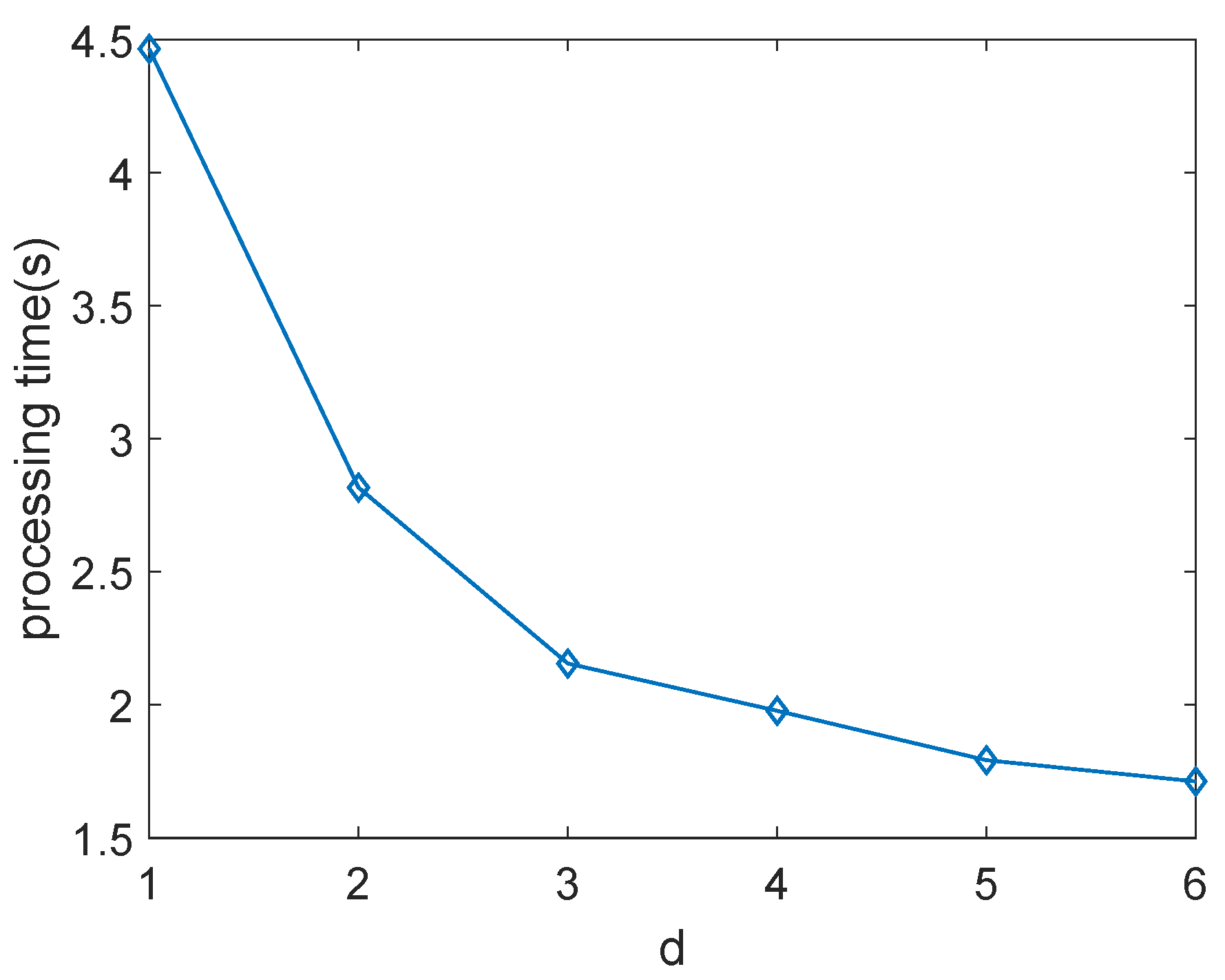
4.2. Further Discussion
5. Conclusions
Author Contributions
Funding
Acknowledgments
Conflicts of Interest
References
- Stergiopoulos, S. Noise normalization technique for beamformed towed array data. J. Acoust. Soc. Am. 1995, 97, 2334–2345. [Google Scholar] [CrossRef]
- Filho, W.S.; de Seixas, J.M.; de Moura, N.N. Preprocessing passive sonar signals for neural classification. IET Radar Sonar Navig. 2011, 5, 605–612. [Google Scholar] [CrossRef]
- Zheng, J. Research on Passive Sonar Display Optimization Technology. Master’s Thesis, Harbin Engineering University, Harbin, China, 2013. (In Chinese). [Google Scholar]
- Struzinski, W.A.; Lowe, E.D. A performance comparison of four noise background normalization schemes proposed for signal detection systems. J. Acoust. Soc. Am. 1984, 76, 1738–1742. [Google Scholar] [CrossRef]
- Li, Q.; Pan, X.; Li, Y. A new algorithm of background equalization in digital sonar. Acta Acust. 2000, 25, 5–9. (In Chinese) [Google Scholar]
- Joo, J.H.; Jun, B.D.; Shin, K.C.; Kim, D.Y. The performance test of the background noise normalization in the narrow band detection. In Proceedings of the UDT Europe, Hamburg, Germany, 27–29 June 2006; pp. 1–4. [Google Scholar]
- Wang, X. Studies on Passive Sonar Broadband Display Method and Bearing Estimation Technology. Master’s Thesis, Northwestern Polytechnical University, Xi’an, China, 2009. (In Chinese). [Google Scholar]
- Kuhn, J.P.; Heath, T.S. Apparatus for and Method of Adaptively Processing Sonar Data. U.S. Patent US5481503A, 2 January 1996. [Google Scholar]
- Bentrem, F.W.; Botts, J.; Summers, J.E. Design of a Signal Normalizer for High-Clutter Active-Sonar Detection. J. Acoust. Soc. Am. 2018, 143, 1760. [Google Scholar] [CrossRef]
- Nielsen, R.O. Sonar Signal Processing; Artech House Publishers: Norwood, MA, USA, 1991. [Google Scholar]
- Qiu, J.; Wang, Y.; Ding, C.; Cheng, Y. Adaptive threshold background normalization algorithm for bearing-time recording. Ship Sci. Technol. 2019, 41, 133–137. (In Chinese) [Google Scholar]
- Struzinski, W.A.; Lowe, E.D. The effect of improper normalization on the performance of an automated energy detector. J. Acoust. Soc. Am. 1985, 78, 936–941. [Google Scholar] [CrossRef]
- Zhu, J.; Wang, X.; Huang, X.; Suvorova, S.; Moran, B. Range sidelobe suppression for using Golay complementary waveforms in multiple moving target detection. Signal Process. 2017, 141, 28–31. [Google Scholar] [CrossRef]


| Algorithms | TPSW | OTA | Beam Characteristics Scan Method | Proposed Approach |
| Time Burden |
Publisher’s Note: MDPI stays neutral with regard to jurisdictional claims in published maps and institutional affiliations. |
© 2021 by the authors. Licensee MDPI, Basel, Switzerland. This article is an open access article distributed under the terms and conditions of the Creative Commons Attribution (CC BY) license (https://creativecommons.org/licenses/by/4.0/).
Share and Cite
Zhu, J.; Peng, C.; Zhang, B.; Jia, W.; Xu, G.; Wu, Y.; Hu, Z.; Zhu, M. An Improved Background Normalization Algorithm for Noise Resilience in Low Frequency. J. Mar. Sci. Eng. 2021, 9, 803. https://doi.org/10.3390/jmse9080803
Zhu J, Peng C, Zhang B, Jia W, Xu G, Wu Y, Hu Z, Zhu M. An Improved Background Normalization Algorithm for Noise Resilience in Low Frequency. Journal of Marine Science and Engineering. 2021; 9(8):803. https://doi.org/10.3390/jmse9080803
Chicago/Turabian StyleZhu, Jiahua, Chengyan Peng, Bingbing Zhang, Wentao Jia, Guojun Xu, Yanqun Wu, Zhengliang Hu, and Min Zhu. 2021. "An Improved Background Normalization Algorithm for Noise Resilience in Low Frequency" Journal of Marine Science and Engineering 9, no. 8: 803. https://doi.org/10.3390/jmse9080803