Identification and Prediction of Ship Maneuvering Motion Based on a Gaussian Process with Uncertainty Propagation

Abstract

Maritime transport plays a vital role in economic development. To establish a vessel scheduling model, accurate ship maneuvering models should be used to optimize the strategy and maximize the economic benefits. The use of nonparametric modeling techniques to identify ship maneuvering systems has attracted considerable attention. The Gaussian process has high precision and strong generalization ability in fitting nonlinear functions and requires less training data, which is suitable for ship dynamic model identification. Compared with other machine learning methods, the most obvious advantage of the Gaussian process is that it can provide the uncertainty of prediction. However, most studies on ship modeling and prediction do not consider the uncertainty propagation in Gaussian processes. In this paper, a moment-matching-based approach is applied to address the problem. The proposed identification scheme for ship maneuvering systems is verified by container ship simulation data and experimental data from the Workshop on Verification and Validation of Ship Maneuvering Simulation Methods (SIMMAN) database. The results indicate that the identified model is accurate and shows good generalization performance. The uncertainty of ship motion prediction is well considered based on the uncertainty propagation technology.

1. Introduction

Maritime transport plays a positive role in promoting the sustainable development of the country’s economy [1], and it is also directly related to environmental pollution [2]. Accurate maritime traffic simulators (MTS) can provide an effective basis for the port and route planning and management [3], and can help liner shipping companies arrange vessel schedule efficiently [4,5]. Moreover, an accurate ship maneuvering model is of great practical value for ship trajectory prediction and controller design [6]. With the rapid development of maritime autonomous surface ships (MASSs) [7], autonomous navigation and collision avoidance systems require a more intelligent digital maneuvering model, which can predict the future dynamics of ships and estimate the uncertainty caused by the actions to be performed.

Modeling techniques for ship dynamic models involve parametric modeling and nonparametric modeling. Parametric modeling must define a complete mathematical structure in advance from a physical viewpoint and subsequently estimate the hydrodynamic derivatives through parameter identification techniques. Classic system identification methods are widely used for hydrodynamic parameter identification, such as least square estimation [8], the recursive prediction error (RPE) method [9]. However, the traditional methods are sensitive to noise, and the multicollinearity will significantly affect the identification accuracy [10]. Over the decades, a great number of new methods have been proposed to solve the above problems. Yoon and Rhee used ridge regression to suppress the parameter drift due to multicollinearity [11]. Revestido Herrero and Velasco Gonzalez proposed a two-step method based on extended Kalman filtering (EKF) to identify the parameters in the nonlinear model [12]. Sutulo and Guedes Soares adopted genetic algorithms (GA) with Hausdorff metric loss function to reduce the influence of white noise on parameter identification [13]. Least squares support vector machine (LS-SVM), with its good robustness and generalization ability, has been applied to various ship parametric model identification, and has been verified by simulation and experiment [14,15]. Recently, Xu et al. proposed an optimal truncated LS-SVM and validated this method by free-running tests [16,17] and planar motion mechanism tests [18]. The main advantage is that it can be successfully used for big data driven modeling or large-scale training set problems. However, parametric models have some inherent limitations. In the specified parametric framework, the unmodeled dynamics caused by external perturbations and noise [19] will greatly impact the parameter estimation. Moreover, the shapes of various unmanned surface vessels (USVs) are irregular, and the traditional parametric models obtained from classic ship types are not completely matched.

Unlike the parametric model, the nonparametric model does not require any predetermined equation framework constructed by prior knowledge [20]. Nonparametric modeling provides a wealth of techniques to extract information from measurement data, which can be translated into knowledge about hydrodynamic systems [21]. The typical representation of nonparametric modeling methods is neural networks. A recursive neural network (RNN) is first used to fit a maneuvering simulation model for surface ships [22]. Zhang and Zou presented the feed-forward neural network with Chebyshev orthogonal basis function for the black-box modeling of ship maneuvering motion [23]. Wang et al. proposed generalized ellipsoidal basis function fuzzy neural networks to identify the motion dynamics of a large tanker [24]. However, NNs require a considerable amount of training data, and the structure of NNs is difficult to determine. Long short-term memory (LSTM) NNs overcome these shortcomings with the transmission of long-term information and have been successfully used to identify USVs [25] and container ships [26]. The kernel-based method requires less training data and has a lower overfitting risk than the NN [27]. Locally weighted learning (LWL) with modified genetic optimization is presented to identify ship maneuvering systems with full-scale trials [28]. $\nu$-SVM is proposed to establish the maneuvering motion model and validated by KVLCC2 ship experimental data [29]. In general, nonparametric modeling alleviates the drawbacks of parametric modeling, i.e., multicollinearity, parameter drifting and unmodeled dynamics.

Recently, the Gaussian process (GP) has drawn attention in nonparametric modeling in marine engineering. GP further strengthens the generalization ability of the kernel method with a priori introduction from a Bayesian perspective. GP is used to identify nonlinear wave forces [30], floating production storage and offloading (FPSO) vessel motion modeling [31], and ship trajectory prediction [32]. Ramire et al. first proposed using a multioutput GP to identify the dynamic model of a container ship [33]. Xue et al. presented a noisy input GP to improve the identification accuracy and verified it by using simulated ship motion data with artificial noise [34]. The experimental data of the KVLCC2 ship were used to construct the GP [35], but the accuracy of prediction in the experiment was not sufficiently high. In the prediction of ship motion based on GP, the prediction output of each time is used as the input to the next iteration, so uncertainty will accumulate. However, this ship dynamic modeling using GP does not consider the propagation of variance.

In this paper, to solve the problem of variance propagation in GP, an approximation method is applied. First, the input is assumed to follow a Gaussian distribution. The predictive distribution is approximated by a moment matching-based technique. To evaluate the effectiveness of the proposed scheme, the simulation case of a container ship and the experimental case of a KVLCC2 ship model from the Hamburg Ship Model Basin (HVSA) are taken as the study object. The identified models are assessed by the prediction error with other motion data not included in the training set.

The remainder of the paper is organized as follows. Section 2 describes the nonparametric ship dynamic model. The algorithms of GP with uncertain input are depicted in Section 3. In Section 4, the identification scheme of the ship and experimental example are presented to demonstrate the applicability of the proposed method. Section 5 summarizes the study with conclusions.

2. Ship Nonparametric Dynamic Model

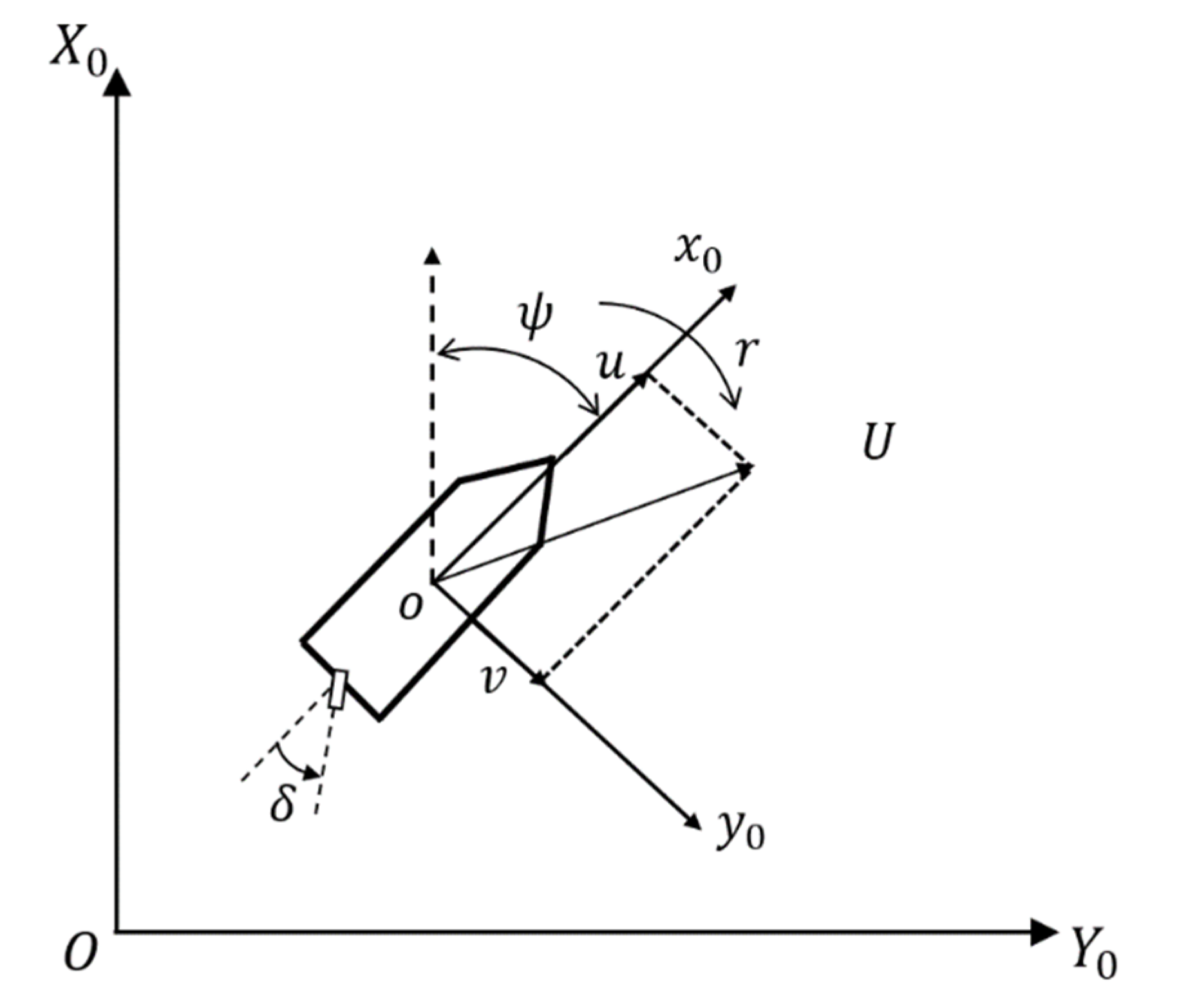
For a surface ship, the dynamic model is usually described by a 3-DOF model, including the motion of surge, sway and yaw. Figure 1 shows the coordinate system of a surface ship maneuvering motion, including the Earth-fixed coordinates $O-X_0{Y}_0$ and body-fixed coordinates $o-x_0{y}_0$. Here, $u,v, \mathrm{and} r$ are the state variables of surge velocity, sway velocity, and yaw rate, respectively, while $\delta$ is the rudder angle and $\psi$ is the heading angle.

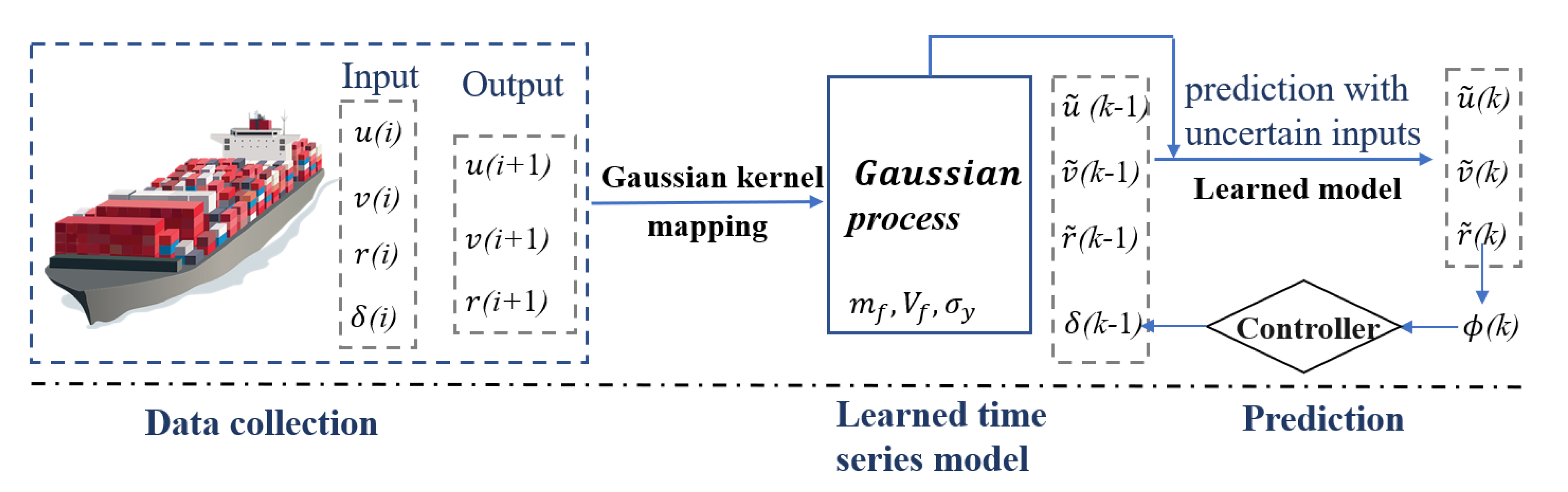
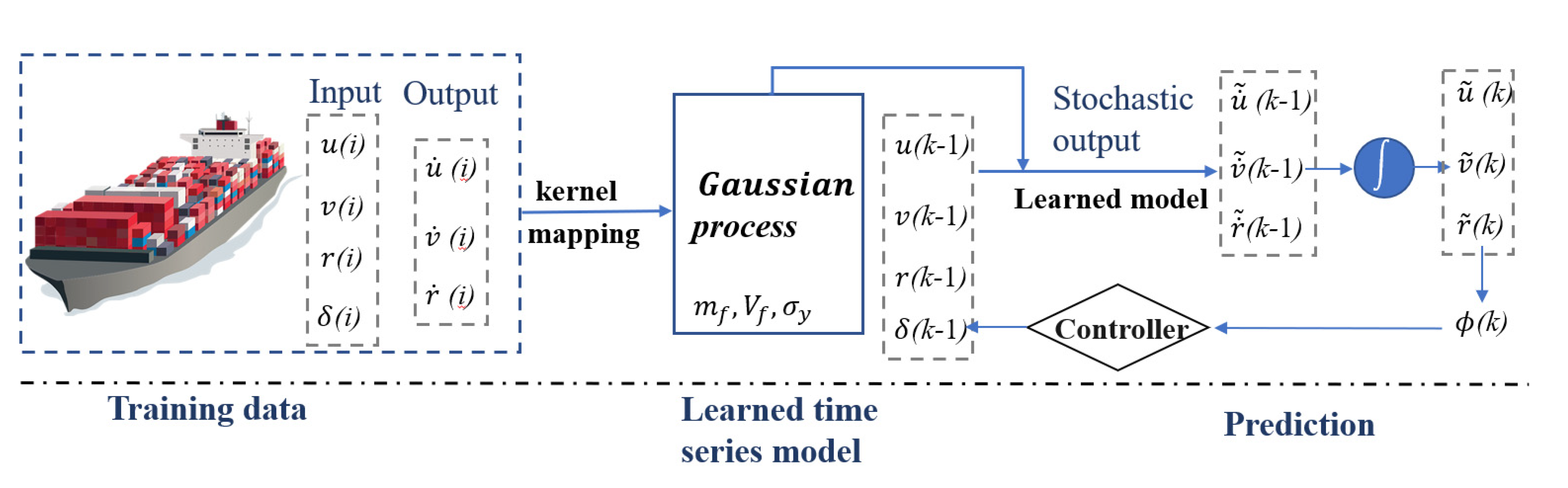
The ship maneuvering system is a nonlinear autoregressive model with an exogenous input (NARX) system [36], and the outputs at the next moment are based on the previous state variables. Figure 2 illustrates the modeling and prediction process of the ship dynamic model. In the first stage, ship motion data are collected by onboard sensors such as IMU and GPS. After data preprocessing, the machine learning technique is used to fit the surrogate time series model. Finally, other motions can be predicted through the learned model. The symbol “~” represents random variables.

According to the relevant studies of nonparametric ship dynamic modeling [25,34], the formulation of the ship discrete nonparametric model is as follows:

$$\begin{array}{c}u\left(k+1\right)=G{P}_1\left(u\left(k\right),v\left(k\right),r\left(k\right),\delta \left(k\right)\right)\\ v\left(k+1\right)=G{P}_2\left(u\left(k\right),v\left(k\right),r\left(k\right),\delta \left(k\right)\right)\\ r\left(k+1\right)=G{P}_3\left(u\left(k\right),v\left(k\right),r\left(k\right),\delta \left(k\right)\right)\end{array}$$

(1)

The selected regressors of the GP are inspired by parametric models, including the Abkowitz [37] and Maneuvering Modeling Group (MMG) models [38]. The ship position variables can be obtained as follows:

$$\begin{array}{c}\dot{x}=ucos\left(\psi \right)-vsin\left(\psi \right)\\ \dot{y}=usin\left(\psi \right)+vcos\left(\psi \right)\end{array}$$

(2)

3. Gaussian Process Regression Framework

3.1. Gaussian Process with Deterministic Input

The following notation with a set of training data is defined:

$$\mathcal{D}=({\left[x_t\right]}_{t=1}^n, {\left[y_t\right]}_{t=1}^N)$$

(3)

where $x_t$ is an input vector, and output $y_t$ is given by

$$\begin{array}{c}y=f\left(x\right)+\omega \\ w~\mathcal{N}\left(0,{\mathsf{\sigma }}_{\omega }{}^2\right)\end{array}$$

(4)

A standard GP is a collection of random variables and can be considered a collection of random variables with a joint Gaussian distribution for any finite subject [39]. GP is specified by the mean function $m\left(x\right)$ and covariance function $k\left(x,x^{\prime }\right)$ as

$$m\left(x\right)=E\left[f\left(x\right)\right]$$

(5)

$$k\left(x,x^{\prime }\right)=E\left[\left(f\left(x\right)-m\left(x\right)\right)\left(f\left(x^{\prime }\right)-m\left(x^{\prime }\right)\right)\right]$$

(6)

where $E$ is the expectation operator. Then, the GP can be written as:

$$f\left(x\right)~GP\left(m\left(x\right),k\left(x,x^{\prime }\right)\right)$$

(7)

The proposed model adopts the commonly used squared exponential covariance function:

$$k\left(x_i,x_j\right)={\mathsf{\sigma }}_f{}^2\exp (-\frac{1}{2}{(x_i-x_j)}^T\mathsf{\Lambda }\left(x_i-x_j\right))$$

(8)

where ${\mathsf{\sigma }}_f$ and $\mathsf{\Lambda }$ are the amplitude and squared length-scale hypermeters, respectively.

Bayesian inference can be defined as the process of fitting a posterior probability model from a prior model with a set of training data $\mathcal{D}$. The GP prior is given as:

$$p(f|X)=\mathcal{N}\left(m\left(X\right),k\left(X,X\right)\right)$$

(9)

With these modeling assumptions in place, the likelihood function can be obtained,

$$p\left(y|f,X\right)={\displaystyle \prod }_{t=1}^n\mathcal{N}\left(y_t;f_t,{\mathsf{\sigma }}_{\omega }{}^2\right)$$

(10)

Then, combining the prior Equation (9) and the likelihood function Equation (10) with the Bayesian rule, the posterior probability distribution and predicted function values $f^{*}$ can be calculated, at a set of deterministic inputs $X^{*}$.

$$\left[\begin{array}{c}{f}^{*}\\ y\end{array}\right]~\mathcal{N}\left(\begin{array}{cc}\left[\begin{array}{c} m\left(X^{*}\right)\\ m\left(X\right)\end{array}\right],& \left[\begin{array}{cc} K\left(X^{*},X^{*}\right)& K\left(X^{*},X\right)\\ K(X,X^{*})& K+{\mathsf{\sigma }}_{\omega }{}^{2}I\end{array}\right]\end{array}\right)$$

(11)

which leads to the RGP regression predictive equations,

𝑝𝑓∗𝑋∗,𝑋,𝑦 =$𝒩$(𝓂,𝓈)

(12)

where the predictive mean and variance function are specified by:

$$m=m\left(X^{*}\right)+K\left(X^{*},X\right){[K\left(X,X\right)+{\mathsf{\sigma }}_{\omega }{}^{2}I]}^{-1}\left(y-m\left(X\right)\right)$$

(13)

$$𝓈=k\left(X^{*},X^{*}\right)-K\left(X^{*},X\right){[K\left(X,X\right)+{\mathsf{\sigma }}_{\omega }{}^{2}I]}^{-1}K\left(X,X^{*}\right)$$

(14)

The hyperparameters in Equation (8) are usually obtained by maximizing the log of the marginal likelihood function. It is defined as [36]:

$$-log p\left(y|X,\theta \right)=\frac{1}{2}{\left(y-m\left(X\right)\right)}^T{\left(K\left(X,X\right)+{\mathsf{\sigma }}_{\omega }{}^{2}I\right)}^{-1}\left(y-m\left(X\right)\right)+\frac{1}{2}log\left|K\left(X,X\right)+{\mathsf{\sigma }}_{\omega }{}^{2}I\right|+\frac{N}{2}log2\pi$$

(15)

This nonlinear and nonconvex optimization problem is usually solved by the gradient ascent-based methods, such as BFGS and the conjugate gradient (CG) algorithm [36].

3.2. Prediction with Uncertain Inputs and Uncertainty Propagation

In Equation (11), we assume that the input is deterministic, while the output is Gaussian distributed. This assumption is true in the one-step prediction. For multiple-step predictions, the traditional method is to recycle the one-step prediction. However, the uncertainties induced by each successive prediction cannot be ignored in the time-series tasks [40].

The uncertainty propagation problem can be addressed assuming that the input follows a Gaussian distribution [41]:

$$\widetilde{X^{*}}~\mathcal{N}\left(\widetilde{\mu ,}\tilde{\sum }\right)$$

(16)

For convenience of expression and marking, the input variables are divided into speed variable $x$ and control variable $𝓊$, as $X^{*}=\left[x,𝓊\right]$. The mean and variance are given as:

$$\begin{array}{c}\tilde{\mu }={[ \mu ,E\left[𝓊\right] ]}^T\\ {\displaystyle \tilde{\sum }}=\left[\begin{array}{cc}\sum & Cov\left[x,𝓊\right]\\ Cov\left[𝓊,x\right]& Var\left[𝓊\right]\end{array}\right]\end{array}$$

(17)

where $E\left[𝓊\right]$ and $Var\left[𝓊\right]$ are the mean and variance of the control variable; $Cov\left[x,𝓊\right]=E\left[x𝓊\right]-\mu E\left[𝓊\right]$.

The predictive distribution can be obtained by integrating over the input:

$$p(X^{*}|\widetilde{\mu ,}\tilde{\sum })=\int p(f(\widetilde{X^{*}})|\widetilde{X^{*}})p(\widetilde{X^{*}}|\widetilde{\mu ,}\tilde{\sum })d\widetilde{X^{*}}$$

(18)

However, this integration cannot be analytically computed, since the Gaussian distribution is mapped through a nonlinear function. Taylor approximation [40] or moment matching [42] is commonly used to approximate the integration. The computation of the Taylor approximation is expensive because it accounts for the gradient of the posterior mean and variance of the input. In this paper, moment matching is chosen. The moment matching method assumes that the unknown distribution only has two parameters: the mean and the variance. The mean and variance at an uncertain input can be computed by the laws of iterated expectations and conditional variances [42]:

$$m\left(\widetilde{X^{*}}\right)=E_{\widetilde{X^{*}}}\left[E\right[X^{*}]]$$

(19)

$${\sigma }^2\left(\widetilde{X^{*}}\right)=E_{\widetilde{X^{*}}}\left[Var\left[X^{*}\right]\right]+Va{r}_{\widetilde{X^{*}}}\left[E\right[X^{*}]]$$

(20)

Then, the predicted mean and variance at time t + 1 are given as:

$${\mu }_{t+1}={\mu }_t+m\left(\widetilde{X^{*}}\right)$$

(21)

$${\sum }_{t+1}={\sum }_t+Cov\left[x_t,y_t\right]+Cov\left[y_t,x_t\right]$$

(22)

4. Case Study

4.1. Simulation Study on a Container Ship

The first case uses the simulation maneuvers of a large container ship. The selected parametric numerical model is a nonlinear 4-degree-of-freedom (DOF) dynamic model [43]. The main particulars of the container ship are listed in

Table 1. Particulars of the container ship.

Elements	Values
Length (L)	175$\mathrm{m}$
Breadth	25.4 m
Displacement ($\nabla$)	21,222${ \mathrm{m}}^3$
Aspect ratio	1.8219
Mean draft	8.5 m
Transverse metacenter	10.39 m
Height from keel to center of buoyancy	4.6145 m
Rudder area	33.0376${ \mathrm{m}}^2$
Rudder speed ($\dot{\delta }$)	2.5 deg/s

. The model has been verified by experiments, which can well reflect the complex dynamic characteristics of the container ship. It is widely used in the testing of system identification algorithms [33,44].

The parametric maneuvering model is given as follows [43]:

$$\begin{array}{c}\left(m-X_{\dot{u}}^{ }\right)\dot{u}-\left(m-Y_{\dot{v}}^{ }\right)vr = F_X\\ \left(m-Y_{\dot{v}}^{ }\right)\dot{v}+\left(m-X_{\dot{u}}^{ }\right)ur-Y_{\dot{r}}^{ }\dot{r}=F_Y\\ \left(I_x-K_{\dot{p}}^{ }\right)\dot{p}=F_K-WGM\phi \\ \left(I_z-N_{\dot{r}}^{ }\right)\dot{r}+N_{\dot{v}}^{ }\dot{v}=F_N\end{array}$$

(23)

where $m$ denotes the ship mass, $W$ is the weight of the displaced water, $GM$ is the metacenter height.$I_x$ and $I_z$ denote the moments of inertia of the ship about the ${\mathrm{x}}_0$, ${\mathrm{z}}_0$ axes. $X_{\dot{u}}^{ }$, $Y_{\dot{v}}^{ }$, $Y_{\dot{r}}^{ }$, $N_{\dot{v}}^{ },$ and $N_{\dot{r}}^{ }$ are acceleration derivatives which can be determined using potential theory. $F_X$ $F_Y$ $F_K,$ and $F_N$ are the forces and moment disturbing quantity at ${\mathrm{x}}_0$-axis,${ \mathrm{y}}_0$-axis, and ${\mathrm{z}}_0$-axis, respectively. The nonlinear forces and moments are composed of Taylor expansion of hydrodynamic coefficient and speed.

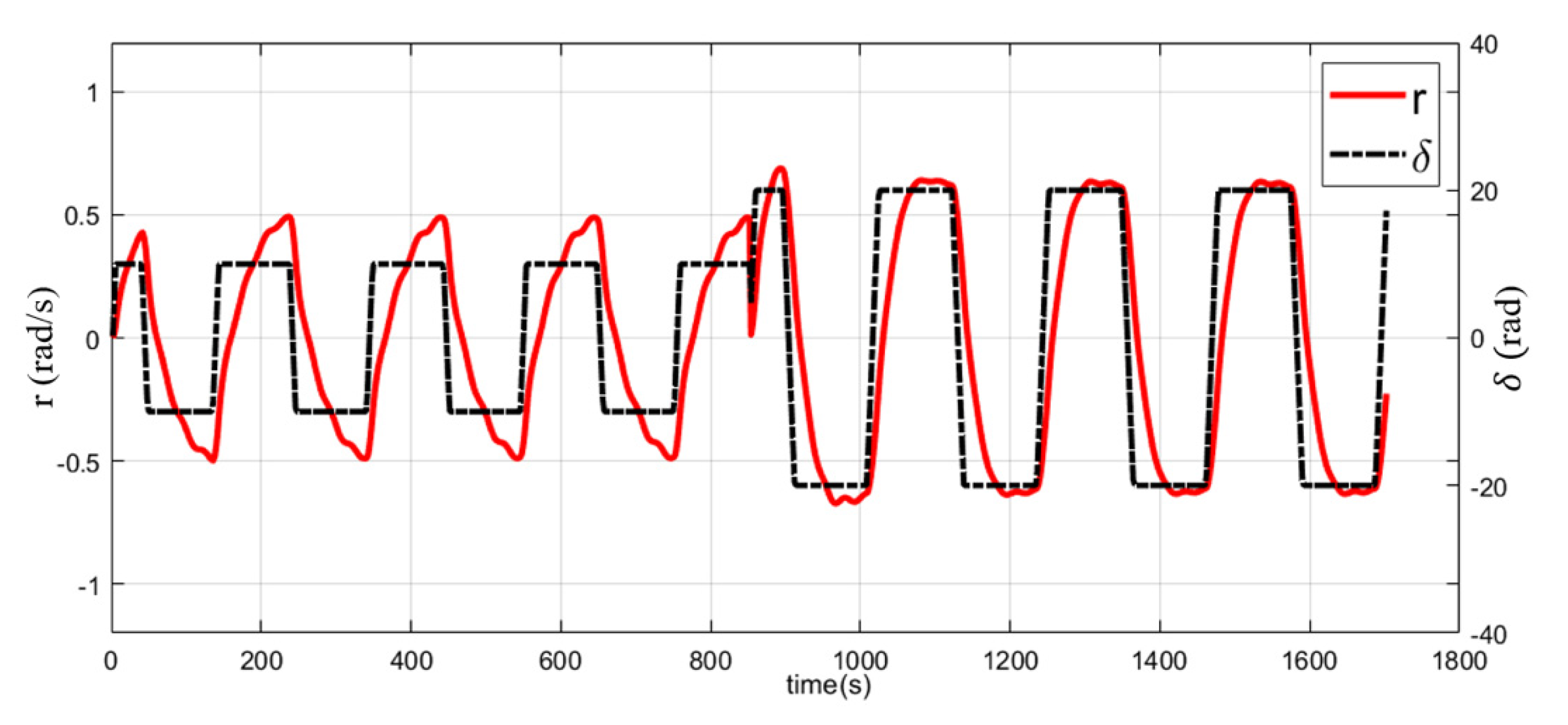
With the 4-DOF model, 2 groups of maneuvers, including 10$°$/10$°$ and 20$°$/20$°$ zigzag tests, are undertaken under the following initial conditions: $u_0=7 \mathrm{m}/\mathrm{s}$, $v_0=0 \mathrm{m}/\mathrm{s}$, $r_0=7 \mathrm{m}/\mathrm{s}$, ${\delta }_0=0 \mathrm{rad}$ and the propeller velocity is fixed at $70 \mathrm{rpm}$. Each maneuver lasted for 850 s, and the simulation interval was 0.1 s. The timeseries of the yaw velocity and rudder angle are shown in Figure 3.

With 2 s as the time interval of the training data, 850 points of the above training data are used to train the GP hyperparameters with maximum likelihood. All calculations are performed in MATLAB R2020a with 4.0 GHz CPU and 16 GB RAM. PILCO toolbox [45] with BFGS and CG algorithms is used to train the Gaussian process. The training process took 9 s in total and trained 3 GPs in Equation (1). The optimization parameter settings of each GP are listed in

Table 2. Selection of the GP parameters for the container ship.

	$\mathit{G}{\mathit{P}}_1$	$\mathit{G}{\mathit{P}}_2$	$\mathit{G}{\mathit{P}}_3$
$\mathsf{\Lambda }$	[12.65, 19.68, 0.27, 8.50${]}_{diag}$	[15.96, 3.53, 0.15, 14.15${]}_{diag}$	[41.18, 3.44, 0.02, 1.90${]}_{diag}$
${\mathsf{\sigma }}_f$	5.2593	1.4911	0.0117
${\mathsf{\sigma }}_{\omega }$	0.0158	0.0231	2.96 × 10−4

.

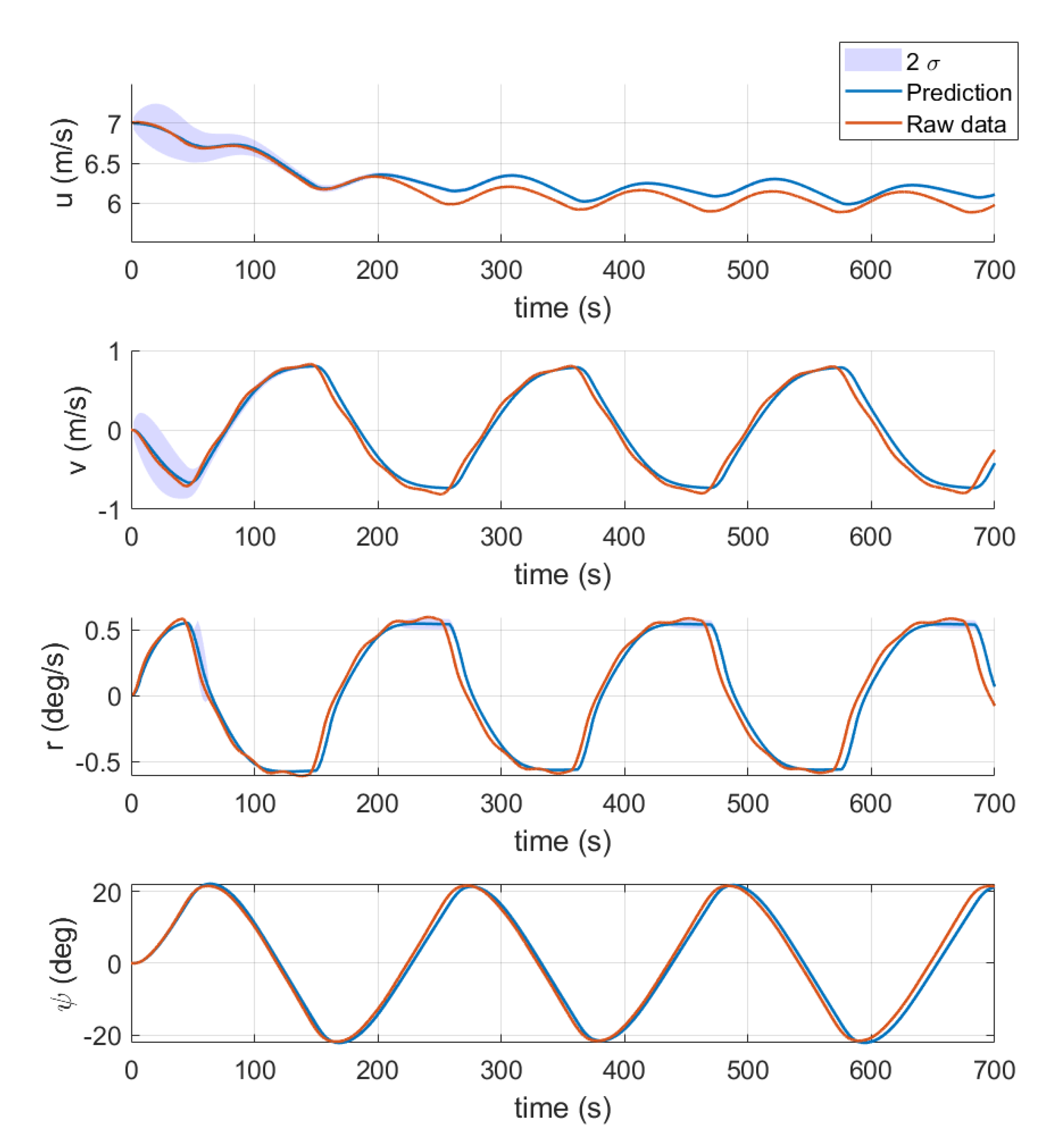
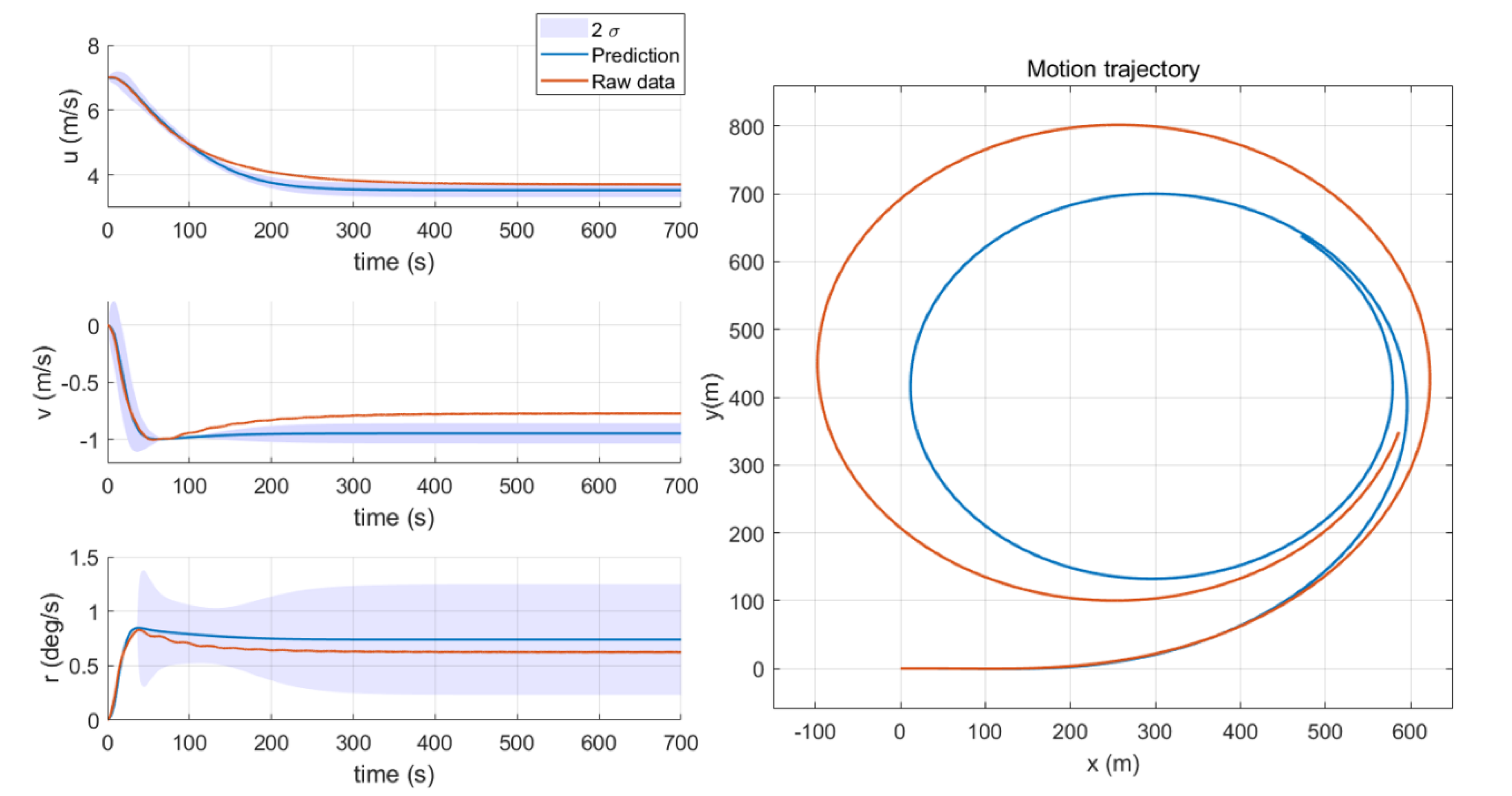
Generalization verification is necessary for system identification. The ability of the identified model to predict other motions not included in the training data is called generalization. The generalization performance of the trained model is verified by predicting the motions, including the 15$°$/15$°$ zigzag maneuver and port 30$°$ turning circle test. The prediction results of the 15$°$/15$°$ zigzag test are shown in Figure 4, where the predictions are compared with the raw data. The prediction results are consistent with the raw data. The prediction variance is also plotted in the figure and shows that the uncertainty is small. The prediction results of the 30$°$ turning circle test are shown in Figure 5. The prediction results can well track the tendency of the raw data. The uncertainty in Figure 5 is much higher than that in Figure 4 because the training data, including 10$°$/10$°$ and 20$°$/20$°$ zigzag tests, completely reflect the dynamic characteristics of the ship when the rudder angle is less than 20$°$. However, the dynamic characteristics of a rudder angle of 30$°$ are not included in the information range provided by the training data. Under this condition, the identified model can predict the motion of a large rudder angle with good generalization ability and maintains good accuracy while providing high uncertainty of prediction through the proposed method.

The root mean square error (RMSE) is applied to evaluate the model performance and is defined as:

$$RMSE=\sqrt{\frac{1}{n}{\displaystyle \sum }_{i=1}^n{(\widehat{y_i}-y_i)}^2}$$

(24)

where $\widehat{y_i}$ is the prediction result, and $y_i$ is the raw value. The RMSEs of the 15$°$/15$°$ zigzag maneuver are listed in

Table 3. Prediction accuracy assessed by the RMSE of the 15°/15° zigzag text.

	RMSE
Surge speed	0.1130
Sway speed	0.0816
Yaw rate	0.0806

with each DOF.

4.2. Experimental Study of a Ship Scale Model

The experimental dataset of KCLCC2 from SIMMAN is used to further validate the proposed method. KVLCC2 is a scale model of large tankers. The main particulars of the scale ship model are detailed in

Table 4. Particulars of KVLCC2.

Elements	Values
$L_{pp}$ (m)	7.0
$B$ (m)	1.1688
$D$ ($\mathrm{m}$)	0.6563
Displacement (${\mathrm{m}}^3$)	3.2724
Draught (m)	0.4550
Beam coefficient	0.8098
Nominal speed (m/s)	1.18
Rudder speed ($\dot{\delta }$)	15.8 deg/s

. The model free-running tests are performed by the Hamburg Ship Model Basin (HVSA).

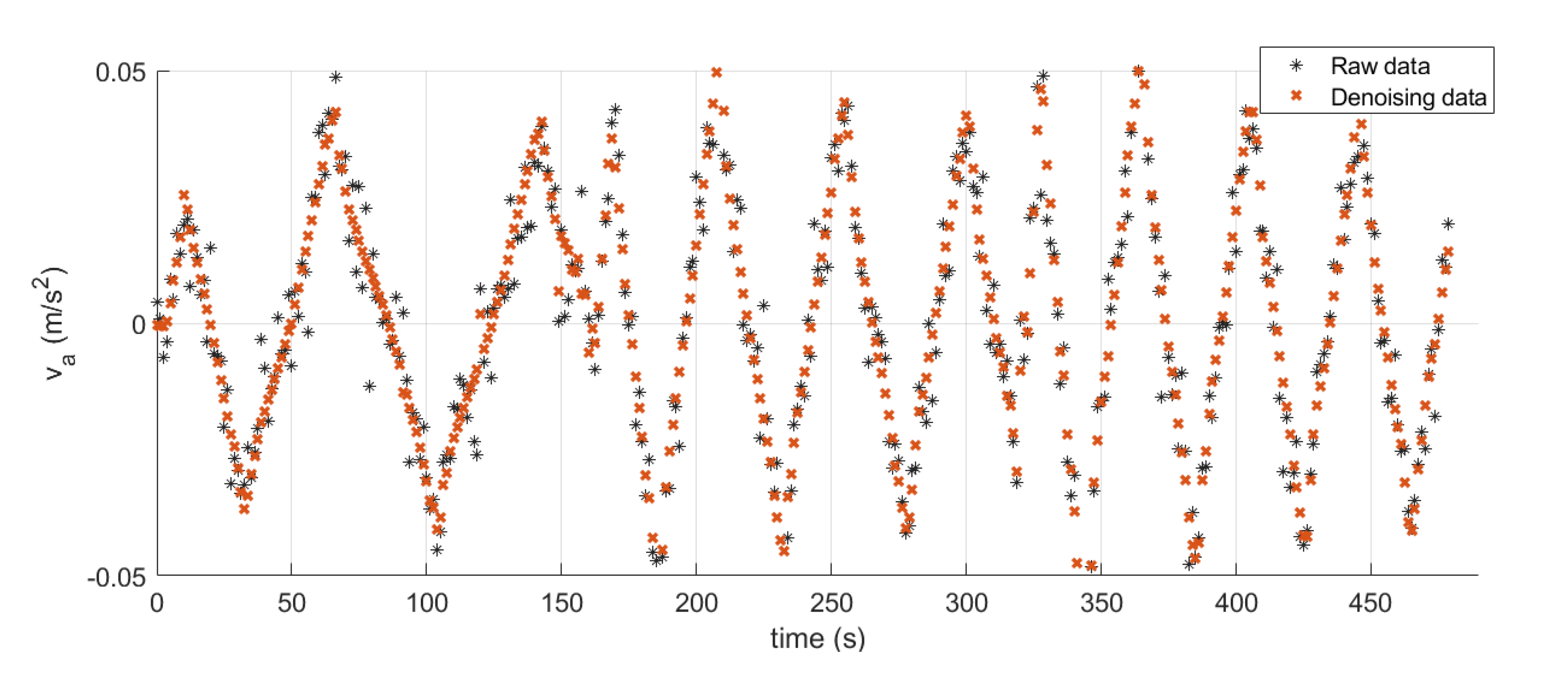
There is some interference and noise in the experimental dataset. Directly taking the speed as the input and output will reduce the identification accuracy. Using the acceleration obtained by the speed difference as the prediction output can effectively alleviate the influence of noise [29], and the new flowchart is shown in Figure 6.

To include more dynamic characteristic information of the ship, the experimental data of 10$°$/5$°$, 20$°$/5$°$ and 30$°$/5$°$ zigzag maneuvers are used to train the GP. Moreover, the empirical Bayes method [46] is applied here to reduce the noise of acceleration with ‘wdenoise’ MATLAB function. More details of the empirical Bayes denoising method for ship motion data can be found in our previous study [47]. Figure 7 shows the effect of noise reduction. There are 800 training points with a time interval of 0.6 s. It took 10.1 s to train 3 GPs for the ship maneuvering system, and the obtained hyperparameter settings are shown in

Table 5. Selection of the GP parameters for the container ship.

	$\mathit{G}{\mathit{P}}_{\mathbf{1}}$	$\mathit{G}{\mathit{P}}_{\mathbf{2}}$	$\mathit{G}{\mathit{P}}_{\mathbf{3}}$
$\mathsf{\Lambda }$	[10.75, 0.04, 0.75, 1.04${]}_{diag}$	[0.52, 1.68, 0.07, 1.35${]}_{diag}$	[0.24, 0.15, 0.03, 0.56${]}_{diag}$
${\mathsf{\sigma }}_f$	0.0277	0.0430	0.0059
${\mathsf{\sigma }}_{\omega }$	0.0050	0.0017	2.16 × 10−4

.

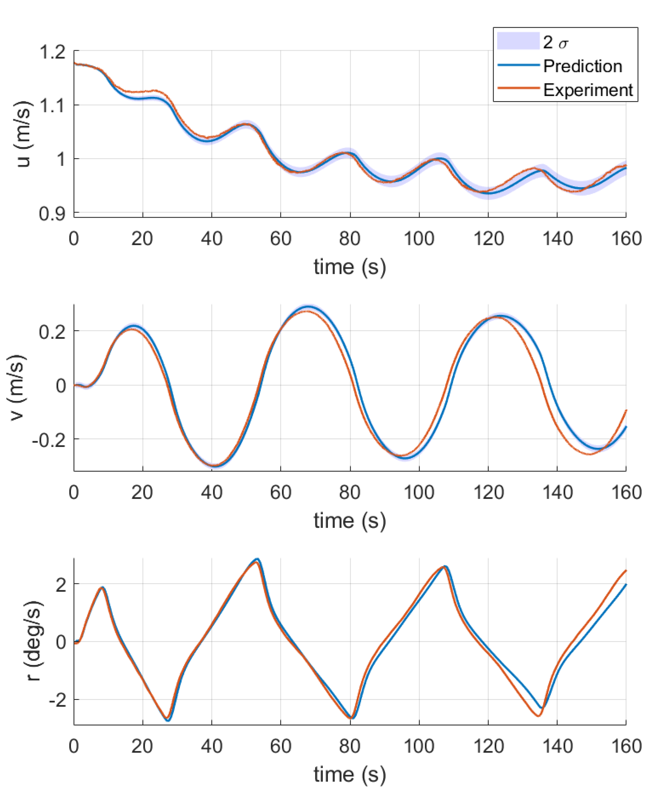
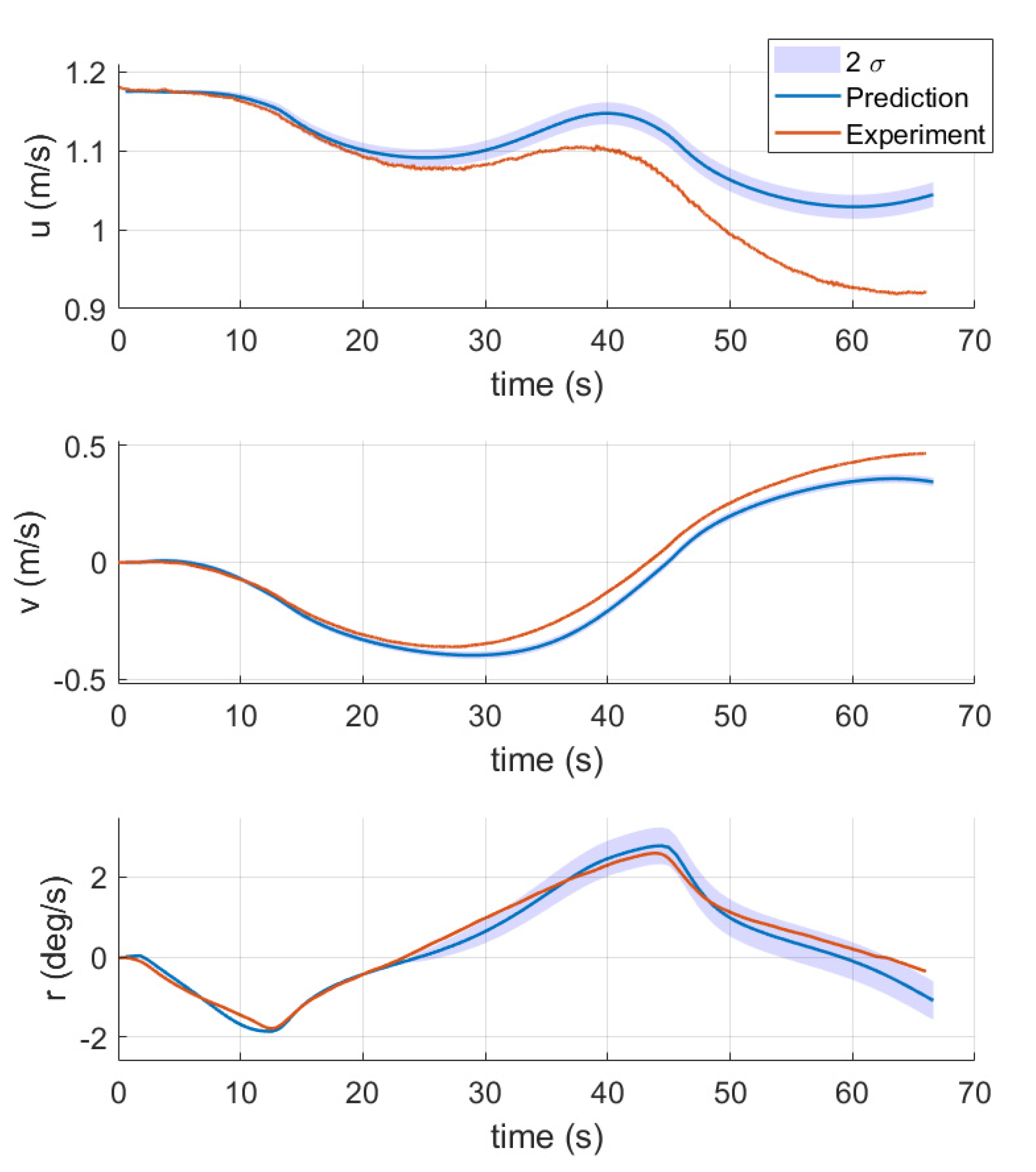
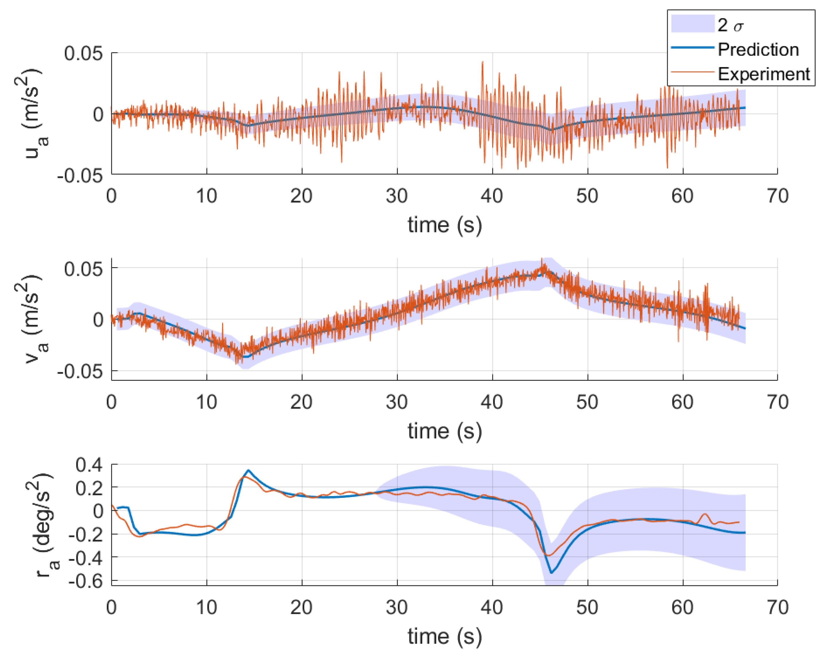
Then, the identified model is validated by comparing the experimental data with predictions of 15$°$/5$°$, 35$°$/5$°$ and 10$°$/10$°$ zigzag maneuvers, as shown in Figure 8, Figure 9 and Figure 10. The accuracy of the prediction speed assessed by RMSE is listed in

Table 6. Prediction accuracy assessed by the RMSE of KVLCC2 with the proposed method.

-	$\mathbf{15}\mathbf{°}$$\mathbf{/}\mathbf{5}\mathbf{°}$	$\mathbf{35}\mathbf{°}$$\mathbf{/}\mathbf{5}\mathbf{°}$	$\mathbf{10}\mathbf{°}$$\mathbf{/}\mathbf{10}\mathbf{°}$
Surge speed	0.0070	0.0240	0.0539
Sway speed	0.0248	0.0541	0.0511
Yaw rate	0.0028	0.0099	0.0044

. In the similar study [29], the same three sets of training data were used for training the nu-SVM. The prediction error of the proposed method can be compared with the nu-SVM in [29]. Figure 8 and Figure 9 show that the experimental data and prediction follow similar trends, and the cumulative deviation is small. The comparison results between Table 6 and the error results in [29] indicate that the proposed method has stronger prediction ability than nu-SVM. However, in Figure 10, the deviation between prediction speed and experiment is obvious, especially in surge motion. The predicted acceleration is also plotted in Figure 11 to analyze the reason. There is a strong oscillation in the measurements of the surge speed. This oscillation in accretion causes a cumulative deviation in speed. As for the uncertainty, it can be observed that the variance of the predictions of the experiment is bigger than the simulation in the previous case. This is because there are more disturbances and noises in the experiment than the simulation.

5. Discussion and Conclusions

In this work, a novel identification modeling and prediction scheme based on GP is proposed to identify the ship nonparametric maneuvering model. By introducing the moment matching approximation method, the multi-step prediction uncertainty of ship motion can be propagated. The performance of the proposed method has been tested with a large container ship and a scale ship model and shows good accuracy and generalization ability. Moreover, the uncertainty of propagation can help drivers or controllers make safe decisions. Through the simulation of the container ship, it is proven that the prediction uncertainty obtained by the proposed method is reliable enough. Where there is less dynamic information in the training data, the prediction uncertainty of turning circle motion is larger than that of zigzag maneuver. In addition, it has been demonstrated that the performance of the presented approach is superior to the nu-SVM method in the experimental case. There are also some limitations of this study: (1) The proposed method needs to spend more calculation time due to consider the uncertainty propagation compared with other methods. The sparse method can be used to improve computational efficiency. (2) Both the two verified cases in this paper are container ships. The applicability of the model to other ship types, especially new unmanned ships, needs further study.

Future work includes two main tasks: (1) Although the presented method has been verified by simulation and experimental data, full-scale trials with disturbances should be performed, including waves, currents, and wind. In this environment, the uncertainty prediction provided by this method will have great application value. (2) This method can be used in modern controllers such as model predictive control. The uncertainty of predictions can be introduced in the cost function to construct a cautious controller.

References

- Akbulaev, N.; Bayramli, G. Maritime transport and economic growth: Interconnection and influence (an example of the countriesin the Caspian sea coast; Russia, Azerbaijan, Turkmenistan, Kazakhstan and Iran). Mar. Policy 2020, 118. [Google Scholar] [CrossRef]
- Bagoulla, C.; Guillotreau, P. Maritime transport in the French economy and its impact on air pollution: An input-output analysis. Mar. Policy 2020, 116. [Google Scholar] [CrossRef]
- Dui, H.; Zheng, X.; Wu, S. Resilience analysis of maritime transportation systems based on importance measures. Reliab. Eng. Syst. Saf. 2021, 209. [Google Scholar] [CrossRef]
- Dulebenets, M.A. A comprehensive multi-objective optimization model for the vessel scheduling problem in liner shipping. Int. J. Prod. Econ. 2018, 196, 293–318. [Google Scholar] [CrossRef]
- Pasha, J.; Dulebenets, M.A.; Fathollahi-Fard, A.M.; Tian, G.; Lau, Y.; Singh, P.; Liang, B. An integrated optimization method for tactical-level planning in liner shipping with heterogeneous ship fleet and environmental considerations. Adv. Eng. Inform. 2021, 48. [Google Scholar] [CrossRef]
- Fossen, T.I. Handbook of Marine Craft Hydrodynamics and Motion Control; John Wiley & Sons, Ltd.; John Wiley & Sons, Ltd.: Chichester, UK, 2011. [Google Scholar]
- Liu, Z.; Zhang, Y.; Yu, X.; Yuan, C. Unmanned surface vehicles: An overview of developments and challenges. Annu. Rev. Control 2016, 41, 71–93. [Google Scholar] [CrossRef]
- Abkowitz, A.M. Measurement of Hydrodynamic Characteristics from Ship Maneuvering Trials by System Identification. 1980. Available online: https://trid.trb.org/view/157366 (accessed on 24 July 2021).
- Zhou, W.-W.; Blanke, M. Identification of a class of nonlinear state-space models using RPE techniques. In Proceedings of the 1986 25th IEEE Conference on Decision and Control, Athens, Greece, 10–12 December 1986; pp. 1637–16410. [Google Scholar]
- Luo, W.; Li, X. Measures to diminish the parameter drift in the modeling of ship manoeuvring using system identification. Appl. Ocean Res. 2017, 67, 9–20. [Google Scholar] [CrossRef]
- Yoon, H.K.; Rhee, K.P. Identification of hydrodynamic coefficients in ship maneuvering equations of motion by Estimation-Before-Modeling technique. Ocean Eng. 2003, 30, 2379–2404. [Google Scholar] [CrossRef]
- Araki, M.; Sadat-Hosseini, H.; Sanada, Y.; Tanimoto, K.; Umeda, N.; Stern, F. Estimating maneuvering coefficients using system identification methods with experimental, system-based, and CFD free-running trial data. Ocean Eng. 2012, 51, 63–84. [Google Scholar] [CrossRef] [Green Version]
- Sutulo, S.; Guedes Soares, C. An algorithm for offline identification of ship manoeuvring mathematical models from free-running tests. Ocean Eng. 2014, 79, 10–25. [Google Scholar] [CrossRef]
- Zhu, M.; Sun, W.; Hahn, A.; Wen, Y.; Xiao, C.; Tao, W. Adaptive modeling of maritime autonomous surface ships with uncertainty using a weighted LS-SVR robust to outliers. Ocean Eng. 2020, 200. [Google Scholar] [CrossRef]
- Wang, Z.; Zou, Z.; Guedes Soares, C. Identification of ship manoeuvring motion based on nu-support vector machine. Ocean Eng. 2019, 183, 270–281. [Google Scholar] [CrossRef]
- Xu, H.; Soares, C.G. Hydrodynamic coefficient estimation for ship manoeuvring in shallow water using an optimal truncated LS-SVM. Ocean Eng. 2019, 191. [Google Scholar] [CrossRef]
- Xu, H.; Hinostroza, M.A.; Wang, Z.; Guedes Soares, C. Experimental investigation of shallow water effect on vessel steering model using system identification method. Ocean Eng. 2020, 199. [Google Scholar] [CrossRef]
- Xu, H.; Hassani, V.; Guedes Soares, C. Uncertainty analysis of the hydrodynamic coefficients estimation of a nonlinear manoeuvring model based on planar motion mechanism tests. Ocean Eng. 2019, 173, 450–459. [Google Scholar] [CrossRef]
- Haranen, M.; Pakkanen, P.; Kariranta, R.; Salo, J. White, grey and black-box modelling in ship performance evaluation. In Proceedings of the 1st Hull performence & insight conference (HullPIC), Castello di Pavone, Italy, 13–15 April 2016; pp. 115–127. [Google Scholar]
- Ljung, L. Black-box models from input-output measurements. In Proceedings of the 18th IEEE Instrumentation and Measurement Technology Conference, Budapest, Hungary, 21–23 May 2001. [Google Scholar]
- Brunton, S.L.; Noack, B.R.; Koumoutsakos, P. Machine learning for fluid mechanics. Annu. Rev. Fluid Mech. 2020, 52, 477–508. [Google Scholar] [CrossRef] [Green Version]
- Moreira, L.; Guedes Soares, C. Dynamic model of manoeuvrability using recursive neural networks. Ocean Eng. 2003, 30, 1669–1697. [Google Scholar] [CrossRef]
- Zhang, X.-G.; Zou, Z.-J. Black-box modeling of ship manoeuvring motion based on feed-forward neural network with Chebyshev orthogonal basis function. J. Mar. Sci. Technol. 2012, 18, 42–49. [Google Scholar] [CrossRef]
- Wang, N.; Er, M.J.; Han, M. Large Tanker Motion Model Identification Using Generalized Ellipsoidal Basis Function-Based Fuzzy Neural Networks. IEEE Trans Cybern 2015, 45, 2732–2743. [Google Scholar] [CrossRef] [PubMed]
- Woo, J.; Park, J.; Yu, C.; Kim, N. Dynamic model identification of unmanned surface vehicles using deep learning network. Appl. Ocean Res. 2018, 78, 123–133. [Google Scholar] [CrossRef]
- Jiang, Y.; Hou, X.-R.; Wang, X.-G.; Wang, Z.-H.; Yang, Z.-L.; Zou, Z.-J. Identification modeling and prediction of ship maneuvering motion based on LSTM deep neural network. J. Mar. Sci. Technol. 2021. [Google Scholar] [CrossRef]
- Moreno-Salinas, D.; Moreno, R.; Pereira, A.; Aranda, J.; de la Cruz, J.M. Modelling of a surface marine vehicle with kernel ridge regression confidence machine. Appl. Soft Comput. 2019, 76, 237–250. [Google Scholar] [CrossRef]
- Bai, W.; Ren, J.; Li, T. Modified genetic optimization-based locally weighted learning identification modeling of ship maneuvering with full scale trial. Future Gener. Comput. Syst. 2019, 93, 1036–1045. [Google Scholar] [CrossRef]
- Wang, Z.; Xu, H.; Xia, L.; Zou, Z.; Soares, C.G. Kernel-based support vector regression for nonparametric modeling of ship maneuvering motion. Ocean Eng. 2020, 216. [Google Scholar] [CrossRef]
- Worden, K.; Rogers, T.; Cross, E.J. Identification of Nonlinear Wave Forces Using Gaussian Process NARX Models. In Nonlinear Dynamics; Conference Proceedings of the Society for Experimental Mechanics Series; Springer: Cham, Switzerland, 2017; Volume 1, pp. 203–221. [Google Scholar]
- Astfalck, L.C.; Cripps, E.J.; Hodkiewicz, M.R.; Milne, I.A. A Bayesian approach to the quantification of extremal responses in simulated dynamic structures. Ocean Eng. 2019, 182, 594–607. [Google Scholar] [CrossRef]
- Rong, H.; Teixeira, A.P.; Guedes Soares, C. Ship trajectory uncertainty prediction based on a Gaussian Process model. Ocean Eng. 2019, 182, 499–511. [Google Scholar] [CrossRef]
- Ramire, W.A.; Leong, Z.Q.; Hung, N.; Jayasinghe, S.G. Non-parametric dynamic system identification of ships using multi-output Gaussian Processes. Ocean Eng. 2018, 166, 26–36. [Google Scholar] [CrossRef] [Green Version]
- Xue, Y.; Liu, Y.; Ji, C.; Xue, G.; Huang, S. System identification of ship dynamic model based on Gaussian process regression with input noise. Ocean Eng. 2020, 216. [Google Scholar] [CrossRef]
- Liu, Y.; Xue, Y.; Huang, S.; Xue, G.; Jing, Q. Dynamic Model Identification of Ships and Wave Energy Converters Based on Semi-Conjugate Linear Regression and Noisy Input Gaussian Process. J. Mar. Sci. Eng. 2021, 9, 194. [Google Scholar] [CrossRef]
- Kocijan, J. Modelling and Control of Dynamic Systems Using Gaussian Process Models; Springer: Berlin/Heidelberg, Germany, 2016. [Google Scholar]
- Abkowitz, M.A. Lectures on Ship Hydrodynamics--Steering and Manoeuvrability. 1964. Available online: https://trid.trb.org/view/159100 (accessed on 24 July 2021).
- Inoue, S.; Hirano, M.; Kijima, K. Hydrodynamic derivatives on ship manoeuvring. Int. Shipbuild. Prog. 1981, 28, 112–125. [Google Scholar] [CrossRef]
- Williams, R. Gaussian Processes for Machine Learning. In Gaussian Processes for Machine Learning; Williams, C.K., Rasmussen, C.E., Eds.; MIT Press: Cambridge, MA, USA, 2006; Volume 2. [Google Scholar]
- Girard, A.; Rasmussen, C.E.; Candela, J.; Murray-Smith, R. Gaussian Process Priors With Uncertain Inputs—Application to Multiple-Step Ahead Time Series Forecasting. In Proceedings of the Advances in Neural Information Processing Systems 15 [Neural Information Processing Systems, NIPS 2002, Vancouver, BC, Canada, 9–14 December 2002. [Google Scholar]
- Cao, G.; Lai, E.M.K.; Alam, F. Gaussian Process Model Predictive Control of an Unmanned Quadrotor. J. Intell. Robot. Syst. 2017, 88, 147–162. [Google Scholar] [CrossRef] [Green Version]
- Deisenroth, M.P. Efficient Reinforcement Learning Using Gaussian Processes; KIT Scientific Publishing: Karlsruher, Germany, 2010; Volume 9. [Google Scholar]
- Son, K.; Nomoto, K. On the coupled motion of steering and rolling of a high speed container ship. J. Soc. Nav. Archit. Jpn. 1981, 1981, 232–244. [Google Scholar] [CrossRef]
- Zhu, M.; Wen, Y.; Sun, W.; Wu, B. A Novel Adaptive Weighted Least Square Support Vector Regression Algorithm-Based Identification of the Ship Dynamic Model. IEEE Access 2019, 7, 128910–128924. [Google Scholar] [CrossRef]
- Deisenroth, M.P.; Rasmussen, C.E. PILCO: A Model-Based and Data-Efficient Approach to Policy Search. In Proceedings of the 28th International Conference on Machine Learning, ICML 2011, Bellevue, WA, USA, 28 June–2 July 2011. [Google Scholar]
- Johnstone, I.M.; Silverman, B.W. Needles and straw in haystacks: Empirical Bayes estimates of possibly sparse sequences. Ann. Stat. 2004, 32, 1594–1649. [Google Scholar] [CrossRef] [Green Version]
- Xue, Y.; Liu, Y.; Ji, C.; Xue, G. Hydrodynamic parameter identification for ship manoeuvring mathematical models using a Bayesian approach. Ocean Eng. 2020, 195. [Google Scholar] [CrossRef]
Figure 1.
Reference frames for ships.
Figure 2.
Flowchart of the ship maneuvering identification and prediction using GP (speed output).
Figure 3.
10°/10° and 20°/20° zigzag tests for training.
Figure 4.
Prediction of the 15°/15° zigzag test.
Figure 5.
Prediction of the 30° turning circle maneuver.
Figure 6.
Flowchart of the ship maneuvering identification and prediction using GP (acceleration output).
Figure 7.
Raw data and denoising data of the sway motion by the empirical Bayes method.
Figure 8.
Figure 8. Prediction of the 15°/5° zigzag test.
Figure 9.
Prediction of the 35°/5° zigzag test.
Figure 10.
Prediction of the 10°/10° zigzag test.
Figure 11.
Prediction acceleration of the 10°/10° zigzag test.