
Optimization of the Equivalent Source Configuration for the Equivalent Source Method


1
Acoustic Science and Technology Laboratory, Harbin Engineering University, Harbin 150001, China
2
Key Laboratory of Marine Information Acquisition and Security, Harbin Engineering University, Ministry of Industry and Information Technology, Harbin 150001, China
3
College of Underwater Acoustic Engineering, Harbin Engineering University, Harbin 150001, China
*
Author to whom correspondence should be addressed.
J. Mar. Sci. Eng. 2021, 9(8), 807; https://doi.org/10.3390/jmse9080807
Submission received: 12 July 2021
/
Revised: 24 July 2021
/
Accepted: 25 July 2021
/
Published: 27 July 2021
(This article belongs to the Section Ocean Engineering)
Abstract
:The equivalent source method is widely applied to study structural acoustic radiation in an underwater environment. However, there is still uncertainty in arranging the equivalent source, and the current mainstream configuration method needs a large number of equivalent sources, limiting its practical applicability. In this paper, an equivalent source configuration method that is simple, effective, and easy to implement, and which based on a tradeoff between the ill condition of the transfer matrix and the adequacy of the simulated structure’s radiated sound field, is proposed. The optimization method can derive the appropriate positions and quantity of monopole equivalent sources simultaneously. The method does not yield an optimal solution in a strict mathematical sense but provides satisfactory results compared with those obtained by uniformly distributed equivalent sources. Numerical simulation results showed that the optimization method derives accurate sound field calculation results with a relatively small number of equivalent sources, significantly reducing the number of subsequent calculations needed. Finally, the experiments conducted with a cylindrical shell structure verified the validity and practicality of the proposed method.
1. Introduction
The research on the acoustic radiation of elastic structures in marine environments is highly significant for prediction and effective control of structural radiation noise. It is one of the most challenging issues in the field of underwater acoustics [1]. The equivalent source method (ESM), also known as the wave superposition method (WSM), is an effective tool for underwater acoustic radiation analysis of the elastic structures [2,3,4,5]. Compared with other methods, such as the analytical method [6,7,8], the finite element method (FEM) [9], and the boundary element method (BEM) [10,11], the ESM is more suitable for the prediction of the radiation sound fields of arbitrarily-shaped sound sources in marine environments, and has the advantages of requiring less computational effort and avoiding complex interpolation operation and singular integral processing [12,13]. In recent years, the ESM has been gradually applied to calculating and predicting underwater structures’ radiated sound fields [14,15]. Despite the utility of the ESM, configuring the equivalent source remains a problem that deserves attention [16,17]. The configuration of the ESM includes the type, position, and number of equivalent sources. The types of equivalent sources are divided into monopole sources and multipole sources [18]. A multipole source can be substituted by a number of closely spaced monopoles [19]. Moreover, most ocean sound field models are based on monopole sources [20]. Therefore, a monopole source is used as the equivalent source [21,22]. However, a monopole source requires a relatively large number of sources, leading to more complex configurations.
Numerous studies have been carried out about the equivalent source configuration using a monopole source. Jeans et al. [23] placed the equivalent source on a retracted inner surface with the same shape as the target structure and pointed out that a more accurate solution could be obtained within a specific range of retract distance. However, different conclusions exist in the literature regarding the optimal retract distance. Bai et al. [24] further investigated this problem using an optimization algorithm based on the golden section search and parabolic interpolation, and obtained a more appropriate retract distance for a baffled planar piston source and a spherically baffled piston source. In each of the studies mentioned above, the equivalent source was arranged at the vertices of the uniform grid. Pavić et al. [25] proposed a simple engineering method by which the optimized equivalent source yields satisfactory results compared to those obtained by randomly or uniformly distributed equivalent sources. Gounot et al. [26] provided us the configuration rules of the number and positions of the equivalent sources for some special structures. The same author also used a genetic algorithm to find a suitable position and strength for an equivalent source. However, as the number of monopoles increases, the computational effort of the method increases substantially, which makes the calculation process extremely slow [27]. Jing et al. [28] studied the configuration of an equivalent source in half-space. A variety of equivalent source configuration schemes were analyzed via numerical simulations and experiments. Taken together, although there is a large volume of published work about the configuration of the equivalent source, most of the models are still limited to 2D structures or some simple 3D structures, such as cube and spherical piston sources. When the shape of the vibrating structure is irregular, the equivalent source is uniformly placed on the continuous curved surface with the same shape as the structure for convenience. The practical problem is that the method requires a large number of equivalent sources, which is not conducive to engineering applications. Therefore, the configuration of the equivalent source is still a problem that needs to be discussed.
In this paper, we propose an automatic search method for deriving the positions and the number of equivalent sources simultaneously. The proposed method is based on a tradeoff between the ill condition of the transfer matrix and the adequacy of the simulated structure’s radiated sound field. After optimization, the sound field calculation results became more accurate even when using fewer equivalent sources. This method is simple and easy to use, which is helpful to the application of the ESM. The paper is organized as follows. Firstly, we give a brief review of the ESM based on sound pressure measurements and then describe the optimization algorithm. Next we report on numerical simulations that used a planar baffled piston and a cylindrical shell as the sources, which were conducted to test the performance of the proposed method. The practicality of the approach is verified via experimental results too. The final section gives a summary and discussion of the findings.
2. Theory
2.1. The ESM
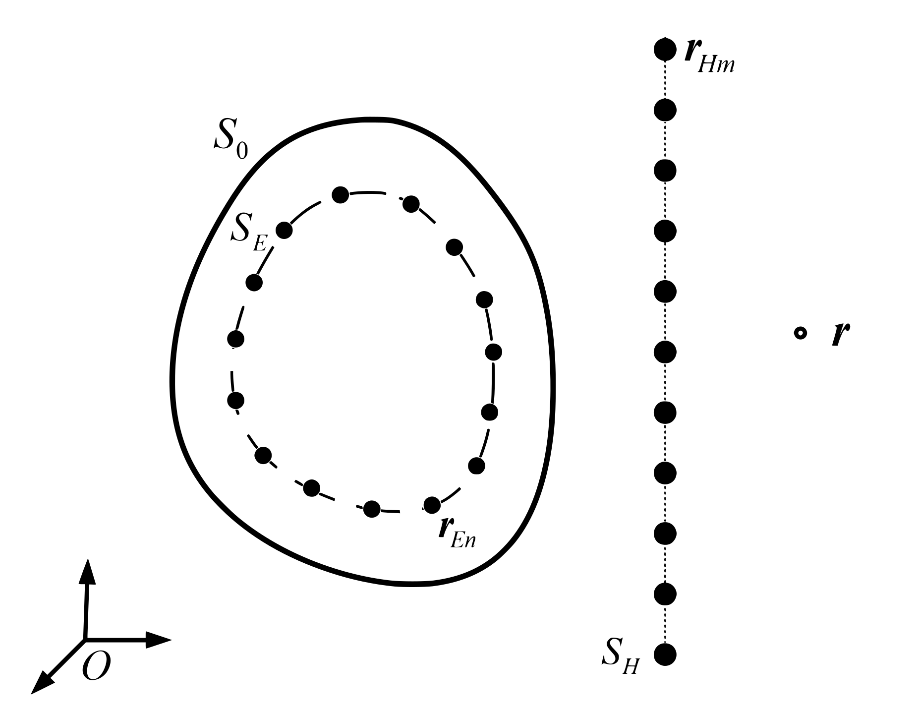
In this section, the ESM is briefly reviewed. The ESM is based on the fundamental idea that the sound field radiated by a vibrating structure can be approximated as the superposition of the sound field generated by a set of equivalent sources distributed inside the structure [29]. The equivalent source strength can be derived by matching the normal velocity of the structure surface [30], the sound pressure [31], and the particle velocity [32] of the sound field. In this paper, the equivalent source strength is calculated with the sound pressure information. A vibrating object immersed to a finite depth tends to be the same as that in infinite fluid when the submerged depth exceeds quintuple the radius [33]. The ocean interface has little influence on the measurement when the sound pressure is measured in the nearfield. Thus, the following theory is based on the free-space assumption. Considering a vibrating object in an infinite and homogeneous fluid medium, as shown in Figure 1. The sound pressure at can be expressed as follows [12].
- : the imaginary unit;
- : the density of the acoustical medium;
- : the angular frequency;
- : the mth measuring position on the measuring surface ;
- : the equivalent source on the virtual surface ;
- : the weighting factor of equivalent sources.
The function is the free-space Green’s function between and , and the time convention is omitted [6].
- k: the wavenumber;
- : the distance between and .
Equation (1) can be discretized as follows:
- N: the number of equivalent sources;
- : the source strength of the nth equivalent source.
Equation (3) can be rewritten in matrix-vector notation as
- : a vector with the measured sound pressure;
- : a vector of the equivalent source strength;
- : an matrix denoting the transfer relation between the sound pressure on the measuring surface and the equivalent source strength with the elements of .
The unknown equivalent source strength can be calculated by inverting Equation (4).
- : the generalized inverse of .
The inverse process is by nature ill conditioned, which leads to a great oscillation of the solution, also called the ill-posed problem in the numerical implementation [34,35]. The truncated singular value decomposition (TSVD) [36] can be used to eliminate the impact of the ill condition. The singular value decomposition (SVD) of the is
- : the left unitary matrix, the column vector of which is orthogonal radiation field base vector;
- : the right unitary matrix, the column vector of which is orthogonal equivalent source strength base vector;
- : a diagonal matrix whose diagonal element is singular value.
The regularized equivalent source strength can be expressed as
- : the filter factor.
The TSVD assigns some small singular values to zero. The filter factor is
- : the truncation factor.
The truncation factor can generally be determined according to the signal-to-noise ratio (SNR) in the actual sound field. The truncation factor can be set to 0.01 when the SNR in the sound field is 40 dB, as suggested in [37].
After obtaining the equivalent source strength , the sound pressure in the source-free region can be calculated:
- : the sound pressure at any point in the source-free region;
- : the transfer relation between the equivalent source strength and the sound pressure at the point .
The concrete expression of is determined by the actual acoustic environment. In addition, the particle velocity and acoustic intensity can be derived from Euler’s equation.
In summary, the solution of the ESM can be divided into two major parts. Firstly, the acoustic inverse problem is solved; that is, a set of equivalent sources are solved by matching the sound pressure information. The latter is the calculation of the acoustic forward problem; that is, the sound field is calculated using the transfer function. The strength of the equivalent source is an intermediate variable, hence the need for a suitable arrangement of the equivalent source.
2.2. Error Analysis of the ESM
Due to the effect of environmental noise, measurement position error, and inconsistency among the individual sensors in the actual measurement, errors occur when using the measured sound pressure for sound field calculation. It is can be assumed that the actual measured sound pressure on the surface is
- : the actual measured sound pressure;
- : the theoretical sound pressure;
- : the measuring error.
According to Equation (5), the relative error of is expressed as
- : the vector norm;
- cond : the condition number of a matrix.
The condition number measures the sensitivity of the solution of the linear equation system to errors in the input data [32]. Equation (11) shows that the condition number of the transfer matrix will magnify the measurement errors, which will result in a significant error of the equivalent source strength calculation. According to the operation rules of the condition number,
Therefore, the matrices , , and can be controlled to achieve the purpose of reducing the condition number of . The matrix is related to the position of the measurement point. However, in practical applications, the position of the measurement point is determined by the actual measurement array and the measurement environment, which cannot be easily changed. For , the purpose can be achieved by controlling the singular values, such as TSVD regularization. The matrix is associated with the position of the equivalent source, so the condition number of the transfer matrix can be reduced by finding a suitable position and quantity of the equivalent source.
The large condition number originates from the high column dependence in the matrix, and the position of the equivalent source determines the column elements of the transfer matrix. The transfer matrix can be rewritten as , and the coherence between the equivalent source can then be calculated with . The coherence coefficient of the transfer function is defined as
- : the complex conjugate transpose;
- : the degree of coherence between and .
When , the transfer functions and are highly linearly dependent, leading to the ill condition of the transfer matrix.
A large number of equivalent sources will not only increase the calculation burden, but produce a considerable condition number that can easily cause calculation errors. Reducing the number of equivalent sources could reduce the condition number. This would result in a sound field generated by the superposition of equivalent sources that cannot fully simulate the structural radiation sound field. Therefore, to optimize the configuration of equivalent sources, a compromise should be made to balance the ill condition of the transfer matrix and the sufficiency of simulating the sound field radiated by a structure.
2.3. Optimization of the Equivalent Source Configuration
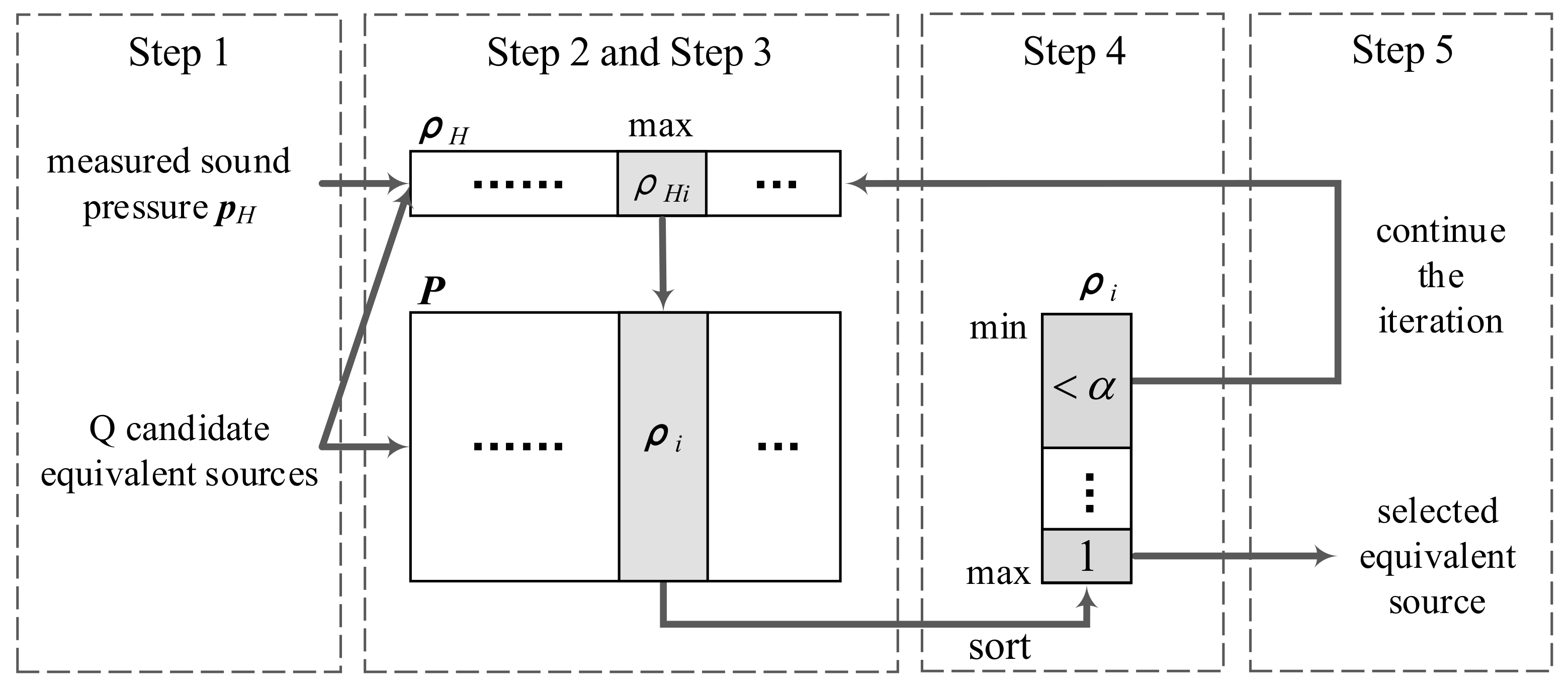
Although many studies have been conducted on the equivalent source configuration, a uniform distribution is still the mainstream method of the equivalent source configuration for practical engineering applicability and computational complexity. The method has the advantages of a simple arrangement and intuition. It still requires a large number of equivalent sources, with the issues associated with an enormous condition number. The equivalent source configuration method proposed in this paper is easy to implement, and it can determine the appropriate positions and number of equivalent sources simultaneously. The main steps of the optimization algorithm are as follows, and the flow chart of the main steps is shown in Figure 2.
- The candidate equivalent source composed of Q elements is set at a certain position on the equivalent source surface, such as the vertices of a uniform grid are distributed on the equivalent source surface. In the next steps, we select suitable equivalent sources from these candidates.
- According to Equation (13), we can calculate the coherence coefficient matrix with the column vectors of . Based on the measured sound pressure, the coherence coefficient vector with the elements of , can also be determined.
- The maximum element is found among the coherence coefficient vector , and the corresponding column vector is selected from the coherence coefficient matrix .
- Sort the elements in according to value. The candidate equivalent source corresponding to the element which is less than or equal to 1 is selected.
- Among these selected equivalent source candidates, the equivalent source equal to 1 will be retained as the equivalent source selected by the optimization algorithm. The others will be used as the input of step 2 to continue the iteration.
The optimization method is simple, and only the number of equivalent source candidates and the optimization coefficient need to be determined. The calculation error versus the number of equivalent source candidates with the same simulation condition as Section 3.1 with 1000 Hz is shown in Figure 3. As shown in Figure 3, when the number of equivalent source candidates increases to a certain degree, it has less of an impact on the optimization result. This means that the proposed method is not sensitive once the threshold number of candidates is reached. The optimization coefficient determines the coherence degree of the selected equivalent source. For large values, the ill condition of the transfer matrix is high, resulting in calculation errors. Contrarily, if reduces, the number of equivalent sources will be too small to simulate the structural radiation sound field accurately. Here, we use k-fold cross-validation, which is commonly used in machine learning [38], to determine the optimal . The procedure is as follows:
- Determine the range of according to the coherence coefficient matrix .
- Randomly divide the sound pressure measured on the measuring surface into k folds, using folds for equivalent source calculation and the other 1 fold as the calculation validation set.
- For each , substitute it into the optimization process for equivalent source calculation and then calculate the sound pressure at the corresponding position of the validation set and recording the error. This step is repeated until all the k folds are used as the validation set once.
- Repeat step 3 until all the values are used. The optimal is determined with the minimum error.
Although the optimization method, as mentioned above, is not a rigorous mathematical optimization, it has obvious advantages over the uniformly distributed equivalent source widely used in practice. The examples to follow will show that the method can use fewer equivalent sources to obtain better results.
3. Simulation and Analysis
To examine the performance of the proposed method, we performed numerical simulations. A planar baffle piston source and a cylindrical shell with spherical end-caps were employed as the radiation source examples. The uniformly distributed equivalent source will be used as a baseline for comparison with the proposed optimum distribution. In order to quantify the calculation accuracy, we define the relative error between the calculated pressure using the ESM and the theoretical pressure as follows:
- : the theoretical sound pressure in the simulation or the measured sound pressure in the experiment;
- : the calculated sound pressure using the ESM.
3.1. A Planar Baffled Piston Source
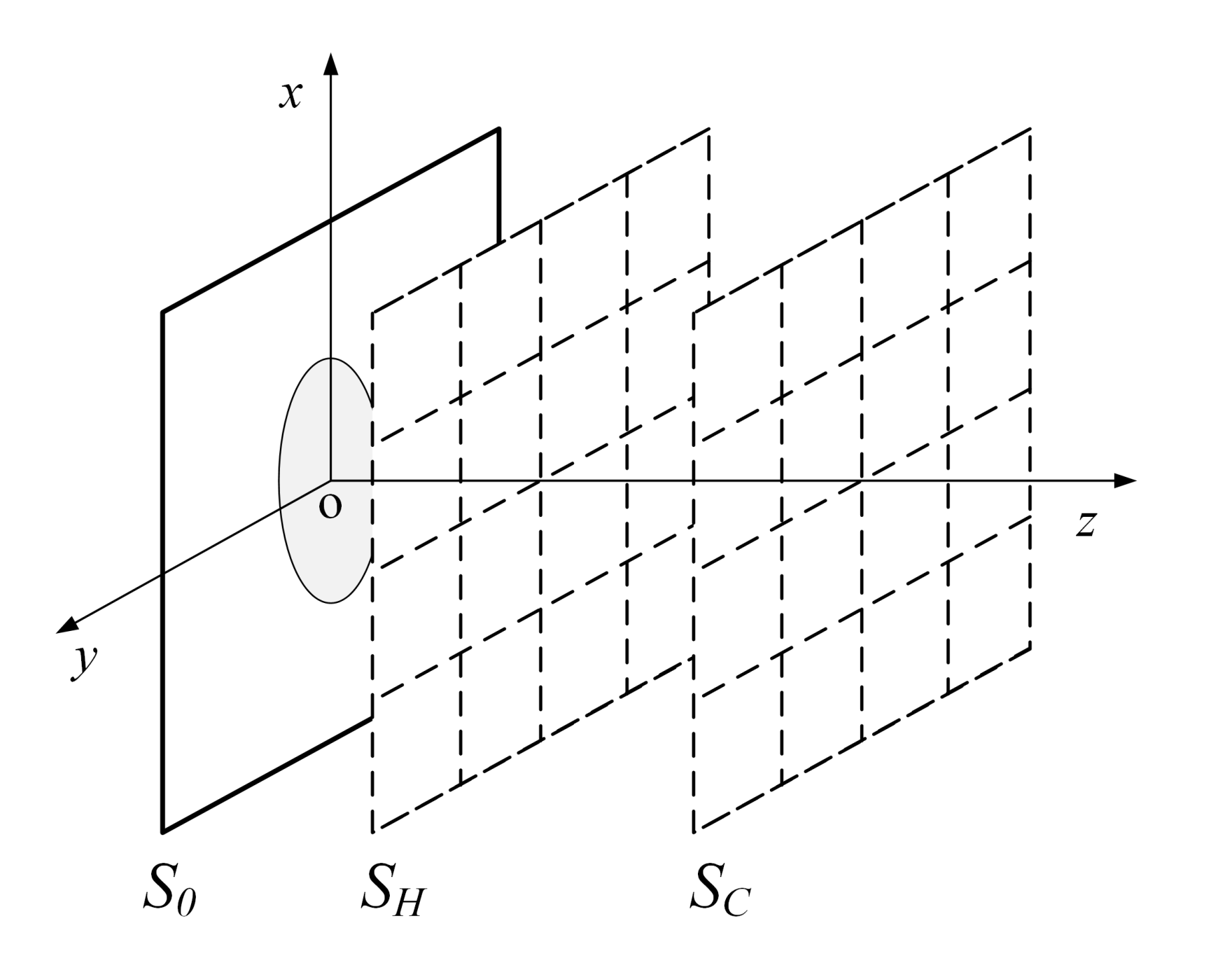
In the first numerical simulation, a planar baffled piston source [24] was used to verify the performance of the proposed method. The planar piston source was simulated by discrete point sources distributed on the plane of z = 0 m. The acoustic medium was water. The speed of sound through water was taken to be 1500 m/s, and the density of water 1000 kg/m. Suppose that the measuring plane comprises 121 measurement points uniformly distributed over an area of 2 m × 2 m with the interval of 0.2 m at z = 0.5 m. The calculation plane is located at z = 1.5 m with the same size and interval as the measuring plane, as shown in Figure 4. In the normal case, the uniformly distributed equivalent source is distributed in the same way as the measurement points on the measuring plane. The selection of the retract distance under uniform distribution refers to the previous research, as the emphasis of this paper is on the procedure of optimizing the distribution of equivalent sources on the equivalent source surface. According to [24], the plane of the equivalent source with uniform distribution is located at z = −0.09 m. The proposed method sets the source plane as the equivalent source plane. Complex Gaussian white noise with an SNR of 35 dB was added to the measured pressure to simulate the actual measurement, and the SNR is defined as .
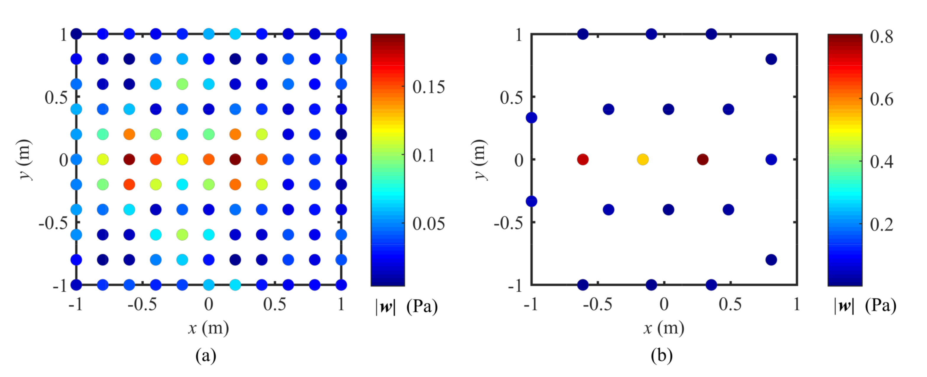
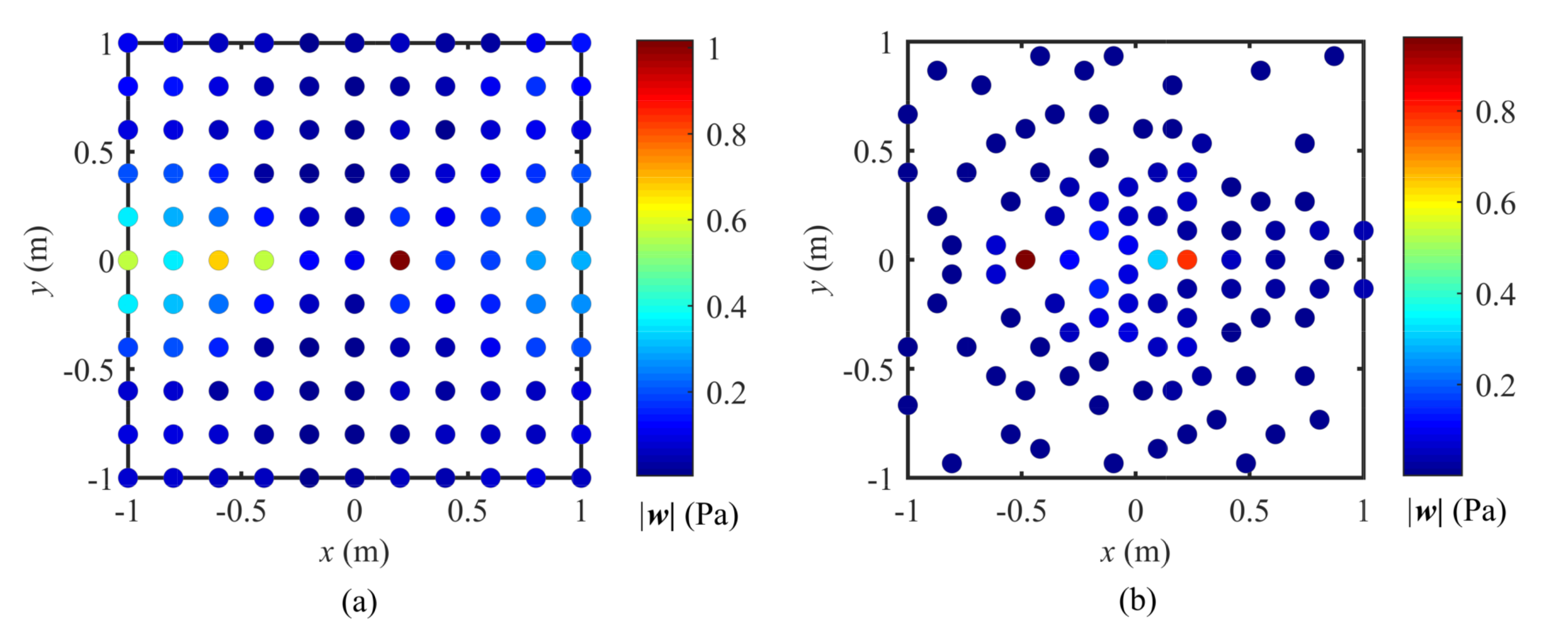
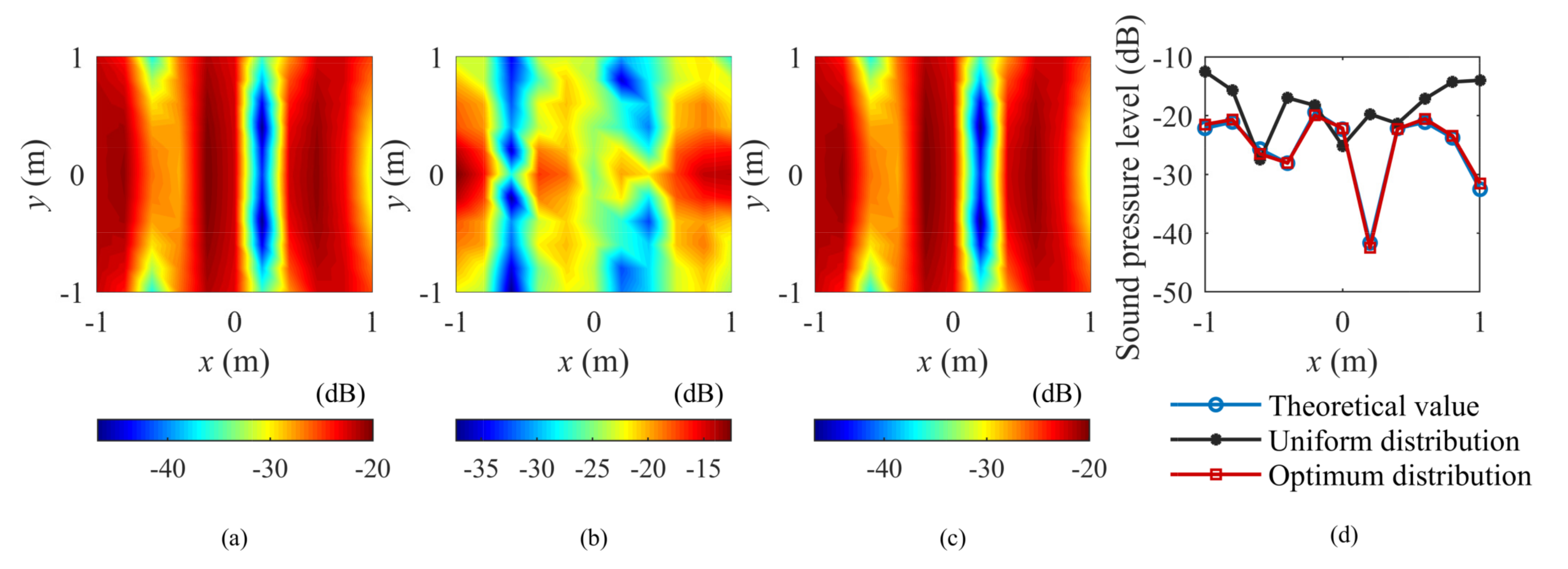
Figure 5 shows the equivalent source distribution and strength for both the uniform distribution and the optimum distribution at 1000 Hz. The color of each circle in the figure is the amplitude of the equivalent source strength . It can be seen that only 20 equivalent sources are needed after optimization compared with 121 equivalent sources of uniform distribution, which significantly reduces the number of equivalent sources. Figure 6a–c shows the computed sound pressure levels (SPL) for the two kinds of equivalent source distributions and the theoretical values on the calculation plane. For further comparison, the SPL at 11 points along the middle row of the calculation plane is shown in Figure 6d. It can be seen that, with low frequency, all methods provided good solutions that match the theoretical values well. The relative errors calculated according to Equation (14) were 2.15% and 0.58%, respectively, indicating fairly accurate calculations.
For 5000 Hz, the equivalent source distribution and strength for both distributions are shown in Figure 7. The proposed method selects more equivalent sources automatically to simulate the object radiation sound field, due to the increased frequency. Despite this, 98 equivalent sources are needed after optimization, which is still smaller than the number of uniformly distributed equivalent sources. As we can see from Figure 7b, there is an analogy between the optimization algorithm and the sound source localization method, so the locations of the discrete point sources can be found. The results of the calculated sound pressure and theoretical value at 5000 Hz are shown in Figure 8. By comparison with Figure 8d, it can be seen that the pressure calculated using the uniformly distributed equivalent sources differs largely from the theoretical value. In contrast, the proposed method gave a better solution with a smaller number of equivalent sources. The relative error of the optimum distribution was only 6.14%. In the case of uniform distribution, the relative error was 93.87%, which is much larger than that of the proposed method.
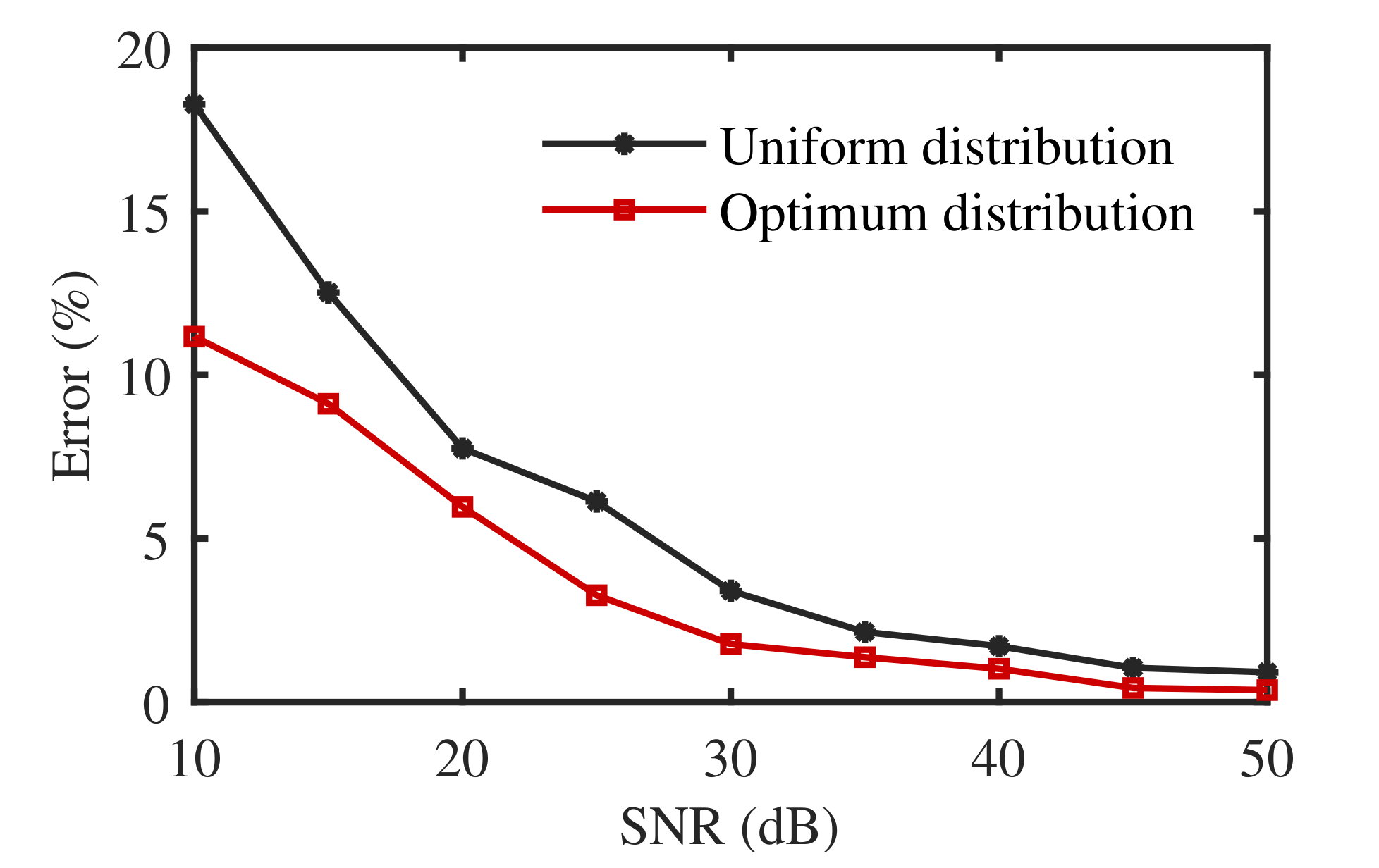
To investigate the performance of the proposed method at different SNRs, a Monte-Carlo simulation [39]—they solve the problem of statistical inference via random simulations—was used to evaluate the relative error of the calculated sound pressure. Figure 9 shows the relative error values for different SNRs using two kinds of equivalent source distributions with an SNR range of 10–50 dB at 2000 Hz. It can be seen that the relative error grossly decreases with an increasing SNR. The calculated sound field accuracy of the optimized equivalent source is higher than that of the uniformly distributed equivalent source. As long as the SNR of the measured sound pressure is higher than 20 dB, the proposed method can yield a good solution, with a relative error of less than 5%.
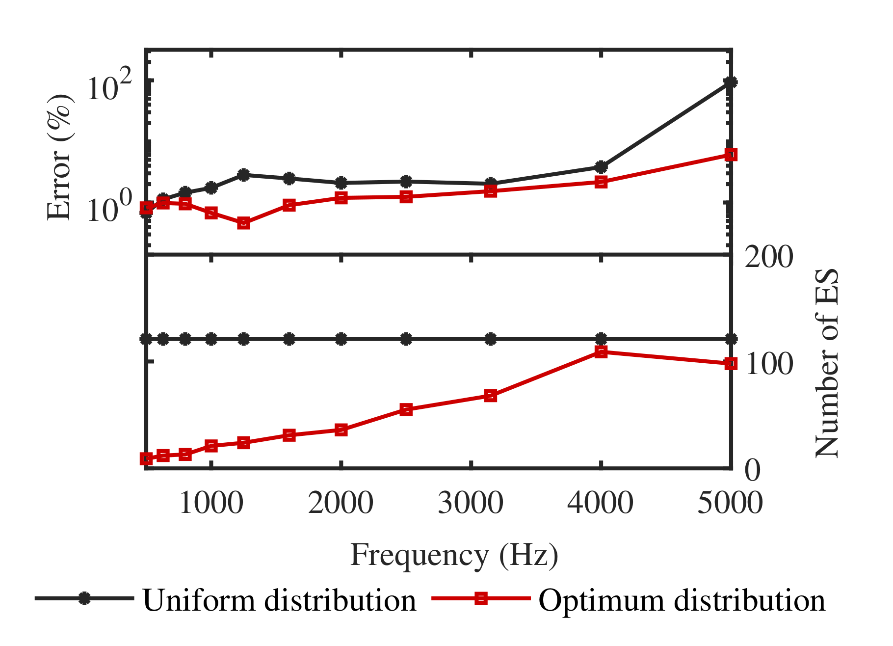
To further verify the stability of the proposed method, the relative errors of calculated sound pressure and the numbers of equivalent sources of two kinds of distribution versus frequency are shown in Figure 10. The frequency band was 500–5000 Hz (1/3 oct.). In order to better display the comparison of the low-frequency band, the logarithm axis was used for the vertical axis of relative error. It is apparent from Figure 10 that the sound pressure calculated by the optimized equivalent source was accurate over the frequency range analyzed, with a relative error of less than 10%. In the case of uniform distribution, the relative error was larger than that of the optimum distribution, especially in the high-frequency band, even being close to 100% at 5000 Hz. As the frequency increased, more equivalent sources were selected through the optimization coefficient , which was determined by the k-fold cross-validation method. Therefore, the radiated sound field was fully simulated. The optimum distribution was superior to the uniform distribution regardless of the number of equivalent sources or the calculation accuracy. This proves that the method can automatically select fewer equivalent sources to accurately calculate the sound field, significantly reducing the number of subsequent calculations, making the ESM easier to combine with other methods.
3.2. A Cylindrical Shell with Spherical End-Caps
A cylindrical shell with spherical end-caps, which accounts for a large proportion of the research on underwater structures, was used to test the performance of the proposed method. However, the radiated sound field of this structure lacks an analytical solution, and the BEM+FEM method was applied to compute the radiated pressure numerically. The cylindrical shell had a radius of 0.06 m, a total length including end-caps of 0.48 m, and a thickness of 0.002 m. The properties of steel are Young’s modulus of Pa, 7800 kg/m, and a Poisson’s ratio of 0.3. The internal medium and external medium were air and water, respectively. A point-force at the top of one hemisphere shell excites the structure vibration and radiates sound. The cylindrical model was established in Cartesian coordinates with the coordinate origin at the center of the cylinder shell. The central axis of the cylindrical shell coincided with the y-axis. In line with other studies, the uniformly distributed equivalent sources were placed on the surface, which was conformal to the structure with a retract ratio of 0.8. The measuring surface was a cylindrical surface with the center axis coinciding with the z-axis, and the radius was 0.7 m. The cylindrical shell was at the center of the cylindrical measuring surface, as shown in Figure 11. There were 12 measurement points evenly distributed in the axial direction with an interval of 0.1 m and 36 measurement points evenly distributed in the circumferential direction with an interval of 10°—a total of 432 measurement points. Complex Gaussian white noise with an SNR of 35 dB was added to the measured pressure. The surface to be calculated was a cylinder conformal to the measuring surface with a radius of 2 m.
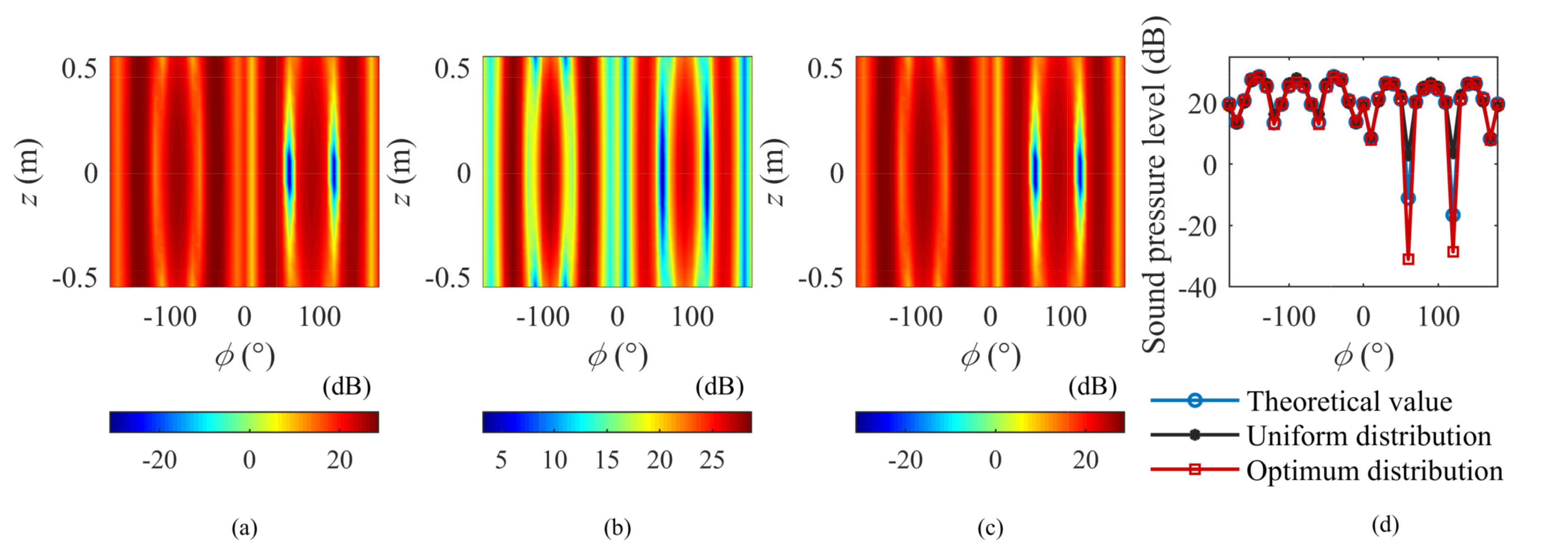
Figure 12 shows the position and strength of the equivalent source with uniform distribution and optimum distribution at 5000 Hz. It can be seen that 32 equivalent sources were needed after optimization compared with 415 equivalent sources with uniform distribution, which significantly reduced the number of equivalent sources. Figure 13 shows the SPL computed for the two kinds of equivalent source distributions and the theoretical values. As can be seen from the diagram, the uniform distribution provided effective solutions that match the theoretical value, but the proposed method got closer to the theoretical value. When the theoretical value was less than −20 dB, the computed value was not in good agreement with the theoretical value, and the calculated value was slightly larger. This was because of the influence of noise on the measuring surface. This part of the corresponding sound pressure value is small and should not produce a large calculation error. The relative errors were 0.77% and 9.05%, respectively.
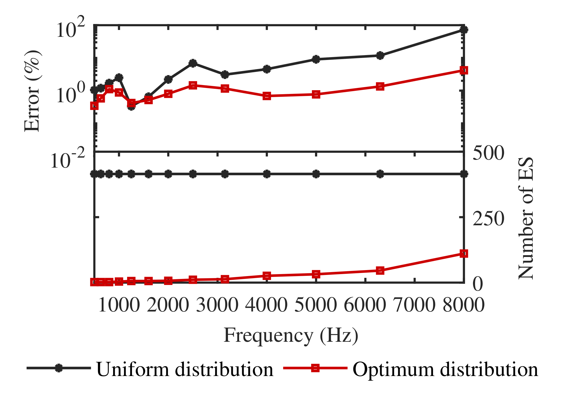
The relative error of the calculated sound pressure and the number of equivalent sources versus frequency are shown in Figure 14. The analyzed frequency band was 500–8000 Hz (1/3 oct.). The results show that, within the analyzed frequency band, in general, the calculation error increased with the frequency. The sound pressure calculated by the optimized equivalent source was accurate; relative errors were all lower than 5%. The relative error of uniform distribution increased rapidly with frequency. The greatest error was 72.46% at 8000 Hz. This indicates that the proposed method can yield good results when the calculation of uniform distribution is invalid. The number of equivalent sources required is much less than that of the uniform distribution. When the frequency was lower than 6300 Hz, the number of equivalent sources needed for optimum distribution was less than 50, which was less than 12% of the number required for uniform distribution. The simulation proved the effectiveness of the proposed method.
4. Experimental Verification
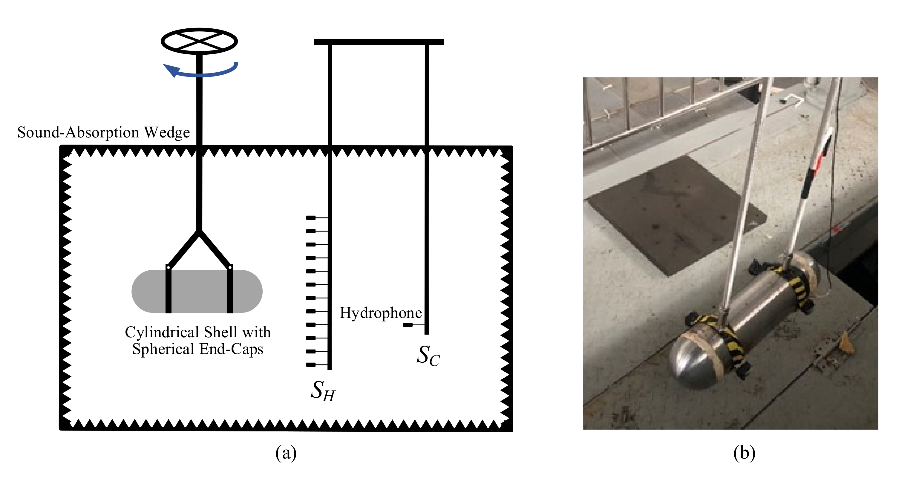
An experiment was conducted to validate the optimization algorithm. The sound source used in the experiment was the same cylindrical shell with the spherical end-cap structure introduced in Section 3.2. The cylindrical shell is excited by an exciter installed on the top of one hemisphere shell to radiate sound. Sound pressure is measured by hydrophones. The hydrophone converts the acoustic signal into an electrical signal and is used to receive the acoustic signal in the water. The hydrophone used in this experiment was an 8103, which is a commonly used scalar hydrophone. The specific parameters are shown in Table 1. The central axis of the cylindrical shell was parallel to the water surface. Restricted by experimental conditions, the scanning measurement method was used with a small array. The receiving array was a cylindrical array formed by linear array scanning. The line array was 1.1 m in length, on which 12 hydrophones were fixed on the array frame by fixture, with an equal spacing of 0.1 m. The hydrophone line array was perpendicular to the water’s surface, and the center was at the same depth as the geometric center of the cylindrical shell, with a distance of 0.45 m. In the experiment, when the rotating structure of the fixed cylindrical shell rotated one cycle, it corresponded to an entire cylindrical surface scanned by the linear array. The cylindrical shell rotated 10° each time for a total of 36 times, corresponding to 432 points scanned on the cylindrical surface. In order to obtain the measured sound pressure equivalent to a cylindrical array at the same time, a reference hydrophone was fixed near the cylindrical shell, which remained relatively stationary with the shell while the shell was rotating. In order to verify the accuracy of the sound field calculation, a hydrophone was set up 1 m from the origin as the verification point. A schematic diagram of the experimental setup and the sound source structure is shown in Figure 15. The setting of the equivalent source surface is the same as it is in the simulation. Considering the lower sound absorption limit of the anechoic pool and the applicable frequency band of exciter, the exciting frequencies were 3150, 4000, 5000, and 6300 Hz.
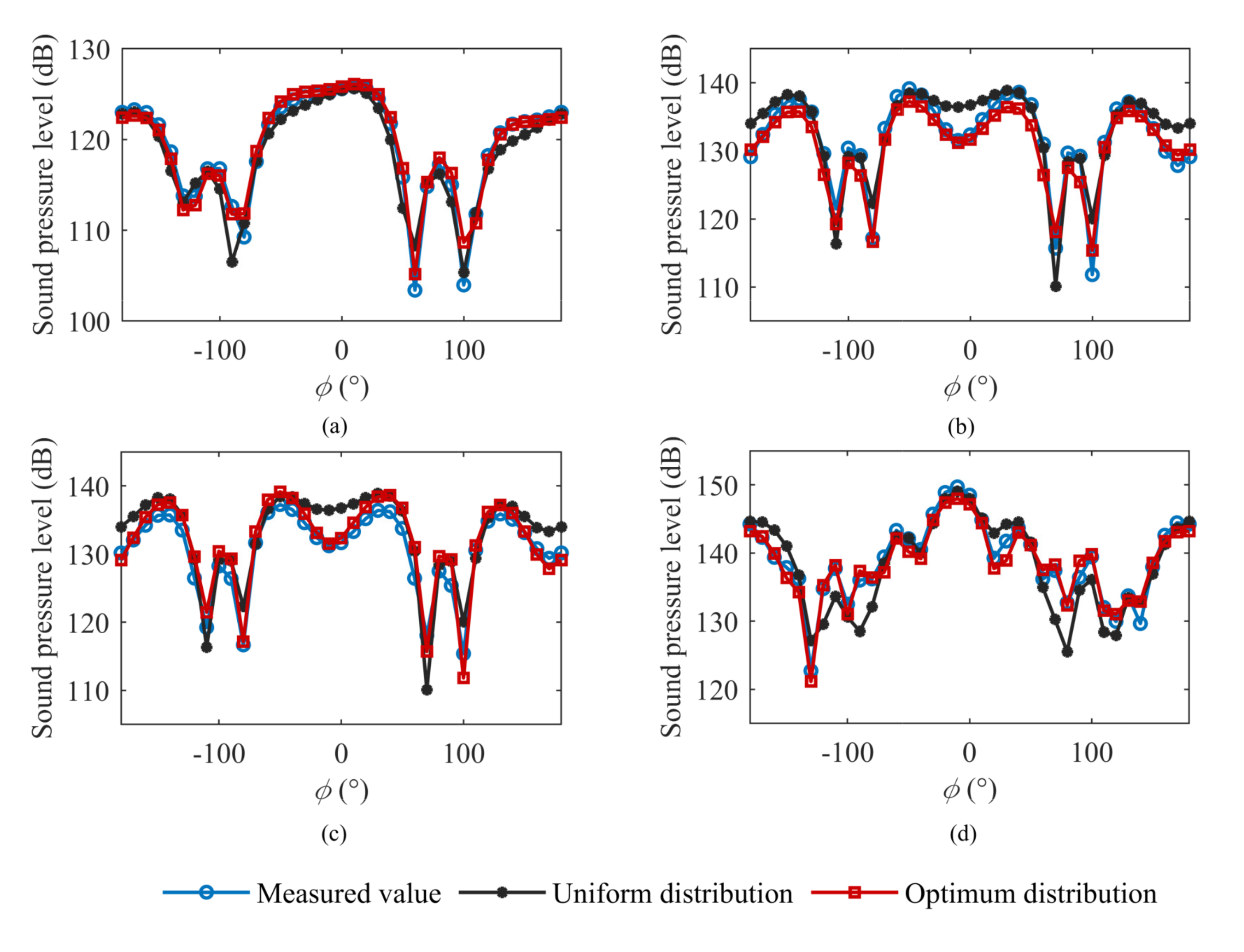
Figure 16 shows the SPL measured on the and those calculated by the ESM with two kinds of equivalent source distributions. It can be seen that the calculated SPL match the measurement in general. The fixtures of the cylindrical shell and the installation of internal exciter changed the vibration mode of the shell, resulting in different radiated sound fields from that in the simulation, but this did not affect the sound field calculation using the ESM. The relative error calculated according to Equation (14) and the numbers of equivalent sources required are given in Table 2. The relative error in the experiment results, which is larger than it was in the simulation, was caused by the scattering of the hydrophone array bracket, the error of the array element position, the inconsistency of the hydrophone, etc. Nevertheless, we can still see, by comparing the two methods, that the proposed method provided a better solution with a smaller number of equivalent sources. The proposed method selected more equivalent sources automatically to simulate the object radiation sound field with higher frequencies. The experimental results show that the selection of equivalent sources is crucial to the calculation accuracy of ESM. Compared with uniformly distributed equivalent sources, the optimized equivalent sources can be used to accurately calculate the sound field with fewer equivalent sources, confirming our previous simulation conclusion.
5. Conclusions
This paper investigated the problem of equivalent source configuration, which limits the application of ESM. The main contribution of this work is that we proposed an easy to implement and straightforward method for the equivalent source configuration, which can determine the appropriate positions and quantity of monopole equivalent sources simultaneously. In this optimization method, the coherence coefficient of the transfer function is used as a reference to balance the ill condition of the transfer matrix against the adequacy of the simulated structure radiated sound field. In numerical simulations, a planar baffled piston source and a cylindrical shell with spherical end-caps were used to examine the performance of the proposed method. The results showed that the optimization method does not yield a strict mathematical optimum of equivalent source configuration but yields more accurate sound field calculation results with fewer equivalent sources than those obtained with the uniformly distributed equivalent sources. Finally, the experiment with a cylindrical shell further confirmed the advantage of the proposed method. After optimization, the number of equivalent sources was less than 13% of equivalent sources with a uniform distribution in the analyzed frequency band. This result means that when ESM is used to calculate the radiated sound field of the structure in the marine environment, the amount of calculation will be greatly reduced. When calculating the sound propagation in a complex ocean, such as the large inclination of the seabed, the calculation step must be greatly reduced, which reduces the calculation speed. The proposed method reduces the number of cycles to calculate the ocean sound propagation to reduce the time required, which is beneficial to the realtime prediction of the structural acoustic radiation in a complex ocean. The optimized method with lesser computational demands and fewer equivalent sources will continue to be studied in future research.
Author Contributions
Conceptualization, L.Z. and D.Y.; data curation, J.W. and D.W.; formal analysis, J.W.; investigation, D.W.; methodology, J.W.; project administration, B.H.; resources, L.Z. and D.Y.; software, J.W.; supervision, L.Z. and D.Y.; validation, B.H.; writing—original draft, J.W.; writing—review and editing, L.Z. and D.Y. All authors have read and agreed to the published version of the manuscript.
Funding
This research received no external funding.
Conflicts of Interest
The authors declare no conflict of interest.
References
- Zou, M.S.; Wu, Y.S.; Liu, S.X. A three-dimensional sono-elastic method of ships in finite depth water with experimental validation. Ocean Eng. 2018, 164, 238–247. [Google Scholar] [CrossRef]
- Koopmann, G.H.; Song, L.; Fahnline, J.B. A method for computing acoustic fields based on the principle of wave superposition. J. Acoust. Soc. Am. 1989, 86, 2433–2438. [Google Scholar] [CrossRef]
- Ochmann, M. The source simulation technique for acoustic radiation problems. Acta Acust. United Acust. 1995, 81, 512–527. [Google Scholar]
- Song, L.; Koopmann, G.H.; Fahnline, J.B. Numerical errors associated with the method of superposition for computing acoustic fields. J. Acoust. Soc. Am. 1991, 89, 2625–2633. [Google Scholar] [CrossRef]
- Miller, R.D.; Moyer, E.T., Jr.; Huang, H.; Überall, H. A comparison between the boundary element method and the wave superposition approach for the analysis of the scattered fields from rigid bodies and elastic shells. J. Acoust. Soc. Am. 1991, 89, 2185–2196. [Google Scholar] [CrossRef]
- Junger, M.C.; Feit, D. Sound, Structures, and Their Interaction, 2nd ed.; MIT Press: Cambridge, MA, USA, 1986. [Google Scholar]
- Feit, D. Pressure radiated by a point-excited elastic plate. J. Acoust. Soc. Am. 1966, 40, 1489–1494. [Google Scholar] [CrossRef]
- Laulagnet, B.; Guyader, J.L. Modal analysis of a shell’s acoustic radiation in light and heavy fluids. J. Sound Vibr. 1989, 131, 397–415. [Google Scholar] [CrossRef]
- Everstine, G.C. Finite element formulatons of structural acoustics problems. Comput. Struct. 1997, 65, 307–321. [Google Scholar] [CrossRef]
- Bai, M.R. Application of BEM (boundary element method)-based acoustic holography to radiation analysis of sound sources with arbitrarily shaped geometries. J. Acoust. Soc. Am. 1992, 92, 533–549. [Google Scholar] [CrossRef] [Green Version]
- Chen, L.H.; Schweikert, D.G. Sound radiation from an arbitrary body. J. Acoust. Soc. Am. 1963, 35, 1626–1632. [Google Scholar] [CrossRef]
- Fernandez-Grande, E.; Xenaki, A.; Gerstoft, P. A sparse equivalent source method for near-field acoustic holography. J. Acoust. Soc. Am. 2017, 141, 532–542. [Google Scholar] [CrossRef] [PubMed]
- Valdivia, N.P.; Williams, E.G. Study of the comparison of the methods of equivalent sources and boundary element methods for near-field acoustic holography. J. Acoust. Soc. Am. 2006, 120, 3694–3705. [Google Scholar] [CrossRef] [PubMed]
- Zou, M.S.; Liu, S.X.; Jiang, L.W.; Huang, H. A mixed analytical-numerical method for the acoustic radiation of a spherical double shell in the ocean-acoustic environment. Ocean Eng. 2020, 199, 107040. [Google Scholar] [CrossRef]
- Huang, H.; Zou, M.S.; Jiang, L.W. Study on the integrated calculation method of fluid–structure interaction vibration, acoustic radiation, and propagation from an elastic spherical shell in ocean acoustic environments. Ocean Eng. 2019, 177, 29–39. [Google Scholar] [CrossRef]
- Bobrovnitskii, Y.I.; Tomilina, T.M. General properties and fundamental errors of the method of equivalent sources. Acoust. Phys. 1995, 41, 649–660. [Google Scholar]
- Gounot, Y.J.R.; Musafir, R.E. Simulation of scattered fields: Some guidelines for the equivalent source method. J. Sound Vibr. 2011, 330, 3698–3709. [Google Scholar] [CrossRef]
- Pavić, G. A technique for the computation of sound radiation by vibrating bodies using multipole substitute sources. Acta Acust. United Acust. 2006, 92, 112–126. [Google Scholar]
- Rossing, T.D. Springer Handbook of Acoustics, 2nd ed.; Springer: New York, NY, USA, 2015. [Google Scholar]
- Jensen, F.; Kuperman, W.; Porter, M.; Schmidt, H. Computational Ocean Acoustics, 2nd ed.; Springer: New York, NY, USA, 2011. [Google Scholar]
- Zhang, C.; Liu, Y.; Shang, D.; Khan, I.U. A Method for Predicting Radiated Acoustic Field in Shallow Sea Based on Wave Superposition and Ray. Appl. Sci. 2020, 10, 917. [Google Scholar] [CrossRef] [Green Version]
- Shang, D.J.; Qian, Z.W.; He, Y.A.; Xiao, Y. Sound radiation of cylinder in shallow water investigated by combined wave superposition method. Acta Phys. Sin. 2018, 67. [Google Scholar] [CrossRef]
- Jeans, R.; Mathews, I.C. The wave superposition method as a robust technique for computing acoustic fields. J. Acoust. Soc. Am. 1992, 92, 1156–1166. [Google Scholar] [CrossRef]
- Bai, M.R.; Chen, C.C.; Lin, J.H. On optimal retreat distance for the equivalent source method-based nearfield acoustical holography. J. Acoust. Soc. Am. 2011, 129, 1407–1416. [Google Scholar] [CrossRef] [PubMed]
- Pavić, G. An engineering technique for the computation of sound radiation by vibrating bodies using substitute sources. Acta Acust. United Acust. 2005, 91, 1–16. [Google Scholar]
- Gounot, Y.J.; Musafir, R.E. On appropriate equivalent monopole sets for rigid body scattering problems. J. Acoust. Soc. Am. 2007, 122, 3195–3205. [Google Scholar] [CrossRef] [PubMed]
- Gounot, Y.J.R.; Musafir, R.E. Genetic algorithms: A global search tool to find optimal equivalent source sets. J. Sound Vibr. 2009, 322, 282–298. [Google Scholar] [CrossRef]
- Jing, W.Q.; Wu, H.; Nie, J.Q. Optimization of Equivalent Source Configuration for an Independent-Equivalent Source Method in Half-Space Sound Field. Shock Vib. 2020, 2020, 6029393. [Google Scholar] [CrossRef]
- Bi, C.X.; Chen, X.Z.; Chen, J.; Zhou, R. Nearfield acoustic holography based on the equivalent source method. Sci. China Ser. E Technol. Sci. 2005, 48, 338–354. [Google Scholar] [CrossRef]
- Song, L.; Koopmann, G.H.; Fahnline, J.B. Active control of the acoustic radiation of a vibrating structure using a superposition formulation. J. Acoust. Soc. Am. 1991, 89, 2786–2792. [Google Scholar] [CrossRef]
- Bi, C.X.; Chen, X.Z.; Chen, J. Sound field separation technique based on equivalent source method and its application in nearfield acoustic holography. J. Acoust. Soc. Am. 2008, 123, 1472–1478. [Google Scholar] [CrossRef]
- Zhang, Y.B.; Jacobsen, F.; Bi, C.X.; Chen, X.Z. Near field acoustic holography based on the equivalent source method and pressure-velocity transducers. J. Acoust. Soc. Am. 2009, 126, 1257–1263. [Google Scholar] [CrossRef] [Green Version]
- Guo, W.; Li, T.; Zhu, X.; Miao, Y.; Zhang, G. Vibration and acoustic radiation of a finite cylindrical shell submerged at finite depth from the free surface. J. Sound Vibr. 2017, 393, 338–352. [Google Scholar] [CrossRef]
- Tikhonov, A.N. On the stability of inverse problems. Dokl. Akad. Nauk SSSR 1943, 39, 195–198. [Google Scholar]
- Tikhonov, A.N. On the solution of ill-posed problems and the method of regularization. Dokl. Akad. Nauk SSSR 1963, 151, 501–504. [Google Scholar]
- Demmel, J.W. Applied Numerical Linear Algebra; SIAM: Philadelphia, PA, USA, 1997. [Google Scholar]
- Chen, X.Z.; Bi, C.X. Near-Field Acoustical Holography and Its Application; Science Press: Beijing, China, 2013. [Google Scholar]
- Bengio, Y.; Grandvalet, Y. No unbiased estimator of the variance of k-fold cross-validation. J. Mach. Learn. Res. 2004, 5, 1089–1105. [Google Scholar]
- Bonate, P.L. A brief introduction to Monte Carlo simulation. Clin. Pharmacokinet. 2001, 40, 15–22. [Google Scholar] [CrossRef] [PubMed]
Figure 1.
The schematic diagram of the ESM. is the surface of the vibrating object, is the virtual surface of the equivalent source, and is the measuring surface. is the mth measuring position on the , is the nth equivalent source on the , and is a point in the source-free region.
Figure 1.
The schematic diagram of the ESM. is the surface of the vibrating object, is the virtual surface of the equivalent source, and is the measuring surface. is the mth measuring position on the , is the nth equivalent source on the , and is a point in the source-free region.

Figure 2.
The flow chart of the optimization algorithm.

Figure 3.
The relative error versus the number of equivalent source candidates.

Figure 4.
Scenarios of array distribution for simulating the planar baffled piston source. is the plane of planar baffled piston source, is the measuring plane, and is the calculation plane.
Figure 4.
Scenarios of array distribution for simulating the planar baffled piston source. is the plane of planar baffled piston source, is the measuring plane, and is the calculation plane.

Figure 5.
The position and the strength of the equivalent source at 1000 Hz: (a) uniform distribution and (b) optimum distribution.
Figure 5.
The position and the strength of the equivalent source at 1000 Hz: (a) uniform distribution and (b) optimum distribution.

Figure 6.
The SPL computed at 1000 Hz: (a) the theoretical value, (b) the value computed by the uniform distribution, (c) the value computed by the optimum distribution, and (d) the SPL along the middle row.
Figure 6.
The SPL computed at 1000 Hz: (a) the theoretical value, (b) the value computed by the uniform distribution, (c) the value computed by the optimum distribution, and (d) the SPL along the middle row.

Figure 7.
The position and the strength of the equivalent source at 5000 Hz: (a) uniform distribution and (b) optimum distribution.
Figure 7.
The position and the strength of the equivalent source at 5000 Hz: (a) uniform distribution and (b) optimum distribution.

Figure 8.
The SPL computed at 5000 Hz: (a) the theoretical value, (b) the value computed by the uniform distribution, (c) the value computed by the optimum distribution, and (d) the SPL along the middle row.
Figure 8.
The SPL computed at 5000 Hz: (a) the theoretical value, (b) the value computed by the uniform distribution, (c) the value computed by the optimum distribution, and (d) the SPL along the middle row.

Figure 9.
The relative error versus SNR at 2000 Hz.

Figure 10.
The relative error of the sound pressure (top) and the number of equivalent sources (ES) (bottom) versus frequency.
Figure 10.
The relative error of the sound pressure (top) and the number of equivalent sources (ES) (bottom) versus frequency.

Figure 11.
The spatial position relationship between the cylindrical shell with spherical end-caps, the measuring surface, and the calculation surface. is the surface of the cylindrical shell, is the measuring surface, and is the calculation surface.
Figure 11.
The spatial position relationship between the cylindrical shell with spherical end-caps, the measuring surface, and the calculation surface. is the surface of the cylindrical shell, is the measuring surface, and is the calculation surface.

Figure 12.
The position and the strength of the equivalent source at 5000 Hz: (a) uniform distribution and (b) optimum distribution.
Figure 12.
The position and the strength of the equivalent source at 5000 Hz: (a) uniform distribution and (b) optimum distribution.

Figure 13.
The SPL computed at 5000 Hz: (a) the theoretical value, (b) the value computed by the uniform distribution, (c) the value computed by the optimum distribution, and (d) the SPL along the middle row.
Figure 13.
The SPL computed at 5000 Hz: (a) the theoretical value, (b) the value computed by the uniform distribution, (c) the value computed by the optimum distribution, and (d) the SPL along the middle row.

Figure 14.
The relative error of the sound pressure (top) and the number of equivalent sources (bottom) versus frequency.
Figure 14.
The relative error of the sound pressure (top) and the number of equivalent sources (bottom) versus frequency.

Figure 15.
(a) The schematic diagram of experimental setup. is the measuring surface and is the verification point. (b) The photo of cylindrical shell used in the experiment.
Figure 15.
(a) The schematic diagram of experimental setup. is the measuring surface and is the verification point. (b) The photo of cylindrical shell used in the experiment.

Figure 16.
A comparison of the measured values and the computed SPL. Frequencies: (a) 3150 Hz, (b) 4000 Hz, (c) 5000 Hz, and (d) 6300 Hz.
Figure 16.
A comparison of the measured values and the computed SPL. Frequencies: (a) 3150 Hz, (b) 4000 Hz, (c) 5000 Hz, and (d) 6300 Hz.


Table 1.
The hydrophone parameters.
| Type | Length | Diameter | Voltage Sensitivity | Frequency Response |
|---|---|---|---|---|
| 8103 | 50 mm | 9.5 mm | −211 dB re 1 V/Pa | 0.1 Hz to 20 kHz: +1 dB, −1.5 dB |
Table 2.
The relative errors and the numbers of equivalent sources for sound field calculations.
| Frequency (Hz) | Relative Error (%) | Number of Equivalent Sources | ||
|---|---|---|---|---|
| Uniform Distribution | Optimum Distribution | Uniform Distribution | Optimum Distribution | |
| 3150 | 16.64 | 8.31 | 415 | 27 |
| 4000 | 40.55 | 24.03 | 415 | 27 |
| 5000 | 38.9 | 21.43 | 415 | 38 |
| 6300 | 38.53 | 26.19 | 415 | 53 |
Publisher’s Note: MDPI stays neutral with regard to jurisdictional claims in published maps and institutional affiliations. |
© 2021 by the authors. Licensee MDPI, Basel, Switzerland. This article is an open access article distributed under the terms and conditions of the Creative Commons Attribution (CC BY) license (https://creativecommons.org/licenses/by/4.0/).
Share and Cite
MDPI and ACS Style
Zhang, L.; Wang, J.; Yang, D.; Hu, B.; Wu, D. Optimization of the Equivalent Source Configuration for the Equivalent Source Method. J. Mar. Sci. Eng. 2021, 9, 807. https://doi.org/10.3390/jmse9080807
AMA Style
Zhang L, Wang J, Yang D, Hu B, Wu D. Optimization of the Equivalent Source Configuration for the Equivalent Source Method. Journal of Marine Science and Engineering. 2021; 9(8):807. https://doi.org/10.3390/jmse9080807
Chicago/Turabian StyleZhang, Lanyue, Jia Wang, Desen Yang, Bo Hu, and Di Wu. 2021. "Optimization of the Equivalent Source Configuration for the Equivalent Source Method" Journal of Marine Science and Engineering 9, no. 8: 807. https://doi.org/10.3390/jmse9080807
Note that from the first issue of 2016, this journal uses article numbers instead of page numbers. See further details here.