
The Effect of Mean-Reverting Processes in the Pricing of Options in the Energy Market: An Arithmetic Approach

1
Center for Mathematical Economics, Bielefeld University, 33615 Bielefeld, Germany
2
Independent Researcher, 51065 Cologne, Germany
*
Author to whom correspondence should be addressed.
†
These authors contributed equally to this work.
Risks 2021, 9(5), 100; https://doi.org/10.3390/risks9050100
Submission received: 5 April 2021
/
Revised: 1 May 2021
/
Accepted: 7 May 2021
/
Published: 18 May 2021
(This article belongs to the Special Issue Stochastic Modeling and Pricing in Energy Markets)
Abstract
:In this paper we study the effect that mean-reverting components in the arithmetic dynamics of electricity spot price have on the price of a call option on a swap. Our model allows for seasonal effects, spikes, and negative values of the price of electricity. We show that for sufficiently large delivery periods of the swap contract, the error that one makes by neglecting some of the mean-reverting processes affecting the spot price evolution converges to zero. The decay rate is explicitly calculated. This is achieved by exploiting the additive structure of the electricity price process in order to determine an explicit closed-form formula for the price of the call on a swap. The theoretical analysis is then illustrated via a numerical example.
1. Introduction
Deregulation of energy markets started in the early 1990s, with the main aim being making energy markets more efficient and reducing costs for the consumer (see Al-Sunaidy and Green (2006) for a detailed discussion on the history of deregulation). Today, energy is traded under free market conditions in many countries, and energy prices show characteristics that are rarely seen in other markets. These are, for example, seasonal effects, jumps with fast mean-reversion, and negative prices, and a large number of models have been produced in the recent years in order to capture those features and investigate their structure; see, among many others, Borovkova and Schmeck (2017); Fanelli and Schmeck (2019); Genoese et al. (2010); Kaminski (2013); Kiesel et al. (2009), as well as the recent review Deschatre et al. (2021).
Considerations involving the law of demand and supply can explain the presence in electricity prices of seasonal patters at different scales: Prices are typically higher during the morning and evening hours of the days, and—especially in countries where heating is performed via electricity—also in winter months. Since these seasonal patterns are predictable, they can be well described through deterministic time-dependent functions, such as a combination of different sinusoidal functions (Escribano et al. 2011). Energy prices show very high volatility with jumps, which can be explained by the fact that energy cannot be stored on a large scale, at least in an economically feasible way. Furthermore, a large energy supply combined with a low demand leads electricity prices also to become negative, a feature allowed since 2008 by the European Energy Exchange. As a matter of fact, in periods of overproduction a shut down of the power plants would cost the energy producers more than paying for getting rid of energy.
From a mathematical point of view, there are clearly various modeling choices for electricity spot prices; see the reviews Weron (2014) and Deschatre et al. (2021) for an outlook on the state of the art and future perspectives. Following the seminal work by Benth et al. (2007), in this paper we choose to work with a (nowadays classical) multi-factor spot price model consisting of a non-stationary process and a sum of independent Ornstein-Uhlenbeck processes, driven by a suitable stochastic jump process. Namely, we take the spot price of electricity given by
for some index-set J. Here, is a deterministic seasonality function, X is an arithmetic Brownian motion that reflects long term expectations, e.g., of political developments, and each is a mean-reverting process, that converges back to the seasonal equilibrium level . On the one hand, as we shall see also in this paper, this modeling choice is still simple enough to enable for explicit evaluations of electricity contracts (like futures and forward contracts). On the other hand, Equation (1) allows to reproduce the well-known stylized fact for which electricity prices exhibit large price shocks (spikes), which mean revert very fast towards the original price level, as well as slower mean reverting components. As a matter of fact, Meyer-Brandis and Tankov (2008) find that the majority of European exchanges show an auto-correlating structure of the spot prices that can be well described by a models including a sum of mean reverting processes, where the mean reversion takes place with different rates. In particular, Meyer-Brandis and Tankov (2008) argue that two or three mean reverting factors are suitable to reproduce prices in the EEX.
However, Ball and Torous (1983) and Knittel and Roberts (2001), among others, also point out the difficulty of calibrating a multi-factor spot price model as in Equation (1) to market data. Indeed, the question arises of how to filter from the observed time series the different, themselves not observable, components. It is therefore natural to investigate which is the error that one makes by neglecting some or all of the mean-reverting processes in the spot price model. In particular, if such an error is shown to be relatively small, then it might not be worth to provide the nontrivial calibration of a full jump model of electricity prices. In this paper we interpret such a question by comparing the price of vanilla options on swaps in two models for S. In a first one all the mean-reverting components are considered, and in a second one only jump Ornstein-Uhlenbeck processes are considered. Our main result gives an analytical estimate of the pricing error by showing that the difference in the price of call options on swaps for the two models can be bounded from above and below by explicitly calculated quantities. These depend on the models’ parameters, such as the volatility parameters, the speeds of mean-reversion, and the delivery period in the swap pricing formula. We show that when the delivery period is sufficiently large, then the pricing error goes to zero. This is because the swap averages out the effects that spikes have on the call option price. We thus conclude that for sufficiently long delivery periods, considering a relatively less complex spot price model provides a good approximation to the more complex one. Our theoretical analysis is then illustrated by numerical examples. Here we show the effect of the mean-reverting components and of the volatility of the non-stationary component on the price of call options. In particular, we confirm that for relatively large delivery periods of the swap contract the pricing error is negligible. Furthermore, we observe that the smaller is, the larger becomes the pricing error.
Our study is related to the one performed in Benth and Schmeck (2014) and Schmeck (2016) (see also Nomikos and Soldatos (2010) for a study of the importance of mean reversion and spikes in the stochastic behavior of the underlying asset when pricing options on power). The main difference between Benth and Schmeck (2014) and Schmeck (2016) and our paper lie in the structure of the dynamics of the spot price process. These are geometric in Schmeck (2016), while arithmetic in this work. The choice of considering an arithmetic model has essentially two main reasons. First of all, arithmetic dynamics allow to encompass the observed negativity of spot prices of electricity. The importance of taking into account such a stylized fact of electricity prices in the modeling is also confirmed by the increasing interest that arithmetic models are recently obtaining in the literature (see, e.g., Benth et al. 2019; Edoli et al. 2017; Fanone et al. 2013; Hinderks and Wagner 2020; Latini et al. 2019; Piccirilli et al. 2021). Second of all, using arithmetic models one can obtain explicit closed form formulas for the price of the swap price, given by the time-average of the spot price over the delivery period. This is not possible for geometric models, such that Benth and Schmeck (2014) and Schmeck (2016) approximate the delivery period by its midpoint.
The rest of this paper is organized as follows. In Section 2 we provide the spot price dynamics and derive the dynamics of the swap price. In Section 3 we then determine the price of the call option on the swap, which is then employed in Section 4 in order to estimate the pricing error obtained by neglecting jump mean-reverting components in the spot price evolution. Finally, Section 5 illustrates the theoretical analysis by numerical examples.
2. Setting
In this section, we define the financial setting within which we will perform our study. In particular, in the following we will define the dynamics of the spot price of electricity and derive the price of a swap contract and its corresponding time evolution.
2.1. Spot Price Dynamics
Consider a filtered probability space , satisfying the usual conditions. As we are interested in the option price, we state here the spot price dynamics already under a suitable pricing measure . Then, letting J be an index set with cardinality , for any the spot price of electricity is assumed to evolve as
Here is a deterministic function; X is given by
for some , some deterministic function , and for a one-dimensional Brownian motion B. Furthermore, for any , is a mean-reverting process with dynamics
where we set
for a Poisson process with time-dependent intensity . As in Geman and Roncoroni (2006), a time-dependent intensity accounts for the seasonality in the arrival of spikes. Furthermore, in Equation (4), are independent one-dimensional Brownian motions. Note that, due to the presence in each of all the vector of Brownian motions , the mean-reverting processes are clearly correlated. The random variables are all independent of each other, and for any they are identically distributed with density functions . The family determines the (random) sizes of the jumps of the compound-Poisson processes .
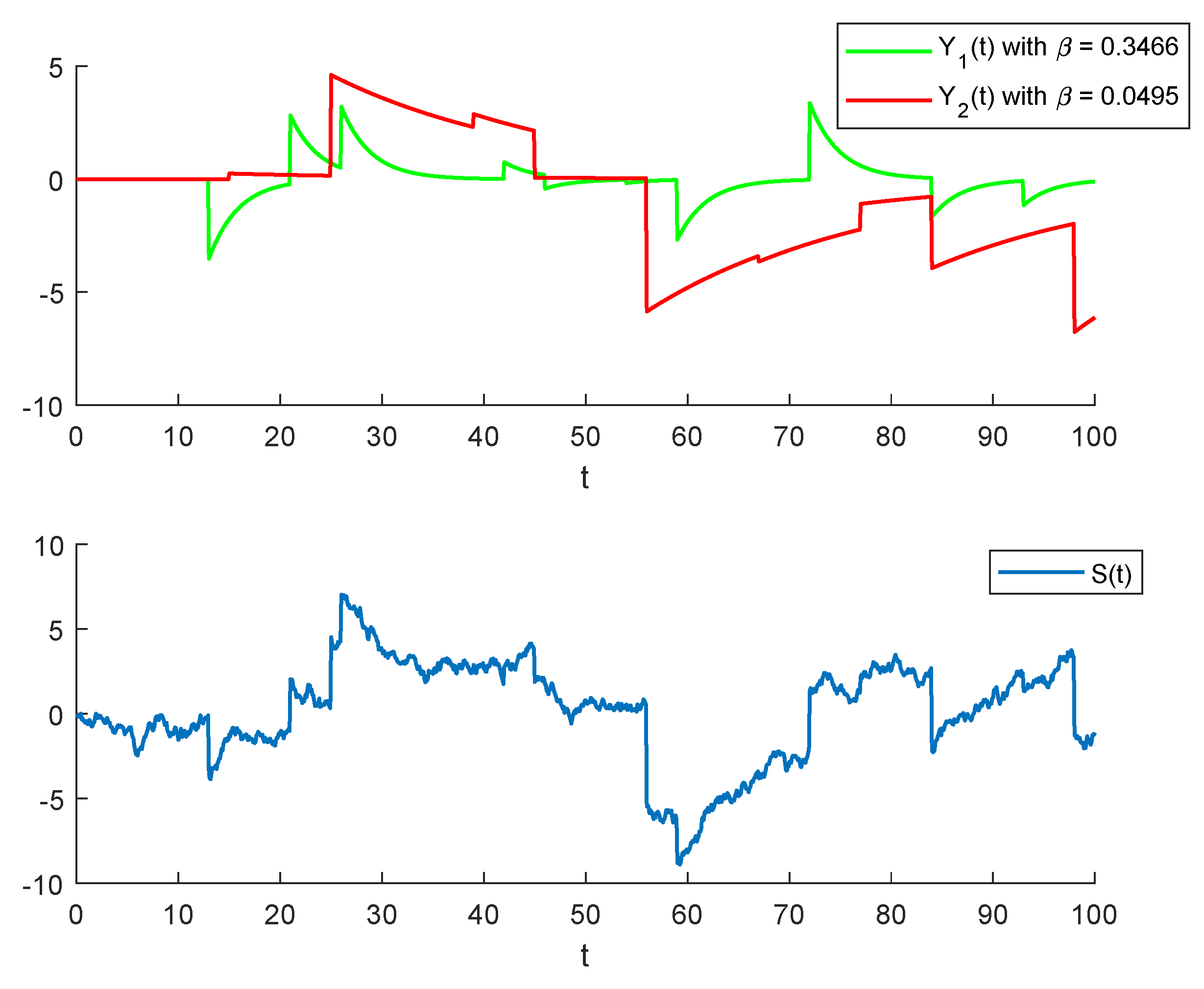
An illustration of a sample path of the mean-reverting processes , , as well of the spot price S are provided in Figure 1 below. In the first drawing, we take and, in order to better illustrate the role of mean-reversion, the two mean-reverting processes and are of pure-jump-type (i.e., for all ). We observe that, after each jump, —which has an higher mean-reversion speed—tends towards the equilibrium level 0 much faster than . In the second drawing, we observe a sample path of the spot price which, according to Equation (2), is given by the sum of the mean-reverting dynamics and of the Brownian term X (for simplicity, we are taking ).
Throughout this paper we make the following standing assumption.
Assumption A1.
For any and we have that . Moreover, the processes and the random variables are all assumed to be independent of each other.
In Equation (2), is a deterministic seasonality function. For example, this could be modeled as a combination of sine functions as in Escribano et al. (2011). On the other hand, the drifted Brownian motion X simulates the randomly fluctuating long-term trend of the spot price, while the mean-reverting processes take care of the observed mean-reverting jump-component of the spot price. Notice that, differently to Schmeck (2016), among others, in our specification the price process can become negative due to the arithmetic structure of the considered dynamics. This is in line with the observation of negative prices of electricity. Moreover, the fact that we consider a family of mean-reverting processes allows us to model different mean-reversion rates for the spot price. The speeds of mean-reversion , as well as the volatilities and , are assumed to be time-dependent in order to accommodate for possible seasonal effects. From now on we will assume that those deterministic functions are bounded and nonnegative.
2.2. Swap-Price Value and Dynamics
Call options in the energy market are usually written on swaps that deliver the energy over a contracted period (Options Trading at EEX 2018). Here, is the starting time of the delivery period and is the end of the delivery period. During this horizon, the buyer of such a contract has to pay a fixed price per MWh. These kind of contracts are called swap contracts and their price is usually evaluated under some measure , equivalent to . However, due to the non-storability of electricity, does not need to be a martingale measure for the spot. Then, by Chapter 4 in Benth et al. (2008), we have that the swap price at time t is given by the expected average spot price over the delivery period, given all the information available at the current instant:
The next result provides an explicit computation of F within our model. Its proof easily adapts arguments from Benth et al. (2008) to our additive setting, and we provide details in Appendix A for the sake of completeness. This preliminary result will be needed in Section 4 below in order to derive the main result of this paper, namely the explicit error bounds obtained in Theorem 4.
Theorem 1.
Let and the spot price be given as in Equation (2). Then the price of the swap is given by:
The next result provides the dynamics of .
Theorem 2.
Let the spot price be given as in Equation (2). Then, for any , the dynamics of the swap are given by:
where
is a compensated Poisson process.
The proof can be found in Appendix A.
3. Pricing a Call Option on the Swap
In this section, we are going to calculate the fair price of a call option that is written on a swap. Notice that such a pricing can be performed under the measure used for pricing the swaps. Indeed, from the very definition Equation (6), as well as from the fact that the compensated jump process in Equation (8) is a -martingale, we can see that the swap price is a -martingale.
Because in Section 4 we shall study the effect of mean-reversion components on a call option price that is written on a swap F, it is useful from now on to stress that the spot and swap prices depend on these mean-reverting components. This is done in the following way: For any index set , with cardinality , we parametrize the swap price and spot price by L by assuming that only of the mean-reverting components in Equation (2) affect the dynamics of the spot price, and we write
Then, we define accordingly
and the fair price at time of a call option with maturity , underlying , and strike price , is
From Equation (12) can be decomposed as
where the continuous part is defined as
while the jump component is
It is clear that . On the other hand, by Itô’s isometry and the independence of the Brownian motions one obtains
where we have set
These distributional properties of will be used in the next theorem, which provides a formula for the fair price of the considered call option. Throughout the rest of this paper, denotes the cumulative standard normal distribution function.
Theorem 3.
Let and . Let the spot price be given as in Equation (9) and the swap be defined by Equation (10). Then, the fair price of the call option as in Equation (11) is given by
where
and
Proof.
By combining Equations (11) and (12), we find
with given as in Equation (20) and defined through Equation (13). Because the stochastic integrals are independent of we obtain from the latter
Then, by the tower property and the assumed independence of the Brownian motions with respect to the Poisson processes, we can write from Equation (22)
In order to complete the proof it thus remains only to evaluate of Equation (24). Denoting by Z a random variable with standard Normal distribution, and recalling that (Equations (14) and (16)) we find
Then, standard calculations lead for any to
where we have set
Considerations on the Effect of the Jump Components’ Volatilities
Notice that the expression of the call price in Equation (18) is consistent with the classical fair pricing formula in the Bachelier model, as expected (see Musiela and Rutkowski (1997) for a review of the Bachelier model). The main difference lies in the fact that the coefficient in Equation (18) depends on the jump-components of the spot price dynamics. However, from Equation (18) it is not clear how those jump factors affect the pricing formula. In order to get a feeling for that, we now perform a Taylor expansion of the term around the point
That is, we are assuming that the term is sufficiently small. Then
where the remainder is given by
Such an approximation gives
Here, we have used the martingale property of to have . Furthermore, defining
and employing Equation (20) we have calculated
By a rough consideration that does not take into account the remainder, the last formula shows that a larger volatility of the jump components of the spot price (i.e., a larger ) implies a larger call price. From Equation (32) we also observe that the more jump-components are considered (i.e., the larger is), the larger is , and therefore the larger is the call option’s price. This argument will be made precise in the next section, where we investigate how the call option’s price is affected by the number of mean-reverting jump processes in the spot and the swap price.
4. The Effect of Mean-Reverting Jump Processes on the Call Option Price
In this section, we push forward the discussion made at the end of the previous section and we study in detail the role that the mean-reverting components of the spot price play on the price of the call option. We start from the implicit assumption that the call option price (defined as in Equation (11) with J instead of L) provides the most precise representation of the actual price of the contingent claim. By considering in Equation (2) only of the mean-reverting processes, our model becomes less accurate but at the same time easier to handle (e.g., for parameter estimation). To quantify the resulting pricing error, we are going to estimate from above and below the difference .
Before doing that we need the following simple lemma, whose proof is immediate.
Hence, for delivery periods that are sufficiently large (i.e., ), the previous lemma provides simple bounds on the volatility arising in the continuous part of the swap price. The following result provides an upper and a lower bound for the pricing error , and for its proof Equation (35) will be used. We shall also assume that at the initial time t the swap price is observed, and it is equal for both models with or mean-reverting components; that is, . Moreover, following Schmeck (2016), we require that is constant, meaning that has to be chosen accordingly in a delivery-period-dependent form. This condition enforces that call options with different delivery periods are comparable.
Theorem 4.
Let and assume that . Furthermore, let and suppose also that is constant for all delivery periods. Recall , , and as defined in Equations (17), (31) and (34) respectively, and define
and
Then, we have
and
Note that we aim at determining a lower and upper error depending on the delivery period . Therefore, for fixed time t and exercise time of the option the expressions can indeed be interpretated as constants .
Proof.
The proof is organized in several steps. Throughout this proof, we let , , and and be given and fixed times satisfying and . Furthermore, when needed, denotes an index set such that .
Step 1. For , and let
and define
Step 2. We now want to evaluate the derivatives of with respect to its arguments. By explicit computations using that
and
one obtains
Recalling also that , one finally finds
Similar computations employing that
and
also yield
Since is clearly a continuously differentiable function for all and , we can apply the mean value theorem and find an such that
where has components
Note that per definition (see Equation (16)).
Step 3. With regards to Equation (41), we here determine bounds for .
Notice that, given the independence of and , by the “freezing lemma” of conditional expectations, we can write
However, is an increasing function and it is well known that two comonotonic random variables have nonnegative covariance. Hence, we obtain from Equation (42)
In order to determine an upper bound for we perform a Taylor expansion. To this end, recall , so that
for some rest .
Hence, to conclude with the estimate of the left-hand side of the latter, we need to control for the expectation involving the remainder term . In order to accomplish that, observe that
Then, since , the definition of and the fact that , yield
where we have used that in the last step.
Step 4. With regards to Equation (41), we here determine bounds for . By employing Equation (40) we have
By using Equation (35) we then find
On the other hand, Equation (35), Jensen’s inequality, the independence of and , and the fact that , give
Hence, from the previous estimates we obtain
where we recall that
The previous theorem shows that for sufficiently large delivery periods the pricing error becomes smaller. As a matter of fact,
This means that for long delivery periods, considering a simpler model with only a few of the mean-reverting jump components leads to a negligible error. Clearly, such a result is consistent with the fact that the swap price averages out the effect of the jump processes affecting the spot price. Since on the European Energy Exchange (Options Trading at EEX 2018), delivery periods are usually at least one month long—i.e., in our framework—Theorem 4 provides a quantitative estimate that might be useful also for practical purposes.
It is also interesting to notice that large values of reduce the pricing error. This can be explained by noticing that a large makes the jump spikes relatively not influential, as the Brownian process B plays then the role of the leading factor for the evolution of the spot and swap prices.
5. Numerical Illustration
In this section, we provide an illustration of the theoretical findings collected in Theorem 4. We consider the simplest example possible, by taking and , we plot the error bounds obtained in Theorem 4 as functions of the delivery period, and we show the convergence of to zero when the delivery period becomes sufficiently large.
Bearing in mind the spot price model from Section 2, we now compare two specifications of this model. In the first model, we set , meaning that the spot price is described by
with the drifted Brownian Motion
and two Brownian Ornstein-Uhlenbeck processes
Furthermore, for the second model, set ; that is, we consider the first Ornstein-Uhlenbeck process only.
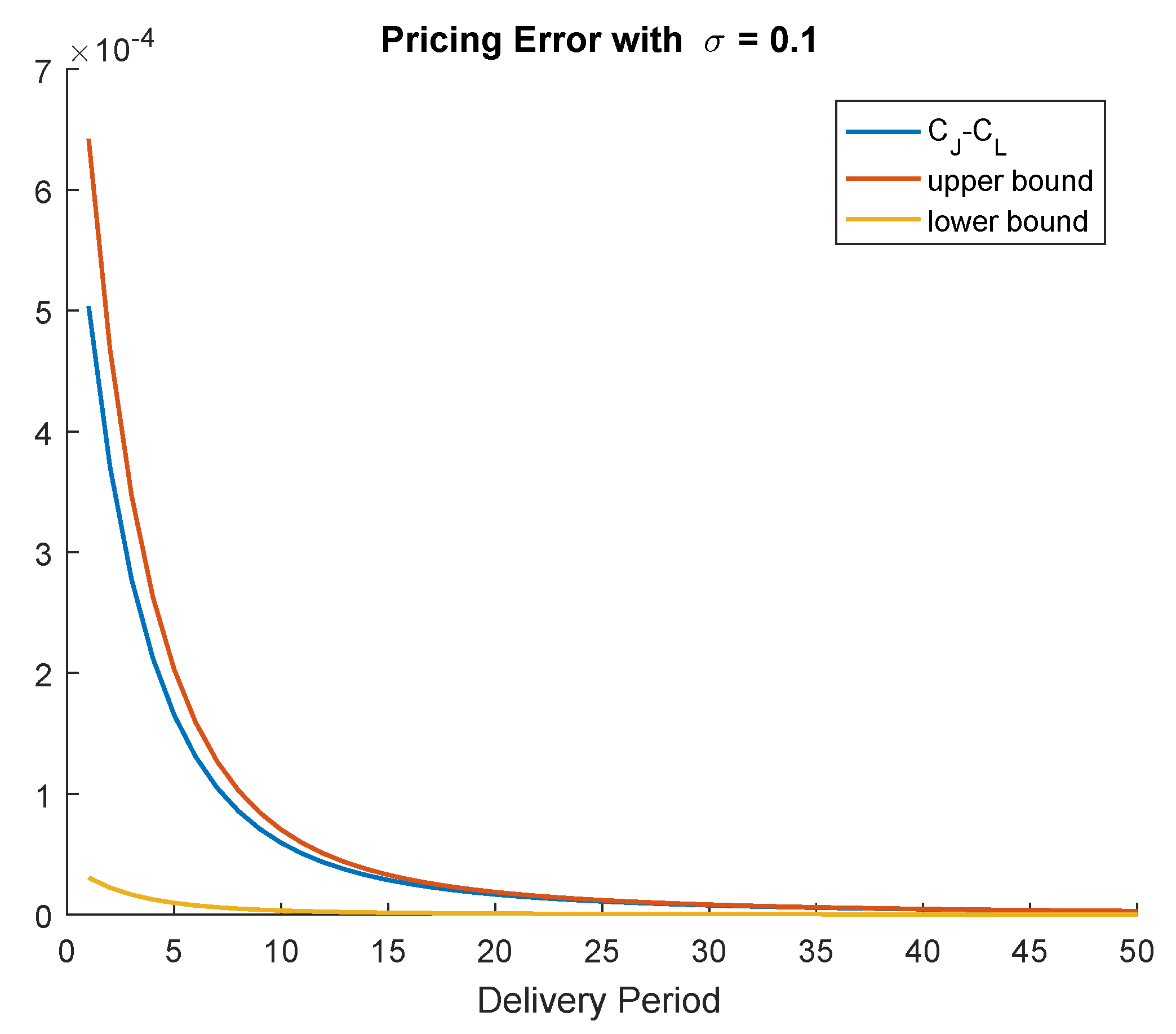
The parameters are all constant, and given by , , for all . The values of and are chosen as in Schmeck (2016); that is, is the fast mean-reversion rate, while is the slower one. We consider options at the money, that is . Finally, we set , for simplicity, the maturity of the option is , and the delivery period starts four days later (see Options Trading at EEX 2018). Figure 2 shows the pricing error that is made by using the above parameters. As our theoretical analysis proved, the error vanishes for long delivery periods. Here, we can see that the upper bound better fits the actual pricing error. However, the lower bound is quite far away from the actual error.
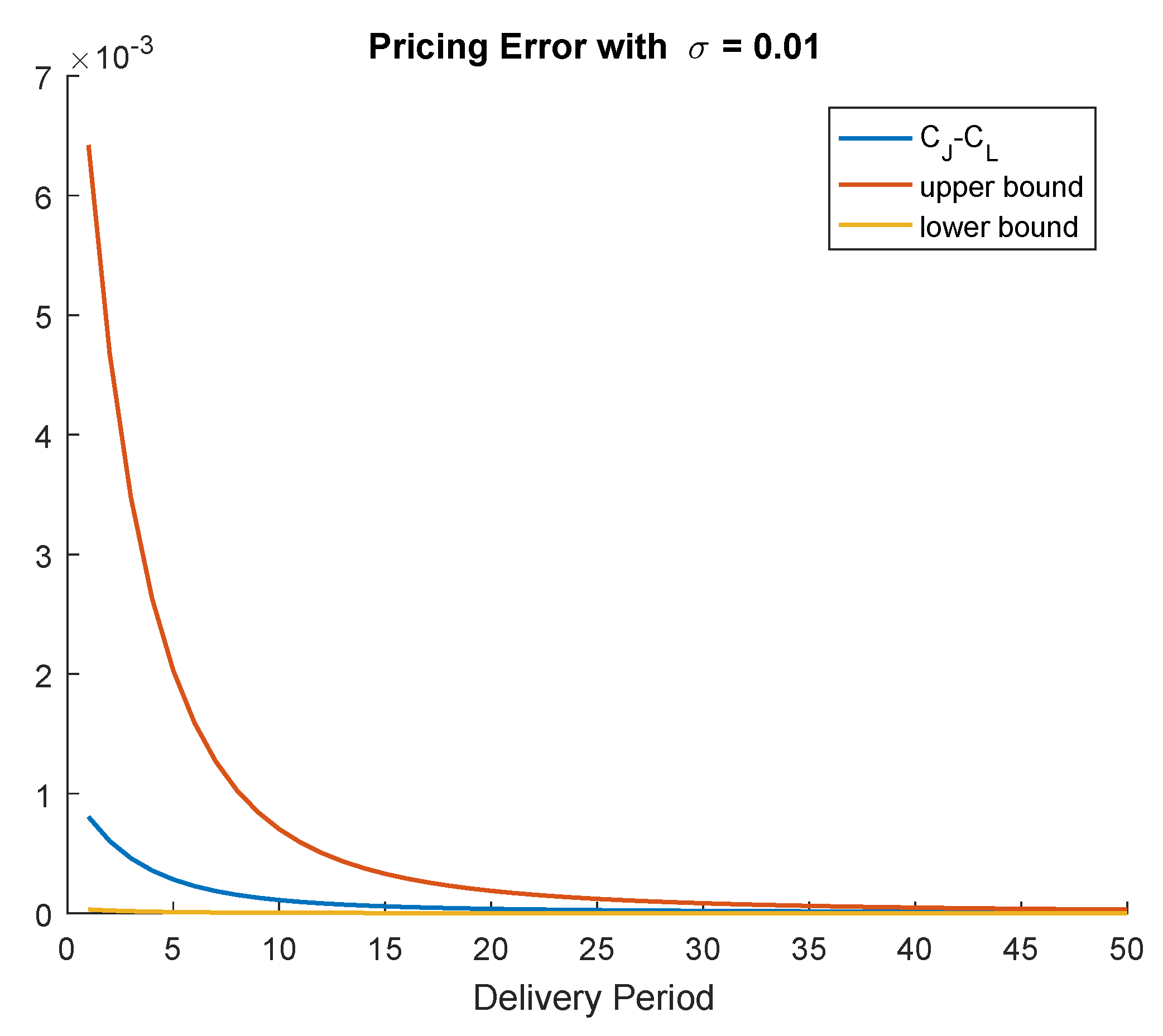
On the other hand, if we reduce to the value , we observe from Figure 3 that the situation reverse; i.e., the lower bound on the pricing error becomes closer to the actual difference than the upper bound. Overall, these numerical exercises illustrate that, depending on the model’s parameters, either the upper or the lower bound deliver better information about the real difference between the call options’ prices.
6. Conclusions
It is well known that price series in electricity markets exhibit several features such as jumps and multi-scale mean reversion. On one hand, multi-factor models can incorporate these stylized facts into a theoretical model framework. On the other hand, the more factors the more complex becomes estimation or calibration of the model to data. Not only the number of parameters increases, it is also not obvious to decide, e.g., what movements are due to a jump component, and what movements are best described to originate from a Brownian component. Therefore it is important to explore the role of the single factors when it comes to pricing of derivatives. In this paper, we have determined upper and lower error bounds for option prices when neglecting some factors of the original model. We place ourselves into an arithmetic setting, having the advantage of the possibility to include the delivery period explicitly. This is the main difference to the connected articles Benth and Schmeck (2014) and Schmeck (2016), that work in a geometric setting, and thus have to approximate the delivery period. Indeed, the length of the delivery period plays a crucial role, the longer the period the smaller the error when neglecting mean-reverting components. We illustrate our findings numerically and find that already for monthly delivery periods, the error one makes is typically very small, when neglecting fast mean reverting factors. Furthermore, the volatility of the non-stationary factor influences the quality of the error bounds. For small values, the pricing error is closer to the lower bound, while for higher values the upper error bound turns out to be more precise. Thus, for recently traded shorter delivery periods, e.g., on a weekly base, the error can be substantial, especially for smaller base volatility.
Author Contributions
Conceptualization, M.D.S. and S.S.; methodology, M.D.S. and S.S.; software, S.S.; formal analysis, M.D.S. and S.S.; writing—original draft preparation, M.D.S. and S.S.; writing—review and editing, M.D.S.; visualization, S.S.; supervision, M.D.S.; All authors have read and agreed to the published version of the manuscript.
Funding
This research received no external funding.
Institutional Review Board Statement
Not applicable.
Informed Consent Statement
Not applicable.
Data Availability Statement
Not applicable.
Acknowledgments
The authors thank Tiziano Vargiolu for suggesting to consider an arithmetic framework for the evaluation of the pricing error.
Conflicts of Interest
The authors declare no conflict of interest.
Appendix A
Appendix A.1. Proof of Theorem 1
Proof.
Plugging
into Equation (A1), noticing that is deterministic, that and are -measurable, and that the stochastic integrals are independent of , we obtain from Equation (A1)
Here, we have also employed Fubini’s theorem, whose use is justified by the fact that , and are bounded, and , by assumption.
Because the expectations of the Brownian stochastic integrals clearly vanish, by simple computations we obtain
Finally, we conclude by using that
□
Appendix A.2. Proof of Theorem 2
References
- Al-Sunaidy, Ali M. A., and Richard Green. 2006. Electricity deregulation in OECD (Organization for Economic Cooperation and Development) countries. Energy 31: 769–87. [Google Scholar] [CrossRef]
- Ball, Clifford A., and Walter N. Torous. 1983. A Simplified Jump Process for Common Stock Returns. The Journal of Financial and Quantitative Analysis 18: 53–65. [Google Scholar] [CrossRef]
- Benth, Fred E., and Maren D. Schmeck. 2014. Pricing and hedging options in energy markets using Black-76. Journal Energy Markets 7: 35–70. [Google Scholar] [CrossRef]
- Benth, Fred E., Jan Kallsen, and Thilo Meyer-Brandis. 2007. A Non-Gaussian Ornstein–Uhlenbeck process for electricity spot price modeling and derivatives pricing. Applied Mathematical Finance 14: 153–69. [Google Scholar] [CrossRef]
- Benth, Fred E., Jūratė Šaltytė Benth, and Steen Koekebakker. 2008. Stochastic Modeling of Electricity and Related Markets. Singapore: World Scientific. [Google Scholar]
- Benth, Fred E., Marco Piccirilli, and Tiziano Vargiolu. 2019. Mean-reverting additive energy forward curves in a Heath-Jarrow-Morton framework. Mathematics and Financisl Econonics 13: 543–77. [Google Scholar] [CrossRef]
- Borovkova, Svetlana, and Maren D. Schmeck. 2017. Electricity price modeling with stochastic time change. Energy Economics 63: 51–65. [Google Scholar] [CrossRef]
- Deschatre, Thomas, Olivier Féron, and Pierre Gruet. 2021. A survey of electricity spot and futures price models for risk management applications. arXiv arXiv:2103.16918. [Google Scholar]
- Edoli, Enrico, Marco Gallana, and Tiziano Vargiolu. 2017. Optimal intra-day power trading with a Gaussian additive process. Journal Energy Markets 10: 23–42. [Google Scholar]
- Escribano, Alvaro, Juan Ignacio Pena, and Pablo Villaplana. 2011. Modeling electricity prices: International evidence. Oxford Bulletin Economics Statistics 73: 622–50. [Google Scholar] [CrossRef] [Green Version]
- Fanelli, Viviana, and Maren D. Schmeck. 2019. On the seasonality in the implied volatility of electricity options. Quantitative Finance 19: 1321–37. [Google Scholar] [CrossRef]
- Fanone, Enzo, Andrea Gamba, and Marcel Prokopczuk. 2013. The case of negative day-ahead electricity prices. Energy Economics 35: 22–34. [Google Scholar] [CrossRef]
- Geman, Helyette, and Andrea Roncoroni. 2006. Understanding the fine structure of electricity prices. Journal Business 79: 1225–61. [Google Scholar] [CrossRef] [Green Version]
- Genoese, Fabio, Massimo Genoese, and Martin Wietschel. 2010. Occurrence of negative prices on the German spot market for electricity and their influence on balancing power markets. Paper presented at 2010 7th International Conference on the European Energy Market, Madrid, Spain, June 23–25; pp. 1–6. [Google Scholar]
- Hinderks, Wieger J., and Andreas Wagner. 2020. Factor models in the German electricity market: Stylized facts, seasonality, and calibration. Energy Economics 85: 104351. [Google Scholar] [CrossRef]
- Kaminski, Vincent. 2013. Energy Markets. London: Risk Books. [Google Scholar]
- Kiesel, Rüdiger, Gero Schindlmayr, and Reik H. Börger. 2009. A two-factor model for the electricity forward market. Quantitative Finance 9: 279–87. [Google Scholar] [CrossRef]
- Knittel, Christopher R., and Michael R. Roberts. 2001. An Empirical Examination of Deregulated Electricity Prices. Boston: Boston University. [Google Scholar]
- Latini, Luca, Marco Piccirilli, and Tiziano Vargiolu. 2019. Mean-reverting no-arbitrage additive models for forward curves in energy markets. Energy Economics 79: 157–70. [Google Scholar] [CrossRef]
- Meyer-Brandis, Thilo, and Peter Tankov. 2008. Multi-factor jump-diffusion models of electricity prices. International Journal of Theortical and Applied Finance 11: 503–28. [Google Scholar] [CrossRef] [Green Version]
- Musiela, Marek, and Marek Rutkowski. 1997. Martingale Methods in Financial Modelling. Berlin: Springer. [Google Scholar]
- Nomikos, Nikos K., and Orestes A. Soldatos. 2010. Analysis of model implied volatility for jump diffusion models: Empirical evidence from the Nordpool market. Energy Economics 32: 302–12. [Google Scholar] [CrossRef]
- Options Trading at EEX. 2018. Available online: https://www.eex.com/blob/57714/b2b2e9d0dfd4b2895735f3ff8e53b915/20160914-eex-presentation-milan-event-1-data.pdf (accessed on 29 January 2018).
- Piccirilli, Marco, Maren D. Schmeck, and Tiziano Vargiolu. 2021. Capturing the power options smile by an additive two-factor model for overlapping futures prices. Energy Economics 95: 105006. [Google Scholar] [CrossRef]
- Schmeck, Maren D. 2016. Pricing Options on Forwards in Energy Markets: The Role of Mean Reversion’s Speed. International Journal of Theortical and Applied Finance 19: 1650053. [Google Scholar] [CrossRef] [Green Version]
- Weron, Rafal. 2014. Electricity price forecasting: A review of the state-of-the-art with a look into the future. International Journal of Forecasting 30: 1030–81. [Google Scholar] [CrossRef] [Green Version]
Figure 1.
A sample path of , (upper), and of S (lower). The jumps’ sizes of the s are normally distributed with zero mean and variance 2, while the jumps’ frequency is set . As for the plot of S, we have taken , and, with regards to X, and .
Figure 1.
A sample path of , (upper), and of S (lower). The jumps’ sizes of the s are normally distributed with zero mean and variance 2, while the jumps’ frequency is set . As for the plot of S, we have taken , and, with regards to X, and .

Figure 2.
The pricing error with and without jumps.

Figure 3.
The pricing error with and without jumps.

Publisher’s Note: MDPI stays neutral with regard to jurisdictional claims in published maps and institutional affiliations. |
© 2021 by the authors. Licensee MDPI, Basel, Switzerland. This article is an open access article distributed under the terms and conditions of the Creative Commons Attribution (CC BY) license (https://creativecommons.org/licenses/by/4.0/).
Share and Cite
MDPI and ACS Style
Schmeck, M.D.; Schwerin, S. The Effect of Mean-Reverting Processes in the Pricing of Options in the Energy Market: An Arithmetic Approach. Risks 2021, 9, 100. https://doi.org/10.3390/risks9050100
AMA Style
Schmeck MD, Schwerin S. The Effect of Mean-Reverting Processes in the Pricing of Options in the Energy Market: An Arithmetic Approach. Risks. 2021; 9(5):100. https://doi.org/10.3390/risks9050100
Chicago/Turabian StyleSchmeck, Maren Diane, and Stefan Schwerin. 2021. "The Effect of Mean-Reverting Processes in the Pricing of Options in the Energy Market: An Arithmetic Approach" Risks 9, no. 5: 100. https://doi.org/10.3390/risks9050100
Note that from the first issue of 2016, this journal uses article numbers instead of page numbers. See further details here.