
A Finite Mixture Modelling Perspective for Combining Experts’ Opinions with an Application to Quantile-Based Risk Measures


Department of Statistics, London School of Economics and Political Science, London WC2A 2AE, UK
*
Authors to whom correspondence should be addressed.
Risks 2021, 9(6), 115; https://doi.org/10.3390/risks9060115
Submission received: 27 April 2021
/
Revised: 28 May 2021
/
Accepted: 2 June 2021
/
Published: 9 June 2021
(This article belongs to the Special Issue Risks: Feature Papers 2021)
Abstract
:The key purpose of this paper is to present an alternative viewpoint for combining expert opinions based on finite mixture models. Moreover, we consider that the components of the mixture are not necessarily assumed to be from the same parametric family. This approach can enable the agent to make informed decisions about the uncertain quantity of interest in a flexible manner that accounts for multiple sources of heterogeneity involved in the opinions expressed by the experts in terms of the parametric family, the parameters of each component density, and also the mixing weights. Finally, the proposed models are employed for numerically computing quantile-based risk measures in a collective decision-making context.
1. Introduction
“Opinion is the medium between knowledge and ignorance” is an expression that is ascribed to Plato. Indeed, due to the growing uncertainty in an abundance of contemporary societal settings, we often come across circumstances when an agent, who acts on behalf of another party, is called to make a decision by combining multiple and sometimes diverging sources of information that can be described as opinions. Moreover, the latter may take any form; from experts to forecasting methods or models (see Clemen and Winkler (2007)), and from now on, we may use these terms interchangeably when referring to an opinion. Opinions communicated to an agent can differ to varying degrees, and the level of confidence that an agent allocates to any given viewpoint is subjective.
Some examples where an idiosyncratic combination of opinions is required for a decision to be made at an individual, corporate, and policy level follow. In the private sphere, consider an individual who plans to sell their house, and in doing so consults property experts to determine an appropriate selling price. While the latter may be influenced by some "standard" factors, such as the number of bedrooms in a given postcode, various experts may additionally examine different price determinants such as the proximity of the property to a good school or a park. That said, the seller may want to incorporate all this diverse information in an effort to achieve a better financial outcome for themselves, but the weight that each reported opinion has in this process lies mostly on the seller’s perception. In a financial corporate environment, consider the case where an investment manager asks a number of quantitative analysts to evaluate the return on a stock. Disagreement in opinions here could arise from the fact that some analysts may be more optimistic than others about the future. As mentioned in Peiro (1999), aggregate stock market returns are asymmetrically distributed; the largest movements in the market usually refer to decreases rather than increases in returns. As a result, one can say that an analyst foreseeing a regime shift, let us say, close to a firm’s earnings announcement period (see McNichols (1988)) would possibly choose a more heavy-tailed distribution to model the returns compared to others who did not have such a negative expectation. Once again, an investment manager decides on the level of trust to show to any given opinion, based on their own subjective criteria. Finally, at a public policy level and in light of the COVID-19 pandemic, policy makers consult experts from a variety of disciplines, such as anthropology, mathematics, statistics, epidemiology, and engineering, to name a few (see Government Office for Science (2020)) to enable them to build the strategy for its effective management. Reported opinions may not always align, as each specialist sees the problem from a different angle. Government officials though, regardless of divergent opinions, need to combine and evaluate the weight of each view for policy decisions. The subjective character of how much emphasis is given to each opinion by a given policy maker is apparent by the recorded observations of so many different responses related to handling the pandemic across different countries. Similarly to the aforementioned quandaries, decision dilemmas have long been investigated in the particularly rich literature concerning combinations of opinions, which, as Clemen and Winkler (1999) indicate, embraces a number of behavioural and quantitative approaches. See Section 2 for a detailed literature review.
Let us now discuss our motivation behind this study. As is well known, in quantitative risk management, the process of defining, measuring and managing operational risk is crucial since it formalizes the financial institutions’ approaches to comply with the qualifying qualitative criteria of the Basel Capital Accord and Solvency Directive. This approach relies on the knowledge of experienced enterprise agents and risk management experts who are asked to provide opinions regarding plausible high-severity events. For instance, these opinions can be expressed as parameters of an assumed loss distribution. However, the company’s risk profile, which could accord to a consensus of experts’ individual judgements regarding the severity distribution, might often not be robustly estimated. The main reason for this is that when experts are presented with internal data and need to express probabilistic opinions about the same uncertain quantity of interest, there may be multiple sources of heterogeneity in their responses concerning the choice of models and their parameters and, in addition to these, the allocation of weights from the agent that are not considered as being embedded in the data-generative process of the uncertain quantity of interest based on which the agent needs to make a decision. In particular, each expert reports their opinion based on what their focus is, and if we assume that they report their opinions honestly, each believes that their opinion reflects best the true data-generative process. Therefore, since a major challenge in operational risk management is to evaluate the exposure of severe losses based on a weighted combination of a variety of opinions in the first place, it appears that it would make more sense to employ probabilistic models that reflect group structures.
In this paper, we present an alternative perspective for modelling of operational risk in an enterprise context by combining expert opinions based on finite mixture models. Finite mixtures models can provide a formal framework for clustering and classification that can be effectively used within the opinions combination research setting. In particular, this versatile and easily extensible class of models can accommodate different sources of unobserved heterogeneity in the data-generative process of the uncertain quantity of interest by allowing for the mixture components to represent groups within which there is a concurrence of judgements. At this point, it is worth noting that finite mixtures models have not been applied in the area of opinion combinations, with the exception of Rufo et al. (2010), who employed Bayesian hierarchical models based on mixtures of conjugate prior distributions for merging expert opinions. Furthermore, it should be noted that Shevchenko and Wüthrich (2006) employed the Bayesian inference method for quantifying frequency and severity distributions in the context of operational risk. Their approach was based on specifying the prior distributions for the parameters of the frequency and severity distributions based on expert opinions or external data. Furthermore, Lambrigger et al. (2009) extended the framework of the previous paper by developing a Bayesian inference model that permits combining internal data, external data, and expert opinions simultaneously. The setup they proposed enlarged the Bayesian inference models of the exponential dispersion family (EDF) and their corresponding conjugate priors; see, for instance, Bühlmann and Gisler (2006), Chapter 2. However, to the best of our knowledge, the use of finite mixture models within the traditional frequentist approach for combining diverging opinions remains a largely uncharted research territory. Our main contribution is that we consider that the component distributions can stem from different parametric families. The advantage of this formulation is that it allows the agent to obtain the aggregated opinion of a group of experts, based on a linear opinion pool, and account for the various sources of unobserved heterogeneity in the decision-making process in the following ways: (i) by assuming that the data are drawn from a finite mixture distribution with components representing different opinions about both the distribution family and its parameters regarding the uncertain quantity of interest, and (ii) via the mixing weights that reflect the quality of each opinion. Furthermore, when the proposed family of models is applied to internal data, it can enable the agent to utilize all the available information for accurately assessing the effectiveness of (i) the combination of the expert judgements and (ii) their own judgement about the weights that they intended to allocate to each expert—a concept not so dissimilar to the the main idea behind the long-established weights allocation approach of Cooke (1991) and the scoring rules in general. Finally, the proposed family of models is used for numerically computing quantile-based risk measures, which are of interest in a variety of different types of insurance problems, such as setting premiums, insurance deductibles, and reinsurance credance levels and determining reserves or capital and ruin probabilities.
The rest of this paper proceeds as follows. Section 2 provides a brief literature review on some traditional approaches for combining diverging opinions. Section 3 explores the topic of combining diverging opinions using finite mixture models. Section 4 describes the calculation of quantile-based risk measures based on the finite mixture modelling methodology. In our numerical application, we focus on quantile-based risk measures. Finally, concluding remarks can be found in Section 5.
2. Traditional Approaches for Combining Expert Judgements
In this section, we briefly present some famous approaches in aggregating expert judgements. The latter topic can be seen from different perspectives, and in recent decades, several quantitative and behavioural methods have been used for its study. That said, no method can be considered superior to another because for each opinion combination problem, a whole process should be established to identify the most appropriate combination strategy; see Clemen and Winkler (1999). In doing so, factors such as experts’ availability, degree of divergence in opinions, past experience regarding the experts, and the random quantity of interest among others should all be considered. As one would expect, such diversity in approaches to combining judgements has resulted in a rich and interdisciplinary literature that would be impossible to cover in its entirety in this article; however, we provide a short review of some important works.
2.1. Behavioural Approaches
Behavioural approaches to opinion aggregation typically involve sources of information, commonly referred to as experts, interacting with each other in order to reach some conclusions. This interaction between experts can happen in a direct or indirect manner. For instance, in an approach called feedback and re-assessment (see Winkler (1968)) no direct communication is allowed among the experts. The agent first collects the views of each individual expert, and then each of them is presented with the other expert opinions and given the opportunity to revise their own view and re-submit it to the agent. Multiple rounds of this process may be required to reach a consensus, or at least to decrease the number of diverging views, thus simplifying decision making. Subsequently, these views may need to be quantitatively combined. One of the earliest methods associated with the feedback and re-assessment approach is known as the Delphi Method; see Linstone and Turoff (1975); Dalkey (1969), and Parenté and Anderson-Parenté (1987).
Additionally, another behavioural aggregation approach, which is known as group re-assessment (Winkler (1968)), allows for direct discussion between experts, after they have individually shared their view, in search of a group opinion consensus. Examples of methods falling into this category are the Nominal Group technique and Kaplan’s approach; see Delbecq et al. (1975) and Kaplan (1992), respectively. An advantage of such group reassessment approaches is that experts, when given the opportunity to discuss, may find that there are other factors to consider that would have been otherwise overlooked. However, the fact that the experts need to make a decision as a group comes with certain complications, which we discuss briefly below.
In particular, if we assume that the initial individual opinions are expressed in terms of probability distributions, the moment that discussion between experts starts, each expert also brings considerations about their individual utility function. Furthermore, psychological factors have a role to play in reaching common agreement; some experts may have more advanced leadership skills than others, which may result in the latter adjusting their views merely to reach consensus without necessarily agreeing on the outcome. Last but not least, a phenomenon called polarisation may happen when the group takes riskier decisions as a whole compared to if an individual were to make a decision alone; see Plous (1993) and Wallach et al. (1962). However, this is certainly not to say that the choice to use group decisions is flawed; direct group interactions can be functional in certain circumstances; see Hogarth (1977). Having discussed some behavioural methods, we continue with the presentation of a few quantitative approaches for combining diverging expert opinions.
2.2. Quantitative Approaches
Addressing the problem of combining opinions quantitatively often involves analytical models and procedures operating on individual probability distributions to yield a single combined distribution; see Winkler (1968); French (1983); Genest (1992); Cooke (1991); Clemen (1989), and Clemen and Winkler (1999) for an overview. Focusing on the field of quantitative combination of probability distributions, we see that the linear, logarithmic, and Bayesian pooling methods are typical approaches—a summary of the general ideas behind these methods follows.
The linear pool (see Stone (1961)) and logarithmic pool (see Genest et al. (1984) and Clemen and Winkler (1999)) involve, respectively, a weighted linear or multiplicative combination of the expert probabilities. Out of the two, the linear pool is often perceived as a more attractive combination method because of its intuitiveness and the fact that it satisfies a number of convenient properties; see Cooke (1991) and Clemen and Winkler (1999). In the Bayesian framework, the agent firstly determines a prior distribution over the values of the examined random variable, and then information provided by other sources, say experts, is merely seen as observed data. These “data” are then inserted into a likelihood function along with the prior distribution of the agent to derive a posterior distribution. Although interesting, the implementation of this approach can be challenging in practice; see Bolger and Houlding (2016).
Furthermore, an important note is the meaning of the word “probabilities” in the quantitative opinion combination literature. Whilst traditionally, “probabilities” means mass or density functions for the discrete case and continuous case, respectively Clemen (1989), in recent years, there has been some evidence that combining quantiles, first suggested by Vincent (1912), might be at least as good as combining probability densities (see Lichtendahl et al. (2013); Busetti (2017); Bansal and Palley (2017); Hora et al. (2013); Bogner et al. (2017), and Jose et al. (2013)), despite some criticism from Colson and Cooke (2017). Quantiles combination was also found to be preferable when individual forecasts are biased; see Bamber et al. (2016) and Lichtendahl et al. (2013). Next, we discuss the topic of weights allocation, which, as we will see, is once again a subjective matter depending on the opinions combination problem in question.
2.3. Weights Determination
When combining competing views, the determination of weights is difficult because there are no methods for weights allocation obtained straight from first principles; see Clemen (2008). Nevertheless, the interpretation of weights is flexible, and as Genest and McConway (1990) mention, based on the meaning chosen, one can direct oneself in selecting an appropriate method for their computation. Generally speaking, the weights should somehow reflect the quality of expert opinions; see Bolger and Houlding (2016). When weights are interpreted in this way, the evaluation of the quality of probabilistic forecasts entails the computation of performance measures that account for what has happened in reality; see Winkler et al. (1996) and Gneiting and Raftery (2007).
Such measures, known as scoring rules, play an ex post and ex ante role in the evaluation of probabilities reported; see Winkler et al. (1996): an ex post role because the decision maker needs to first observe what happens in reality before they can truly assess the quality of probabilities experts have reported, and an ex ante role because the experts anticipate the ex post evaluation from the agent and thus have an incentive to be honest when they are expressing their opinions. There are many scoring rules, even though the most preferred are those called strictly proper, meaning that an expert can only maximise their score for an expressed opinion by reporting their forecast honestly; see Winkler et al. (1996) and Gneiting and Raftery (2007). Overall, the choice of scoring rule would in turn lead to different weights; see Genest and McConway (1990).
That said, probably one of the most famous approaches for weights determination, often referred to as the "classical" method, is the one presented in Cooke (1991). There, before making a decision, the agent requests experts to provide their views on quantities whose values are known to the agent but totally unknown to the experts. See Cooke and Goossens (2008) and Eggstaff et al. (2014b) for merits of the "classical" approach, Eggstaff et al. (2014a) for a novel way to make it account for sequential weight updating, and Flandoli et al. (2011) for shortcomings and some alternatives to the "classical" approach. Given the complication involved in weights calculation, the simple averaging scheme is popular in practice because of its perceived robustness and simplicity (see O’Hagan et al. (2006); Lichtendahl et al. (2013)), whilst there is no clear indication that it performs worse than Cooke’s approach; see Clemen (2008).
All in all, it should be mentioned that there is limited literature on determining the opinion weights, but for the interested reader, the recent work of Koksalmis and Kabak (2019) provides a comprehensive literature review across various disciplines, suggesting a classification system with the following categories: similarity-based approaches, index-based approaches, clustering-based approaches, integrated approaches, and other approaches. Moving forward to Section 3, we recommend an alternative approach in the area of quantitative combination of probabilistic opinions based on finite mixture models. Such an approach has the benefit of accounting for various forms of heterogeneity among expert views, and straightforward weights computation being able to deal with even a large number of experts.
3. A Finite Mixture Modelling Viewpoint for Opinions Combination
In this section, we present a different approach and incorporate finite mixture models into the diverse set of methodologies for aggregating different opinions. We start by explaining the motivation behind our proposal, followed by a formal presentation of finite mixture models. We then explain how the finite mixture model framework is interpreted for the purposes of combining judgements.
3.1. Motivation Behind the Suggested Approach
Thinking about opinions in the context of distributions or models, in the traditional framework of combining judgements, described in Section 2, each expert gives the agent a different model, and then these individual models are combined into a single model with weights being decided by the agent—most often by taking the weighted average of the individual probability density functions or quantiles. Our proposed finite mixture modelling perspective provides a platform for opinion pooling in two stages. Firstly, we cluster expert opinions of the same kind, and secondly, we perform a convex combination of different clusters using mixing weights that represent the quality of each opinion as this is perceived by the agent. Using historical data, the maximum likelihood (ML) estimation of the parameters and weights can reveal whether both parties are rigorous in their judgements.
3.2. Finite Mixture Models
We start by giving some background on finite mixture models and their use across multiple disciplines and then provide their mathematical definition.
3.2.1. Overview
Finite mixtures is a flexible and easily extensible class of models that account for unobserved heterogeneity; see, for instance, Newcomb (1886); Pearson (1894); Everitt and Hand (1981); Titterington et al. (1985) and McLachlan and Basford (1988) and McLachlan et al. (2019). In particular, starting from a sample of observations, which are assumed to come from a number of underlying classes with unknown proportions, the density of the observations in each of these classes is determined for the purpose of decomposing the sample into its mixture components; see Wedel and DeSarbo (1994). It should be noted that the popularity of mixture models has spread substantially in works of applied and methodological interest across various disciplines such as insurance, economics, finance, biology, genetics, medicine, and most recently in the sphere of artificial intelligence. A few notable works across the aforementioned disciplines include these of Titterington (1990); Samadani (1995); Yung (1997); Allison et al. (2002); Karlis and Xekalaki (2005); McLachlan et al. (2005); Grün and Leisch (2008); Efron (2008); Schlattmann (2009); Bouguila (2010); Mengersen et al. (2011); Elguebaly and Bouguila (2014); Tzougas et al. (2018); Henry et al. (2014); Miljkovic and Grün (2016); Gambacciani and Paolella (2017); Oboh and Bouguila (2017); Tzougas et al. (2014); Miljkovic and Grün (2016); Punzo et al. (2018); Blostein and Miljkovic (2019); Chai Fung et al. (2019); Caravagna et al. (2020), and Bermúdez et al. (2020), though this list is certainly not exhaustive. A short summary of the main characteristics of the class of finite mixture models with component distributions stemming from different parametric families, which we consider in this study follows. The interested reader can also refer to McLachlan and Peel (2000b) for a more detailed treatment of finite mixture models and to McLachlan et al. (2019) for an up-to-date account of the theory and methodological developments underlying their applications.
3.2.2. Definition
Consider that is a sample of independent and identically distributed (i.i.d.) random variables from an n-component finite mixture distribution with density function
where , with , where denotes the parameters of the density function , and where is the vector of component weights, with the prior (or mixing) probability of the component z, where and holds. Furthermore, assume that the density functions are absolutely continuous with respect to the Lebesgue measure and are elements from univariate parametric families with a d-dimensional parameter vector , , .
At this point, it is worth noting that, under the proposed modelling framework, the component distributions in Equation (1) do not necessarily arise from the same parametric family. Therefore, our general approach allows for the design of more flexible models to include a large number of alternative convex combinations of heavy-tailed and light-tailed distributions. Moreover, with this formulation, this class of models can take into account heterogeneity in the data arising from three different sources, differing parameters, differing parametric families, and mixing weights.
3.2.3. Estimation via the Expectation Maximisation Algorithm
Consider the finite mixture model with the associated log-likelihood
where is given by Equation (1). The direct maximization of the above function with respect to the vector of parameters , is complicated. Fortunately, such a task can be easily achieved via the Expectation Maximization (EM) algorithm, which is the standard iterative method that is used for finding ML estimates for models with latent variables; see Dempster et al. (1977). In particular, the popularity of EM algorithm for fitting mixture models to data is such that, as stated in McLachlan et al. (2019), all research works on this topic after 1977 use this method because it unifies the ML estimation from data that can be viewed as being incomplete. For more details regarding the EM algorithm, the interested reader can, for instance, refer to the works of Titterington et al. (1985); McLachlan and Basford (1988); Couvreur (1997), and Karlis and Xekalaki (1999).
Regarding the implementation of the EM algorithm for ML estimation in the context of finite mixture models, we follow the standard approach of combining the observed data, which are represented by the random variable , with the set of unobserved latent random variables , where if the i-th observation belongs to the z-th component, and 0 otherwise, for and .
Then, the complete data log-likelihood of the model is given by
In what follows, at the E-Step of the algorithm, it is necessary to compute the Q-function, which is the conditional expectation of the complete data log-likelihood given by Equation (2), while the M-Step consists of maximizing the Q-function with respect to . A generic algorithm is formally described in what follows.
Using the current estimates and at iteration , calculate the “membership weights”:
for and . Note that is the posterior probability that comes from the mixture component z, calculated at the iteration of the EM algorithm. Thus, the Q-function is given by
Obtain new estimates for and by maximizing the Q-function:
- The updated estimates are given by:
- The updated estimates are obtained using a weighted likelihood approach for each of the different component distributions with weights given by Equation (3). It is clear that ML estimation can be accomplished relatively easily when the M-Step is in closed form. On the contrary, when this is not the case, numerical optimization methods are required for maximizing the the weighted likelihood.
3.3. Opinions Combination Problem in a Finite Mixture Model Setting
When considering the application of finite mixtures in the area of opinions combination, the framework described in Section 3.2 can be adjusted as follows. A decision maker, otherwise called an agent, needs to make a decision about an random quantity of interest. Since this decision is made under circumstances of uncertainty, the agent seeks for the opinion of an arbitrary number of consultants and the combined opinion is seen as a finite mixture model of the type described in 2.3.1 allowing for divergence in expert opinions, both in the class of and in components parameters . The mixing weights show the level of trust that the agent has to each expert. As in traditional approaches to expert opinions combination, the weights is up to the agent to determine. If the agent has access to older data about , the decision process can be made in two stages to ensure that weights allocation is right.
In the first stage, the agent fits alternative finite mixture models to the available internal data and identifies the mixing probabilities , the class of , and the parameters that lead to a robust estimation of the company’s risk profile. Then, the experts are asked to provide their views on class and given the old data without knowing that the agent knows the real answer. The agent checks the reply of the expert by comparing it to the correct answer, which, as mentioned previously, it is known to the agent but unknown to the expert. In the second stage, the agent needs to make a decision on a totally unknown situation and thus provides the data of real interest to Z experts. Assuming that past experts’ performance in getting a good answer indicates their future ability in providing reliable advice, the agent has an indication of how much trust should be given to the consultant. Assessing the quality of a probabilistic forecast on an ex post and ex ante basis using real data is not much different from the rationale of using scoring rules as mentioned in Section 2.1. In what follows, we present an application of finite mixture models to combine expert views in a financial setting and in particular when multiple experts are given the task to compute the financial risk measure Value at Risk ().
4. Application to a Quantile-Based Financial Risk Measures Setting
In this section, we apply a finite mixture methodology to address the issue of combining diverging expert opinions in an insurance context. We assume that the experts are actuaries and that the opinions expressed by each of them refer to the reserve, or otherwise risk measure, that the institution needs to report to the financial regulator. In particular, without loss of generality, we focus on the popular risk measure called Value at Risk () having the quantile as core ingredient; however our general approach can be applied to any quantile-based risk measure. Any discussion from now on is focused on quantiles because, as we will later on see, the latter is the core ingredient of . We start by giving a brief presentation of risk measures and using a general notation, and then the application using simulated finite mixture data follows.
4.1. Motivation Behind the Application
Financial institutions are subject to a number of economic capital requirements following Basel II and Basel III directives in the banking sector and Solvency II and the Swiss Solvency Test in the insurance industry. Since the regulators do not instruct the use of a specific model for the calculation of the reserve, otherwise called risk measure, the choice of any probabilistic model that is used internally by a financial institution for calculating risk measures is crucial.
The above-mentioned challenge known as model risk (see Barrieu and Scandolo (2015) and Barrieu and Ravanelli (2015), among others) is of paramount importance for the health of the financial system along with the choice of the risk measure itself by the regulator; see Danielsson et al. (2001) and Embrechts et al. (2014). The multiple model alternatives for computing a given risk measure can be seen through the prism of an opinions’ combination problem. A financial institution, being an agent, instructs actuaries to present alternative internal models for the computation of a risk measure such as . In presence of model risk, the agent prefers to use a combination method to take into account the different opinions, i.e., models, prior to reaching a capital reserve decision.
In the context of combining expert opinions for computing quantile-based risk measures, such as , there is a clear advantage that the suggested finite mixture modelling approach enjoys over the classical approach of calculating quantiles such as the weighted average of individual quantiles coming from the expert judgements; see, Lichtendahl et al. (2013). This is that it provides a way to assess if the information from the experts that determines the decision-making process of the agent and the data-generative process are highly “synchronous” under a single chosen model in order to ensure that the resulting risk measure value can, as accurately as possible, determine the minimum cushion of economic liquidity.
Finally, under our general approach, which allows for flexibility in the choice of the component distributions which reflect different expert opinions, the resulting risk measures can be calculated using a convex combination of an abundance of alternative heavy-tailed and light-tailed distributions. Thus, since risk measures are equal or proportional to solvency capital requirements, the adopted modelling framework allows us to strike the right balance between calculating risk measures that are not too conservative and hence are preferred by financial institutions and insurance companies who wish to minimise the level of their reserves, since there are many restrictions on how this money can be invested, and computing stricter risk measures that would rather be imposed by regulators who wish to protect consumers. Moving forward, we start by defining financial risk measures in general before narrowing down to Value at Risk, which we use in our application.
4.2. Risk Measures
Financial institutions want to know the minimum amount of capital to add to a position they take in the market to make it acceptable from a regulatory viewpoint. From now on, our random quantity of interest is a financial position. More precisely, a financial position is a mapping
where is an non-empty set representing a fixed set of possible scenarios. Let be a scenario that is part of . Then reflects the terminal value of the position (profit or loss) at the end of the trading period if the scenario ∈ is observed. Assuming that is a set of financial positions, we let the financial position belong to it. Whilst from an economic perspective would have to be of a very large size, preferably the space of all , it is quantitatively convenient to introduce the restriction of boundedness. Furthermore, is a linear space containing the constants. At this point, we do not fix a probability measure in .
To calculate the capital requirement, an actuary finds some number that quantifies the risk of taking the financial position . In particular, a monetary risk measure is a mapping
which satisfies the following conditions
The condition of monotonicity simply reflects the fact that a position yielding a higher payoff in all scenarios, i.e., in the whole , carries less risk. The cash invariance property demonstrates that risk is measured in monetary units, meaning when an amount m is added to a risky position, its risk will decrease by the same amount m. Normalisation implies that if one has nothing, there is no need to put aside any reserve.
There is a variety of risk measures (see, for instance Barrieu and El Karoui (2005); Föllmer and Schied (2010); Acciaio and Penner (2011); Föllmer and Schied (2016)), and in many cases, quantiles are a key ingredient. That said, for an , the -quantile of a random variable on a probability space , where is a probability measure on a measurable space , is any real number Q that satisfies the property
The set of all -quantiles of is an interval where the lower quantile function of is
and the upper quantile function of is
A very famous risk measure upon which the financial and insurance industry heavily relies is Value at Risk (). If we fix some level , the of a financial position at level is defined as
where is the upper quantile function of . The financial interpretation of is the smallest amount of capital, which, if added to the position and invested in a risk-free manner, ensures that the probability of a negative outcome is below the level . In the following subsection, we discuss how quantile-based risk measures, such as , can be numerically computed in the case of finite mixtures utilising the EM algorithm.
4.3. Computation of V@R Using Finite Mixtures Models
In the context of computing quantile-based risk measures using finite mixtures models, one should take into account that there is no closed-form solution and numerical estimation is required. For expository purposes, we present the numerical calculation of the using a finite mixture modelling methodology in the context of combining diverging expert opinions. However, note that the computation of other quantile risk measures, with many more interesting properties than the , such as the Tail Value at Risk () is straight forward using finite mixture models. For more details, one can refer to Miljkovic and Grün (2016). Since under the modelling framework we propose the component distributions can stem from different parametric families further interesting results can be obtained.
Let , presented in Section 3.2, be the random vector of financial positions of a financial institution introduced in Section 4.2. As we have seen in Section 4.2, is the -quantile of the distribution of financial position , and it satisfies the following property
Since in the context of finite mixture models, the does not have a closed-form solution, we compute it numerically by solving Equation (4)
where is the cumulative distribution function of the random financial position .
In particular, the numerical computation of can be achieved easily using the R programming language in a two-step process. Firstly, we create an R function according to Equation (1) with the only difference that now is replaced by as follows
where , where , and represents the vector of unknown parameters, is the prior (or mixing) probability of the component z where and holds. Secondly, we create the inverse function of denoted as , which is the . The function is derived in R by returning the argument in the package stats in R of () for a pre-determined quantile bracket. It should be mentioned that in order to evaluate at the point x, one needs to utilise the EM algorithm to estimate the parameters and mixing probabilities of . In the end, in order to calculate the quantile using the function , one just needs to insert as arguments the the percentile upon which will be calculated as well as the vectors of estimated parameters and mixing probabilities. In Section 4.4, we present our numerical application.
4.4. Numerical Application
In this subsection, a numerical example is presented to illustrate the proposed approach for combining expert opinions. In particular, without loss of generality, we assume that the experts can be classified into two groups within each of which there is a consensus of opinions. In this context, the components represent different expert opinions about the distribution family and its parameters, whilst the weights reflect the quality of each opinion as this may be assessed by the agent.
In what follows, we generate multiple samples from two-component mixtures of some classical distributions where the components of the mixture do not necessarily belong to the same parametric family. In particular, we consider the two-component (2C) Normal, 2C Gamma, 2C Lognormal, 2C Pareto mixtures, and also the 2C Lognormal-Gamma, and 2C Pareto-Gamma mixtures. Note that when using real data, one can distinguish between the competing models by employing the Deviance (DEV), Akaike information criterion (AIC), and the Schwartz Bayesian criterion (SBC). Furthermore, the prediction performances of the models can be assessed via out-of-sample validation. The prediction performances can be measured using the root-mean squared error (RMSE) and the deviance statistic. To provide a potential practical application of the proposed perspective, note that the convex combination of moderate and heavy-tailed distributions, similar to the aforementioned ones, can be used for efficiently approximating positive insurance loss data with right skewness, which can often be represented as an amalgamation of losses of different magnitudes. For example, Tzougas et al. (2014) and Miljkovic and Grün (2016) proposed the use of mixtures of finite mixture claim severity models in an actuarial setting, whilst Tzougas et al. (2018) and Blostein and Miljkovic (2019) considered finite mixture models where all components of the mixture are not necessarily assumed to be from the same parametric family.
The probability density functions (pdfs) of the component distributions, denoted by in Equation (1), are given by Equations (5)–(8) below.
- Normal distribution: the pdf of the Normal distribution is given by:for where and . The mean of is given by and the variance of X by . This parametric family is chosen for relatively symmetric insurance loss data, which take either positive or negative values.
- Lognormal distribution: the pdf of the Lognormal distribution is as follows:for where and . Here, and where .
- Gamma distribution: the density of the Gamma is given by:for , where and . This is a re-parameterisation, which was given in Equation (17.23) of Johnson et al. (1994) in p. 343, and it can be obtained by setting and . Moreover, and . The Gamma has a less heavier tail than the Lognormal one.
- Pareto distribution: the pdf of the Pareto distribution is as follows:for , where and . Furthermore, , and exists only if . This is an alternative distributional class choice that may be preferred to model more heavily right-skewed insurance loss data than the previous two distribution choices.
As described in Section 3.3, the fitting of such mixture distributions can be achieved via the EM algorithm, which is implemented for estimating both the parameters of each mixture component distribution and mixing weights. Subsequently, using these estimated values, we proceed with calculating the quantiles of the mixture models across all estimated weights combinations and for various probability levels (). At this point, it should be noted that we choose to compute quantiles directly from the finite mixture models, but for comparison purposes, we also combine quantiles for each expert view as it has often been encountered in the literature; see, for instance, Lichtendahl et al. (2013). Note also that the calculation of risk measures using finite mixture models has also been addressed by Miljkovic and Grün (2016) and Blostein and Miljkovic (2019). However, we would like to emphasise that this is the first time that the 2C Pareto and 2C Pareto-Gamma models are used for computing quantile based risk measures. Therefore, this constitutes one more novelty of our work in addition to proposing the finite mixture modelling approach as an efficient tool for combining expert opinions.
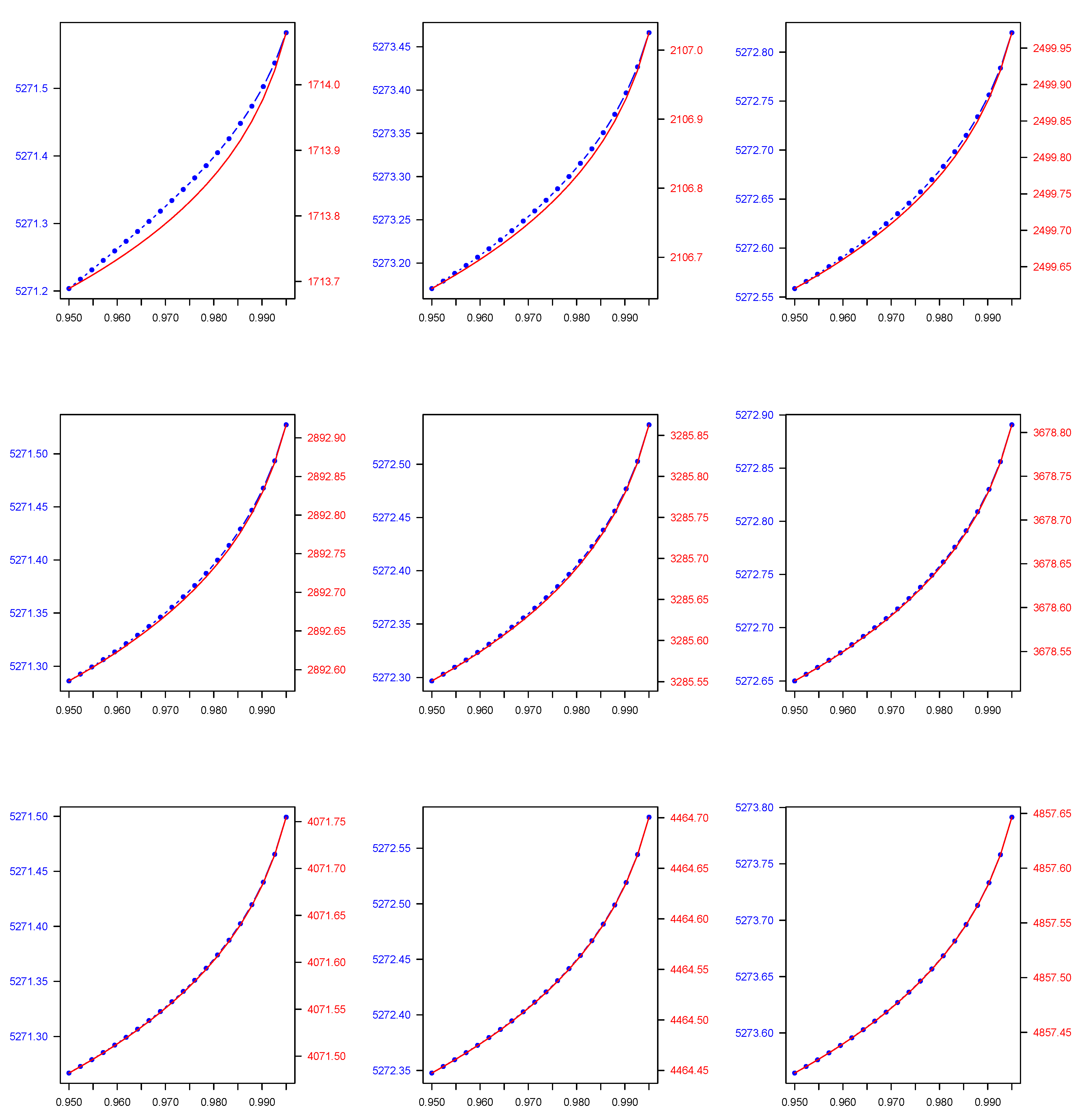
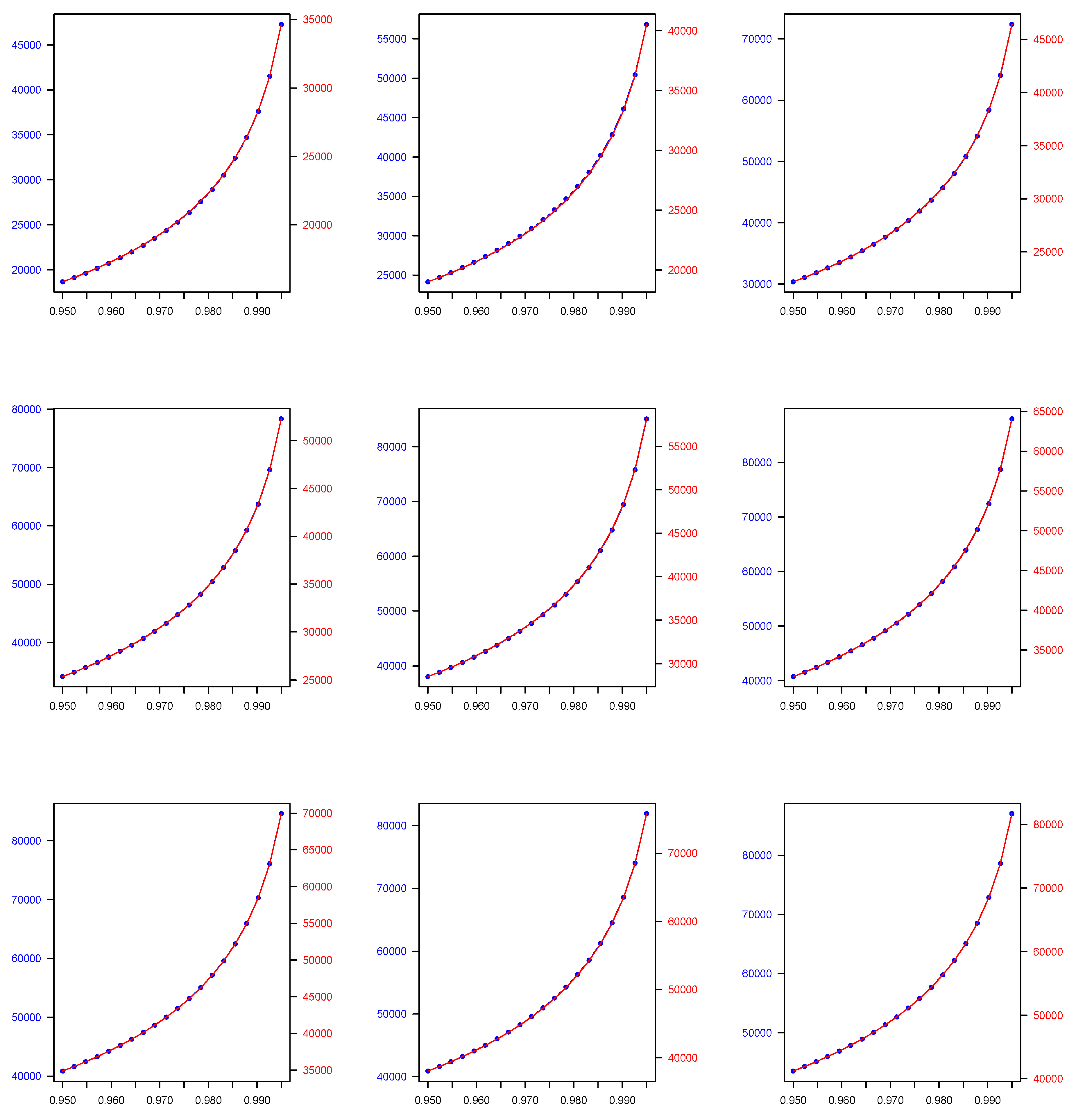
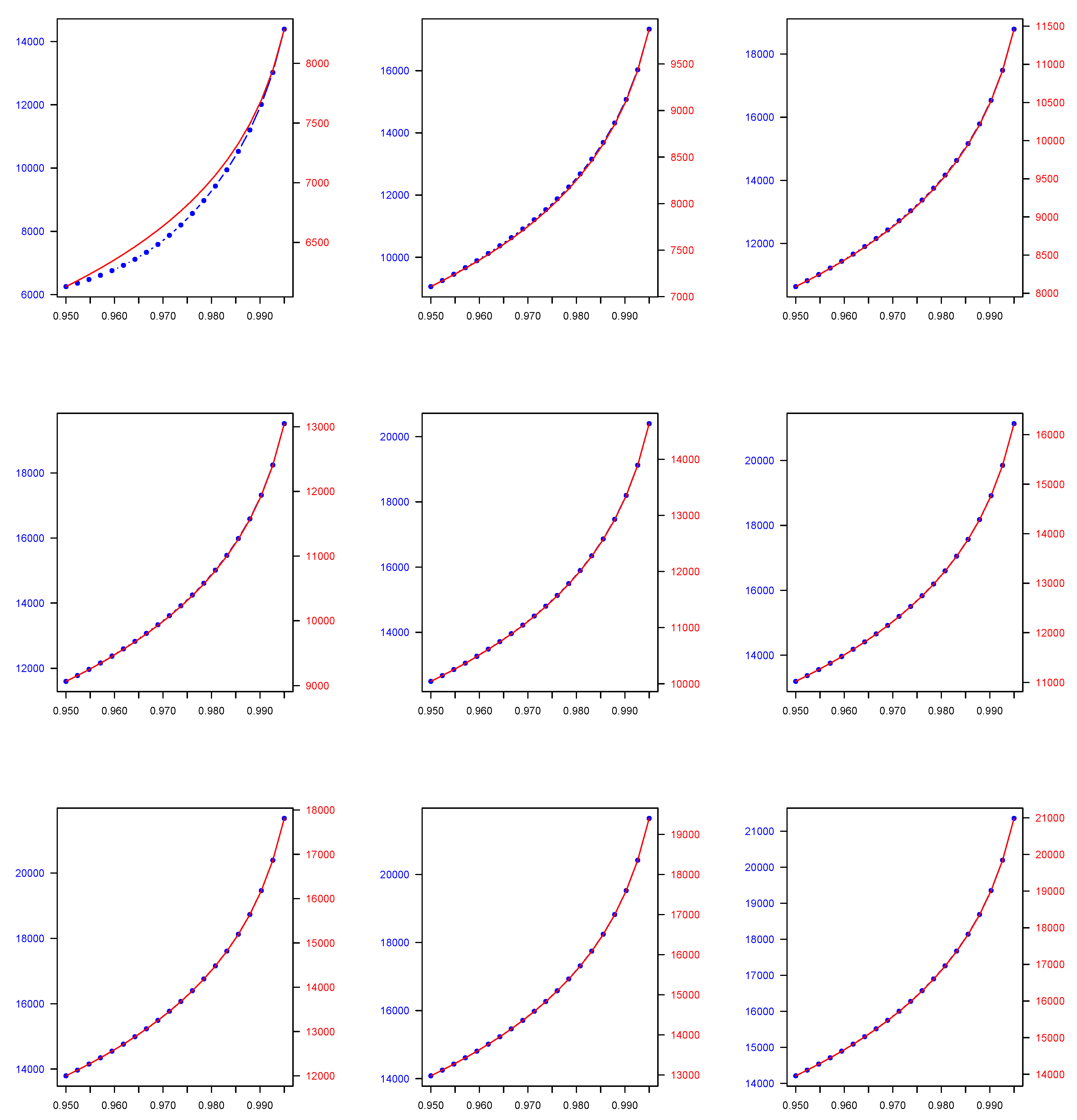
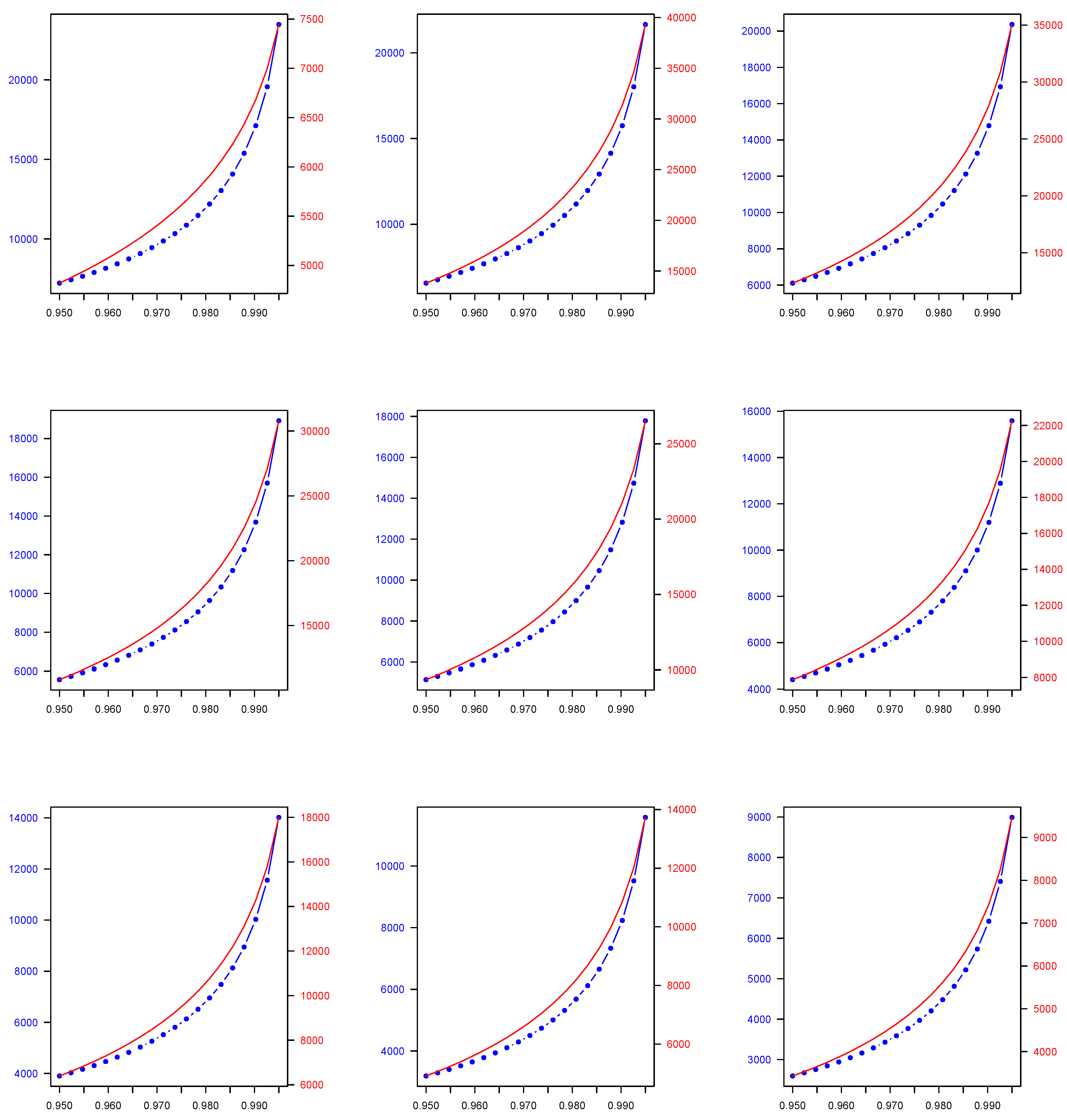
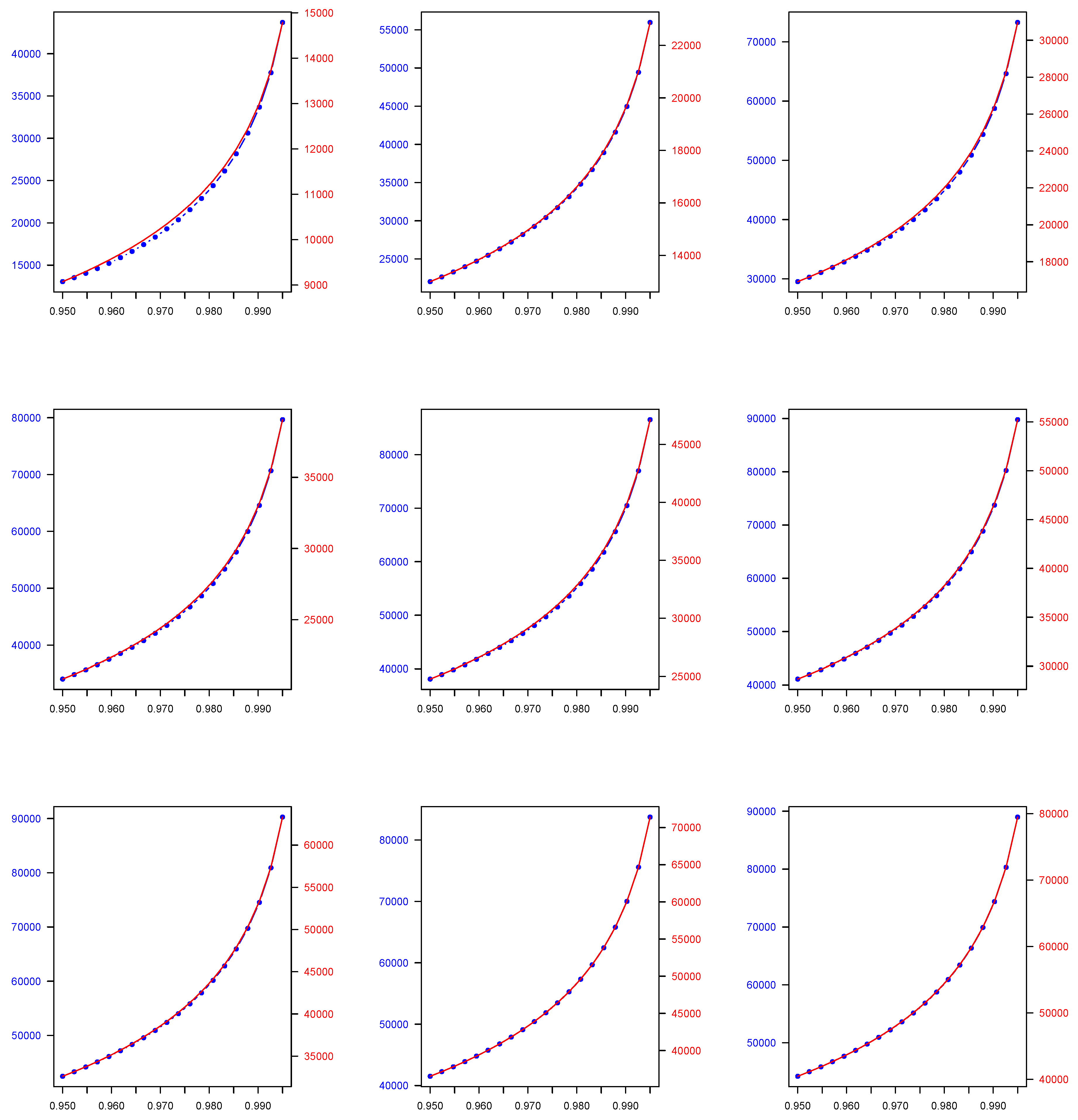
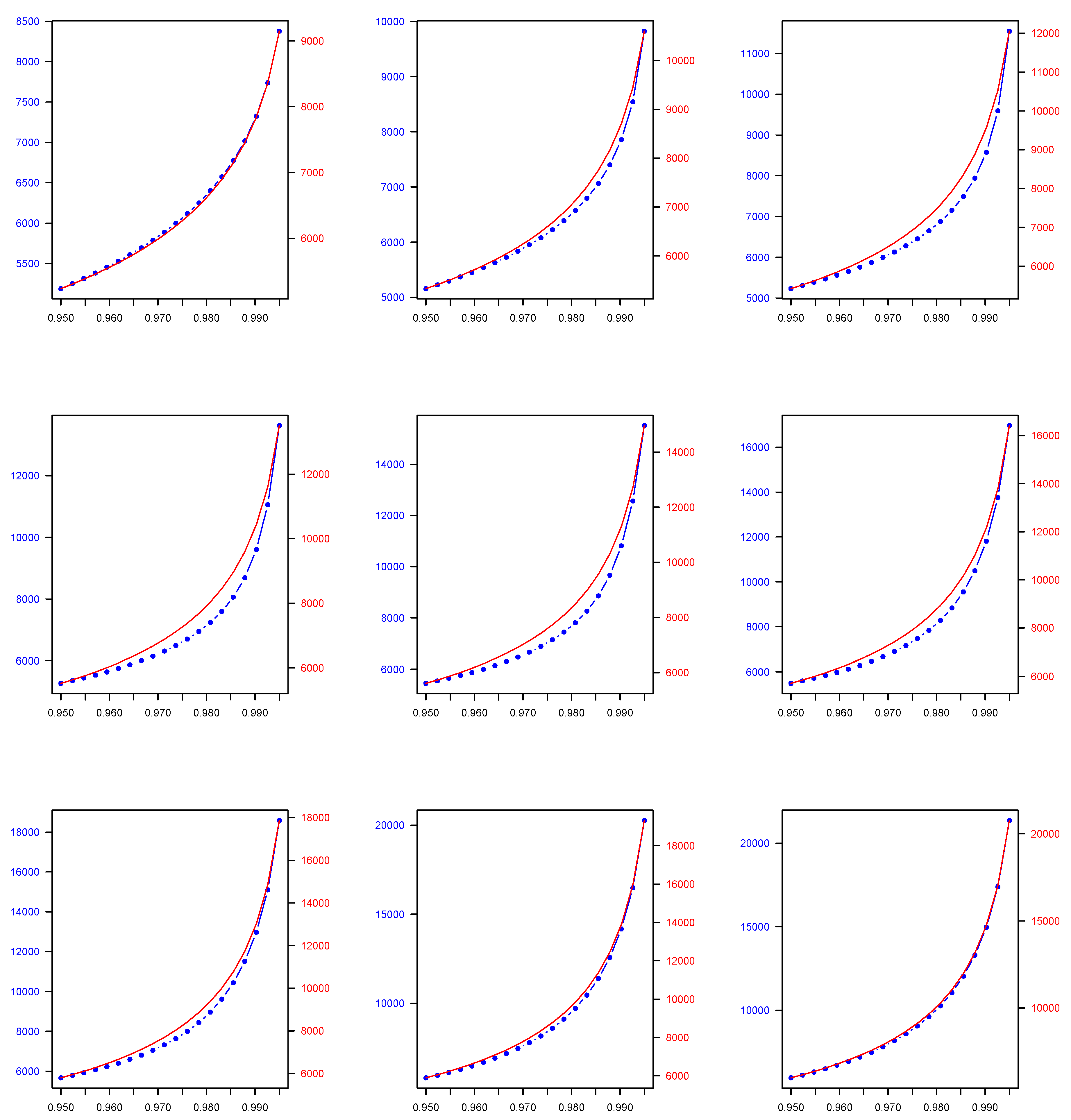
The results of our numerical application for each of the 2C component mixture models we consider in this study, namely the Normal, Gamma, Lognormal, Pareto, Lognormal-Gamma, and Pareto-Gamma, are presented in the following manner. In Table 1, for each of the previously described 2C mixture models, we show the parameters estimates across all estimated weights combinations derived using the EM algorithm. Then, in Table 2, we present the 2C mixture model-based quantiles which are computed by utilising the EM algorithm parameter and weight estimates, which are presented in Table 1, as well as the quantiles derived by using the weighted average approach across all weights combinations that are used to generate the data. Both quantile types are calculated at two widely used, in a financial context, probability levels (), i.e., 0.950 and 0.990. Finally, in Figure 1, Figure 2, Figure 3, Figure 4, Figure 5 and Figure 6, we plot the mixture-model-based quantiles and the weighted average-based quantiles computed at a more extended range of () probability levels ranging from 0.950 to 0.995. It is important to mention that the values for the two quantile types of interest appear to be substantially different, and therefore we deemed it necessary to have two distinct y axes in each plot of Figure 1, Figure 2, Figure 3, Figure 4, Figure 5 and Figure 6 to allow for an easier comparison.
As we observe, the quantile values in the case of the 2C Normal, 2C Gamma, 2C Lognormal, and 2C Pareto mixtures, and also the 2C Lognormal-Gamma and 2C Pareto-Gamma mixtures, are higher than the weighted-average-based ones. Regarding the decision-making problem we address, as was previously mentioned, the approach we consider is more flexible because it provides a two-fold benefit to the decision maker, since, in addition to enabling them to evaluate the efficacy of the expert views aggregation process, it allows them to test how the weights that they were intending to allocate to each expert opinion based on their personal judgement compared to the ones estimated by the model.
5. Concluding Remarks
When making a decision in an uncertain environment, an agent may consult multiple experts. In such a scenario, the aggregation of individual opinions before reaching a decision is required. In this study, we contribute to the plethora of interdisciplinary literature on this topic by proposing a finite mixture modelling approach that can enable the agent to combine the component distributions in order to obtain a single distribution of the quantity of interest that is a quantile-based risk measure. The component distributions we consider in this study can be used in practice to model various quantities of interest in financial and insurance applications such as financial returns and insurance losses with light and heavy tails. The suggested method allows for considerable flexibility in expert opinions regarding the distribution class of the random quantity of interest and its parameters, and it also provides an efficient way for weights computation—a task recognised as being particularly strenuous in this segment of literature. By employing the perspective that opinions take the form of quantiles, we compare our approach to the traditional weighted average one, and we find that they lead to different results. Furthermore, the proposed models can be used for carrying out different tasks in insurance such as calculating premiums and reserves and measuring tail risk.
A compelling direction of further research would be to use combinations of finite mixtures and composite models that can mitigate instabilities of tail index estimations inherited by finite mixture models; see, for instance, Fung et al. (2021). Furthermore, a natural extension of our study is to employ Bayesian inference for mixtures, which will allow us to combine internal data, external data, and expert opinions proceeding along similar lines as in Lambrigger et al. (2009). Additionally, in this paper, we have focused only on the opinion aggregation process without considering how experts have elicited their views; therefore, it would be interesting to examine ways in which this aspect is also taken into account. Finally, another potential topic of interest, with regards to weights allocation this time, is for the weights to reflect the risk aversion level of the agent as well as the quality of a given expert’s judgement, and the level of disagreement between experts.
Author Contributions
Conceptualization, D.M. and P.B.; methodology, D.M., P.B. and G.T.; software, D.M. and G.T.; formal analysis, D.M., P.B. and G.T.; investigation, D.M., P.B. and G.T.; writing—original draft preparation, D.M.; writing—review and editing, D.M. and G.T.; supervision, P.B. and G.T. All authors have read and agreed to the published version of the manuscript.
Funding
This research received no external funding.
Conflicts of Interest
The authors declare no conflict of interest.
Abbreviations
The following abbreviations are used in this manuscript:
| EM | Expectation Maximization |
| ML | Maximum Likelihood |
| Value at Risk | |
| Tail Value at Risk | |
| 2C | Two component |
| Probability density function |
References
- Acciaio, Beatrice, and Irina Penner. 2011. Dynamic risk measures. In Advanced Mathematical Methods for Finance. Berlin/Heidelberg: Springer, pp. 1–34. [Google Scholar]
- Allison, David B., Gary L. Gadbury, Moonseong Heo, José R. Fernández, Cheol-Koo Lee, Tomas A. Prolla, and Richard Weindruch. 2002. A mixture model approach for the analysis of microarray gene expression data. Computational Statistics & Data Analysis 9: 1–20. [Google Scholar]
- Bamber, Jonathan L., Willy P. Aspinall, and Roger M. Cooke. 2016. A commentary on “how to interpret expert judgment assessments of twenty-first century sea-level rise” by Hylke de Vries and Roderik SW van de Wal. Climatic Change 137: 321–28. [Google Scholar] [CrossRef] [Green Version]
- Bansal, Saurabh, and Asa Palley. 2017. Is it better to elicit quantile or probability judgments? A comparison of direct and calibrated procedures for estimating a continuous distribution. In A Comparison of Direct and Calibrated Procedures for Estimating a Continuous Distribution (6 June 2017). Kelley School of Business Research Paper. Bloomington: Indiana University, pp. 17–44. [Google Scholar]
- Barrieu, Pauline, and Claudia Ravanelli. 2015. Robust capital requirements with model risk. Economic Notes: Review of Banking, Finance and Monetary Economics 44: 1–28. [Google Scholar] [CrossRef]
- Barrieu, Pauline, and Giacomo Scandolo. 2015. Assessing financial model risk. European Journal of Operational Research 242: 546–56. [Google Scholar] [CrossRef] [Green Version]
- Barrieu, Pauline, and Nicole El Karoui. 2005. Inf-convolution of risk measures and optimal risk transfer. Finance and Stochastics 9: 269–98. [Google Scholar] [CrossRef] [Green Version]
- Bermúdez, Lluís, Dimitris Karlis, and Isabel Morillo. 2020. Modelling unobserved heterogeneity in claim counts using finite mixture models. Risks 8: 10. [Google Scholar] [CrossRef] [Green Version]
- Blostein, Martin, and Tatjana Miljkovic. 2019. On modeling left-truncated loss data using mixtures of distributions. Insurance: Mathematics and Economics 85: 35–46. [Google Scholar] [CrossRef]
- Bogner, Konrad, Katharina Liechti, and Massimiliano Zappa. 2017. Combining quantile forecasts and predictive distributions of streamflows. Hydrology and Earth System Sciences 21: 5493–502. [Google Scholar] [CrossRef] [Green Version]
- Bolger, Donnacha, and Brett Houlding. 2016. Reliability updating in linear opinion pooling for multiple decision makers. Proceedings of the Institution of Mechanical Engineers, Part O: Journal of Risk and Reliability 230: 309–22. [Google Scholar] [CrossRef]
- Bouguila, Nizar. 2010. Count data modeling and classification using finite mixtures of distributions. IEEE Transactions on Neural Networks 22: 186–98. [Google Scholar] [CrossRef]
- Bühlmann, Hans, and Alois Gisler. 2006. A Course in Credibility Theory and Its Applications. Zurich: Springer Science & Business Media. [Google Scholar]
- Busetti, Fabio. 2017. Quantile aggregation of density forecasts. Oxford Bulletin of Economics and Statistics 79: 495–512. [Google Scholar] [CrossRef]
- Caravagna, Giulio, Timon Heide, Marc J. Williams, Luis Zapata, Daniel Nichol, Ketevan Chkhaidze, William Cross, George D. Cresswell, Benjamin Werner, Ahmet Acar, and et al. 2020. Subclonal reconstruction of tumors by using machine learning and population genetics. Nature Genetics 52: 898–907. [Google Scholar] [CrossRef]
- Chai Fung, Tsz, Andrei L. Badescu, and X. Sheldon Lin. 2019. A class of mixture of experts models for general insurance: Application to correlated claim frequencies. ASTIN Bulletin 49: 647–88. [Google Scholar] [CrossRef]
- Clemen, Robert T. 1989. Combining forecasts: A review and annotated bibliography. International Journal of Forecasting 5: 559–83. [Google Scholar] [CrossRef]
- Clemen, Robert T. 2008. Comment on cooke’s classical method. Reliability Engineering & System Safety 93: 760–5. [Google Scholar]
- Clemen, Robert T., and Robert L. Winkler. 1999. Combining probability distributions from experts in risk analysis. Risk Analysis 19: 187–203. [Google Scholar] [CrossRef]
- Clemen, Robert T., and Robert L. Winkler. 2007. Aggregating Probability Distributions. Cambridge: Cambridge University Press, pp. 154–76. [Google Scholar] [CrossRef]
- Colson, Abigail R., and Roger M. Cooke. 2017. Cross validation for the classical model of structured expert judgment. Reliability Engineering & System Safety 163: 109–20. [Google Scholar]
- Cooke, Roger. 1991. Experts in Uncertainty: Opinion and Subjective Probability in Science. Oxford: Oxford University Press on Demand. [Google Scholar]
- Cooke, Roger M., and Louis L. H. J. Goossens. 2008. Tu delft expert judgment data base. Reliability Engineering & System Safety 93: 657–74. [Google Scholar]
- Couvreur, Christophe. 1997. The EM algorithm: A guided tour. In Computer Intensive Methods in Control and Signal Processing. Boston: Birkhäuser, pp. 209–22. [Google Scholar]
- Dalkey, Norman C. 1969. The Delphi Method: An Experimental Study of Group Opinion. Technical Report. Santa Monica: RAND Corporation. [Google Scholar]
- Danielsson, Jon, Paul Embrechts, Charles Goodhart, Con Keating, Felix Muennich, Olivier Renault, and Hyun Song Shin. 2001. An Academic Response to Basel II. Zurich: FMG. [Google Scholar]
- Delbecq, Andre L., Andrew H. Van de Ven, and David H. Gustafson. 1975. Group Techniques for Program Planning: A Guide to Nominal Group and Delphi Processes. Glenview: Scott Foresman. [Google Scholar]
- Dempster, Arthur P., Nan M. Laird, and Donald B. Rubin. 1977. Maximum likelihood from incomplete data via the em algorithm. Journal of the Royal Statistical Society: Series B (Methodological) 39: 1–22. [Google Scholar]
- Efron, Bradley. 2008. Microarrays, empirical bayes and the two-groups model. Statistical Science 23: 1–22. [Google Scholar]
- Eggstaff, Justin W., Thomas A. Mazzuchi, and Shahram Sarkani. 2014a. The development of progress plans using a performance-based expert judgment model to assess technical performance and risk. Systems Engineering 17: 375–91. [Google Scholar] [CrossRef]
- Eggstaff, Justin W., Thomas A. Mazzuchi, and Shahram Sarkani. 2014b. The effect of the number of seed variables on the performance of cooke’s classical model. Reliability Engineering & System Safety 121: 72–82. [Google Scholar]
- Elguebaly, Tarek, and Nizar Bouguila. 2014. Background subtraction using finite mixtures of asymmetric gaussian distributions and shadow detection. Machine Vision and Applications 25: 1145–62. [Google Scholar] [CrossRef]
- Embrechts, Paul, Giovanni Puccetti, Ludger Rüschendorf, Ruodu Wang, and Antonela Beleraj. 2014. An academic response to basel 3.5. Risks 2: 25–48. [Google Scholar] [CrossRef] [Green Version]
- Everitt, Brian S., and David J. Hand. 1981. Finite mixture distributions. In Monographs on Applied Probability and Statistics. London and New York: Chapman and Hall. [Google Scholar]
- Flandoli, Franco, Enrico Giorgi, William P. Aspinall, and Augusto Neri. 2011. Comparison of a new expert elicitation model with the classical model, equal weights and single experts, using a cross-validation technique. Reliability Engineering & System Safety 96: 1292–310. [Google Scholar]
- Föllmer, Hans, and Alexander Schied. 2010. Convex and Coherent Risk Measures. Journal of Quantitative Finance. 12. Available online: https://www.researchgate.net/publication/268261458_Convex_and_coherent_risk_measures (accessed on 8 June 2021).
- Föllmer, Hans, and Alexander Schied. 2016. Stochastic Finance: An Introduction in Discrete Time. Berlin: De Gruyter. [Google Scholar]
- Forgy, Edward W. 1965. Cluster analysis of multivariate data: Efficiency versus interpretability of classifications. Biometrics 21: 768–69. [Google Scholar]
- French, Simon. 1983. Group Consensus Probability Distributions: A Critical Survey. Manchester: University of Manchester. [Google Scholar]
- Fung, Tsz Chai, George Tzougas, and Mario Wuthrich. 2021. Mixture composite regression models with multi-type feature selection. arXiv arXiv:2103.07200. [Google Scholar]
- Gambacciani, Marco, and Marc S. Paolella. 2017. Robust normal mixtures for financial portfolio allocation. Econometrics and Statistics 3: 91–111. [Google Scholar] [CrossRef]
- Genest, Christian. 1992. Vincentization revisited. The Annals of Statistics 20: 1137–42. [Google Scholar] [CrossRef]
- Genest, Christian, and Kevin J. McConway. 1990. Allocating the weights in the linear opinion pool. Journal of Forecasting 9: 53–73. [Google Scholar] [CrossRef]
- Genest, Christian, Samaradasa Weerahandi, and James V. Zidek. 1984. Aggregating opinions through logarithmic pooling. Theory and Decision 17: 61–70. [Google Scholar] [CrossRef]
- Gneiting, Tilmann, and Adrian E. Raftery. 2007. Strictly proper scoring rules, prediction, and estimation. Journal of the American Statistical Association 102: 359–78. [Google Scholar] [CrossRef]
- Government Office for Science. 2020. Transparency Data List of Participants of Sage and Related Sub-Groups. London: Government Office for Science. [Google Scholar]
- Grün, Bettina, and Friedrich Leisch. 2008. Finite mixtures of generalized linear regression models. In Recent Advances in Linear Models and Related Areas. Heidelberg: Physica-Verlag, pp. 205–30. [Google Scholar]
- Henry, Marc, Yuichi Kitamura, and Bernard Salanié. 2014. Partial identification of finite mixtures in econometric models. Quantitative Economics 5: 123–44. [Google Scholar] [CrossRef]
- Hogarth, Robert M. 1977. Methods for aggregating opinions. In Decision Making and Change in Human Affairs. Dordrecht: Springer, pp. 231–55. [Google Scholar]
- Hora, Stephen C., Benjamin R. Fransen, Natasha Hawkins, and Irving Susel. 2013. Median aggregation of distribution functions. Decision Analysis 10: 279–91. [Google Scholar] [CrossRef] [Green Version]
- Johnson, Norman L., Samuel Kotz, and Narayanaswamy Balakrishnan. 1994. Continuous Univariate Distributions. Models and Applications, 2nd ed. New York: John Wiley & Sons. [Google Scholar]
- Jose, Victor Richmond R., Yael Grushka-Cockayne, and Kenneth C. Lichtendahl Jr. 2013. Trimmed opinion pools and the crowd’s calibration problem. Management Science 60: 463–75. [Google Scholar] [CrossRef]
- Kaplan, Stan. 1992. ‘expert information’versus ‘expert opinions’. another approach to the problem of eliciting/combining/using expert knowledge in pra. Reliability Engineering & System Safety 35: 61–72. [Google Scholar]
- Karlis, Dimitris, and Evdokia Xekalaki. 1999. Improving the em algorithm for mixtures. Statistics and Computing 9: 303–7. [Google Scholar] [CrossRef]
- Karlis, Dimitris, and Evdokia Xekalaki. 2005. Mixed poisson distributions. International Statistical Review/Revue Internationale de Statistique 73: 35–58. [Google Scholar] [CrossRef]
- Koksalmis, Emrah, and Özgür Kabak. 2019. Deriving decision makers’ weights in group decision making: An overview of objective methods. Information Fusion 49: 146–60. [Google Scholar] [CrossRef]
- Lambrigger, Dominik D., Pavel V. Shevchenko, and Mario V. Wüthrich. 2009. The quantification of operational risk using internal data, relevant external data and expert opinions. arXiv arXiv:0904.1361. [Google Scholar] [CrossRef]
- Lichtendahl, Kenneth C., Yael Grushka-Cockayne, and Robert L. Winkler. 2013. Is it better to average probabilities or quantiles? Management Science 59: 1594–611. [Google Scholar] [CrossRef]
- Linstone, Harold A., and Murray Turoff. 1975. The Delphi Method. Reading: Addison-Wesley Reading. [Google Scholar]
- MacQueen, James. 1967. Some methods for classification and analysis of multivariate observations. Paper presented at the fifth Berkeley Symposium on Mathematical Statistics and Probability, Oakland, CA, USA, January 1; vol. 1, pp. 281–97. [Google Scholar]
- Maitra, Ranjan. 2009. Initializing partition-optimization algorithms. IEEE/ACM Transactions on Computational Biology and Bioinformatics 6: 144–57. [Google Scholar] [CrossRef] [PubMed] [Green Version]
- McLachlan, Geoffrey J., and David Peel. 2000a. Finite Mixture Models. New York: John Wiley & Sons. [Google Scholar]
- McLachlan, Geoffrey J., and David Peel. 2000b. Finite Mixture Models. New York: Wiley Series in Probability and Statistics. [Google Scholar]
- McLachlan, Geoffrey J., and Kaye E. Basford. 1988. Mixture Models: Inference and Applications to Clustering. New York: M. Dekker, vol. 38. [Google Scholar]
- McLachlan, Geoffrey J., Kim-Anh Do, and Christophe Ambroise. 2005. Analyzing Microarray Gene Expression Data. Hoboken: John Wiley & Sons, vol. 422. [Google Scholar]
- McLachlan, Geoffrey J., Sharon X. Lee, and Suren I. Rathnayake. 2019. Finite mixture models. Annual Review of Statistics and Its Application 6: 355–78. [Google Scholar] [CrossRef]
- McNichols, Maureen. 1988. A comparison of the skewness of stock return distributions at earnings and non-earnings announcement dates. Journal of Accounting and Economics 10: 239–73. [Google Scholar] [CrossRef]
- Mengersen, Kerrie L., Christian Robert, and Mike Titterington. 2011. Mixtures: Estimation and Applications. Chichester: John Wiley & Sons, vol. 896. [Google Scholar]
- Miljkovic, Tatjana, and Bettina Grün. 2016. Modeling loss data using mixtures of distributions. Insurance: Mathematics and Economics 70: 387–96. [Google Scholar] [CrossRef]
- Newcomb, Simon. 1886. A generalized theory of the combination of observations so as to obtain the best result. American Journal of Mathematics 8: 343–66. [Google Scholar] [CrossRef] [Green Version]
- Oboh, Bromensele Samuel, and Nizar Bouguila. 2017. Unsupervised learning of finite mixtures using scaled dirichlet distribution and its application to software modules categorization. Paper presented at the 2017 IEEE International Conference on Industrial Technology (ICIT), Toronto, ON, Canada, March 22–25; pp. 1085–90. [Google Scholar]
- O’Hagan, Anthony, Caitlin E. Buck, Alireza Daneshkhah, J. Richard Eiser, Paul H. Garthwaite, David J. Jenkinson, Jeremy E. Oakley, and Tim Rakow. 2006. Uncertain Judgements: Eliciting Experts’ Probabilities. Chichester: John Wiley & Sons. [Google Scholar]
- Parenté, Frederik J., and Janet K. Anderson-Parenté. 1987. Delphi inquiry systems. Judgmental Forecasting, 129–56. [Google Scholar]
- Pearson, Karl. 1894. Contributions to the mathematical theory of evolution. Philosophical Transactions of the Royal Society of London. A 185: 71–110. [Google Scholar]
- Peiro, Amado. 1999. Skewness in financial returns. Journal of Banking & Finance 23: 847–62. [Google Scholar]
- Plous, Scott. 1993. The Psychology of Judgment and Decision Making. New York: Mcgraw-Hill Book Company. [Google Scholar]
- Punzo, Antonio, Angelo Mazza, and Antonello Maruotti. 2018. Fitting insurance and economic data with outliers: A flexible approach based on finite mixtures of contaminated gamma distributions. Journal of Applied Statistics 45: 2563–84. [Google Scholar] [CrossRef]
- Rufo, M. J., C. J. Pérez, and Jacinto Martín. 2010. Merging experts’ opinions: A bayesian hierarchical model with mixture of prior distributions. European Journal of Operational Research 207: 284–89. [Google Scholar] [CrossRef]
- Samadani, Ramin. 1995. A finite mixtures algorithm for finding proportions in sar images. IEEE Transactions on Image Processing 4: 1182–86. [Google Scholar] [CrossRef] [PubMed]
- Schlattmann, Peter. 2009. Medical Applications of Finite Mixture Models. Berlin/Heidelberg: Springer. [Google Scholar]
- Shevchenko, Pavel V., and Mario V. Wüthrich. 2006. The structural modelling of operational risk via bayesian inference: Combining loss data with expert opinions. The Journal of Operational Risk 1: 3–26. [Google Scholar] [CrossRef]
- Stone, Mervyn. 1961. The linear opinion pool. The Annals of Mathematical Statistics 32: 1339–42. [Google Scholar] [CrossRef]
- Titterington, D. M. 1990. Some recent research in the analysis of mixture distributions. Statistics 21: 619–41. [Google Scholar] [CrossRef]
- Titterington, D. Michael, Adrian F. M. Smith, and Udi E. Makov. 1985. Statistical Analysis of Finite Mixture Distributions. Chichester: Wiley. [Google Scholar]
- Tzougas, George, Spyridon Vrontos, and Nicholas Frangos. 2014. Optimal bonus-malus systems using finite mixture models. Astin Bulletin 44: 417–44. [Google Scholar] [CrossRef] [Green Version]
- Tzougas, George, Spyridon Vrontos, and Nicholas Frangos. 2018. Bonus-malus systems with two-component mixture models arising from different parametric families. North American Actuarial Journal 22: 55–91. [Google Scholar] [CrossRef]
- Vincent, Stella Burnham. 1912. The functions of the Vibrissae in the Behavior of the White Rat. Chicago: University of Chicago, vol. 1. [Google Scholar]
- Wallach, Michael A., Nathan Kogan, and Daryl J. Bem. 1962. Group influence on individual risk taking. The Journal of Abnormal and Social Psychology 65: 75. [Google Scholar] [CrossRef] [Green Version]
- Wedel, Michel, and Wayne S. DeSarbo. 1994. A review of recent developments in latent class regression models. In Advanced Methods of Marketing Research. Edited by Richard Bagozzi. Oxford: Blackwell Publishing Ltd., pp. 352–88. [Google Scholar]
- Winkler, Robert L. 1968. The consensus of subjective probability distributions. Management Science 15: B-61. [Google Scholar] [CrossRef]
- Winkler, Robert L., Javier Munoz, José L. Cervera, José M. Bernardo, Gail Blattenberger, Joseph B. Kadane, Dennis V. Lindley, Allan H. Murphy, Robert M. Oliver, and David Ríos-Insua. 1996. Scoring rules and the evaluation of probabilities. Test 5: 1–60. [Google Scholar] [CrossRef]
- Yung, Yiu-Fai. 1997. Finite mixtures in confirmatory factor-analysis models. Psychometrika 62: 297–330. [Google Scholar] [CrossRef]
Figure 1.
Two-component (2C) Normal finite mixture model-based () quantile (blue colour) across all () combinations versus two-component (2C) Normal weighted average-based () quantile (red colour) across all () combinations, where () takes values in the range of 0.950-0.995. Note that, due to a considerable discrepancy between and values, each given plot has two different y axes—one for each quantile type.

Figure 2.
Two-Component (2C) Lognormal finite mixture model-based () quantile (blue colour) across all () combinations versus two-component (2C) Lognormal weighted average-based () quantile (red colour) across all () combinations, where () takes values in the range of 0.950-0.995. Note that, due to a considerable discrepancy between and values, each given plot has two different y axes—one for each quantile type.

Figure 3.
Two-Component (2C) Gamma finite mixture model-based () quantile (blue colour) across all () combinations versus two-component (2C) Gamma weighted average-based () quantile (red colour) across all () combinations, where () takes values in the range of 0.950-0.995. Note that, due to a considerable discrepancy between and values, each given plot has two different y axes—one for each quantile type.

Figure 4.
Two-Component (2C) Pareto finite mixture model-based () quantile (blue colour) across all () combinations versus two-component (2C) Pareto weighted average-based () quantile (red colour) across all () combinations, where () takes values in the range of 0.950-0.995. Note that, due to a considerable discrepancy between and values, each given plot has two different y axes—one for each quantile type.

Figure 5.
Two-Component (2C) Lognormal-Gamma finite mixture model-based () quantile (blue colour) across all () combinations versus two-component (2C) Lognormal-Gamma weighted average-based () quantile (red colour) across all () combinations, where () takes values in the range of 0.950-0.995. Note that, due to a considerable discrepancy between and values, each given plot has two different y axes-one for each quantile type.

Figure 6.
Two-Component (2C) Pareto-Gamma finite mixture model-based () quantile (blue colour) across all () combinations versus two-component (2C) Pareto-Gamma weighted average-based () quantile (red colour) across all () combinations, where () takes values in the range of 0.950-0.995. Note that, due to a considerable discrepancy between and values, each given plot has two different y axes—one for each quantile type.


Table 1.
EM algorithm estimates for various two-component (2C) finite mixture models. Estimates refer to the parameters mean () and standard deviation (, ) and the mixing weights of each mixture component (, ) across all plausible mixing weight combinations () in the true data generative process. All estimates provided are statistically significant at a threshold or below.
| Parametric Family | ||||||
| 0.098 | 0.902 | 5271.210 | 1333.022 | 0.228 | 0.442 | |
| 0.203 | 0.797 | 5273.012 | 1342.762 | 0.231 | 0.448 | |
| 0.300 | 0.700 | 5272.341 | 1341.234 | 0.225 | 0.448 | |
| 0.400 | 0.600 | 5271.032 | 1340.012 | 0.221 | 0.446 | |
| 2C Normal | 0.500 | 0.500 | 5272.002 | 1342.569 | 0.230 | 0.447 |
| 0.600 | 0.400 | 5272.321 | 1343.812 | 0.238 | 0.449 | |
| 0.700 | 0.300 | 5270.921 | 1341.989 | 0.236 | 0.444 | |
| 0.800 | 0.200 | 5271.981 | 1345.091 | 0.239 | 0.449 | |
| 0.901 | 0.099 | 5273.182 | 1343.991 | 0.240 | 0.447 | |
| 0.090 | 0.910 | 9.538 | 8.042 | 0.723 | 0.884 | |
| 0.200 | 0.800 | 9.521 | 8.025 | 0.717 | 0.879 | |
| 0.299 | 0.701 | 9.539 | 8.042 | 0.772 | 0.883 | |
| 0.398 | 0.602 | 9.537 | 8.041 | 0.771 | 0.881 | |
| 2C Lognormal | 0.498 | 0.502 | 9.538 | 8.064 | 0.778 | 0.899 |
| 0.600 | 0.400 | 9.548 | 8.053 | 0.766 | 0.896 | |
| 0.700 | 0.300 | 9.528 | 8.035 | 0.741 | 0.873 | |
| 0.802 | 0.198 | 9.508 | 0.722 | 8.016 | 0.858 | |
| 0.901 | 0.099 | 9.511 | 0.733 | 8.023 | 0.867 | |
| 0.086 | 0.914 | 6786.348 | 3162.126 | 0.625 | 0.352 | |
| 0.207 | 0.793 | 6737.558 | 3127.165 | 0.629 | 0.340 | |
| 0.307 | 0.693 | 6738.557 | 3124.408 | 0.635 | 0.342 | |
| 0.400 | 0.600 | 6739.659 | 3127.512 | 0.629 | 0.344 | |
| 2C Gamma | 0.499 | 0.501 | 6784.309 | 3171.627 | 0.630 | 0.357 |
| 0.601 | 0.399 | 6754.742 | 3123.512 | 0.638 | 0.341 | |
| 0.700 | 0.300 | 6783.127 | 3170.006 | 0.636 | 0.346 | |
| 0.799 | 0.201 | 6783.021 | 3172.871 | 0.621 | 0.341 | |
| 0.902 | 0.098 | 6786.735 | 3172.513 | 0.599 | 0.343 | |
| 0.088 | 0.912 | 1364.138 | 3148.568 | 3.354 | 2.439 | |
| 0.204 | 0.796 | 1329.177 | 3099.778 | 3.342 | 2.442 | |
| 0.295 | 0.705 | 1326.426 | 3100.769 | 3.344 | 2.448 | |
| 0.405 | 0.595 | 1329.524 | 3101.871 | 3.346 | 2.443 | |
| 2C Pareto | 0.494 | 0.506 | 1373.639 | 3146.521 | 3.359 | 2.444 |
| 0.605 | 0.395 | 1325.524 | 3116.954 | 3.343 | 2.452 | |
| 0.694 | 0.306 | 1372.018 | 3145.339 | 3.348 | 2.450 | |
| 0.805 | 0.195 | 1374.883 | 3145.233 | 3.343 | 2.434 | |
| 0.896 | 0.104 | 1374.525 | 3148.947 | 3.345 | 2.422 | |
| 0.088 | 0.912 | 1902.904 | 2393.673 | 2.085 | 0.604 | |
| 0.204 | 0.796 | 1867.943 | 2344.883 | 2.073 | 0.608 | |
| 0.295 | 0.705 | 1865.186 | 2345.882 | 2.075 | 0.614 | |
| 0.404 | 0.596 | 1868.129 | 2346.984 | 2.077 | 0.608 | |
| 2C Lognormal-Gamma | 0.494 | 0.506 | 1912.405 | 2391.634 | 2.079 | 0.609 |
| 0.605 | 0.395 | 1864.289 | 2362.067 | 2.074 | 0.617 | |
| 0.694 | 0.306 | 1910.784 | 2390.452 | 2.079 | 0.615 | |
| 0.805 | 0.195 | 1913.649 | 2394.123 | 2.074 | 0.602 | |
| 0.896 | 0.104 | 1912.018 | 2396.106 | 2.076 | 0.599 | |
| 0.088 | 0.912 | 9.538 | 3175.526 | 0.725 | 0.737 | |
| 0.197 | 0.803 | 9.522 | 3140.588 | 0.722 | 0.741 | |
| 0.297 | 0.703 | 9.543 | 3139.065 | 0.781 | 0.747 | |
| 0.396 | 0.604 | 9.547 | 3142.169 | 0.777 | 0.742 | |
| 2C Pareto-Gamma | 0.496 | 0.504 | 9.547 | 3186.286 | 0.784 | 0.743 |
| 0.598 | 0.402 | 9.558 | 3138.171 | 0.772 | 0.751 | |
| 0.698 | 0.302 | 9.537 | 3184.665 | 0.765 | 0.749 | |
| 0.800 | 0.200 | 9.517 | 3187.353 | 0.728 | 0.734 | |
| 0.899 | 0.101 | 9.520 | 3189.272 | 0.739 | 0.729 |
Table 2.
Comparison between the finite mixture model-based () quantile and the weighted average-based () quantile derived for the various parametric families considered in this study. Note that () denotes the probability level at which the quantile is computed. The quantile is calculated by using the derived EM parameters and weights estimates shown in Table 1. For the computation of quantile , no model estimation is involved, and it is calculated as the weighted average of two individual quantiles, each coming from a distribution family with parameters and weights as those used to generate the data.
| Finite Mixture Model-Based Quantile | ||||||
|---|---|---|---|---|---|---|
| 2C Normal | 2C Lognormal | 2C Gamma | 2C Pareto | 2C Lognormal-Gamma | 2C Pareto-Gamma | |
| 0.950 | 5271.204 | 18,674.230 | 6254.920 | 7221.820 | 13,053.610 | 5189.413 |
| 0.990 | 5271.499 | 37,254.660 | 11,911.220 | 16,895.230 | 33,302.150 | 7286.269 |
| 0.950 | 5273.171 | 24,144.120 | 9057.693 | 6569.990 | 22,039.780 | 5157.749 |
| 0.990 | 5273.394 | 45,694.640 | 14,982.950 | 15,542.580 | 44,546.370 | 7797.691 |
| 0.950 | 5272.559 | 30,361.480 | 10,637.600 | 6108.752 | 29,534.510 | 5231.247 |
| 0.990 | 5272.754 | 57,847.270 | 16,443.240 | 14,589.80 | 58,206.920 | 8493.526 |
| 0.950 | 5271.286 | 34,225.830 | 11,600.840 | 5564.221 | 34,066.590 | 5273.603 |
| 0.990 | 5271.465 | 63,167.590 | 17,229.970 | 13,503.800 | 63,994.280 | 9481.466 |
| 0.950 | 5272.297 | 38,063.000 | 12,505.360 | 5147.291 | 38,106.660 | 5449.650 |
| 0.990 | 5272.474 | 68,905.430 | 18,108.690 | 12,655.920 | 69,880.110 | 10,662.670 |
| 0.950 | 5272.650 | 40,758.710 | 13,203.380 | 4409.509 | 41,120.820 | 5487.197 |
| 0.990 | 5272.827 | 71,836.230 | 18,826.360 | 11,044.520 | 73,116.860 | 11,643.710 |
| 0.950 | 5271.267 | 40,870.610 | 13,793.70 | 3904.314 | 42,478.650 | 5662.312 |
| 0.990 | 5271.438 | 69,767.140 | 19,373.060 | 9889.721 | 73,938.670 | 12,784.550 |
| 0.950 | 5272.348 | 40,907.890 | 14,083.190 | 3191.665 | 41,516.230 | 5810.997 |
| 0.990 | 5272.517 | 68,097.500 | 19,440.430 | 8118.793 | 69,476.320 | 13,964.470 |
| 0.950 | 5273.564 | 43,519.640 | 14,211.730 | 2596.741 | 44,222.170 | 5958.190 |
| 0.990 | 5273.731 | 72,328.780 | 19,271.110 | 6335.289 | 73,824.540 | 14,757.320 |
| Weighted average-based quantile | ||||||
| 2C Normal | 2C Lognormal | 2C Gamma | 2C Pareto | 2C Lognormal-Gamma | 2C Pareto-Gamma | |
| 0.950 | 1713.689 | 15,847.350 | 6130.278 | 6974.334 | 9075.481 | 5234.196 |
| 0.990 | 1713.975 | 28,081.790 | 7666.813 | 16,133.486 | 12,933.270 | 7791.443 |
| 0.950 | 2106.655 | 19,018.620 | 7108.780 | 6415.912 | 12,999.186 | 5328.475 |
| 0.990 | 2106.926 | 33,072.860 | 9074.596 | 14,783.290 | 19,607.500 | 8635.935 |
| 0.950 | 2499.620 | 22,189.900 | 8087.282 | 5857.489 | 16,922.892 | 5422.755 |
| 0.990 | 2499.877 | 38,063.930 | 10,482.379 | 13,433.094 | 32,955.980 | 9480.427 |
| 0.950 | 2892.586 | 25,361.170 | 9065.785 | 5299.066 | 20,846.597 | 5517.035 |
| 0.990 | 2892.828 | 43,054.990 | 11,890.162 | 12,082.899 | 26,281.740 | 10,324.919 |
| 0.950 | 3285.551 | 28,532.450 | 10,044.287 | 4740.644 | 24,770.303 | 5611.315 |
| 0.990 | 3285.779 | 48,046.060 | 13,297.946 | 10,732.703 | 39,630.220 | 11,169.410 |
| 0.950 | 3678.516 | 31,703.730 | 11,022.790 | 4182.221 | 28,694.008 | 5705.594 |
| 0.990 | 3678.730 | 53,037.130 | 14,705.729 | 9382.508 | 46,304.450 | 12,013.902 |
| 0.950 | 4071.482 | 34,875.000 | 12,001.292 | 3623.798 | 32,617.714 | 5799.874 |
| 0.990 | 4071.682 | 58,028.200 | 16,113.512 | 8032.312 | 52,978.690 | 12,858.394 |
| 0.950 | 4464.447 | 38,046.280 | 12,979.794 | 3065.376 | 36,541.419 | 5894.154 |
| 0.990 | 4464.633 | 63,019.270 | 17,521.295 | 6682.116 | 59,652.930 | 13,702.886 |
| 0.950 | 4857.413 | 41,217.550 | 13,958.297 | 2506.953 | 40,465.125 | 5988.433 |
| 0.990 | 4857.584 | 68,010.340 | 18,929.078 | 5331.921 | 66,327.170 | 14,547.377 |
Publisher’s Note: MDPI stays neutral with regard to jurisdictional claims in published maps and institutional affiliations. |
© 2021 by the authors. Licensee MDPI, Basel, Switzerland. This article is an open access article distributed under the terms and conditions of the Creative Commons Attribution (CC BY) license (https://creativecommons.org/licenses/by/4.0/).
Share and Cite
MDPI and ACS Style
Makariou, D.; Barrieu, P.; Tzougas, G. A Finite Mixture Modelling Perspective for Combining Experts’ Opinions with an Application to Quantile-Based Risk Measures. Risks 2021, 9, 115. https://doi.org/10.3390/risks9060115
AMA Style
Makariou D, Barrieu P, Tzougas G. A Finite Mixture Modelling Perspective for Combining Experts’ Opinions with an Application to Quantile-Based Risk Measures. Risks. 2021; 9(6):115. https://doi.org/10.3390/risks9060115
Chicago/Turabian StyleMakariou, Despoina, Pauline Barrieu, and George Tzougas. 2021. "A Finite Mixture Modelling Perspective for Combining Experts’ Opinions with an Application to Quantile-Based Risk Measures" Risks 9, no. 6: 115. https://doi.org/10.3390/risks9060115
Note that from the first issue of 2016, this journal uses article numbers instead of page numbers. See further details here.