Improving Explainability of Major Risk Factors in Artificial Neural Networks for Auto Insurance Rate Regulation

Abstract

In insurance rate-making, the use of statistical machine learning techniques such as artificial neural networks (ANN) is an emerging approach, and many insurance companies have been using them for pricing. However, due to the complexity of model specification and its implementation, model explainability may be essential to meet insurance pricing transparency for rate regulation purposes. This requirement may imply the need for estimating or evaluating the variable importance when complicated models are used. Furthermore, from both rate-making and rate-regulation perspectives, it is critical to investigate the impact of major risk factors on the response variables, such as claim frequency or claim severity. In this work, we consider the modelling problems of how claim counts, claim amounts and average loss per claim are related to major risk factors. ANN models are applied to meet this goal, and variable importance is measured to improve the model’s explainability due to the models’ complex nature. The results obtained from different variable importance measurements are compared, and dominant risk factors are identified. The contribution of this work is in making advanced mathematical models possible for applications in auto insurance rate regulation. This study focuses on analyzing major risks only, but the proposed method can be applied to more general insurance pricing problems when additional risk factors are being considered. In addition, the proposed methodology is useful for other business applications where statistical machine learning techniques are used.

1. Introduction

Predictive modelling techniques have been widely used in auto insurance pricing (Xie and Lawniczak 2018; Xie 2019; Ayuso et al. 2019; Parodi 2012; Yunos et al. 2016; Yan et al. 2009) and other fields of study such as bankruptcy prevention and prediction (Kliestik et al. 2018; Kovacova et al. 2019). In auto insurance, the main reason for the prevalence of predictive modelling is their superior power in accurately pricing insurance contracts and the statistical soundness of the approaches used, mostly when auto insurance rates are regulated (Verbelen et al. 2018). If insurance rates are not regulated, then the merit of predictive modelling is still apparent as its use in pricing helps to avoid the adverse selection of insurance policies (Dionne et al. 1999). Recently, the use of machine learning techniques such as artificial neural networks (ANN) has been an emerging approach for insurance pricing. They can often achieve a high level of model prediction accuracy (Fialova and Folvarcna 2020; Gao and Wüthrich 2018; lseri and Karlık 2009; Sun et al. 2017; Wuthrich 2019; Yeo et al. 2001). When ANNs are used for pricing, the high prediction accuracy of loss costs is mainly due to its capability to model the non-linear relationships between the independent variables and the response variable. For instance, in Yunos et al. (2016), the backpropagation neural network (BPNN) model was used as a tool to model both claim frequency and claim severity. This study illustrates the capability of BPNN in explaining the non-linear relationships of loss data. Furthermore, the predictive modelling techniques of machine learning have been successfully used for detecting insurance claim fraud (Bhowmik 2011). Due to models’ natural complexity, ANN and other sophisticated models have not been heavily used by insurance companies and regulators. From the rate regulation perspective, the major downside of using ANN is its low explainability due to the iterative nature of the neural network algorithms and the non-closed form, non-linear relationships between input variables and the output response. Thus, insurance companies often have difficulty explaining the model output, so the justification of methodologies’ appropriateness becomes challenging. It is often difficult to derive the risk relativities for risk factors when using ANNs due to non-linearity among the risk factors and the complex nature of ANNs. It is also hard to obtain consistent estimates of risk factors’ impact on the model response, which different network architectures may cause. Therefore, an ANN model is often treated as a black box, particularly for the multiple hidden-layer models. It provides minimal explanatory insights into the input variables’ relative influence on the output variable in the model prediction process (Olden and Jackson 2002).

Explainable artificial intelligence (AI) or explainable machine learning is now a new focus and an essential aspect when using machine learning techniques or algorithms for real-world applications (Adadi and Berrada 2018; Dosilovic et al. 2018; Samek et al. 2017; Wuthrich 2019). This concept has also played an essential role in auto insurance rate regulation. The interest in explainable AI has dramatically increased since 2016, and various review papers have been recently published. In Arrieta et al. (2020), the existing literature and contributions already made in the field of explainable AI have been surveyed. A series of challenges faced by explainable AI, including the model explainability, was also addressed. In Beaudouin et al. (2020), context-specific explainable AI was discussed using a multidisciplinary approach. However, the concept of explainability could be dated back to the 1970s when applied expert systems and rule-based models became popular (Adadi and Berrada 2018). Explainable data analytics, a sub-field of explainable AI, has recently attracted considerable attention in the machine learning community. For instance, the 2019 IEEE Symposium on Explainable Data Analytics (EDA) in Computational Intelligence is the first conference focusing on explainable data analytics. EDA aims to study suitable analytical tools, which can be used to produce information from data that facilitates decision-making or gives meaningful explanations on the impact of the input variables on the outputs in modelling. The analytical techniques in EDA include, but are not limited to, statistical measures, feature extraction, dimension reduction, and sparse methods (Lu et al. 2005; Maitra and Yan 2008; Ribeiro et al. 2006). In business intelligence for risk management, the explainability of models becomes a critical aspect as it leads to a better understanding of how the decisions are being made. The better the understanding of the models used, the more confidence and the better control of the risk, in particular for auto insurance rate-making (Hsiao et al. 1990; Kim and Canny 2018; Farbmacher et al. 2019). This is why explainable machine learning is attracting dramatic attention when machine learning techniques are used for real-world applications. The main effort to research explainable AI is to better understand the algorithms used, mathematically, statistically, or computationally, as they can be extremely complicated. This may call for methods that are able to balance the model complexity and the desired explainability of the model used.

From both insurance pricing and rate regulation perspectives, it is essential to investigate the impact of risk factors on claim frequency or claim severity (Gilenko and Mironova 2017). When a complicated mathematical model is used for pricing or capturing the loss pattern, it is critical to study the impact or conduct a sensitivity analysis of risk factors in the model (Asmussen and Rubinstein 1999). In rate regulation, the requirement of model explainability may imply the need to estimate or evaluate the importance of risk factors (Frees 1998). Different machine learning techniques and applications require different types of explainability. Algorithms used by governments are subject to higher explainability requirements (Beaudouin et al. 2020). In the machine learning community, many techniques used for capturing variable importance have been investigated. Interpretable models, including linear regression, logistic regression, generalized linear models (GLM), generalized additive models (GAM), and decision tree, have been well studied and used for evaluating variable importance due to the fact that model coefficients can be easily used for the study of the effect size of the variables. Although these models are more interpretable, they are limited in capturing more complicated non-linear relationships, which usually lack functionality. The second type of approach to study the interpretability of data is the model-agnostic method, and it has been successfully used in actuarial science (Henckaerts et al. 2020). Partial dependence plot (PDP) (Friedman 2001), permutation feature importance (Fisher et al. 2019), and shapely values (Sundararajan and Najmi 2019) are examples of the model-agnostic methods. The most significant benefit of using the agnostic approach is the flexibility of using machine learning methods, including the black box models, which are crucial for more complex real-world problems. A PDP plot shows the marginal effect of the variable on the predicted outcome of selected machine learning models, while permutation feature importance measures the increase of model error after permuting the feature variables. The model-agnostic methods provide friendly and convenient graphical tools for machine learning approaches.

In this work, we aim at improving the explainability of input factors in ANN for rate regulation purposes. We try to better understand the impact of various risk factors on statistical data reporting, which is of high-level statistical plan data (Furst et al. 2019). The statistical plan information is a crucial source for insurance regulation, and it summarizes the loss information at the industry level. However, the statistical plan data’s direct use without further processing by the mathematical model is quite limited due to its descriptive nature. Furthermore, it is difficult to know what contributes more or less to the insurance loss if only focusing on the descriptive measures in the statistical plan data reporting. Thus, it is difficult to see the driving force of insurance loss and decide the benchmark measures associated with risk factors by looking at these statistical data reports. Therefore, the benchmarks used for rate regulation are obtained by applying rate-making methodologies to these statistical plan data, typically through statistical modelling, such as GLMs, GAMs or ANNs. Unlike insurance pricing, which mainly targets the study of risk factors that significantly impact the calculation of insurance prices, we focus on major risk factors for insurance rate regulation purposes. In the current research, ANNs and their importance measures of predictors have not yet been investigated in the field of insurance rate-makings from the regulation perspective. This objective makes our contribution to the current research novel and unique. In this work, to better understand the constructed ANN models and their model outputs, we study the importance of major risk factors affecting the claim frequency and the claim severity. We consider accident year (AY), reporting year (RY), territory, coverage, and the Size-of-Loss (in terms of log-scale of the upper limit of Size-of-Loss intervals) as major risk factors. Here, the Size-of-Loss is the loss bracket, rather than the insurance loss amount caused by drivers. The level associated with this factor can be predefined based on the historical pattern of the loss data, mainly on range of loss amounts. Considering both the accident year and reporting year as risk factors, data from different accident years or other reporting years may significantly affect the analysis results. The risk affecting insurance pricing could be due to the information associated with different accident years or other reporting years. From year to year, the general level of claims may fluctuate heavily (Dugas et al. 2003). The data variability may also be due to the case reserve update for different accident years or various data reporting years. For territory, coverage, and Size-of-Loss, they are common risk factors that appear in rate regulation and are commonly used for auto insurance pricing (McClenahan 2014).

This work emphasizes measuring and interpreting the importance of risk factors using ANN. We aim to estimate and evaluate the importance of risk factors, although the modelling techniques may deal with the problem at each risk factor’s level. The significance of this work is to propose a novel approach for analyzing major risk factors, in terms of their impact to claim counts, claim amounts, and average loss per claim, for rate regulation purposes. To the best of our knowledge, this study is the first attempt to model claim counts and claim amounts using neural network models and Size-of-Loss data in the actuarial domain. This paper is organized as follows. In Section 3, the methods, including artificial neural networks and variable importance measures, are discussed. In Section 4, the obtained results using industry size of loss data are presented and analysed. Finally, we conclude our findings and provide further remarks in Section 6.

2. Data

In this work, we use datasets from the Insurance Bureau of Canada (IBC), which is a Canadian organization responsible for insurance data collections and their statistical data reporting in the area of property and casualty insurance (Xie and Chua-Chow 2020). During the data collection process, insurance companies report the loss information, including the number of claims, number of exposures, loss amounts, as well as other key information such as territories of loss, coverages, driving records associated with loss, and accident years. These statistical data are reported regularly (i.e., weekly, biweekly, or monthly). At the end of each half-year, the total claim amounts and claim counts reported by all insurance companies are aggregated by territories, coverages, accident years, etc. The statistical data reporting is then used for insurance rate regulation to ensure the premiums charged by insurance companies are fair and exact. The dataset used in this work consists of summarized claim counts, claim amount, and average loss cost by different sizes of loss, which are represented by a set of non-overlapping intervals. These summary of loss information are aggregated by major coverages, i.e., Bodily Injuries (BI) and Accident Benefits (AB). The data were also summarized by different accident years, by different report years and by different territories, i.e., Urban (U) and Rural (R).

To carry out the study, we organize data by coverages (AB and BI) and by territories (U and R). We consider the data from different reporting years and accident years as repeated observations. There are two reporting years, 2013 and 2014, respectively. There is a set of rolling most recent five years of data corresponding to five accident years for each reporting year. Therefore, for this study, we have in total ten years of observation. In addition, since we have both Accident Benefits and Bodily Injuries as the coverage type and Urban and Rural as the territory, we consider the following four different combinations, Accident Benefits and Urban (ABU), Accident Benefits and Rural (ABR), Bodily Injuries and Urban (BIU), and Bodily Injuries and Rural (BIR). These data are then formed into a data matrix with a $40\times 24$ dimension, where 40 is the total number of observations, and 24 is the number of total intervals of the Size-of-Loss.

3. Methods

In this work, we focus on improving the explainability of neural network models. We first identify the suitable model by balancing the model errors and network architecture complexities. This process is like the cross-validation procedure in the usual predictive modelling. Due to the non-linearity of neural networks, the model error does not need to decrease when increasing the network architecture. The model selection is made by searching for a suitable scale of network architecture that achieves the minimum model error within a set of small-scale neural networks and cross-validated by the root mean square error (RMSE). In this section, we mainly discuss how artificial neural networks work as a regression modelling problem. To give a more understandable explanation, we focus on the discussion of low scale neural networks. We then discuss how to measure the importance of the variables in ANN models.

3.1. Artificial Neural Networks

Let us first discuss the case of an Artificial Neural Network (ANN) with one hidden layer. That is, the network includes the input layer, one hidden layer, and the output layer. Suppose in the ANN model that there are D inputs $x_1$, $x_2$, …, $x_D$, and $M_1$ hidden units $z_1^{\left(1\right)}$, $z_2^{\left(1\right)}$, …, $z_{M_1}^{\left(1\right)}$ in the hidden layer. A unit $z_j$ within the hidden layer is defined as

$$\begin{array}{c}\hfill z_j^{\left(1\right)}=h\left(a_j^{\left(1\right)}\right)=h\left(\sum _{i=1}^D{w}_{ji}^{\left(1\right)}{x}_i+w_{j0}^{\left(1\right)}\right),\end{array}$$

(1)

where $a_j^{\left(1\right)}$ is the activation that is composed of the linear combination of input variables $x_i$, their weights $w_{ji}^{\left(1\right)}$, and the bias $w_{j0}^{\left(1\right)}$. The superscript (1) in the weights indicates that components correspond to the first hidden layer. This allows us to extend the model for multiple layers, instead of just one. The function $h(·)$ is called the activation function, which is usually non-linear and differentiable. In most cases, the activation function is chosen to be sigmoidal (Bishop 2006). If the function $h(·)$ is an identity, the hidden unit becomes a linear combination of input variables. Within this case, if we further assume that the weight values at the hidden value is a set of values resulting in a maximum variance of $z_j^{\left(1\right)}$, then $z_j^{\left(1\right)}$ is exactly the jth principal component of the inputs variable $x_1$, $x_2$,…, $x_D$. Given the hidden unit $z_j$ in the hidden layer, the resulting output unit activation $a_j^{\left(2\right)}$ in the output layer (which becomes the second hidden layer for the multiple hidden layer case) is defined as

$$\begin{array}{c}\hfill a_j^{\left(2\right)}=\sum _{i=1}^{M_1}{w}_{ji}^{\left(2\right)}{z}_i^{\left(1\right)}+w_{j0}^{\left(2\right)},\mathrm{for}j=1,\dots ,M_2,\end{array}$$

(2)

where $w_{ji}^{\left(2\right)}$ represents the weights and $w_{j0}^{\left(2\right)}$ is the bias term. The superscript (2) in the weights implies that the components correspond to the output layer or the second hidden layer if the model has multiple hidden layers. The units $z_1^{\left(2\right)}$, $z_2^{\left(2\right)}$, …, $z_{M_2}^{\left(2\right)}$ in the output layer or the second hidden layer using the same activation function $h(·)$ become

$$\begin{array}{c}\hfill z_j^{\left(2\right)}=h\left(a_j^{\left(2\right)}\right)=h\left(\sum _{i=1}^{M_1}{w}_{ji}^{\left(2\right)}{z}_i^{\left(1\right)}+w_{j0}^{\left(2\right)}\right).\end{array}$$

(3)

Let us now consider a more general case with multiple hidden layers. Assume that the total number of hidden layers is L, and there are $M_l$ hidden units $z_1^{\left(l\right)}$, $z_2^{\left(l\right)}$, …, $z_{M_l}^{\left(l\right)}$ in the lth hidden layer; we can write the $l+1$ hidden layer units as follows:

$$\begin{array}{c}\hfill z_j^{(l+1)}=h\left(a_j^{(l+1)}\right)=h\left(\sum _{i=1}^{M_l}{w}_{ji}^{(l+1)}{z}_i^{\left(l\right)}+w_{j0}^{(l+1)}\right),\end{array}$$

(4)

for $j=1,\dots ,M_{l+1}$, and $l=1,\dots ,L-1$. If we further assume that the total number of observations is N, the final output of the ANN for the kth input vector of X becomes

$$\begin{array}{c}\hfill y_k=\sum _{i=1}^{M_L}{w}_i^{\left(L\right)}{z}_i^{\left(L\right)}+w_0^{\left(L\right)}+{ϵ}_k,\mathrm{where}k=1,\dots ,N.\end{array}$$

(5)

3.2. Measuring and Evaluating Importance of Risk Factors in ANN

For Equation (5), by realizing that $z_i^{\left(L\right)}$ is a function of $x_1,x_2,\dots ,x_D$, we can think of a new form of y in terms of $x_1,x_2,\dots ,x_D$ as follows

$$\begin{array}{c}\hfill y=f(x_1,x_2,\dots ,x_D).\end{array}$$

(6)

To further investigate the importance of the risk factors, we first consider the Taylor series expansion of y at the first order, which is given as follows

$$\begin{array}{c}\hfill \Delta y=f(x_1+\Delta x_1,x_2+\Delta x_2,\dots ,x_D+\Delta x_D)\approx \frac{\partial f}{\partial x_1}\Delta x_1+\frac{\partial f}{\partial x_2}\Delta x_2+\dots \frac{\partial f}{\partial x_D}\Delta x_D.\end{array}$$

(7)

Here, $\frac{\partial f}{\partial x_i}$ is referred to the sensitivity coefficient of $x_i$ and may be used to represent the effect of risk factor $x_i$ when holding other variables constant. Since we do not have the explicit functional form of $f(x_1,x_2,\dots ,x_D)$ in ANN, deriving the sensitivity coefficient is impossible. A possible solution is the Lek’s profile method (Gevrey et al. 2003). The Lek’s profile approach evaluates the effect of each input variable to the output variable by holding the remaining explanatory variables constant.

In 1991, a method based on the weight values of ANN was proposed by Garson; hence, it is referred to as Garson Algorithm (Garson 1991). This algorithm can be illustrated using an ANN with three layers, namely the input layer, the hidden layer and the output layer. Suppose that $w_{ij}$ is the connection weight values between input variable i and the neuron j at the hidden layer. $v_j$ is the connection weight value between the jth neuron at the hidden layer and the final regression output. The importance of risk factor i based on the Garson algorithm for the non-linear regression using ANN is defined as

$$G\left(i\right)=\frac{{\sum }_{j=1}^{M_1}|w_{ij}{v}_j|/{\sum }_{i=1}^D\left|w_{ij}\right|}{{\sum }_{k=1}^D\{{\sum }_{j=1}^{M_1}|w_{kj}{v}_j|/{\sum }_{i=1}^D|w_{kj}\left|\right\}}.$$

(8)

It is a doubly normalized, weighted average. This weighted average is the average of connection weights between the hidden layer and the output layer, which is $v_j$, using the connections weight values between the input layer and hidden layer, normalized by the total weight values, which is $|w_{ij}|/{\sum }_{i=1}^D\left|w_{ij}\right|$. Their total sum further normalizes the obtained weighted average to get the final importance measure of risk factors. This is to force the variable importance measure to be between 0 and 1. However, the definition in (8) is sensible within a given ANN model. It may not be ideal for comparison among ANN models due to the different variable importance measures for different models. In this work, we propose an approach by further re-scaling the $G\left(i\right)$ to facilitate the comparisons among different models, which is given as follows.

$$G_s\left(i\right)=\frac{G\left(i\right)-{min}_{\{\forall i\}}\left\{G\left(i\right)\right\}}{{max}_{\forall i}\left\{G\left(i\right)\right\}-{min}_{\{\forall i\}}\left\{G\left(i\right)\right\}},$$

(9)

so that $G_s\left(i\right)\in [0,1]$. This implies that the Garson algorithm can only capture the magnitude, but not the sign of variable importance. In addition, the Garson algorithm is applicable for single hidden-layer networks only. This may be considered a drawback, but the main benefit of using the Garson algorithm is the better explainability for a simple network (i.e., single layer network). For the multiple hidden layers network, we must consider another similar measure, called the Olden function (Olden et al. 2004), which is given as follows

$$O\left(i\right)=\sum _{l=0}^{L-1}\sum _{j=1}^{M_{l+1}}{w}_{ij}^{\left(l\right)}{w}_j^{(l+1)}.$$

(10)

The function calculates variable importance as the product of the raw input-hidden and hidden-output connection weights between each input and output neuron and sums the product across all hidden neurons. This measure is then re-scaled to ensure the results obtained from different ANN models are comparable. This re-scaling is given as follows.

$$O_s\left(i\right)=\frac{2(O\left(i\right)-{min}_{\{\forall i\}}\left\{O\left(i\right)\right\})}{{max}_{\forall i}\left\{O\left(i\right)\right\}-{min}_{\{\forall i\}}\left\{O\left(i\right)\right\}}-1,$$

(11)

so that $O_s\left(i\right)\in [-1,1]$. This re-scaling reflects both the magnitude and the sign of variable importance by the Olden function. Since the weight values can be positive or negative, and the sum of the product across all hidden neurons may be cancelled out, the effect of input factors can be reduced.

To avoid the effects of the network’s initial weight values on estimating variable importance, we apply a re-sampling approach. By running the ANN model fitting repeatedly (e.g., 100 times in this work), we obtain a set of weight values to estimate the mean variable importance measure and its sampling error, respectively, for each risk factor. This repeated Monte Carlo experiment is applied to each ANN architecture that we consider. Still, we are particularly interested in the results corresponding to the best ANN architecture among all the models we considered, obtained from the evaluation of goodness-of-fit on different ANN models.

For a practitioner, the Garson or Olden approaches’ choice seems to make a significant difference in terms of the variable importance. Our study shows that the Garson function achieves a consistent result for claim counts and claim amounts. The single-layer network with multiple units performs almost the same as the multiple layer models, as their model standard errors are close. Therefore, in regulatory review, when a single-layer network architecture can capture the data, the Garson function should be considered. The main benefit of using the Garson function is its evaluation of the variable importance of input factors using the factor’s effect size, which is more comparable to the factor’s effect size in GLM or GAM.

The average loss per claim count involves both claim frequency and severity; a more complicated network architecture may be required. Therefore, the Olden function becomes a better choice to quantify the variable importance. It is suitable for the situation when multiple layer networks are needed. In terms of the accuracy measure of variable importance using the Garson algorithm or the Olden function, since they are directly linked to network architecture, they are not comparable.

4. Results

We use Size-of-Loss distributions, by different territories and different coverages, at the industry level from a regulator in Canada to illustrate the proposed method’s application. The sample data from the 2009 accident year in 2013 statistical data reporting are presented in

Table 1. The Size-of-Loss distribution by claim counts and claim amounts of ABU, ABR, BIU, and BIR, respectively, for the accident year 2009 of the 2013 reporting year data. The loss amounts are projected to be ultimate and in thousand.

		Counts				Loss (1000)
Lower	Upper	ABU	ABR	BIU	BIR	ABU	ABR	BIU	BIR
CAD 1	CAD 1000	6887	2730	760	175	5963	1920	4532	1059
CAD 1001	CAD 2000	4674	1369	152	51	10,434	3068	1463	253
CAD 2001	CAD 3000	2913	790	123	33	10,762	2861	1591	298
CAD 3001	CAD 4000	2015	468	60	23	10,559	2398	719	172
CAD 4001	CAD 5000	1478	384	184	22	9797	2525	3015	223
CAD 5001	CAD 10,000	4656	1082	574	105	49,897	11,077	11,386	1918
CAD 10,001	CAD 15,000	2904	591	594	81	53,392	10,592	15,913	1894
CAD 15,001	CAD 20,000	2372	408	707	74	61,501	10,128	23,797	2452
CAD 20,001	CAD 25,000	2112	311	686	83	70,757	10,096	27,950	3246
CAD 25,001	CAD 30,000	2154	242	783	87	87,569	9477	38,807	3973
CAD 30,001	CAD 40,000	4038	441	1218	157	207,673	21,475	70,837	8945
CAD 40,001	CAD 50,000	3588	312	1076	158	235,205	19,755	77,793	11,592
CAD 50,001	CAD 75,000	6532	527	1922	287	572,207	45,740	184,719	27,673
CAD 75,001	CAD 100,000	3685	286	1179	236	452,033	34,217	155,658	31,077
CAD 100,001	CAD 150,000	3106	299	1171	253	532,499	52,289	215,933	46,238
CAD 150,001	CAD 200,000	1316	154	641	133	316,374	37,159	161,659	33,977
CAD 200,001	CAD 300,000	900	120	510	174	299,158	41,266	178,656	61,136
CAD 300,001	CAD 400,000	252	56	227	87	117,028	25,931	111,573	41,664
CAD 400,001	CAD 500,000	97	24	133	57	59,335	14,739	83,219	36,338
CAD 500,001	CAD 750,000	78	32	133	70	64,619	27,317	112,154	59,464
CAD 750,001	CAD 1,000,000	38	20	68	36	46,514	23,906	82,210	43,715
CAD 1,000,001	CAD 2,000,000	122	74	69	29	244,275	147,528	111,314	47,676
CAD 2,000,000	∞	55	29	5	4	171,899	88,723	14,872	11,515

. This table shows Size-of-Loss distributions for different combinations of coverage (AB or BI) and territory (Urban or Rural) for both claim counts and claim amounts. The claim counts are the reported counts, and the claim amounts (in thousand) are the ultimate losses. The claim counts and claim amounts are further used to derive the average loss per claim count, which is computed by dividing the loss by the count associated with each Size-of-Loss interval. Therefore, we have three different response variables: claim counts, claim amounts, and the average loss per claim count. All observations from those three response variables are transformed using the logarithmic function to improve the fitted model’s variance stability. (Note that, in rate regulation, we deal with aggregate loss, in which we do not have zero loss problems, unlike the case for individual loss.) For input variables, there is accident year (AY), reporting year (RY), log-scale of the upper limit of Size-of-Loss interval (i.e., log.UpperLimit), territory, and coverage. All input and output variables’ observations are normalized before fitting to the ANN models with the logistic activation function.

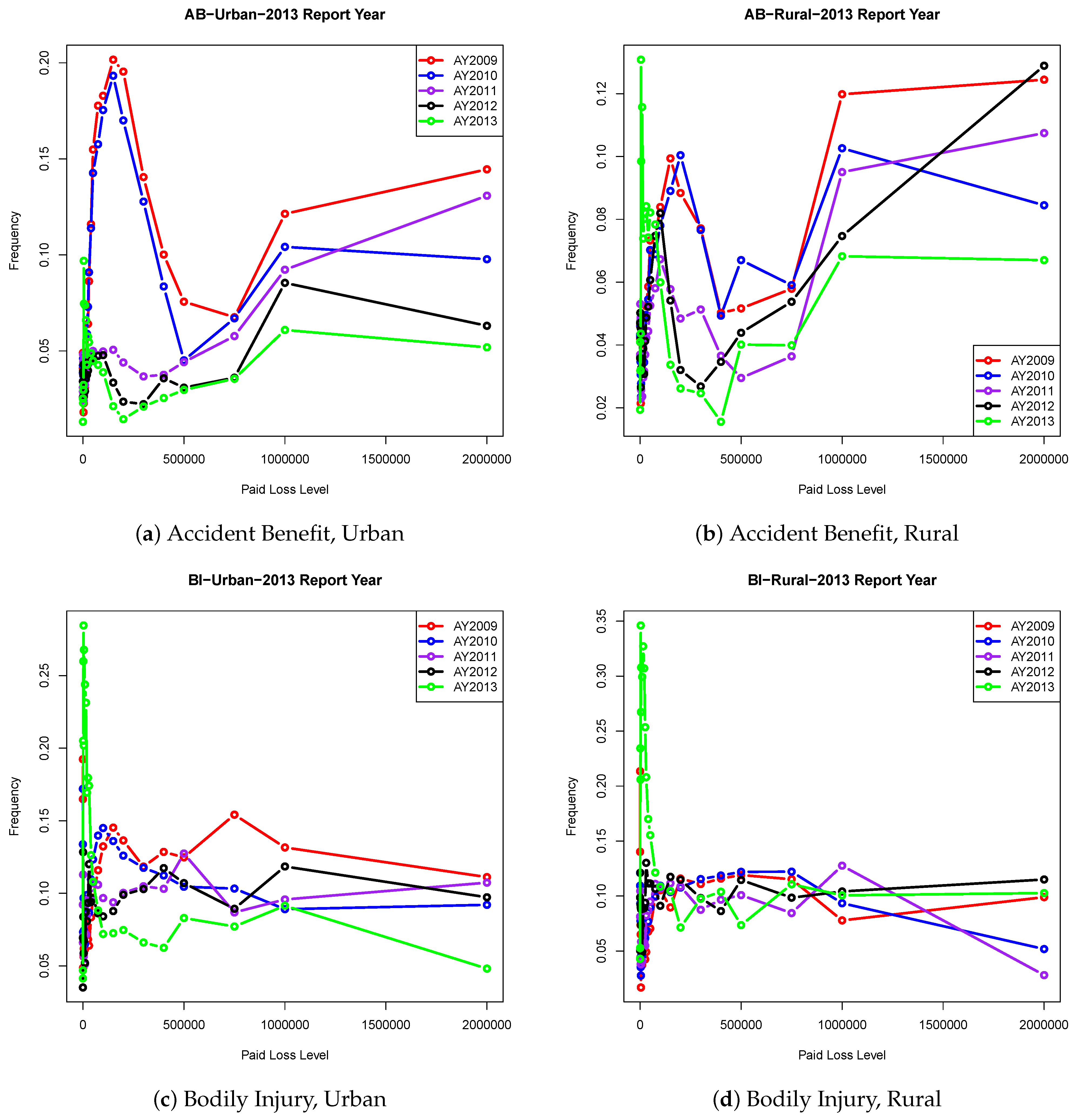
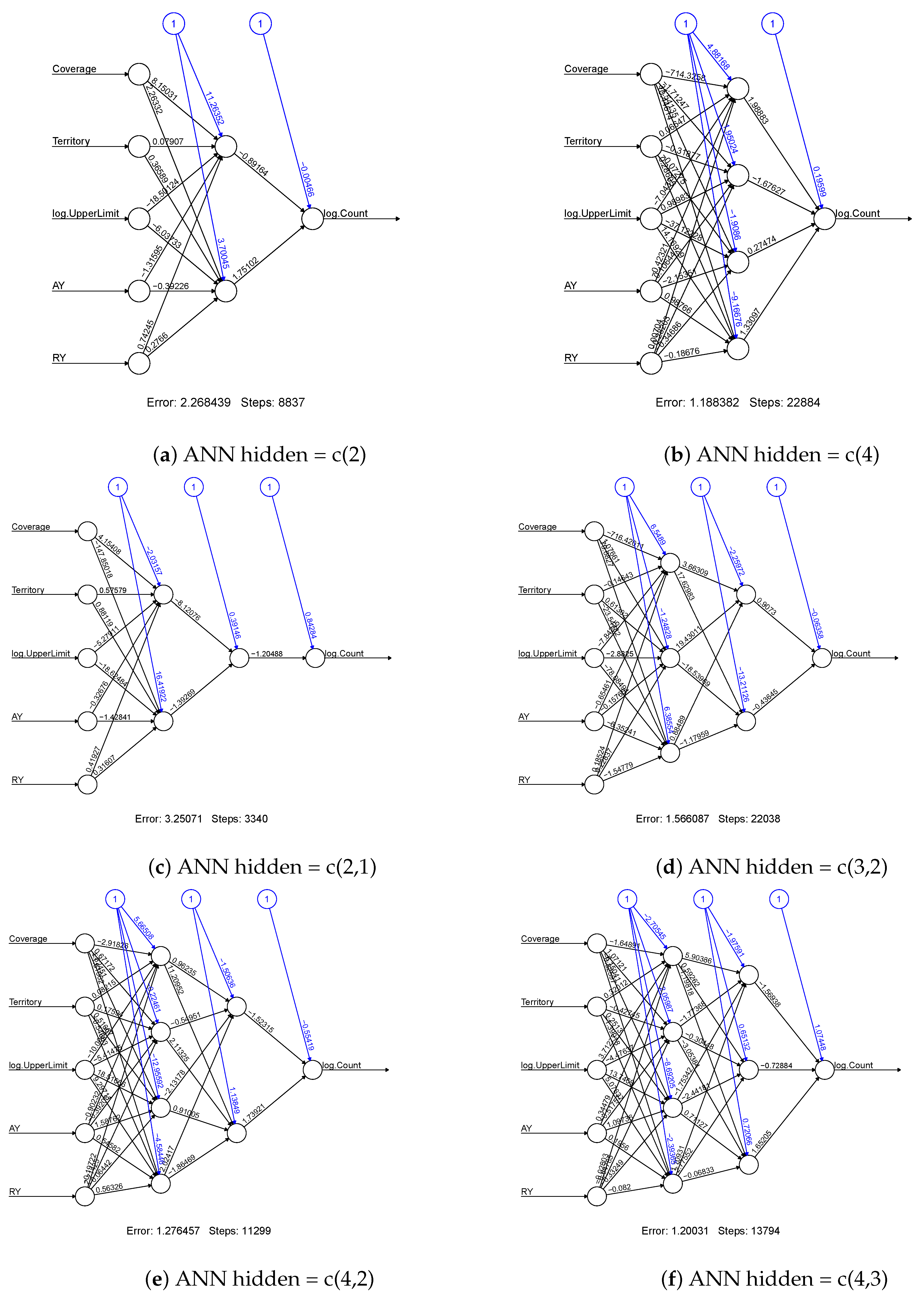
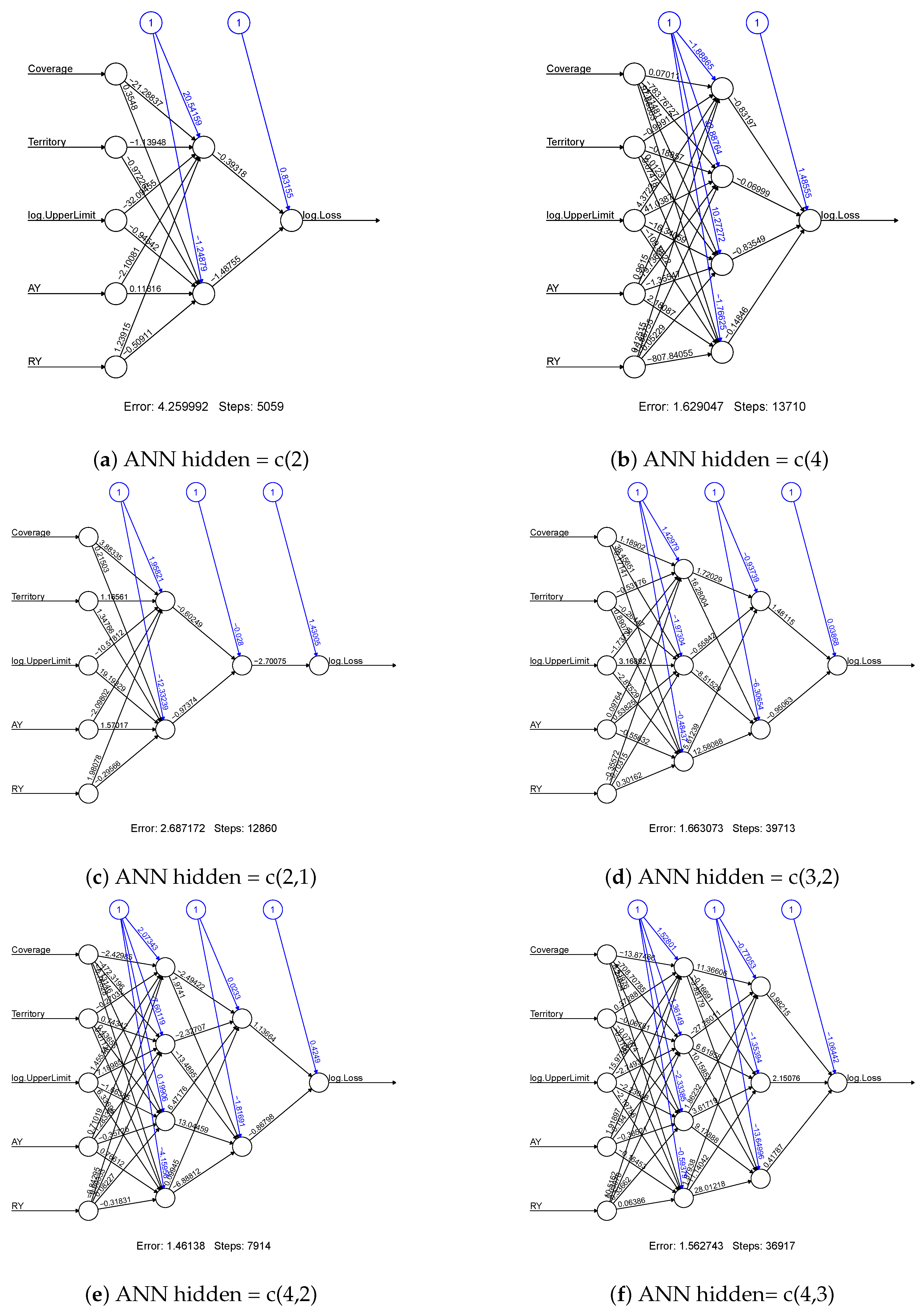
To know more about the Size-of-Loss data distributional behaviour, we present the frequency distribution in Figure 1. The distributions in all types appear to be heavy-tailed, with AB frequency distributions being very extreme. Also, the frequency distributions for AB type seem to have more modes than the data distribution for BI. Within the same coverages, the distributions behave similarly for both Urban and Rural. To see which ANN is more suitable for our data, we first study the network architectures. We consider various combinations of the number of hidden layers and the number of the hidden unit. We consider the cases with one and two hidden layers only. The further increase in the neural network complexity is not recommended due to the constraint of the model stability requirement. Figure 2 displays the network architectures that use the claim counts as the output variable, while Figure 3 presents the ones associated with claim amounts. For each connection within the network, the obtained weight values are displayed. These weight values are used to evaluate the variable importance, which will be discussed later. The blue colour connections are referred to as the weight values of the networks’ bias term, and they are similar to the intercept term in a linear regression model.

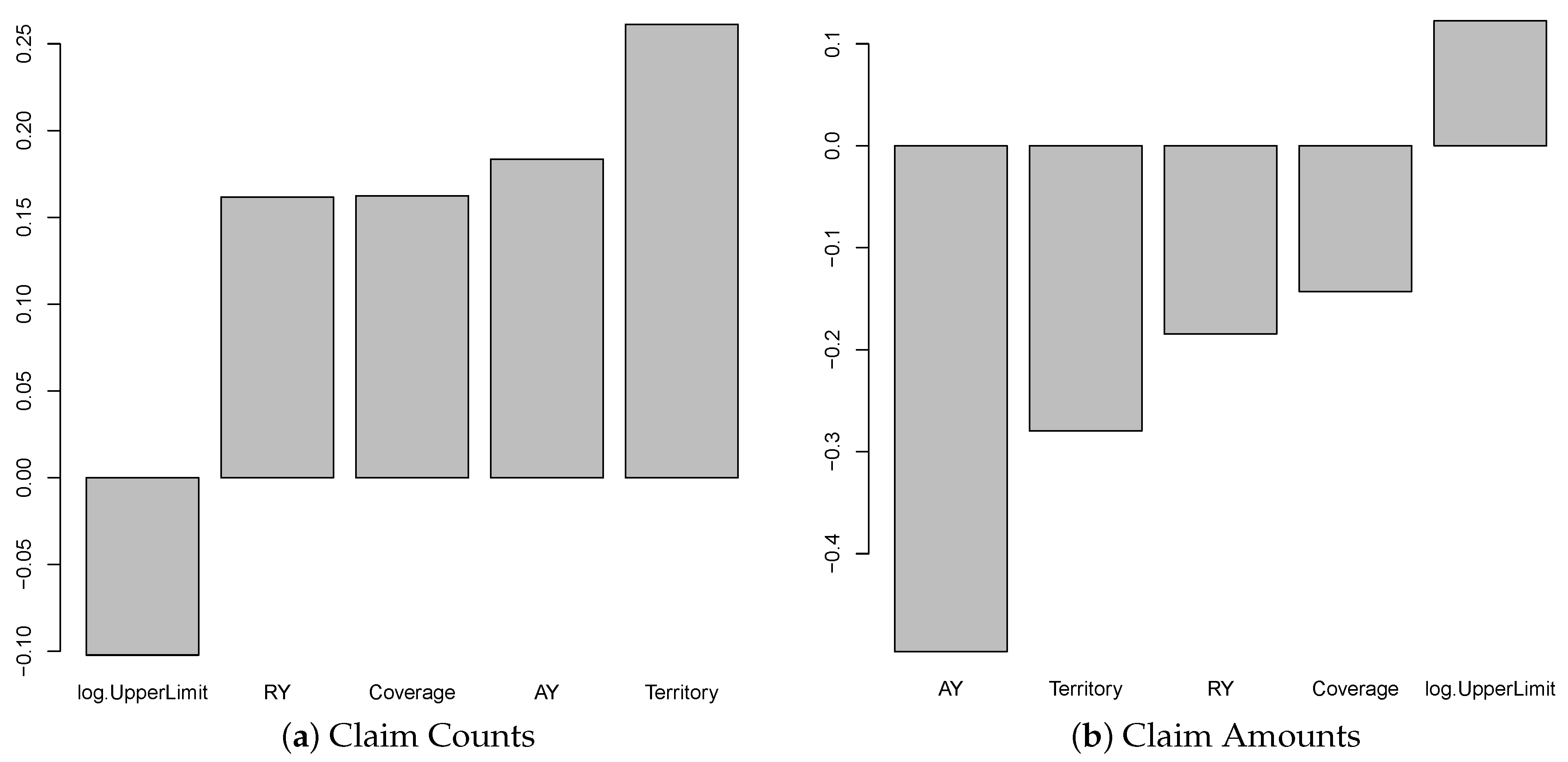
As we can see from the (a) of Figure 2 and Figure 3, the variables of coverage and log. UpperLimit have considerably higher weight values than other input variables. This simplest ANN model gives us some degree of model explainability in terms of the input variables’ contribution through the weight values. However, this simplest model leads to a higher sum of squared errors, which may not be acceptable in terms of model fitting accuracy. When the model complexity is increased, it becomes difficult to observe the variable importance by looking at the weight values. This is why we consider how to improve the model explainability in this work. On the other hand, as shown by the sum of squared errors for the models, the model has four hidden units in the first hidden layer, and three hidden units in the second layer (denoted by ANN-c(4,3)) outperform others. However, ANN-c(4,3) has the highest model complexity that leads to the poorest explainability. According to our experiments, model fitting results are easily affected by initial values, so model stability is low for a high complexity model. However, the model with a lower network complexity, i.e., the network with a single hidden layer and four units within the layer (denoted by ANN-c(4)) seems to be a better choice from both the sum of squared error and network stability perspectives. After identifying the suitable models for modelling claim counts and claim amounts, we then measure the variable importance using the fitted model’s weight values. In this focus, we use the Garson algorithm and Olden function to compute variable importance measures for the selected model (i.e., ANN-c(4)). Figure 4 shows the results by the Garson algorithm, while Figure 5 presents the ones by Olden function. These results are obtained by running the ANN-c(4) model fitting for the given data independently, repeatedly, for 100 times, and the average measures of variable importance are computed for each risk factor. This re-sampling approach aims to minimize both the bias of the estimate and the uncertainty caused by different network architectures and the networks’ initial values.

Figure 4 shows that the results using the Garson algorithm for claim counts and claim amounts as the response variable are reported. From Figure 4, we observe that Size-of-Loss and coverage are more important than others in contributing to the explanation of the variation of the response variable. This may suggest that, for the model we consider, i.e., ANN-c(4), these two risk factors are essential to both claim counts and claim amounts. The result has coincided with the case of using the average loss per claim count, which will be discussed later. Due to the Garson algorithm, only the magnitude of the weight values is considered, but not the sign of the weight values. We are unable to see if the risk factors contribute to the response variable positively or negatively through the weight values of ANN. However, the obtained results for the models we consider are consistent among all response variables, which essentially suggest that coverage and Size-of-Loss are the driving forces for differentiating the patterns of claim counts and claim amounts. To compare the results using different methods, Figure 5 shows the variable importance measures produced by Olden function, which takes both the sign and the magnitude of weight values into consideration. Interestingly, we observe that Size-of-Loss has a negative effect on the claim counts, while the effect on claim amounts becomes positive. This makes sense because we expect that with the increase of Size-of-Loss, the claims counts are decreased. The positive impact on the claim amount may be due to the significant increasing losses. Another important observation is that territory is the most critical variable that leads to the positive effect on claim counts, while AY is the most dominant variable that leads to the negative impact on claim amounts. Since we label the data from urban as one and the data from rural as zero, the positive effect on claim counts implies that urban areas cause significantly more claim counts than the rural area. For the claim amounts model, AY is the most dominant variable and has a negative effect on claim amounts. This may indicate that the decrease of projected loss amounts for more recent accident year. Since the impact from RY on claim amount is also negative, part of the reduction in the projected claim amount may be due to adjustment of case reserve in the new reporting year.

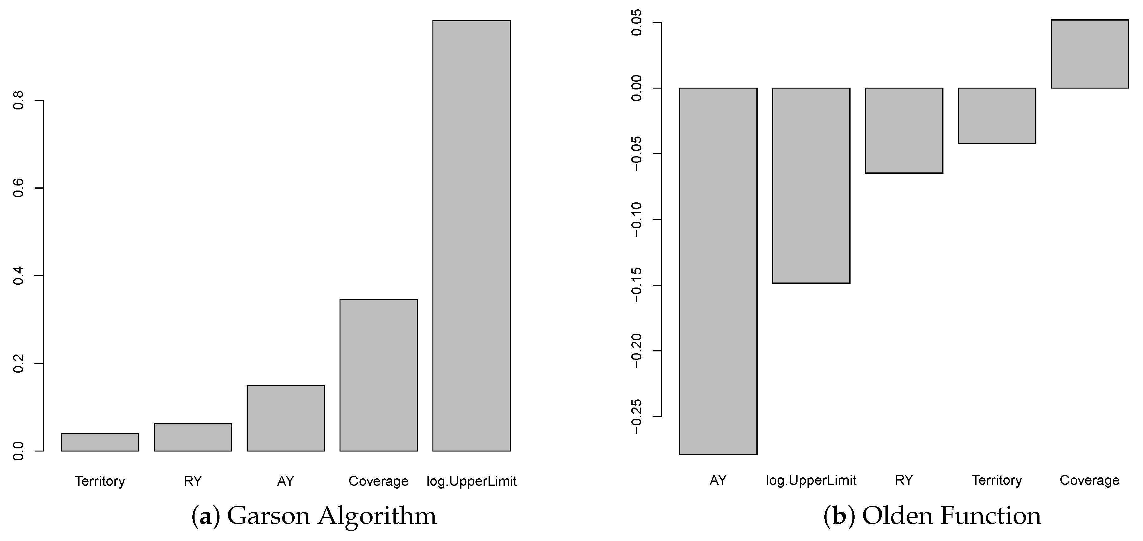
When the claim counts and claim amounts are used to calculate the average loss per claim count, and it is then used as the response variable for the ANN models, the variable importance results behave differently from either claim counts or claim amounts models when the Olden function is used, but the most important variable remains the same. However, this result is consistent with the claim counts and claim amounts models if the Garson algorithm is used. This can be seen from Figure 6, which displays the Garson algorithm and Olden function results, respectively. Moreover, in Figure 6, the Garson algorithm shows that AY is the third most crucial variable, whereas, in the Olden function, AY has the most considerable magnitude of any variable by far. Similarly, the Garson algorithm shows that log.UpperLimit is important, but the Olden function shows a distant second in terms of importance. We should note that the Garson function only works for a single layer network, and the variable importance measure is based on the weight value of this first layer network. However, the Oden function uses the weight values from all hidden layers of the network. Because of this difference in measuring variable importance, we do not expect similar results from these two methods. This is why we observe the different results. Since the Oden function is applied to the multiple layers network and the model performs better than a single layer network, we believe that the results are considered more credible than the results of the Garson function.

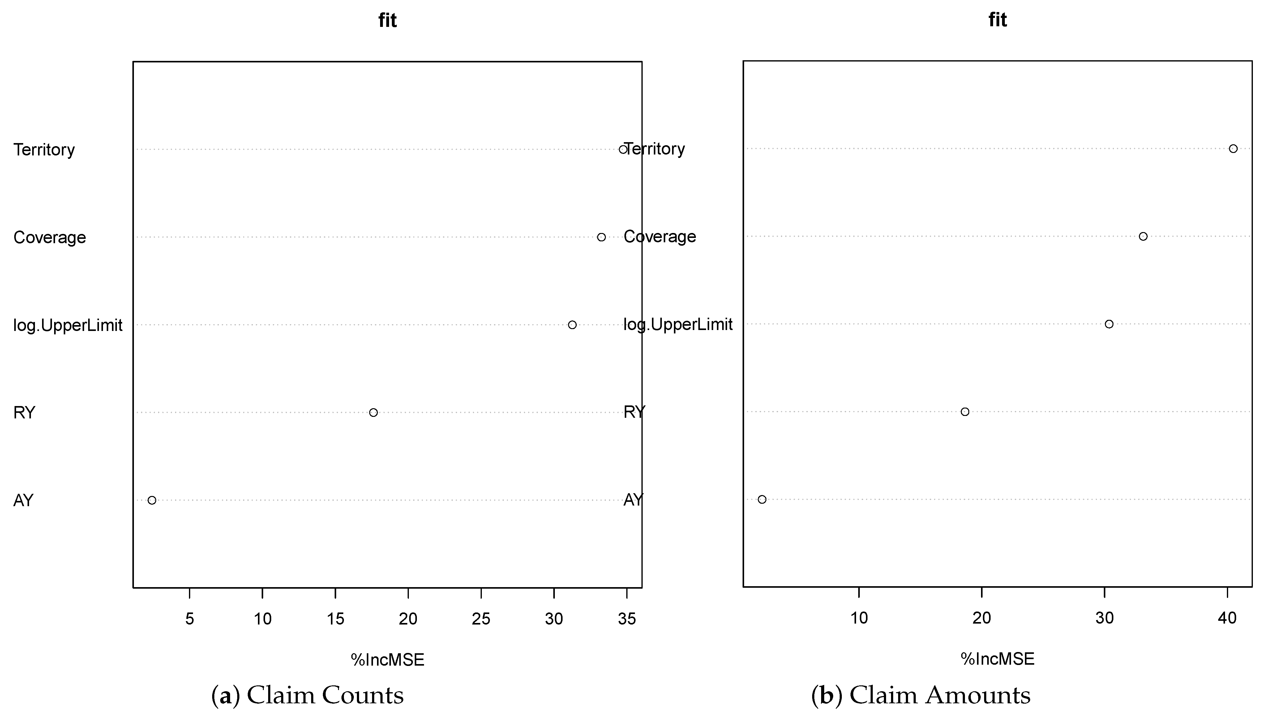
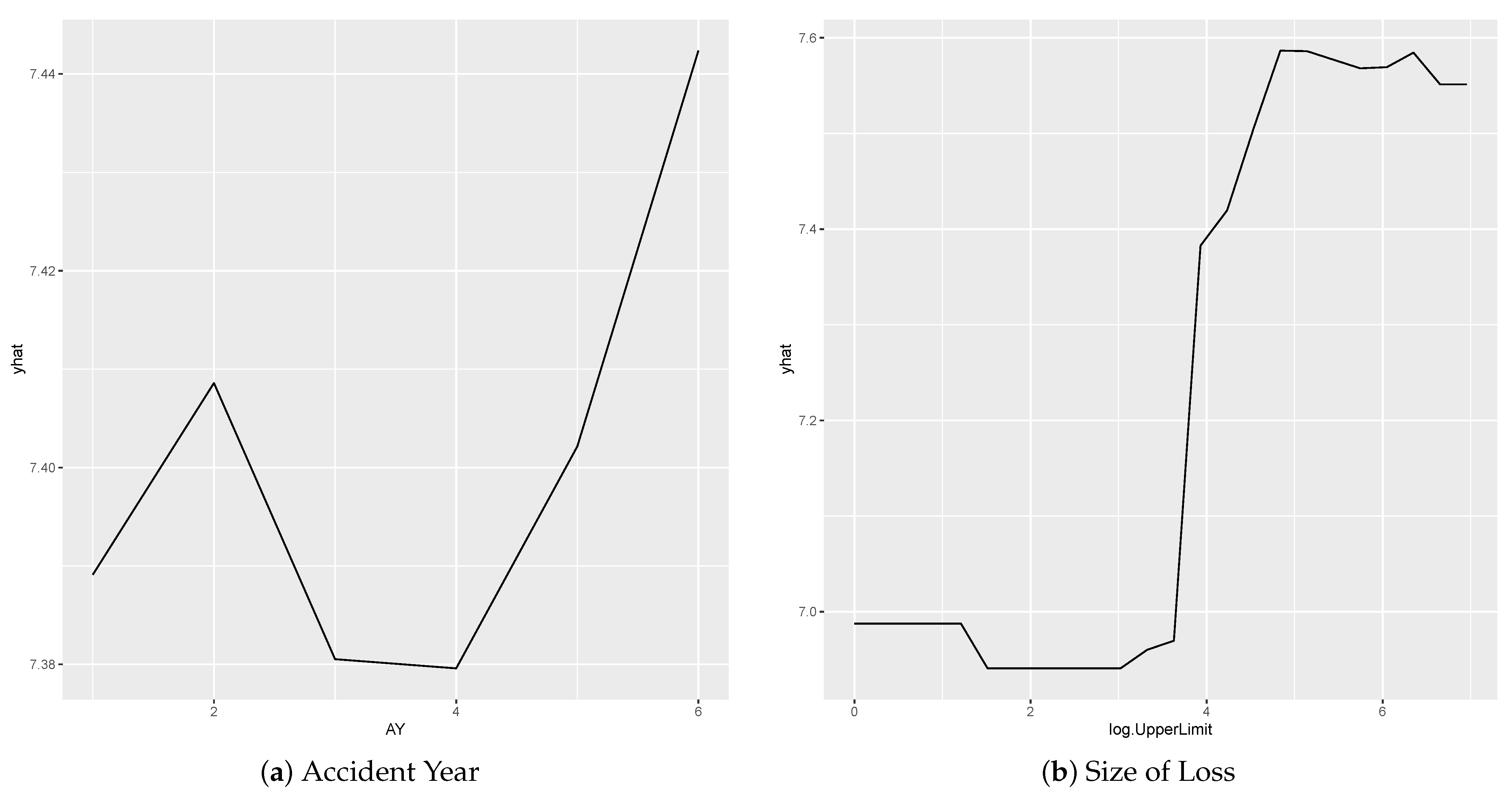
In this work, we compare the Garson function results to the feature importance measures obtained using the random forest model to train a model, which is displayed in Figure 7. We observe that these two approaches behave similarly in identifying the importance of the input variables. Still, the results corresponding to the Garson function are more distinguished. The Garson function suggests that log.UpperLimit variable is the most influential, while the Territory variable is the most important feature by the feature importance method. Since Garson’s variable importance measures are more distinguishable, we conclude that the Garson function results are more appealing than the feature importance measures. We also present the partial dependence plots for both AY and log.UpperLimit as an example, which is displayed in Figure 8. These partial dependence plots were obtained using the random forest method to train a model for making predictions of claim amounts. We observe that the predicted values of claim amounts are quite sensitive to these two variables. Within our approaches, the variable importance for log.UpperLimit is picked up well by the Garson method, while the importance of the AY variable was achieved by using the Olden function for the multiple-layer ANN model.

To better understand how the variable importance measures are affected by different ANN models, we estimate the sample means of variable importance and sampling errors. The results are displayed in

Table 2. The sample mean and the sampling error of variable importance measured by normalized Olden function for the average loss per claim as an input for various ANN models. The first row of the table indicates the structure of hidden layer; for instance, 2 means one hidden layer with two hidden units, and c(2,1) means two hidden layers with two units in the first and one unit in the second layer.

Hidden	c(2)		c(4)		c(2,1)		c(3,2)		c(4,2)		c(4,3)
	Mean	Std	Mean	Std	Mean	Std	Mean	Std	Mean	Std	Mean	Std
Coverage	−0.82	0.06	−0.01	0.09	−0.94	0.03	−0.74	0.06	−0.59	0.07	−0.50	0.08
Territory	−0.35	0.06	−0.12	0.08	−0.75	0.04	−0.33	0.07	−0.36	0.07	−0.23	0.08
Size-of-Loss	+0.82	0.06	−0.02	0.09	+0.94	0.03	+0.70	0.07	+0.58	0.08	+0.38	0.09
AY	−0.65	0.05	−0.40	0.08	−0.79	0.03	−0.47	0.06	−0.53	0.07	−0.36	0.08
RY	−0.40	0.06	−0.12	0.08	−0.75	0.04	−0.35	0.07	−0.34	0.08	−0.26	0.08

,

Table 3. The sample mean and the sampling error of variable importance measured by normalized Olden function for the claim counts as an input for various ANN models. The first row of the table indicates the structure of hidden layer; for instance, 2 means one hidden layer with two hidden units and c(2,1) means two hidden layers with two units in the first and one unit in the second layer.

Hidden	c(2)		c(4)		c(2,1)		c(3,2)		c(4,2)		c(4,3)
	Mean	Std	Mean	Std	Mean	Std	Mean	Std	Mean	Std	Mean	Std
Coverage	0.44	0.08	0.26	0.09	0.40	0.08	0.40	0.08	0.37	0.08	0.30	0.09
Territory	0.63	0.06	0.30	0.07	0.83	0.04	0.43	0.07	0.40	0.07	0.22	0.08
Size-of-Loss	−0.49	0.09	−0.29	0.09	−0.58	0.09	−0.43	0.07	−0.50	0.08	−0.40	0.09
AY	0.45	0.05	0.13	0.07	0.59	0.05	0.26	0.06	0.21	0.06	0.03	0.07
RY	0.56	0.07	0.10	0.08	0.74	0.05	0.35	0.07	0.33	0.07	0.11	0.07

and

Table 4. The sample mean and the sampling error of variable importance measured by normalized Olden function for the claim amounts as an input for various ANN models. The first row of the table indicates the structure of hidden layer; for instance, 2 means one hidden layer with two hidden units and c(2,1) means two hidden layers with two units in the first and one unit in the second layer.

Hidden	c(2)		c(4)		c(2,1)		c(3,2)		c(4,2)		c(4,3)
	Mean	Std	Mean	Std	Mean	Std	Mean	Std	Mean	Std	Mean	Std
Coverage	−0.52	0.05	0.10	0.09	−0.05	0.08	0.36	0.08	0.27	0.09	0.20	0.09
Territory	−0.79	0.02	−0.38	0.08	−0.76	0.04	−0.52	0.07	−0.32	0.08	−0.13	0.08
Size-of-Loss	0.95	0.02	−0.00	0.09	0.40	0.08	−0.12	0.09	−0.26	0.09	−0.17	0.09
AY	−0.88	0.03	−0.61	0.07	−0.90	0.03	−0.68	0.06	−0.56	0.06	−0.29	0.07
RY	−0.92	0.03	−0.45	0.08	−0.93	0.03	−0.60	0.07	−0.41	0.08	−0.21	0.08

, and they were calculated using the normalized Olden function. Different models lead to different estimates of the variable importance. The experimental results shown in all these tables may suggest the difficulty of interpreting the results when different models are considered. Therefore, it is critical to identify a most reliable model and make inferences by conditioning on the assumption that the selected model is the true model. With this in mind, we compare the variable importance measures for major risk factors under the best ANN architecture, and these results are presented in

Table 5. The comparison of average variable importance measured by normalized Olden function based on the best ANN architecture, respectively for the claim count, claim amounts and average loss per claim as an input.

	Average Loss Per Claim	Claim Count	Claim Amount
Coverage	−0.50	+0.30	+0.27
Territory	−0.23	+0.22	−0.32
Size-of-Loss	+0.38	−0.40	−0.26
AY	−0.36	+0.03	−0.56
RY	−0.26	+0.11	−0.41

. Overall, the variable importance measures all appear to be large and not very different, except for the case of the claim count as the input, in which the importance measure of AY is smaller than other variables.

Finally, to see the performance of the model that we chose, we display the plots of predicted values versus actual output values in Figure 9, for both cases of the claim amount and average loss per claim as response variables. From the result, we can see that the ANN-c(4) with the average loss per claim count outperforms the ANN-c(4) with the claim amount. This result was also compared to GLM results, where the selected one are reported in Figure 9, and we found that ANN-c(4) outperforms the GLM.

5. Discussion

In the context of interpretable machine learning, interpretable models have been widely used. In actuarial science, linear models (LM), GLM, and GAM are popular modelling tools in auto insurance pricing to obtain risk relativities (Ohlsson and Johansson 2010; Xie and Lawniczak 2018). A linear model is a suitable choice when variables appear to be linearly related to the model response variable; it does not work well for the situation where interaction among variables or non-linear relationships are found. GLM overcomes the limitation of multiple linear regression models, where the normality and constant variance are often assumed. By extending the error probability distribution from a normal distribution to an exponential family (Dobson and Barnett 2008), GLM enables a line of choices for the error distribution. It also allows one to specify the functionality between the variance of the response variable and the mean response so that the model can capture the extra dispersion caused by the data. However, in the context of measuring the importance of risk factors, GLM has certain limitations. In auto insurance rate-making, many independent variables or risk factors are categorical types. The independent variables within the GLM are designed as dummy variables based on the levels of categorical variables. Measuring the importance of the variable within GLM can be done easily for each factor level but not for the whole factor itself. The model captures the contribution of different combinations of the levels among the factors considered. Unlike ANN, the input variables are the factors with various levels, and the weight values are obtained for each input variable. It is possible to derive the variable importance for a numeric variable in GLM by calculating the t-test statistics for the coefficients or obtaining the p-value of the statistical test. When the GLM contains categorical variables, an F-test may be used to address the significance of the contribution of the variables, but it is difficult to measure the importance using the F-statistics. This is because the F test is quite sensitive to the violation of normality, which is often the case when dealing with loss distribution. Therefore, it requires further consideration of some suitable approaches to derive the importance measures of each underlying categorical variable when using GLM for pricing, but this is out of the scope of this paper. The use of ANN enables us to measure the variable importance directly, no matter the type of the input variables. It does not require the error distribution assumption or running statistical tests, which may be sensitive to the assumption on the sampling distribution. These are considered another advantage for ANN when comparing with other predictive modelling techniques. Furthermore, our empirical study shows that ANN outperforms the GLM when modelling the size of loss data. The mean square errors of the model residuals are much smaller than the GLM approach. The residuals of ANN model are much more homogeneous than the ones from GLM models. Evaluating ANN with the study of variable importance measure leads to a better understanding of risk factors’ effects to make more informed decisions in rate-making or rate regulation. When this is the case, insurance regulators are more comfortable in judging the appropriateness of risk relativity in rate fillings conducted by insurance companies.

According to the recent survey of Kagglers in terms of choice for machine learning tools, R has been a preferred tool for Business Analyst, Data Analyst, Data Miner, Predictive Modeller, and Statistician, who are often involved in insurance rate making. Due to this work’s nature, we adopt R and its package, called "neuralnet", to implement our study results. The main reason for making this choice is that it has been widely used for machine learning applications. It is an excellent tool for graphical representation of the model with the weights on each connection in neural network models, particularly for a small number of input variables, like in our case. This package uses backpropagation for parameter calibration and allows flexible settings through custom-choice of error and activation function.

6. Conclusions and Future Work

A single metric such as prediction accuracy is an incomplete description of most real-world tasks in predictive modelling. The need for model interpretability is due to incompleteness in a given problem formulation. It is not enough to get higher prediction accuracy; it is also necessary to know how the model accurately predicts. There is no explicit mathematical definition of model interpretability or data explainability. A non-mathematical description is of how much a model user can understand the cause of the decisions in the decision marking or how consistently a learned model can predict an accurate result. Our work belongs to the first type. It aims at providing some guidance on what advanced rate-making methodologies are suitable for facilitating the rate-filing review process. From the insurance regulator’s point of view, it is critical to know the insights of methods used for rate-making and the potential impact of risk factors and the mathematical model used to conduct the analysis. This makes the justification of any decision made more accessible and transparent to management responsible for a higher level of impact from regulatory policies, particularly the determination of reform and significant change of maximum coverage levels of insurance losses. On the other hand, the insurance loss data explainability improvement can help stakeholders better understand the nature of data patterns and the relationship between risk factors and the loss level metrics, such as loss counts, loss amounts, and loss costs. Therefore, decision-makers can make better policies or regulations that fit real-world situations, and communication between the insurance companies and regulatory authorities will become smoother and more effective.

In this work, the modelling problems of how claim counts, claim amounts, and average loss per claim are related to major risk factors in auto insurance rate regulation were considered. The major risk factors include accident year, reporting year, territory, coverage, and Size-of-Loss. Artificial neural network models were applied within the problem, and variable importance measures were introduced to improve the model explainability. The obtained results from different approaches of using weight values of ANN to measure the variable importance were compared, and the most dominant risk factors were identified. Through the study, we found that the variable importance measures by the Garson algorithm or Olden function can help identify the critical variables that contribute to explaining the variation of the response variable in ANN models. The obtained results were not necessarily consistent, since the variable importance measures make use of the different sources of information from the fitted model. However, our study shows that both Size-of-Loss and coverage are two crucial factors for claim counts, claim amounts, and average loss per claim. This finding is based on the selected low-complexity ANN model, in which the Garson algorithm is applicable.

Due to the complexity and lack of model explainability, neural network models have not yet been used in auto insurance rate regulation. This work illustrates the applicability of using a small-scale network architecture for modelling the claim frequency or claim severity by balancing the model complexity and its explainability. This work demonstrates the usefulness of proposed insurance rate regulation methods, particularly from the rate-filing perspectives. Although this study focuses on analyzing major risks only, the proposed method can be applied to more general insurance pricing problems. Therefore, insurance companies may use ANN models to predict future claim losses or future claim counts by pricing groups or individuals. That is to say, this work can be extended to the case when we have many observed zeroes in the response variable. However, in this case, the logarithm transformation on the loss cost to improve model variance homogeneity is not applicable. Another key aspect of using neural networks is the choice of network architecture. This is similar to other predictive modelling approaches, which aim for the optimal model via some cross-validation to evaluate the model error and select the suitable model based on the minimum cross-validated model error. Improving model explainability was our focus. Therefore, it is not recommended to apply a large-scale network architecture unless the model is interpretable. Our approach searches ofr the optimal network architecture within a designed search space, and this idea can be generalized to risk-factor study using individual claim loss. From this study, we have seen that the Size-of-Loss is a significant risk factor. In the future, further investigation of this factor may be needed to better understand the uncertainty behind the data observation and the relationship between Size-of-Loss and other statistical measures of loss, such as loss frequency. Our future work will focus on estimating Size-of-Loss probability distribution using multivariate statistical approaches such as functional principal component analysis and finite mixture models.

References

- Adadi, Amina, and Mohammed Berrada. 2018. Peeking inside the black-box: A survey on Explainable Artificial Intelligence (XAI). IEEE Access 6: 52138–60. [Google Scholar] [CrossRef]
- Arrieta, Alejandro Barredo, Natalia Díaz-Rodríguez, Javier Del Ser, Adrien Bennetot, Siham Tabik, Alberto Barbado, Salvador García, Sergio Gil-Lopez, Daniel Molina, Richard Benjamins, and et al. 2020. Explainable Artificial Intelligence (XAI): Concepts, taxonomies, opportunities and challenges toward responsible AI. Information Fusion 58: 82–115. [Google Scholar] [CrossRef] [Green Version]
- Asmussen, Søren, and Reuven Y. Rubinstein. 1999. Sensitivity analysis of insurance risk models via simulation. Management Science 45: 1125–41. [Google Scholar] [CrossRef]
- Ayuso, Mercedes, Montserrat Guillen, and Jens Perch Nielsen. 2019. Improving automobile insurance ratemaking using telematics: Incorporating mileage and driver behaviour data. Transportation 46: 735–52. [Google Scholar] [CrossRef] [Green Version]
- Beaudouin, Valérie, Isabelle Bloch, David Bounie, Stéphan Clémençon, Florence d’Alché-Buc, James Eagan, Winston Maxwell, Pavlo Mozharovskyi, and Jayneel Parekh. 2020. Flexible and Context-Specific AI Explainability: A Multidisciplinary Approach. arXiv arXiv:2003.07703. [Google Scholar] [CrossRef] [Green Version]
- Bhowmik, Rekha. 2011. Detecting auto insurance fraud by data mining techniques. Journal of Emerging Trends in Computing and Information Sciences 2: 156–62. [Google Scholar]
- Bishop, Christopher M. 2006. Pattern Recognition and Machine Learning. New York: Springer. [Google Scholar]
- Dionne, Georges, Christian Gouriéroux, and Charles Vanasse. 1999. Evidence of adverse selection in automobile insurance markets. In Automobile Insurance: Road safety, New Drivers, Risks, Insurance Fraud and Regulation. Boston: Springer, pp. 13–46. [Google Scholar]
- Dobson, Annette J., and Adrian G. Barnett. 2008. An Introduction to Generalized Linear Models. Boca Raton: CRC Press. [Google Scholar]
- Došilović, Filip Karlo, Mario Brčić, and Nikica Hlupić. 2018. Explainable artificial intelligence: A survey. Paper presented at 2018 41st International Convention on Information and Communication Technology, Electronics and Microelectronics (MIPRO), Opatija, Croatia, May 21–25; pp. 210–15. [Google Scholar]
- Dugas, Charles, Yoshua Bengio, Nicolas Chapados, Pascal Vincent, Germain Denoncourt, and Christian Fournier. 2003. Statistical learning algorithms applied to automobile insurance ratemaking. In CAS Forum. Arlington: Casualty Actuarial Society, vol. 1, pp. 179–214. [Google Scholar]
- Farbmacher, Helmut, Leander Löw, and Martin Spindler. 2019. An Explainable Attention Network for Fraud Detection in Claims Management. Journal of Econometrics. [Google Scholar]
- Fialova, Vendula, and Andrea Folvarcna. 2020. Default Prediction Using Neural Networks for Enterprises from the Post-Soviet Country. Ekonomicko-Manazerske Spektrum 14: 43–51. [Google Scholar] [CrossRef]
- Fisher, Aaron, Cynthia Rudin, and Francesca Dominici. 2019. All Models are Wrong, but Many are Useful: Learning a Variable’s Importance by Studying an Entire Class of Prediction Models Simultaneously. Journal of Machine Learning Research 20: 1–81. [Google Scholar]
- Frees, Edward W. 1998. Relative importance of risk sources in insurance systems. North American Actuarial Journal 2: 34–49. [Google Scholar] [CrossRef]
- Friedman, Jerome H. 2001. Greedy function approximation: A gradient boosting machine. Annals of Statistics 29: 1189–232. [Google Scholar] [CrossRef]
- Fürst, Elmar, Peter Oberhofer, Christian Vogelauer, Rudolf Bauer, and David M. Herold. 2019. Innovative methods in European road freight transport statistics: A pilot study. Journal of Statistics and Management Systems 22: 1445–66. [Google Scholar] [CrossRef] [Green Version]
- Gao, Guangyuan, and Mario V. Wüthrich. 2018. Feature extraction from telematics car driving heatmaps. European Actuarial Journal 8: 383–406. [Google Scholar] [CrossRef]
- Garson, David G. 1991. Interpreting neural network connection weights. AI Expert 6: 47–53. [Google Scholar]
- Gevrey, Muriel, Ioannis Dimopoulos, and Sovan Lek. 2003. Review and comparison of methods to study the contribution of variables in artificial neural network models. Ecological Modelling 160: 249–64. [Google Scholar] [CrossRef]
- Gilenko, Evgenii V., and Elena A. Mironova. 2017. Modern claim frequency and claim severity models: An application to the Russian motor own damage insurance market. Cogent Economics & Finance 5: 1311097. [Google Scholar]
- Henckaerts, Roel, Marie-Pier Côté, Katrien Antonio, and Roel Verbelen. 2020. Boosting insights in insurance tariff plans with tree-based machine learning methods. North American Actuarial Journal 25: 1–31. [Google Scholar] [CrossRef]
- Hsiao, Cheng, Changseob Kim, and Grant Taylor. 1990. A statistical perspective on insurance rate-making. Journal of Econometrics 44: 5–24. [Google Scholar] [CrossRef]
- İşeri, Ali, and Bekir Karlık. 2009. An artificial neural networks approach on automobile pricing. Expert Systems with Applications 36: 2155–60. [Google Scholar] [CrossRef]
- Kim, Jinkyu, and John Canny. 2018. Explainable Deep Driving by Visualizing Causal Attention. In Explainable and Interpretable Models in Computer Vision and Machine Learning. Cham: Springer, pp. 173–93. [Google Scholar]
- Kliestik, Tomas, Maria Misankova, Katarina Valaskova, and Lucia Svabova. 2018. Bankruptcy prevention: New effort to reflect on legal and social changes. Science and Engineering Ethics 24: 791–803. [Google Scholar] [CrossRef] [PubMed]
- Kovacova, Maria, Tomas Kliestik, Katarina Valaskova, Pavol Durana, and Zuzana Juhaszova. 2019. Systematic review of variables applied in bankruptcy prediction models of Visegrad group countries. Oeconomia Copernicana 10: 743–72. [Google Scholar] [CrossRef] [Green Version]
- Lu, Xiaowei, Fu Jiang, and Liwen Hou. 2005. Customer features extraction based on customer ontology. Computer Engineering 31: 31–33. [Google Scholar]
- Maitra, Saikat, and Jun Yan. 2008. Principle component analysis and partial least squares: Two dimension reduction techniques for regression. Applying Multivariate Statistical Models 79: 79–90. [Google Scholar]
- McClenahan, Charles L. 2014. Ratemaking. Wiley StatsRef: Statistics Reference Online, Wiley Online Library. [Google Scholar]
- Ohlsson, Esbjörn, and Björn Johansson. 2010. Non-Life Insurance Pricing with Generalized Linear Models. Berlin: Springer, vol. 2. [Google Scholar]
- Olden, Julian D., and Donald A. Jackson. 2002. Illuminating the “black box”: A randomization approach for understanding variable contributions in artificial neural networks. Ecological Modelling 154: 135–50. [Google Scholar] [CrossRef]
- Olden, Julian D., Michael K. Joy, and Russell G. Death. 2004. An accurate comparison of methods for quantifying variable importance in artificial neural networks using simulated data. Ecological Modelling 178: 389–97. [Google Scholar] [CrossRef]
- Parodi, Pietro. 2012. Computational intelligence with applications to general insurance: A review: I—The role of statistical learning. Annals of Actuarial Science 6: 307–43. [Google Scholar] [CrossRef]
- Ribeiro, Bernardete, Armando Vieira, and Joao Carvalho das Neves. 2006. Sparse bayesian models: Bankruptcy-predictors of choice? Paper presented at 2006 IEEE International Joint Conference on Neural Network Proceedings, Vancouver, BC, Canada, July 16–21; pp. 3377–81. [Google Scholar]
- Samek, Wojciech, Thomas Wiegand, and Klaus-Robert Müller. 2017. Explainable artificial intelligence: Understanding, visualizing and interpreting deep learning models. arXiv arXiv:1708.08296. [Google Scholar]
- Sundararajan, Mukund, and Amir Najmi. 2019. The many Shapley values for model explanation. arXiv arXiv:1908.08474. [Google Scholar]
- Sun, Ning, Hongxi Bai, Yuxia Geng, and Huizhu Shi. 2017. Price evaluation model in second-hand car system based on BP neural network theory. Paper presented at 2017 18th IEEE/ACIS International Conference on Software Engineering, Artificial Intelligence, Networking and Parallel/Distributed Computing (SNPD), Kanazawa, Japan, June 26–28; pp. 431–36. [Google Scholar]
- Verbelen, Roel, Katrien Antonio, and Gerda Claeskens. 2018. Unravelling the predictive power of telematics data in car insurance pricing. Journal of the Royal Statistical Society: Series C (Applied Statistics) 67: 1275–304. [Google Scholar] [CrossRef] [Green Version]
- Wüthrich, Mario V. 2019. Bias regularization in neural network models for general insurance pricing. European Actuarial Journal 10: 179–202. [Google Scholar] [CrossRef]
- Xie, Shengkun, and Anna T. Lawniczak. 2018. Estimating Major Risk Factor Relativities in Rate Filings Using Generalized Linear Models. International Journal of Financial Studies 6: 84. [Google Scholar] [CrossRef] [Green Version]
- Xie, Shengkun. 2019. Defining Geographical Rating Territories in Auto Insurance Regulation by Spatially Constrained Clustering. Risks 7: 42. [Google Scholar] [CrossRef] [Green Version]
- Xie, Shengkun, and Clare Chua-Chow. 2020. Improving Statistical Reporting Data Explainability via Principal Component Analysis. In Proceedings of the 9th International Conference on Data Science, Technology and Applications, DATA, online streaming. Setúbal: Setúbal: SciTePress, pp. 185–92. [Google Scholar]
- Yan, Jun, James Guszcza, Matthew Flynn, and Cheng-Sheng Peter Wu. 2009. Applications of the offset in property-casualty predictive modeling. In Casualty Actuarial Society E-Forum. Arlington: Casualty Actuarial Society, p. 366. [Google Scholar]
- Yeo, Ai Cheo, Kate A. Smith, Robert J. Willis, and Malcolm Brooks. 2001. Modeling the effect of premium changes on motor insurance customer retention rates using neural networks. In International Conference on Computational Science. Berlin/Heidelberg: Springer, pp. 390–99. [Google Scholar]
- Yunos, Zuriahati Mohd, Aida Ali, Siti Mariyam Shamsyuddin, and Noriszura Ismail. 2016. Predictive Modelling for Motor Insurance Claims Using Artificial Neural Networks. International Journal of Advances in Soft Computing and Its Applications 8: 160–72. [Google Scholar]
Figure 1.
The Size-of-Loss patterns of different accident years and different combinations of coverage and territory for the 2013 reporting year.
Figure 2.
The ANN models with different hidden layer and hidden units, for the input variables of reporting year, accident year, log-scale upper limit of Size-of-Loss intervals, territory and coverage, respectively, and the output variable of claim counts. The obtained model errors for each network architecture are cross-validated errors.
Figure 3.
The ANN models with different hidden layer and hidden units, for the input variables of reporting year, accident year, log-scale upper limit of Size-of-Loss intervals, territory and coverage, respectively, and the output variable of claim amount. The obtained model errors for each network architecture are cross-validated errors.
Figure 4.
The variable importance measures by Garson algorithm for three layer ANN models with four hidden units. The results are the mean values of importance measures by 100 runs of ANN model fitting.
Figure 5.
The variable importance measures by Olden function for three layer ANN models with four hidden units. The results are the mean values of importance measures by 100 runs of ANN model fitting.
Figure 6.
The variable importance measures by Garson algorithm and Olden function for three-layer ANN models with four hidden units in the hidden layer and taking the average loss per claim count as the response variable. The results are the mean values of importance measures by 100 runs of ANN model fitting.
Figure 7.
The feature importance measures obtained by fitting the data to the random forest model using claim counts and claim amounts, respectively, as a dependant variable.
Figure 8.
Partial dependence plot for selected variable in the random forest model using claim amount as the model response variable.
Figure 9.
The (a,b) plots are predicted values versus actual for claim amounts and average loss per claim count, respectively, as the response variable for the ANN-c(4). The (c,d) plots are predicted values versus actual claim counts from the GLM models with the Gaussian error function and the Poisson error function, respectively. The (e,f) plots are predicted values versus actual loss cost from the GLM models with the Gaussian error function and the Gamma error function, respectively.