Investigation of the Spatio-Temporal Behaviour of Submarine Groundwater Discharge Using a Low-Cost Multi-Sensor-Platform

Abstract

Submarine groundwater discharge (SGD) is an important pathway of nutrients into coastal areas. During the last decades, interest of researchers in SGDs has grown continuously. However, methods applied for SGD research usually focus on the aquifer or on the mixing processes on larger scales. The distribution of discharged water within the water column is not well investigated. Small remotely operated vehicles (ROV) equipped with environmental sensors can be used to investigate the spatial distribution of environmental parameters in the water column. Herein, a low-cost multi-sensor platform designed to investigate the spatial distribution of water quality properties is presented. The platform is based on an off-the-shelf underwater vehicle carrying various environmental sensors and a short-baseline localisation system. This contribution presents the results of SGD investigations in the area of Woodman Point (Western Australia). Various potential SGD plumes were detected using a skiff equipped with a recreational echo sounder. It was demonstrated that this inexpensive equipment could be used to detect and investigate SGDs in coastal areas. In addition, the low-cost multi-sensor platform was deployed to investigate the spatial distribution of environmental parameters including temperature (T), electric conductivity (EC), dissolved oxygen (DO), oxidation-reduction potential (ORP), pH, and dissolved organic matter fluorescence (FDOM). Three ROV surveys were conducted from different skiff locations. Analyses of the spatial distribution of the environmental parameters allowed the identification of nine potential SGD plumes. At the same locations, plumes were identified during the sonar surveys. In addition, fuzzy logic was used for the fusion of salinity, DO, and FDOM readings in order to enhance SGD detection capability of the designed multi-sensor system. The fuzzy logic approach identified 293 data points as potential within a SGD plume. Average minimum-distance between these points and the identified SGD plumes was 0.5 m and 0.42 m smaller than the minimum-distance average of the remaining data points of survey one and three respectively. It was shown that low-cost ROVs, equipped with environmental sensors, could be an important tool for the investigation of the spatio-temporal behaviour of SGD sites. This method allows continuous mapping of environmental parameters with a high spatial and temporal resolution. However, to obtain deeper insights into the influence of SGDs on the nearshore areas, this method should be combined with other well-established methods for SGD investigation, such as pore water sampling, remote sensing, or groundwater monitoring.

1. Introduction

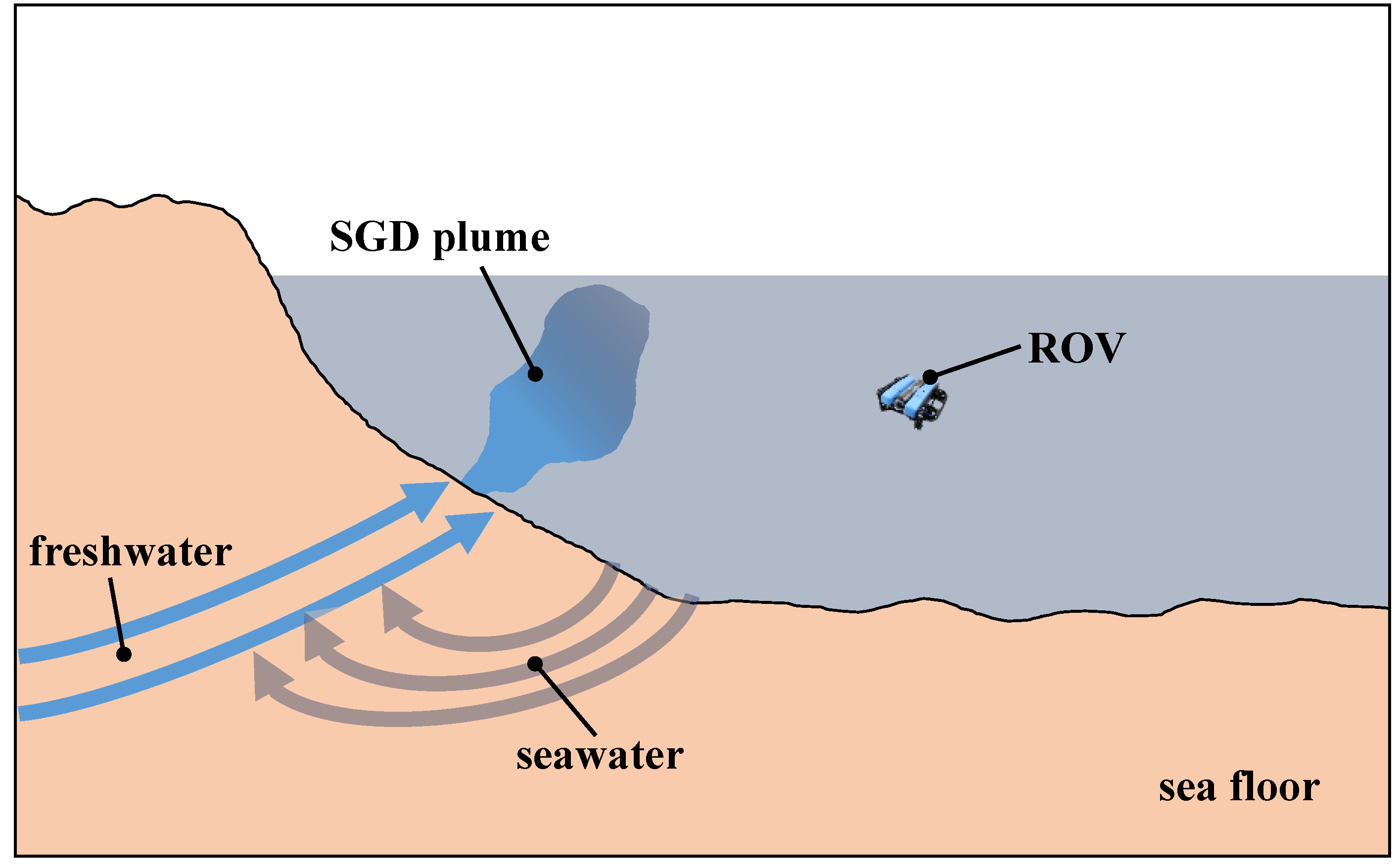
The term Submarine Groundwater Discharge (SGD) covers any flow of water across the seabed into the coastal ocean on continental margins, regardless the composition and the driving force (Figure 1) [1,2]. In general, groundwater can discharge either via submarine springs or via disseminated seepages [1]. Slow, yet persistent seepage of groundwater through sediments will occur at any place where an aquifer with a positive hydraulic head is connected to a surface water body [3].

Surić et al. [5] defined three different kinds of SGD patterns occurring within karstic regions: (1) diffuse seepage through loose sediment, (2) diffuse flow through karst bedrock fissures, and (3) concentrated outflow from conduits and caves. The source type is mainly dependent on the nature of soil, especially on homogeneity and permeability of the soil [6]. While homogeneous soils, such as sand, favour the development of diffuse seepage, inhomogeneous subsoils such as karst [5], limestone or volcanic undergrounds [7] provide for the formation of underwater springs. In these cases, the water flows mainly through cavities in underground streams [6].

In limestone soil, the dissolution of heterogeneous distributed easily soluble minerals by freshwater creates a random conduit network geometry [8]. This network has an important influence on the pathway of groundwater flow and the discharge rates of different SGDs. The conduit networks are the main reason for the widespread occurrence of concentrated SGDs in the Dead Sea area [8]. Usually freshwater plumes, driven by point source SGDs, occur in coastal embayments [6].

SGDs are recognised as an important pathway for nutrients and pollutions to the marine environment [1,9,10]. The water discharged by SGDs contains significantly higher concentrations of nutrients, carbon, and metals, compared to riverine flux. Hence, SGDs play an important role on local nutrient budgets [10]. In addition, SGD inputs can lead to deterioration of the coastal marine environment. However, the groundwater fluxes are not as well analysed as river inflows. In many areas, nutrient load of groundwater excels the load of surface water [10,11]. Hence, groundwater inflow might trigger algae blooms and the deterioration of marine habitats [1,2].

In general, SGDs are driven by various different forces, like positive hydraulic gradients, differences in the water level across a permeable barrier, pressure gradients due to tides, waves, currents and storm events, convection due to fresh groundwater overlaid by salty water, seasonal movement of the freshwater-seawater interface, and geothermal heating [1]. Taniguchi [12] has shown, using Fast-Fourier-Transformation (FFT), that the inflow rate of SGDs fluctuated within a semi-daily, daily, and semi-monthly period driven by tidal and neap-spring tidal pumping oscillation, respectively. In their studies, Sholkovitz et al. [13] confirmed this flow rate dependencies on tides and neap-tides.

Seepage meters are commonly used to assess the inflow of SGDs via disseminated seepage [2]. Various types of seepage meters were developed in the past to overcome the disadvantages of the first manual seepage meters developed. These were using a plastic bag in order to measure the inflow and outflow of groundwater [14,15]. The later designs include different measurement techniques to determine the flow rate, including heat-pulses [16], ultrasonic-based flow meter [17], and dye-dilution seepage meters [13]. These automated seepage meters are designed as open systems. Their designs allow for an unrestricted flow of the seepage in both directions. This overcomes the main drawback of the closed system design using a plastic bag [13,16]. The most recent development in the field of seepage meters covers the integration of state-of-the-art sensors into the device. The sensors measure parameters like temperature, salinity, dissolved organic matter fluorescence (FDOM), dissolved oxygen, or turbidity. This allows for a continuous in situ measurement of environmental parameters in order to directly qualify the inflow of nutrients or freshwater [18].

Even though seepage meters are commonly used to quantify disseminated seepage, they can only be deployed in calm waters, because breaking waves dislodge seepage meters. In addition, a flow through the seabed is induced by strong currents if they pass over or around large objects, like seepage meters [1].

Tracer studies are another commonly used method to investigate SGD sites. Substances, used as groundwater tracers, should be greatly enriched in the discharged groundwater, in order to provide a detectable signal. In addition, the tracer should behave conservatively, and it should be easy to detect [1].

The temperature of discharged groundwater is almost constant during the year, while the temperature of the surface water follows the yearly changes of air temperature [19]. This results in a temperature difference between the discharged groundwater and the surrounding surface water, which nominates the temperature as a suitable tracer for SGDs.

Temperature can be used as a tracer for SGDs in two different ways. On the one hand, under the assumption of conservative heat conduction-advection transport, temperature depth profiles can be used [6]. On the other hand, a surface temperature difference between floating groundwater and ambient surface water, detected by remote sensing methods, can be used as a qualitative tracer for groundwater seepage and submarine springs [1]. Due to the temperature differences between discharged groundwater and the sea surface water, thermal discharge plumes develop. These plumes can be detected by cameras observing the long-wavelength infrared radiation, mounted on planes or unmanned aerial vehicles (UAV) [19]. Mallast and Siebert [8] used a hovering unmanned aerial vehicle to investigate the spatio-temporal behaviour of submarine springs and disseminated seepage in the dead sea. Thermal radiance patterns recorded over time show a spatio-temporal variation of the thermal radiance pattern size generated by an SGD for both, focused and diffuse SGDs. However, the variation of diffuse SGD patterns is more than three times larger than the spatio-temporal variation of focused SGDs.

Another approach, successfully used in the past, is to conduct seismic surveys [20,21,22]. However, this method only allows the detection of possible SGD spots. It neither allows for flow calculation nor distinguishing between fresh and brackish inflow [21].

Other methods, like piezometers [23], measurement of bulk ground conductivity [24], water mass balance approaches [6,25], and hydrograph separation techniques [1], were successfully used in the past to investigate SGD sites. The flowrate of a point SGD can also be investigated using mechanical flowmeters, carried by SCUBA divers [26].

The majority of the previously developed methods either investigate the behaviour of SGDs within the aquifer or the mixing of the discharged water on larger scales, for example mixing models applied for calculating SGD inflows into bays [6]. However, the distribution of the discharged water within the surrounding water column in the proximity of SGDs is not well investigated [7,27]. Methods used in these studies, for example thermal radiance cameras or current measurements, only allow limited spatial investigations of the area near SGDs.

A potential tool for investigating the distribution of discharged freshwater within the water column could be the use of sensor-carrying remotely operated vehicles (ROVs). Due to limited access, the impact of SGDs on the marine environment is not fully understood, yet. Combining sensor-equipped ROVs with the other aforementioned methods would potentially enable a deeper insight into the impact of SGDs on the marine environment.

The term ROV generally includes all unmanned and tethered underwater vehicles [28]. ROVs are categorised, based on their main field of application, as: (1) working class, (2) observation class, and (3) special use ROVs [28]. These classes can be divided further, according to the dimensions and the weight of the ROVs, into: (1) heavy work class, (2) light work class, (3) medium sized, and (4) micro/handheld ROVs, where the medium- and micro-sized ROVs are usually used as observational ROVs [29].

The first ROVs were developed in the middle of the last century. Dimitri Rebikoff developed the first ROV, named POODLE, in 1953 [28]. It was used to carry out archaeological research. From the 1960s to the 1980s, ROV development was mainly driven by research projects funded by the US Navy and other governmental institutions. These projects aimed, for example, at the development of vehicles for the investigation and the recovery of lost torpedoes and ammunition [28].

However, in the 1990s, commercial ROVs became available and since then have been used in the areas of offshore oil and gas research and for the inspection of underwater structures [29]. Additionally, ROVs have been used for scientific research, for instance for observing fish schools [30] or for taking water samples [31]. ROVs used in these applications can usually be categorised as heavy work class, or medium-sized observational class ROVs [30]. Due to the high weight of such ROVs, additional equipment, for instance a crane, is required to deploy and recover such ROVs. Therefore, operation requires a large research vessel, which leads to high costs and a limitation of potential areas of use [29].

Within the last twenty years, due to the developments in various different fields like microcontrollers or 3D printing, small observational ROVs have become affordable and available to the public [32]. Due to the low price, the easier set up, and their availability, small ROVs have recently been used in various fields of research, including fish length estimation [33], ecological surveys [32], photogrammetric surveys [34], or water quality surveys [35].

Depending on the intended application, precise estimations of the ROV’s position during the surveys are required [35]. In robotic applications, global navigation satellite systems (GNSS) are usually applied to obtain precise global position information. However, electromagnetic signals of such systems cannot be received by submerged vehicles [36]. In the past, different methods for the localisation of submerged ROVs have been proposed. These methods can be classified into inertial or dead reckoning methods, acoustic methods, and geophysical methods [37].

The multi-sensor system developed in this work carries a set of seven different sensors. During a survey, it might happen that only a subset of the sensors deployed indicate an occurrence of an SGD, while the others do not. In these cases, fusion of different sensor readings might help to identify potential SGD plumes. Different approaches for sensor fusion have been proposed in the past [38,39]. However, in this research, fuzzy logic [40] is used for the fusion and joint interpretation of salinity, DO and FDOM values. The approach suggested by Mamdani [41] is regularly used to build fuzzy logic systems. 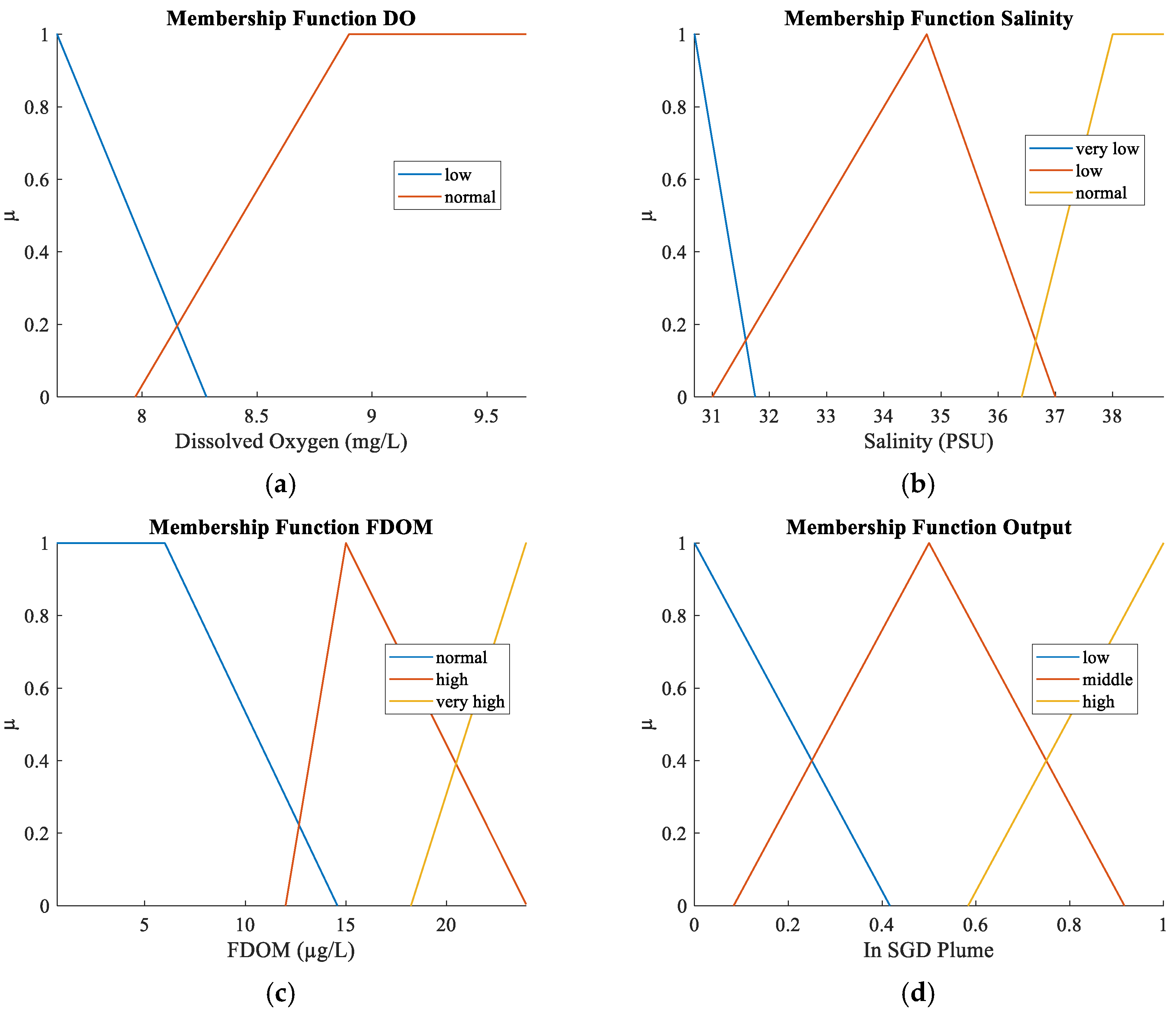In his approach, the rule base, provided by an expert, is given as a set of if–then statements [42]. The use of fuzzy logic requires the definition of several membership-functions for all inputs and outputs, and a set of rules operating on the defined membership functions of the input variables, calculating the output value.

In the past, fuzzy logic has been applied to a vast number of problems in a variety of different fields. These, for instance, include: control-theory [41], crack detection in beams [43], fire detection in engines and batteries [44], pavement section classification [45], characterisation of large changes in wind power [46], path planning and obstacle avoidance of mobile unmanned robots [47,48], and analysing the effect of traffic noise on the human work efficiency [42].

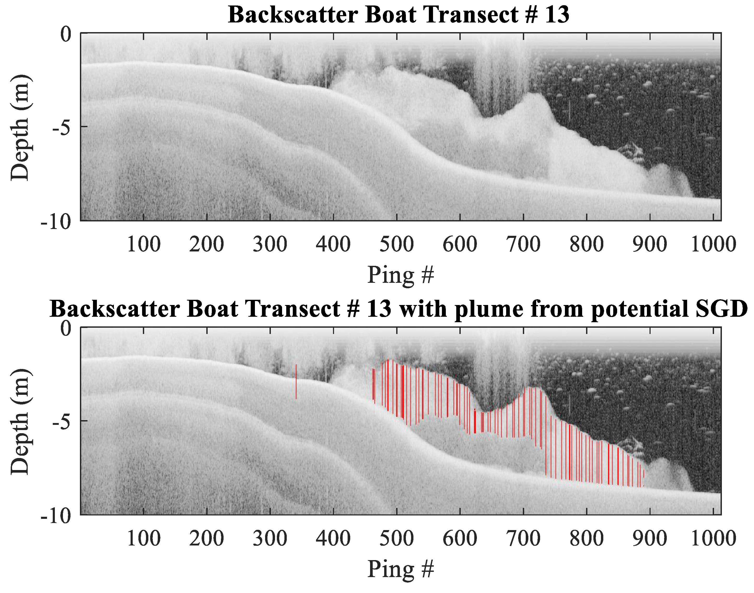
This paper will address the following research questions: (1) can recreational sonars be used for the identification and investigation of the spatial distribution of SGD plumes? (2) To what extent can a low-cost observational ROV, equipped with low-cost sensors be used for the identification and in situ investigation of focused SGD plumes? (3) Can the application of fuzzy logic increase the ability of identifying SGDs using in situ data sampled by ROVs?

2. Materials and Methods

In the first part of this section, information about the study site is given. This includes information about location, bathymetry, groundwater properties, and tides. Afterwards both survey methods used in this study are described.

2.1. Study Site

This study was conducted in Northern Harbour, located in the Woodman Point area near Perth (Western Australia). The area is connected to the Cockburn Sound, a sheltered areal between Garden Island and the Australian Mainland (Figure 2c).

The region of Perth has been in the focus of SGD research for more than 40 years [49]. Due to the geological conditions, especially the large limestone formations and the extensive groundwater resources, the Perth region offers excellent conditions for the formation of underwater springs [21,50]. More information about the hydrogeology settings and the aquifers of the study area can be found in [51] or [21].

In previous studies, several underwater springs in the region of Northern Harbour were detected using a 3.5 kHz seismic profiler [21]. The majority of these springs were found at a depth of approximately 10 m.

Water depth in the Northern Harbour varies between two and ten metres. Starting from the north end of the harbour, water depth remains relatively constant between two and four metres. However, approximately at a distance between 80 and 100 m to the shore water depth increases within a couple of metres to ten metres. Due to a change in the hydraulic conditions, this sharp brim is expected to facilitate the development of focused SGD spots. A bathymetry map of the harbour, based on LIDAR provided by [52], is given in Figure 3.

Smith et al. [21] reported discharge of fresh groundwater into Northern Harbour. The authorities monitor groundwater properties on a regular basis using groundwater wells. Time series data of four different groundwater wells, provided on a daily basis by the Department of Water and Environmental Regulation [53], are used to characterise groundwater properties in this paper. Mean temperature in °C and mean electric conductivity in mS/cm are presented in Figure 4.

As shown in Figure 4, electric conductivity values of groundwater wells ID61470343 and ID61470346 are more stable during the year, while the values of the other two wells are more variable. Compared to Figure 2, wells ID61470343 and ID61470346 are located more landwards than the other two wells. Hence, variability might be caused by seasonal effects resulting in a movement of the freshwater-saltwater interface [1]. However, the temperature of the groundwater seems to be stable during the year. Additional information about the wells is summarised in

Table 1. Summary of position information, drilled depths, and distance from the survey area of the groundwater wells and tide station.

	ID 61470343	ID 61470345	ID 61470346	ID 61470348	Tide Station
Latitude	−32.121876803	−32.120602222	−32.177246642	−32.177533533	−32.065543
Longitude	115.774748305	115.765828397	115.792420959	115.785749627	115.748067
Depth drilled (m)	47.0	30.0	30.0	35.0	n.a.
Distance from survey area (km)	2.27	2.08	5.14	4.84	8.35

.

Previously published research revealed an SGD flowrate dependency on the tidal cycle [6,12,13,21]. In these studies, the SGD flowrate measured or estimated was negatively correlated with the height of the tide. Tide information, covering the time the survey took place, was taken from the tide station located at Fremantle Fishing Boat Harbour. This station is maintained by the Western Australia Department of Transport and the data is publicly available [54]. Position information of the station is included in Table 1. The water height is recorded in five-minute intervals. Figure 5 shows water height at the tide station, as well as begin and end of the sonar and the ROV survey. It can be seen that both the sonar and the ROV survey took place during rising tide.

2.2. Sonar Survey

A skiff, equipped with an echo sounder and a GPS device, was used for the collection of sonar data. The area under investigation was covered by 13 transects. Data collection was focused on the area of the brim. During these transects, georeferenced acoustic backscatter data was recorded using an Humminbird 898 SI echo-sounder [55]. More information about device specifications is summarised in

Table 2. Summary of the specifications of the sonar survey equipment used.

Parameter	Value
Z-resolution	2.5 cm
Update rate	6 Hz
Beam frequency	200 kHz
Beam width	20°
GPS accuracy	2.5 m

. The paths of the different transects are shown in Figure 6. As shown, the whole harbour, except the shallow nearshore areas, were covered by sonar transects.

2.3. In Situ Data Collection (ROV Survey)

When fresh groundwater is discharged into the harbour, electric conductivity and temperature values are expected to be lower in the region of discharge, based on EC and temperature data from the groundwater wells (Figure 4) and the data presented in [21]. In addition, DO is usually depleted in groundwater, due to chemical reactions. Recent studies reported enriched DO values in some pore water samples caused by seawater intrusion. However, the DO values are usually reduced by chemical reaction within the tidal zone [56,57,58]. Furthermore, Suric et al. [59] observed low DO values of SGDs within karst aquifers. Hence, low DO values are expected near SGDs during the in situ surveys. Recent studies found enriched FDOM values in the region of SGDs [60]. Therefore, higher FDOM values are expected to be a proxy for SGDs in this study.

A BlueROV 2 low-cost Remotely Operated Vehicle (ROV) was used as a multi-sensor platform in this research (Figure 7). The ROV carried an integrated in situ sensor system, which was developed in this project. It was equipped with seven environmental low-cost sensors. The sensor system was capable of measuring temperature (T), pressure (P), electric conductivity (EC), dissolved oxygen (DO), oxidation-reduction-potential (ORP), pH, and dissolved organic matter fluorescence (FDOM) concentration. The specifications of the sensors used are summarised in

Table 3. Summary of in situ sensor specifications integrated into the multi-sensor system.

Parameter	Range	Accuracy	Sample Rate	Distributor
Temperature	−5–50 °C	0.1 °C	100 Hz *	BlueRobotics
Pressure	0–30 bar	0.2 bar	50 Hz *	BlueRobotics
Dissolved Oxygen	0.01–100 mg/L	0.05 mg/L	1 Hz	Atlas Scientific
pH	0.007–14.000	0.002	1 Hz	Atlas Scientific
Oxidation-Reduction Potential	−1019.9–1019.9 mV	1 mV	1 Hz	Atlas Scientific
Electric Conductivity	5–200,000 µS/m	2%	1 Hz	Atlas Scientific
Dissolved Organic Matter Fluorescence	0–200 µg/L QSE **	0.04 µg/L QSE **	0.33 Hz	Trios

* Theoretical maximal sample rate of used chip. ** QSE: quinine sulphate equivalent units.

. All sensors were connected to a central microcontroller unit. This microcontroller triggered and collected readings from the different sensors and stored the values, together with a timestamp for later use. Each sensor had its own controller unit, handling the respective sensor readings and the parameter value calculation. The sensor controllers, except for the FDOM sensor controller, were connected to the microcontroller using the I²C-bus. The digital transmission of the sensor values prevented the introduction of noise during the transmission between the sensor controller and the central microcontroller. Due to the analogue transmission of the FDOM value, the signal from this sensor needed to be filtered during post-processing, in order to minimise the effect of measurement noise. The majority of the sensors used in this research were successfully used for environmental studies using unmanned vehicles in recently published research [61,62].

To reference in situ data, sampled by the multi-sensor platform, in a global coordinate system, the platform is equipped with an acoustic transmitter. This transmitter is part of a commercial Short Baseline system (SBL). The transmitter emits acoustic signals, which are than received by four acoustic receivers, mounted on the surface vessel. The relative position of the ROV and the surface vehicle then can be calculated by trilateration [37,63]. Figure 8a shows a sketch of this setup, containing the ROV equipped with an acoustic transmitter (1) and four acoustic receivers (2) attached to the surface vessel, equipped with a GNSS receiver (3). All global positions are represented using the Map Grid of Australia zone 50 reference system (MGA50) [64], allowing simple transformation and calculations between two points. The global position of the ROV was calculated based on the known global position of the surface vessel and the acoustically measured relative position of the ROV as follows:

P = O + R·X,

(1)

with:

$\mathrm{P}$	Global position of the ROV as: $\mathrm{P}=\left[\begin{array}{c}\mathrm{Easting}\\ \mathrm{Northing}\end{array}\right]$,
$\mathrm{O}$	Global position of the boat (origin) as: $\mathrm{O}=\left[\begin{array}{c}\mathrm{Easting}\\ \mathrm{Northing}\end{array}\right]$,
$\mathrm{R}$	Rotation matrix as: $\mathrm{R}=\left[\begin{array}{cc}cos\left(360°-\mathsf{\theta }\right)& sin\left(360°-\mathsf{\theta }\right)\\ -sin\left(360°-\mathsf{\theta }\right)& cos\left(360°-\mathsf{\theta }\right)\end{array}\right]$,
$\mathrm{X}$	Relative position of the ROV as $\mathrm{X}=\left[\begin{array}{c}\mathrm{x}\\ \mathrm{y}\end{array}\right]$,
$\mathsf{\theta }$	Heading of the boat in degree.

To survey the whole harbour area during data collection, the boat was tethered to a jetty at three different positions. Hence, due to the fixed boat positions, the heading of the boat did not change during the ROV surveys. The boat positions are marked in Figure 8b. In addition, the areas in which the ROV surveys took place are marked by polygons.

During the surveys, position information was recorded with a frequency of 20 Hz. During post-processing, data were resampled and repeated tuples were removed from the data set. After resampling, 23,796 position tuples remained in the data set. Afterwards, outliers were removed. A point was classified as outlier if the value was three standard deviations away from the moving median. The moving window size was set to 59 samples. This reduced the number of tuples to 22,897, i.e., 3.78% of the position tuples were detected as outliers and removed from the data set. Furthermore, the data set was split in three parts, according to the three different positions of the skiff given in Figure 8b. At the second location, the surface vessel was located close to a jetty and between two concrete blocks. Hence, the acoustic conditions were corrupted and the position estimations, recorded at this location, are affected by additional large errors. Therefore, position data recorded from the second location was not used in this study. Thus, 6859 tuples, or 28.8%, were dropped from the data set.

The sensor system recorded 9666 data points during the surveys. The sensor system was not turned off between the surveys, for example during the transitions of the surface vessel to another location. Hence, the data set also includes tuples where the ROV was not submerged. After removing this data, 5688 tuples, or 58.85%, remained in the environmental data set. The remaining data was split into three subsets according to the three different positions of the surface vessel.

Both position and environmental data were then synchronised using autocorrelation between the recorded depth and pressure values. Afterwards, the position data were interpolated to obtain equal-sized data sets.

2.4. Fuzzy Logic Applied to SGD Detection

As mentioned above, the sensor system developed carried seven sensors for different kinds of environmental parameters. In this research DO, salinity and FDOM readings are merged using a fuzzy logic approach. The membership functions for the three input values DO, salinity, and FDOM were defined based on the statistical data summarised in

Table 4. Fuzzy rule base applied for SGD identification based on human expert knowledge.

Rule	Salinity	DO	FDOM	Output
#1	low	low	-	high
#2	-	low	high	high
#3	low	-	very high	high
#4	very low	-	high	high
#5	low	-	high	middle
#6	very low	low	high	high
#7	normal	normal	normal	low
#8	normal	normal	high	middle
#9	normal	low	normal	middle
#10	low	normal	normal	middle

and the expected behaviour of the parameters in proximity of discharged groundwater. For DO, two membership functions, named low and normal, were defined. The low membership function decreases from one, at the recorded minimum of 7.63 mg/L, to zero at 8.25 mg/L. This value corresponds to the minimum plus two times the standard deviation. The normal membership functions starts rising at a DO value of 7.97 mg/L (mean minus three times standard deviation). It reaches the maximum at the DO mean value, i.e., 8.9 mg/L. For salinity, three membership functions, named very low, low, and normal, were defined. In addition, three membership functions named normal, high, and very high were defined for FDOM. Similar to the DO membership functions, normal and very low salinity and normal and very high FDOM membership functions are based on statistical data. However, to cover the whole input space, a third membership function was introduced for salinity and FDOM, called low and high, respectively. All membership functions designed are shown in Figure 9.

Rules in fuzzy logic are based on the knowledge of experts in the field to which fuzzy logic is applied. In this research, rules were formulated based on the previously discussed expected behaviour of the three parameters in the proximity of discharged fresh groundwater. Using the defined membership functions (Figure 9), ten rules were formulated in order to identify measurements, which were potentially taken in proximity of an SGD plume. The rules are summarised in Table 4.

Membership functions and rules are implemented as Mamdani fuzzy inference system [65] using the “Fuzzy Logic Designer” from Matlab’s Fuzzy Logic Toolbox [66]. This toolbox has been used to develop fuzzy logic systems in recent research [42,47]. Obtaining estimations from the fuzzy logic inference system requires defuzzification [67]. In this research, a centroid defuzzification scheme was applied.

3. Results

Data captured during the surveys is analysed in this section. The whole post processing of the data is undertaken using the Matlab environment. In the first subpart, results from the sonar surveys are presented in two different ways: (1) a bathymetry map based on recorded depth information is generated and compared with the bathymetry map shown in Figure 3. In addition, echograms of the different transects are presented and potential SGD plumes are identified. In the second subsection, in situ environmental parameter data, recorded during the ROV surveys, are presented within time series, depth profiles and spatial distribution plots. Potential areas of SGD influence are identified within the spatial distribution plots.

3.1. Sonar Survey

During the sonar surveys, depth and position information was stored for later use. This data was used to generate a bathymetry map, shown in Figure 10. The water depths recorded varied from 0.4 m to 9.1 m within the investigated harbour area. It can be observed from the figure that there is a steep slope in water depths in the area under investigation. The recorded bathymetry data does fit the bathymetry data provided by LIDAR measurements shown in Figure 3.

In addition, echo sounder data was used to identify possible SGD plumes. It has been shown in recent studies that the composition of discharged water from an SGD can differ from the composition of the receiving water body [6,13]. Due to these differences, the acoustic properties of the discharged water differ from the properties of the receiving water body, enabling an identification of the discharged water using echo sounders. A human expert, who marked potential SGD plumes based on their knowledge base, reviewed all echograms recorded during the study. Acoustic anomalies were marked as potential SGD plumes due to homogenous high backscatter, its connection to the seafloor, and stable temporal behaviour, i.e., if the anomalies appeared in different echograms covering the same area. Figure 11 shows the echogram recorded during transect number 13. The area of a potential SGD plume is marked in red. It can be observed that the potential SGD spot was located near the brim. The human expert identified a total number of 23 potential plumes within all recorded sonar transects. However, as shown in Figure 6, the transects overlap at some points, covering identical parts of the area under investigation. The echograms of the other sonar transects, including the identified potential SGD plumes, can be found in Supplementary Material Figure S1.

3.2. In Situ Data Collection (ROV Survey)

This chapter focuses on the in situ recorded environmental data. Data were processed in three different ways. First, time series plots for all different parameters are presented. Time series can be used to detect drifts in data, provoked by various effects, for example tides. Secondly, depth profiles are presented. Some parameters, like temperature, vary with different depth, according to physical effects. Therefore, depth profiles might help to identify data that do not follow these depth dependencies, and hence may represent data sampled in proximity to discharged freshwater. Lastly, spatial distribution plots are presented. These plots were used to identify potential areas of abnormal parameter values, which might indicate discharged fresh groundwater.

3.2.1. Time Series

During the ROV survey, in situ sensors, mounted underneath the ROV, measured different environmental parameters. Time series of the different parameters are provided in Figure 12. Temperature was volatile, with values between 21.93 °C and 23.62 °C. EC values were stable around 54 mS/cm, only showing some readings with lower values. Temperature and electric conductivity values were used to calculate the salinity according to the formulations given by the UNESCO 1983 standard [68]. Thus, salinity values reflected the variability of the temperature time series. DO values were ranging from 8.5 mg/L to 9.5 mg/L with some remarkable low values. The minimum DO value measured was 7.63 mg/L. The pH readings were stable during the whole survey. Except for the beginning of the first survey, pH values were varying around the mean value of 8.2. The low values seemed to be outliers, affected by air bubbles or other effects. The ORP value was constantly increasing over time. However, the time series indicated some significant dips in the ORP value correlated with dips in other environmental parameters like DO, salinity, or FDOM. As expected, FDOM values were affected by measurement noise. However, some significant peaks were identified, which may indicate freshwater from a SGD. Pressure readings varied during the survey, reflecting the different dive depths of the ROV. Pressure values were used to calculate dive depths according to the algorithms given in [68]. Mean, standard deviation, minimum, and maximum values for the different parameters are summarised in

Table 5. In situ measurements statistical information summary, based on all data points recorded during ROV surveys. Pressure is not included in this table.

Parameter	Mean	Standard Deviation	Minimum	Maximum
Temperature	22.4 °C	0.43 °C	21.93 °C	23.62 °C
Dissolved Oxygen	8.9 mg/L	0.31 mg/L	7.63 mg/L	9.67 mg/L
pH	8.2	0.03	7.38	8.25
Oxidation-Reduction-Potential	179.6 mV	29.4 mV	123.8 mV	232.5 mV
Electric Conductivity	54.1 mS/cm	0.34 mS/cm	44.4 mS/cm	55.1 mS/cm
Salinity	38.0 PSU	0.53 PSU	30.69 PSU	38.89 PSU
Dissolved Organic Matter Fluorescence	6.0 µg/L QSE *	2.86 µg/L QSE *	0.64 µg/L QSE *	24.0 µg/L QSE *

* QSE: quinine sulphate equivalent units.

.

3.2.2. Depth Profiles

Due to environmental influences, for example solar radiation or density effects, depth-dependent changes for selected parameters, e.g., temperature or EC, can be expected [5]. Therefore, recorded and post-processed environmental data were used for depth profiling. Figure 13 shows depth profiles for T, EC, DO, and FDOM. Depth profiles for the remaining parameters can be found in the supplementary material Figure S2. Depth was calculated from pressure readings using the pressure sensor attached to the multi-sensor system developed. Therefore, even environmental data without a valid position estimation could be used for the depth profiles.

It can be observed from the depth profiles that temperature decreases with increasing depth. This effect is driven by solar radiation and the density dependency of seawater on temperature [68]. The EC values were stable with increasing water depth. However, the EC values at the surface were slightly lower. In addition, few samples with low EC values were measured in depth of approximately 10 m. DO readings had a wider spread than temperature or EC. Additionally, DO seemed to be affected by the water depth. DO values increased from the surface with depth. However, after reaching a depth of approximately 5 m, values decreased with further increased depth. In addition, some samples with lower DO values were measured at depths deeper than 4 m. DO readings used in this study are given in mg/L. However, one needs to take into account that solubility of DO in water depends on temperature, salinity and pressure [69]. The FDOM values seemed to be unaffected by the depth, with high variations of the readings at all depths.

3.2.3. Spatial Distribution

Both time series (Figure 12) and depth profiles (Figure 13) show evidence of an influence of SGD inflow on the environmental parameters. This, for instance, includes the low DO values at depths greater than 5 m, the high FDOM values measured at various depths, and the low salinity values measured at greater depths. However, neither time series nor depth profiles were capable of answering questions about the spatial distribution of the measured values, or, therefore, to indicate a relationship between environmental data and sonar data. Hence, in addition, the spatial distribution of the recorded parameters was investigated. Therefore, all georeferenced in situ data points were split into various transects with a transect width of 5 m. Afterwards all data points located within one transect were interpolated and plotted in the northing-depth plane. Figure 14 shows the location of the different transects as well as the spatial distributions of salinity, DO and FDOM for transect number six. In the spatial distribution plots, black areas indicating the seafloor based on the sonar survey data. The contour plots of the remaining parameters and transects can be found in Supplementary Material Figure S3. From the spatial distribution plots, nine areas with potential SGD plumes were identified. The location of these areas is indicated by red polygons in Figure 14a. It can be seen from the figure that these areas were crossed by different sonar transects. In total, 19 intersections between the sonar transects and the identified areas were counted. The ping numbers, which were recorded within these areas, are summarised in

Table 6. Summary of potential SGD areas identified from spatial distribution plots, and the number of sonar transects crossing these areas with corresponding ping numbers.

Transect Spatial Distribution	Parameter	Northing (×106 m)	Transect Sonar Survey	Ping Numbers Echogram	Plume in Echogram
T2	FDOM	6.44339–6.44341	R16	500–560	Yes
			R17	500–543	Yes
			R23	1134–1176	Yes
			R23	1898–1960	Yes
			R24	1380–1440	Yes
T3	FDOM	6.44339–6.44340	R23	1180–1233	Yes
T4	DO, FDOM	6.44341–6.44343	R16	1–70	Yes
T5	DO, FDOM *	6.443405–6.44325	R16	71–120	Yes
			R16	185–217	No
T6.1	Salinity, DO, FDOM	6.44337–6.44338	R23	1680–1744	No **
T6.2	DO, FDOM *	6.44341–6.44344	R24	3884–3970	No
T7	FDOM	6.44337–6.443385	R23	1610–1680	Yes
			R25	437–467	No ***
			R26	690–708	No
T8	FDOM	6.44338–6.44340	R23	1455–1520	Yes
			R25	468–505	No ***
			R26	675–689	No
T9	FDOM	6.44338–6.44395	R25	505–560	No ***
			R26	655–674	No

* Spatial distribution indicates only small patches with higher values in this area. ** Close to two plumes, plumes end at ping number 1613 and 1754, respectively. *** No plumes were detected in sonar transect R25.

. Furthermore, the table contains information as to whether an echogram shows a plume for this ping number or not.

3.3. Fuzzy Logic Applied to SGD Detection

The fuzzy logic system was used to classify the recorded in situ environmental data. The defuzzied output for all samples is shown in Figure 15a. The fuzzy logic inference system identified 293 data points, i.e., 5.83%, as potentially being located within an SGD plume. The spatial distribution of the identified peaks from ROV surveys one and three are shown in Figure 15b. In addition, the figure shows the position of the sources of the potential SGD plumes, identified from the echograms by the human expert. The minimum distance between the samples identified by fuzzy logic and the plumes identified by sonar are calculated. The in situ data were separated into four subsets, according to the ROV surveys and the output of the fuzzy system (Figure 15c). The mean values and standard deviations for the four different groups are summarised in Figure 15d. One can observe that the mean distance for the first ROV survey is approximately two times the mean distances calculated for the third ROV survey.

4. Discussion

Results from both methods indicate the occurrence of SGDs in the area under investigation. In the first two parts of this chapter, results from sonar and in situ surveys are discussed separately. Afterwards, a fuzzy logic approach is used for identification of SGD plumes. The spatial relation between fuzzy logic output and sonar surveys is discussed.

4.1. Sonar Survey

As shown in Figure 11 and the Supplementary Material Figure S1, the recreational echo sounder used in this study was suitable for detecting various plumes with different sizes and appearances. The majority of the plumes detected appear close to the brim. The appearance and position of these plumes matches the appearance and positions of plumes reported by other researchers, detected during recent studies in the same area [21]. As shown in Figure 6, some parts of the area under investigation were covered by different transects. For instance, one area is covered by the transects R13, R14, R23, and R24. Comparing the echograms of these four transects, it can be observed that the plume, shown in Figure 11, can also be found in the other three transects, given in Supplementary Material Figure S1. One needs to consider that the echograms were generated on basis of the pings sent by the sonar, and do not take into account spatial correspondences with other transects for averaging. Therefore, due to different headings and speeds of the boat during the surveys, the appearance of the plume in the echograms vary. Furthermore, due to different directions the plume was crossed, the echogram of transect R14 needs to be mirrored in order to match the appearance of the other echograms. From the echograms it can be noted that the formed plume does not move straight upwards. It rather flows towards the shallower part of the harbour. Data reported in [21] show that the major part of the discharged groundwater was recirculating seawater. Hence, the density difference between discharged groundwater and the ambient seawater is small. This small difference results in a small upwelling momentum of the discharged seawater [27]. In addition, depth profiles in Figure 13 show a higher surface temperature resulting in a lower density layer at the surface. This lower-density layer might prevent the plume upstreaming to the surface. As mentioned before, the survey took place during rising tide, so seawater pushes into the harbour, potentially resulting in currents flowing from south to north (Figure 2). Current profiles were not recorded during this study. However, the ROV pilot encountered strong currents during ROV operation in the intended direction.

4.2. In Situ Data Collection (ROV Survey)

The time series indicates a high dynamic change of the temperature over time. However, depth profiles show a clear relation between temperature and depth. From spatial analyses, no effect of discharged water on the temperature can be observed. This result does not comply with the results reported by other researchers [7,19]. As shown in Figure 4 and reported in [21], groundwater temperature in the region of Perth is almost stable during the year. Groundwater temperature of the four different groundwater wells (Table 1) varies between 20.5 °C and 21.1 °C over the entire year, while the average temperature of the surrounding water column was 22.4 °C, with lower values at greater depths. Mean temperature for all readings taken from a depth greater than 8 m was 21.98 °C. Maybe, due to mixing processes between discharged and surrounding water, temperature differences become too small to measure instantly after discharging took place.

EC values are stable over time, varying around the average value of 54.1 mS/cm. The depth profile only indicates lower values in very shallow depth without any further depth relations. However, both, time series and depth profile, indicate a certain number of readings with significantly lower EC values, pointing towards discharge from a SGD. Furthermore, the profile shows a higher variation of the EC near the surface. This may indicate a layer of slightly fresher water at the surface, due to buoyancy effects.

Salinity is not measured independently; values are rather calculated based on measured temperature and EC values. Hence, the salinity time series combines the characteristic of both temperature and EC time series, i.e., significant peaks from both can be identified within the salinity time series. The depth profile points out an increase in salinity with depth, based on the temperature–depth relation described above.

DO values vary over time. Comparison with the pressure time series indicates a depth dependency of DO values. DO depth profile shows increasing DO values with increasing depth until a depth of 5 m; afterwards, DO values decrease with further increasing depth. Noticeable low values at a depth of approximately 9 m may indicate groundwater inflow. Time series show an increase of DO values after timestamp 6000 s. This increase could be explained by wind-introduced waves increasing the solubility of oxygen in the upper water column. The Perth region is known for very strong afternoon sea breezes during summer months [70].

The time series of pH shows stable values over time, varying around the mean value of 8.2. No indications for an influence of discharged water on the pH value can be observed. Hence, pH will be analysed no further in this paper.

The time series show a constant increase of ORP over time. This behaviour does not indicate the true ORP values, but error-affected measurements, caused by improper electrical connections [71]. However, some noticeable dips in ORP correspond with dips in the other time series, for example DO or FDOM. Nevertheless, due to the uncertain behaviour, ORP data will not be used for further analyses.

The FDOM time series shows a high variation, potentially introduced by analogue communication between the central microcontroller and the sensor. Furthermore, time series indicates some noticeable high sensor readings corresponding with indicated low values in DO and salinity may denote groundwater inflow. However, depth profile does not imply a depth relation of FDOM values.

The spatial distribution of the environmental parameters shown in Figure 14 indicates an area with a depth between 6 m and 8 m, where the salinity and DO values are decreased and the FDOM values are increased. As mentioned previously, this behaviour of the three parameters can be expected when an area is influenced by discharged freshwater from a SGD. In addition, DO and FDOM anomalies can be found in seven other spatial distribution transects, given in Figure S3. All of these areas were crossed by different sonar transects. Further information is summarised in Table 6. It can be observed that 10 echogram intersections out of 19 show evidence for SGD plumes. Some of the intersections only cover a very small part of the intended area. In addition, due to different sampling times for both data sets, the appearance of the plumes might have changed between the surveys.

4.3. Fuzzy Logic Applied to SGD Detection

The fuzzy system developed identified 5.83% of the in situ samples as being “in SGD plume”. Some of the points, identified using the fuzzy system, correspond well with the potential SGD positions identified by the human expert, while the majority of the identified positions are aggregated in a region in the upper left part of the figure. Referring to Figure 6, this area was not covered by sonar transects. Therefore, no sonar information is available for this part of the area.

The in situ data were separated into four subsets, according to the ROV surveys and the output of the fuzzy system. It can be observed from Figure 15d that the mean values for the first survey are higher than the mean values of the third survey. However, in both cases the mean values for the points classified by the fuzzy system, as “in SGD plume” are smaller than the mean values for the points classified as not in plume. In addition, for both surveys, the standard deviation of the “in SGD plume” points is lower than the standard deviation of the other output class.

In this research, sensor fusion took place during post-processing of the sensor data. However, to facilitate online identification of SGD sites, the fuzzy logic system developed will be implemented on the on-board microcontroller of the multi-sensor system for further observations.

In addition, the sonar survey and the ROV survey were conducted subsequently. This may lead to misinterpretations, when both data sets are analysed together. In the future, both surveys should take place at the same time. Furthermore, a sonar attached to the ROV could allow for the simultaneous collection of echograms and environmental data. In recently published research, a low-cost scanning sonar was used to track microbubble plumes [72]. Thus, this technique can potentially be used for SGD plumes as well.

In this study, real SGD sites were investigated using novel methods and equipment. However, no data from other well-established methods, like CTD or in situ radon measurements, are available for verification of these novel methods. Thus, further investigations, combining this novel and other well-established methods, should be considered to verify the abilities and constrains of both sonar and ROV systems in more detail. In addition, using an artificial SGD could be a potential way to capture ground truth data.

5. Conclusions

The focus of this research was the investigation of SGD sites using low-cost equipment. Various potential SGD plumes were detected using a skiff equipped with a recreational echo sounder. Patterns were classified as SGD plumes according to the assumptions that SGD plumes are connected to the sea floor and that the appearance of the patterns is stable at least over a short period of time. It was demonstrated that this inexpensive equipment can be used to detect plumes in coastal areas. However, it remains an open task to verify with an independent method that the plumes are formed by SGDs.

In addition, results from in situ ROV observations were discussed. Spatial distribution of salinity, DO and FDOM indicate SGD sites corresponding to plumes identified during the sonar survey. To enhance SGD detection, the recorded sensor data were post-processed; for instance, data were filtered and resampled. In this study, not all in situ parameters, for instance pH or ORP, could be used to identify SGDs.

Furthermore, fuzzy logic was applied to the fusion of salinity, DO, and FDOM readings in order to enhance SGD detection capability of the presented multi-sensor system. Results of the fuzzy logic approach correspond well with the position of the plumes identified during the sonar survey.

Low-cost ROVs, equipped with environmental sensors, can be an important tool for the investigation of the spatio-temporal behaviour of SGD sites. This method allows continuous mapping of environmental parameters with a high spatial and temporal resolution. However, to obtain deeper insights into the influence of SGDs on the nearshore areas, this method should be combined with other well-established methods for SGD investigation, such as pore water sampling, remote sensing, or groundwater monitoring.

References

1. Burnett, W.; Aggarwal, P.; Aureli, A.; Bokuniewicz, H.; Cable, J.; Charette, M.; Kontar, E.; Krupa, S.; Kulkarni, K.; Loveless, A.; et al. Quantifying submarine groundwater discharge in the coastal zone via multiple methods. Sci. Total Environ. 2006, 367, 498–543. [Google Scholar] [CrossRef]
2. Moore, W.S. The Effect of Submarine Groundwater Discharge on the Ocean. Annu. Rev. Mar. Sci. 2010, 2, 59–88. [Google Scholar] [CrossRef] [PubMed] [Green Version]
3. Lane-Smith, D.; Burnett, W.C.; Kim, G. A continuous monitor for assessment of 222Rn in the coastal ocean. J. Radioanal. Nucl. Chem. 2001, 249, 167–172. [Google Scholar] [CrossRef]
4. Tholen, C.; Nolle, L.; Zielinski, O. On the effect of neighborhood schemes and cell shape on the behaviour of cellular automata applied to the simulation of submarine groundwater discharge. In Proceedings of the 31st Conference on Modelling and Simulation, ECMS 2017, Budapest, Hungary, 23–26 May 2017; Paprika, Z.Z., Horák, P., Váradi, K., Zwierczyk, P.T., Vidovics-Dancs, Á., Rádics, J.P., Eds.; ECMS: UK, 2017; pp. 255–261, ISBN 9780993244049. [Google Scholar]
5. Surić, M.; Lončarić, R.; Buzjak, N.; Schultz, S.T.; Šangulin, J.; Maldini, K.; Tomas, D. Influence of submarine groundwater discharge on seawater properties in Rovanjska-Modrič karst region (Croatia). Environ. Earth Sci. 2015, 74, 5625–5638. [Google Scholar] [CrossRef]
6. Peterson, R.N.; Burnett, W.C.; Glenn, C.R.; Johnson, A.G. Quantification of point-source groundwater discharges to the ocean from the shoreline of the Big Island, Hawaii. Limnol. Oceanogr. 2009, 54, 890–904. [Google Scholar] [CrossRef]
7. Lee, E.; Yoon, H.; Hyun, S.P.; Burnett, W.C.; Koh, D.; Ha, K.; Kim, D.; Kim, Y.; Kang, K. Unmanned aerial vehicles (UAVs)-based thermal infrared (TIR) mapping, a novel approach to assess groundwater discharge into the coastal zone. Limnol. Oceanogr. Methods 2016, 14, 725–735. [Google Scholar] [CrossRef]
8. Mallast, U.; Siebert, C. Combining continuous spatial and temporal scales for SGD investigations using UAV-based thermal infrared measurements. Hydrol. Earth Syst. Sci. 2019, 23, 1375–1392. [Google Scholar] [CrossRef] [Green Version]
9. Spalt, N.; Murgulet, D.; Abdulla, H. Spatial variation and availability of nutrients at an oyster reef in relation to submarine groundwater discharge. Sci. Total Environ. 2020, 710, 136283. [Google Scholar] [CrossRef]
10. Luijendijk, E.; Gleeson, T.; Moosdorf, N. Fresh groundwater discharge insignificant for the world’s oceans but important for coastal ecosystems. Nat. Commun. 2020, 11, 1260. [Google Scholar] [CrossRef] [PubMed] [Green Version]
11. Slomp, C.P.; Van Cappellen, P. Nutrient inputs to the coastal ocean through submarine groundwater discharge: Controls and potential impact. J. Hydrol. 2004, 295, 64–86. [Google Scholar] [CrossRef] [Green Version]
12. Taniguchi, M. Tidal effects on submarine groundwater discharge into the ocean. Geophys. Res. Lett. 2002, 29, 2.1–2.3. [Google Scholar] [CrossRef]
13. Sholkovitz, E.; Herbold, C.; Charette, M. An automated dye-dilution based seepage meter for the time-series measurement of submarine groundwater discharge. Limnol. Oceanogr. Methods 2003, 1, 16–28. [Google Scholar] [CrossRef] [Green Version]
14. Israelsen, O.W.; Reeve, R.C. Canal Lining Experiments in the Delta Area Utah, UT, USA. 1944. Available online: https://digitalcommons.usu.edu/uaes_bulletins/348/ (accessed on 1 April 2020).
15. Lee, D.R. A device for measuring seepage flux in lakes and estuaries. Limnol. Oceanogr. 1977, 22, 140–147. [Google Scholar] [CrossRef]
16. Taniguchi, M.; Fukuo, Y. Continuous Measurements of Ground-Water Seepage Using an Automatic Seepage Meter. Ground Water 1993, 31, 675–679. [Google Scholar] [CrossRef]
17. Paulsen, R.J.; Smith, C.F.; O’Rourke, D.; Wong, T.-F. Development and Evaluation of an Ultrasonic Ground Water Seepage Meter. Ground Water 2001, 39, 904–911. [Google Scholar] [CrossRef] [PubMed]
18. Seibert, S.L.; Degenhardt, J.; Ahrens, J.; Reckhardt, A.; Schwalfenberg, K.; Waska, H. Investigating the Land-Sea Transition Zone. In YOUMARES 9—The Oceans: Our Research, Our Future, Proceedings of the 2018 Conference for YOUng MArine RESearcher, Oldenburg, Germany, 11–14 September 2018, 1st ed.; Jungblut, S., Liebich, V., Bode-Dalby, M., Eds.; Springer International Publishing: Cham, Switzerland, 2020; pp. 225–242. ISBN 978-3-030-20389-4. [Google Scholar]
19. Mallast, U.; Schwonke, F.; Gloaguen, R.; Geyer, S.; Sauter, M.; Siebert, C. Airborne Thermal Data Identifies Groundwater Discharge at the North-Western Coast of the Dead Sea. Remote Sens. 2013, 5, 6361–6381. [Google Scholar] [CrossRef] [Green Version]
20. Taniguchi, M.; Dulai, H.; Burnett, K.M.; Santos, I.; Sugimoto, R.; Stieglitz, T.; Kim, G.; Moosdorf, N.; Burnett, W.C. Submarine Groundwater Discharge: Updates on Its Measurement Techniques, Geophysical Drivers, Magnitudes, and Effects. Front. Environ. Sci. 2019, 7, 335. [Google Scholar] [CrossRef]
21. Smith, A.J.; Herne, D.E.; Hick, W.P.; Turner, J.V. Quantifying Submarine Groundwater Discharge and Nutrient Discharge into Cockburn Sound Western Australia: A Technical Report to the Coast and Clean Seas Project WA9911: Quantifying Submarine Groundwater Discharge and Demonstrating Innovative Clean-Up to Protect Cockburn Sound from Nutrient Discharge; CSIRO: Wembley, WA, Australia, 2003; ISBN 0643061134. [Google Scholar]
22. Stieglitz, T.; Ridd, P. Submarine Groundwater Discharge from Paleochannels?: “Wonky Holes” on the Inner Shelf of the Great Barrier Reef. In Hydro 2000: Interactive Hydrology, Proceedings of the 3rd International Hydrology and Water Resources Symposium of the Institution of Engineers, Sheraton Perth Hotel, Perth, WA, Australia, 20–23 November 2000; Institution of Engineers, Australia: Barton, ACT, Australia, 2000; pp. 189–194. ISBN 0957824114. [Google Scholar]
23. Taniguchi, M. Change in Groundwater Seepage Rate into Lake Biwa, Japan. Jpn. J. Limnol. 1995, 56, 261–267. [Google Scholar] [CrossRef] [Green Version]
24. Stieglitz, T.; Rapaglia, J.; Bokuniewicz, H. Estimation of submarine groundwater discharge from bulk ground electrical conductivity measurements. J. Geophys. Res. Space Phys. 2008, 113, 17. [Google Scholar] [CrossRef]
25. Street, J.H.; Knee, K.L.; Grossman, E.E.; Paytan, A. Submarine groundwater discharge and nutrient addition to the coastal zone and coral reefs of leeward Hawai’i. Mar. Chem. 2008, 109, 355–376. [Google Scholar] [CrossRef]
26. Cable, J.E.; Bugna, G.C.; Burnett, W.C.; Chanton, J.P. Application of 222 Rn and CH4 for assessment of groundwater discharge to the coastal ocean. Limnol. Oceanogr. 1996, 41, 1347–1353. [Google Scholar] [CrossRef]
27. Munwes, Y.Y.; Geyer, S.; Katoshevski, D.; Ionescu, D.; Licha, T.; Lott, C.; Laronne, J.B.; Siebert, C. Discharge estimation of submarine springs in the Dead Sea based on velocity or density measurements in proximity to the water surface. Hydrol. Process. 2020, 34, 455–472. [Google Scholar] [CrossRef]
28. Christ, R.D.; Wernli, R.L. (Eds.) The ROV Manual: A User Guide to Observation-Class Remotely Operated Vehicles, 1st ed.; Elsevier Butterworth-Heinemann: Amsterdam, The Netherlands; Boston, MA, USA; London, UK, 2011; ISBN 9780750681483. [Google Scholar]
29. Capocci, R.; Dooly, G.; Omerdić, E.; Coleman, J.; Newe, T.; Toal, D. Inspection-Class Remotely Operated Vehicles—A Review. J. Mar. Sci. Eng. 2017, 5, 13. [Google Scholar] [CrossRef]
30. Brodeur, R. In situ observations of the association between juvenile fishes and scyphomedusae in the Bering Sea. Mar. Ecol. Prog. Ser. 1998, 163, 11–20. [Google Scholar] [CrossRef] [Green Version]
31. Klump, J.V.; Paddock, R.; Lovalvo, D. A Multiple-Loop, ROV Controlled, In-Situ Water Sampler. J. Great Lakes Res. 1992, 18, 309–315. [Google Scholar] [CrossRef]
32. Buscher, E.; Mathews, D.L.; Bryce, C.; Bryce, K.; Joseph, D.; Ban, N.C. Applying a Low Cost, Mini Remotely Operated Vehicle (ROV) to Assess an Ecological Baseline of an Indigenous Seascape in Canada. Front. Mar. Sci. 2020, 7, 554. [Google Scholar] [CrossRef]
33. Garner, S.B.; Olsen, A.M.; Caillouet, R.; Campbell, M.D.; Iii, W.F.P. Estimating reef fish size distributions with a mini remotely operated vehicle-integrated stereo camera system. PLoS ONE 2021, 16, e0247985. [Google Scholar] [CrossRef] [PubMed]
34. Rofallski, R.; Tholen, C.; Helmholz, P.; Parnum, I.; Luhmann, T. Measuring Artificial Reefs using a Multi-Camera System for Unmanned Underwater Vehicles. Int. Arch. Photogramm. Remote Sens. Spatial Inf. Sci. 2020, XLIII-B2-2020, 999–1008. [Google Scholar] [CrossRef]
35. De Lima, R.L.P.; Boogaard, F.C.; de Graaf-van Dinther, R.E. Innovative Water Quality and Ecology Monitoring Using Underwater Unmanned Vehicles: Field Applications, Challenges and Feedback from Water Managers. Water 2020, 12, 1196. [Google Scholar] [CrossRef] [Green Version]
36. Wu, Y.; Ta, X.; Xiao, R.; Wei, Y.; An, D.; Li, D. Survey of underwater robot positioning navigation. Appl. Ocean Res. 2019, 90, 101845. [Google Scholar] [CrossRef]
37. Paull, L.; Saeedi, S.; Seto, M.; Li, H. AUV Navigation and Localization: A Review. IEEE J. Ocean. Eng. 2014, 39, 131–149. [Google Scholar] [CrossRef]
38. Khaleghi, B.; Khamis, A.; Karray, F.O.; Razavi, S.N. Multisensor data fusion: A review of the state-of-the-art. Inf. Fusion 2013, 14, 28–44. [Google Scholar] [CrossRef]
39. Kim, T.; Park, T.-H. Extended Kalman Filter (EKF) Design for Vehicle Position Tracking Using Reliability Function of Radar and Lidar. Sensors 2020, 20, 4126. [Google Scholar] [CrossRef] [PubMed]
40. Zadeh, L.A. FUZZY SETS. In Fuzzy Sets, Fuzzy Logic, and Fuzzy Systems: Selected Papers by Lotfi A. Zadeh; Zadeh, L.A., Yuan, B., Klir, G.J., Eds.; World Scientific Pub. Co.: Singapore; River Edge, NJ, USA, 1996; pp. 394–432. ISBN 9789810224219. [Google Scholar]
41. Mamdani, E.H. Application of Fuzzy Logic to Approximate Reasoning Using Linguistic Synthesis. IEEE Trans. Comput. 1977, C-26, 1182–1191. [Google Scholar] [CrossRef]
42. Pal, D.; Bhattacharya, D. Effect of Road Traffic Noise Pollution on Human Work Efficiency in Government Offices, Private Organizations, and Commercial Business Centres in Agartala City Using Fuzzy Expert System: A Case Study. Adv. Fuzzy Syst. 2012, 2012, 828593. [Google Scholar] [CrossRef] [Green Version]
43. Dash, A.K. Analysis of Adaptive Fuzzy Technique for Multiple Crack Diagnosis of Faulty Beam Using Vibration Signatures. Adv. Fuzzy Syst. 2013, 2013, 164853. [Google Scholar] [CrossRef] [Green Version]
44. Dattathreya, M.S.; Singh, H.; Meitzler, T. Detection and Elimination of a Potential Fire in Engine and Battery Compartments of Hybrid Electric Vehicles. Adv. Fuzzy Syst. 2012, 2012, 687652. [Google Scholar] [CrossRef] [Green Version]
45. Mahmood, M.; Rahman, M.; Nolle, L.; Mathavan, S. A fuzzy logic approach for pavement section classification. Int. J. Pavement Res. Technol. 2013, 6, 620–626. [Google Scholar] [CrossRef]
46. Martinez-Arellano, G.; Nolle, L.; Cant, R.; Lotfi, A.; Windmill, C. Characterisation of Large Changes in Wind Power for the Day-Ahead Market Using a Fuzzy Logic Approach. Künstliche Intell. 2014, 28, 239–253. [Google Scholar] [CrossRef] [Green Version]
47. Pandey, A.; Sonkar, R.K.; Pandey, K.K.; Parhi, D.R. Path planning navigation of mobile robot with obstacles avoidance using fuzzy logic controller. In Proceedings of the 2014 IEEE 8th International Conference on Intelligent Systems and Control (ISCO), Coimbatore, India, 10–11 January 2014; Ganesh Murali, J., Ed.; IEEE: Piscataway, NJ, USA, 2014; pp. 39–41, ISBN 978-1-4799-3837-7. [Google Scholar]
48. Martinez, A.; Tunstel, E.; Jamshidi, M. Fuzzy logic based collision avoidance for a mobile robot. Robotica 1994, 12, 521–527. [Google Scholar] [CrossRef] [Green Version]
49. Johannes, R.E. The Ecological Significance of the Submarine Discharge of Groundwater. Mar. Ecol. Prog. Ser. 1980, 3, 365–373. [Google Scholar] [CrossRef]
50. Johannes, R.; Hearn, C. The effect of submarine groundwater discharge on nutrient and salinity regimes in a coastal lagoon off Perth, Western Australia. Estuar. Coast. Shelf Sci. 1985, 21, 789–800. [Google Scholar] [CrossRef]
51. Appleyard, S. Submarine Groundwater Discharge as an environmental agent in the Perth region, Western Australia. In Balancing the Groundwater Budget; International Association of Hydrogeologists: Darwin, NT, Australia, 2002; pp. 1–7. ISBN 9780724548323. [Google Scholar]
52. Fugro Survey Ltd. Pty for the Western Australian Department of Transport. Western Australia Two Rocks to Cape Naturaliste Bathymetry and Seabed Survey LiDAR—April/May 2009; Western Australian Department of Transport: Perth, Australia, 2009. [Google Scholar]
53. Department of Water and Environmental Regulation, Water Information Section. Hydstra Database—Time-Series Data, Perth Western Australia. 2021. Available online: http://wir.water.wa.gov.au/Pages/Water-Information-Reporting.aspx (accessed on 6 March 2021).
54. Western Australian Department of Transport. Historical Tide and Wave Data. 2021. Available online: https://www.transport.wa.gov.au/imarine/download-tide-wave-data.asp (accessed on 8 June 2021).
55. Parnum, I.; Ellement, T.; Perry, M.; Parsons, M.; Tecchiato, S. Using recreational echo-sounders for marine science studies. In Proceedings of the ACOUSTICS 2017 Perth: Sound, Science and Society—2017 Annual Conference of the Australian Acoustical Society, Perth, WA, Australia, 19–22 November 2017. [Google Scholar]
56. Waska, H.; Greskowiak, J.; Ahrens, J.; Beck, M.; Ahmerkamp, S.; Böning, P.; Brumsack, H.J.; Degenhardt, J.; Ehlert, C.; Engelen, B.; et al. Spatial and Temporal Patterns of Pore Water Chemistry in the Inter-Tidal Zone of a High Energy Beach. Front. Mar. Sci. 2019, 6, 84. [Google Scholar] [CrossRef] [Green Version]
57. Kim, K.H.; Heiss, J.W.; Michael, H.A.; Cai, W.; Laattoe, T.; Post, V.E.A.; Ullman, W.J. Spatial Patterns of Groundwater Biogeochemical Reactivity in an Intertidal Beach Aquifer. J. Geophys. Res. Biogeosci. 2017, 122, 2548–2562. [Google Scholar] [CrossRef]
58. Beck, M.; Reckhardt, A.; Amelsberg, J.; Bartholomä, A.; Brumsack, H.-J.; Cypionka, H.; Dittmar, T.; Engelen, B.; Greskowiak, J.; Hillebrand, H.; et al. The drivers of biogeochemistry in beach ecosystems: A cross-shore transect from the dunes to the low-water line. Mar. Chem. 2017, 190, 35–50. [Google Scholar] [CrossRef] [Green Version]
59. Young, C.; Martin, J.B.; Branyon, J.; Pain, A.; Valle-Levinson, A.; Mariño-Tapia, I.; Vieyra, M.R. Effects of short-term variations in sea level on dissolved oxygen in a coastal karst aquifer, Quintana Roo, Mexico. Limnol. Oceanogr. 2018, 63, 352–362. [Google Scholar] [CrossRef]
60. Nelson, C.E.; Donahue, M.; Dulai, H.; Goldberg, S.J.; La Valle, F.; Lubarsky, K.; Miyano, J.; Richardson, C.; Silbiger, N.; Thomas, F. Fluorescent dissolved organic matter as a multivariate biogeochemical tracer of submarine groundwater discharge in coral reef ecosystems. Mar. Chem. 2015, 177, 232–243. [Google Scholar] [CrossRef] [Green Version]
61. Koparan, C.; Koc, A.B.; Privette, C.V.; Sawyer, C.B. In Situ Water Quality Measurements Using an Unmanned Aerial Vehicle (UAV) System. Water 2018, 10, 264. [Google Scholar] [CrossRef] [Green Version]
62. Kowalczuk, P.; Zabłocka, M.; Sagan, S.; Kulinski, K. Fluorescence measured in situ as a proxy of CDOM absorption and DOC concentration in the Baltic Sea. Oceanologia 2010, 52, 431–471. [Google Scholar] [CrossRef] [Green Version]
63. Tholen, C.; El-Mihoub, T.A.; Nolle, L.; Ralle, O.; Rofallski, R. Optimal receiver configuration of short-baseline localisation systems using particle swarm optimisation. In Proceedings of the 34th International ECMS Conference on Modelling and Simulation, ECMS 2020, Wildau, Germany, 9–12 June 2020; Steglich, M., Mueller, C., Neumann, G., Walther, M., Eds.; ECMS: UK, 2020; pp. 25–31. [Google Scholar]
64. ICSM; PCG. Geocentric Datum of Australia Technical Manual, 2.4th ed.; Interovernmental Committee on Surveying & Mapping: Canberra, Australia, 2014; ISBN 0-9579951-0-5. [Google Scholar]
65. Mamdani, E.; Assilian, S. An experiment in linguistic synthesis with a fuzzy logic controller. Int. J. Man Mach. Stud. 1975, 7, 1–13. [Google Scholar] [CrossRef]
66. The MathWorks Inc. Fuzzy Logic Toolbox: User’s Guide. R2021a Version 2.8.1. 2021. Available online: https://de.mathworks.com/help/pdf_doc/fuzzy/fuzzy_ug.pdf (accessed on 8 July 2021).
67. Alsina-Pages, R.M.; Segura, C.M.; Carrié, J.C.S.; Bergada, P. (Eds.) Fuzzy Logic Control for Multiresolutive Adaptive PN Acquisition Scheme in Time-Varying Multipath Ionospheric Channel; INTECH Open Access Publisher: London, UK, 2012; ISBN 978-953-51-0396-7. [Google Scholar]
68. Fofonoff, N.P.; Millard, R. Algorithms for Computation of Fundamental Properties of Seawater: Endorsed by Unesco/SCOR/ICES/IAPSO Joint Panel on Oceanographic Tables and Standards and SCOR Working Group 51; Unesco Technical Papers in Marine Science; Unesco Division of Marine Sciences: Paris, France, 1983; Volume 44. [Google Scholar]
69. Benson, B.B.; Krause, D. The concentration and isotopic fractionation of oxygen dissolved in freshwater and seawater in equilibrium with the atmosphere. Limnol. Oceanogr. 1984, 29, 620–632. [Google Scholar] [CrossRef]
70. Masselink, G. Sea breeze activity and its effect on coastal processes near Perth, in Western Australia. J. R. Soc. West. Aust. 1996, 79, 199–205. [Google Scholar]
71. Tholen, C.; Rofallski, R.; Nolle, L.; El-Mihoub, T.A.; Parnum, I.; Zielinski, O. On the localization of artificial submarine groundwater discharge sites using a low-cost multi-sensor-platform. In Proceedings of the Global OCEANS 2020: Singapore–U.S. Gulf Coast, Biloxi, MS, USA, 5–30 October 2020; pp. 1–8. [Google Scholar]
72. Wang, Y.; Thanyamanta, W.; Bulger, C.; Bose, N.; Hwang, J. Microbubbles as Proxies for Oil Spill Delineation in Field Tests. J. Mar. Sci. Eng. 2021, 9, 126. [Google Scholar] [CrossRef]
Figure 1. Submarine groundwater discharge (SGD) consists of freshwater and recirculating seawater. SGD plumes can be detected by remotely operated vehicles (ROV), modified after [4].
Jmse 09 00802 g001
Figure 2. (a) Overview map; (b) test site detail; (c) overview map, red polygon indicates the test site, locations of groundwater wells are indicated by their IDs.
Jmse 09 00802 g002
Figure 3. Bathymetry map of Northern Harbour generated from LIDAR data; data provided by [52].
Jmse 09 00802 g003
Figure 4. (a) Temperature time series of groundwater wells; (b) electric conductivity time series of groundwater wells; IDs of wells according to Figure 2; data provided by [53].
Jmse 09 00802 g004
Figure 5. Water height at tide station Fishing Boat Harbour covering the date surveys took place. Height is given in reference to the low-waterline mean (LWM Fremantle 1949); beginning and end of the surveys are indicated; data provided by [54].
Jmse 09 00802 g005
Figure 6. Paths of the skiff during the sonar survey transects; transect identifications according to file names.
Jmse 09 00802 g006
Figure 7. (a) BlueROV2 equipped with additional sensors; (b) sensor system developed mounted into ROV frame (right).
Jmse 09 00802 g007
Figure 8. (a) ROV operation overview (ROV equipped with acoustic transmitter (1), boat equipped with acoustic receivers (2) and GNSS antenna (3) for global reference); (b) boat position during ROV operation.
Jmse 09 00802 g008
Figure 9. Fuzzy logic membership functions of the three input parameters (a) DO, (b) salinity, (c) FDOM, and (d) output used for SGD detection.
Jmse 09 00802 g009
Figure 10. Bathymetry map of Northern Harbour generated from sonar data recorded during the surveys.
Jmse 09 00802 g010
Figure 11. Echograms of sonar transect # 13 referring to transect numbers given in Figure 6; plume from potential SGD is marked in red.
Jmse 09 00802 g011
Figure 12. Time series of (a) temperature, (b) electric conductivity, (c) salinity, (d) dissolved oxygen, (e) pH, (f) oxidation-reduction potential, (g) dissolved organic matter fluorescence, and (h) pressure measurements recorded during in situ surveys. Data is split into different parts according to the boat positions given in Figure 8. No data were recorded during the transition to the second position. Hence a gap occurs in the data between time stamp 5667 and 6529.
Jmse 09 00802 g012aJmse 09 00802 g012b
Figure 13. Depth profiles for (a) temperature, (b) electric conductivity, (c) dissolved oxygen, and (d) dissolved organic matter fluorescence.
Jmse 09 00802 g013
Figure 14. (a) Transect overview for spatial investigation, including data points from in situ measurements (black), sonar transect paths, and potential SGD areas identified from spatial distribution plots given in Figure S3 (red polygons); (b) spatial distribution of salinity values in transect number 6 including area of interest (red dashed line); (c) spatial distribution of DO values in transect number 6 including area of interest (red dashed line); (d) spatial distribution of FDOM values in transect number 6 including area of interest (red dashed line).
Jmse 09 00802 g014
Figure 15. (a) Fuzzy output time series for all three ROV surveys; (b) spatial distribution of high fuzzy outputs (marker size is proportional to output value) and the identified potential SGD plumes; (c) boxplot of the minimum distance between the in situ data separated by surveys and fuzzy output and the SGD plumes locations identified by sonar; (d) mean value and standard deviation of the four subsets of in situ data.
Jmse 09 00802 g015