
Multi-Scenario Prediction of Intra-Urban Land Use Change Using a Cellular Automata-Random Forest Model


1
Graduate School of Science and Technology, Kumamoto University, 2-39-1 Kurokami, Chuo-ku, Kumamoto 860-8555, Japan
2
Faculty of Advanced Science and Technology, Kumamoto University, 2-39-1 Kurokami, Chuo-ku, Kumamoto 860-8555, Japan
3
Institute of Policy Research, 9-24 Hanabata Chuo-ku, Kumamoto 860-8555, Japan
*
Author to whom correspondence should be addressed.
ISPRS Int. J. Geo-Inf. 2021, 10(8), 503; https://doi.org/10.3390/ijgi10080503
Submission received: 13 May 2021
/
Revised: 21 July 2021
/
Accepted: 22 July 2021
/
Published: 26 July 2021
Abstract
:The simulation of future land use can provide decision support for urban planners and decision makers, which is important for sustainable urban development. Using a cellular automata-random forest model, we considered two scenarios to predict intra-land use changes in Kumamoto City from 2018 to 2030: an unconstrained development scenario, and a planning-constrained development scenario that considers disaster-related factors. The random forest was used to calculate the transition probabilities and the importance of driving factors, and cellular automata were used for future land use prediction. The results show that disaster-related factors greatly influence land vacancy, while urban planning factors are more important for medium high-rise residential, commercial, and public facilities. Under the unconstrained development scenario, urban land use tends towards spatially disordered growth in the total amount of steady growth, with the largest increase in low-rise residential areas. Under the planning-constrained development scenario that considers disaster-related factors, the urban land area will continue to grow, albeit slowly and with a compact growth trend. This study provides planners with information on the relevant trends in different scenarios of land use change in Kumamoto City. Furthermore, it provides a reference for Kumamoto City’s future post-disaster recovery and reconstruction planning.
1. Introduction
In recent years, land use change has received considerable attention in the field of urban planning research, becoming an important topic in current urban sustainable development [1,2,3]. Accurate information on land use and its changes is crucial for planning as it ensures effective planning and management [4,5,6]. Land change models are predictive tools for analyzing urban land change, allowing planners or decision makers to visualize future land use [7]. The simulation of urban land use change has been studied by many researchers, and many models have been proposed. Most of them are based on statistics, cellular automata, agent-based or hybrid approaches, etc. [8,9]. Among them, the cellular automaton (CA) model is widely used for land use simulation due to its simplicity, flexibility, and intuition of the temporal and spatial dependence in land use patterns [10,11], which has proven to be an effective method for modeling land use change.
For the CA model, an accurate transition rule is a key determinant of the model’s predictive ability [12]. The neighborhood interaction of the traditional CA model follows the transition rule of discrete rules, which enables a bottom-up simulation of the land use change process [10]. However, it ignores factors of land use change such as the driving forces (including population, transportation, and policy influence). Therefore, CA models need to be combined with other models using a range of spatial and local variables to determine the transformation rules [13]. Recently, many scholars have experimented with different types of models and have achieved diverse research results. The most commonly used models include logistic regression [14,15], neural networks [16,17,18,19,20], and support vector machines (SVMs) [21,22]. Logistic regression models have limitations in obtaining relationships between land use and driver factors, as they require factor independence [15], which makes it difficult for many spatially driven variables to satisfy such relationships. Although neural network algorithms perform well in nonlinear simulations, the training process of neural network algorithms is a black box mechanism and prone to overfitting [11,23], which is not conducive to revealing the mechanisms of complex multi-class land use change. SVMs are sensitive to outliers and usually take longer to learn, particularly when the dataset consists of various features [23,24]. In addition, the random forest algorithm is a frequently used model that has shown its effectiveness in solving overfitting problems with high accuracy and moderate time complexity [23,24,25]. It is suitable for classification or fitting problems with many coupled spatial variables and is useful for measuring the contribution of each driving factor [11,26].
Multi-scenario modeling for urban land use change will become increasingly relevant as uncertainty about the future increases [27]. Scenario modeling, based on different assumptions, can predict the most likely future and describe alternative land use changes, thereby enabling effective urban expansion management and planning development [28].
Current urban land change studies have mainly concentrated on modeling urban expansion and urban sprawl [29,30,31]. These studies often focus on two types of land use, urban land and non-urban land [32], or the dynamic conversion between urban land and various types of non-urban land (farmland, forest, etc.) [33]. However, it is difficult to reveal the dynamic processes and trends of interchange between multiple complex land use types, especially between intra-urban land uses (such as open space, residential land, vacant land).
Currently, the combination of RF and CA has been applied to the analysis of urban growth in various scenarios. Gounaridis et al. [34] used the RF-CA model to explore the potential future land use/cover (LUC) dynamics of Attica in Greece under three divergent future scenarios of economic development. Zhou et al. [11] used RF-CA and Markov models to simulate Shanghai’s urban expansion under two distinct scenarios: unconstrained development, and development with planning intervention. Kamusoko et al. [24] simulated urban growth, and the results showed that the RF-CA model is better than the SVM-CA and LR-CA models. Based on the importance of intra-urban land use simulation for decision and policy making, Zhang et al. [26] used the RF-CA model to explain the factors driving intra-urban land use changes. However, to the best of our knowledge, there have been no studies conducted on predicting intra-urban land use using the cellular automata-random forest (CA-RF) model in multiple scenarios.
In Japan, intra-urban land use changes and simulation are an essential part of the future urban vision in the urban master plan, often referred to as the ‘future land use framework’ [35,36]. In this framework, intra-urban land uses are predicted using the current state of the population, industry, commerce, and urban planning policies. The predicted intra-urban land use is a target value for future urban development, which is of great significance in guiding the layout of urban residential, industrial, and commercial urban development. Currently, many Japanese cities use compact urban development to solve their urban problems, such as population reduction and natural disaster prevention. The main contribution of this study is that, based on previous studies, the RF-CA model is further validated for the analysis of intra-urban land use change under multiple scenarios, taking into full consideration the specific development policies and disaster prevention requirements of Japanese cities.
Therefore, the purpose of this study is to explore the driving factors’ importance in the intra-urban land use transformation process, and to analyze how the spatial distribution of intra-urban land will be different under two scenarios in the future. For this purpose, a CA-RF model was constructed and validated in two scenarios: an unconstrained development scenario, and a compact development scenario accounting for disaster prevention and mitigation, which was considered suitable for simulating multi-intra-urban land use. Using the CA-RF model, we explored the driving factors’ importance in the transformation process of urban land use in Kumamoto City, and how the spatial division of intra-urban land will be different under two scenarios in the future. The simulation results and analysis can help develop specific urban planning approaches for various intra-urban land uses, as well as providing a scientific basis for future urban development planning and post-disaster recovery and reconstruction planning for Kumamoto City.
2. Study Area and Data Processing
2.1. Study Area
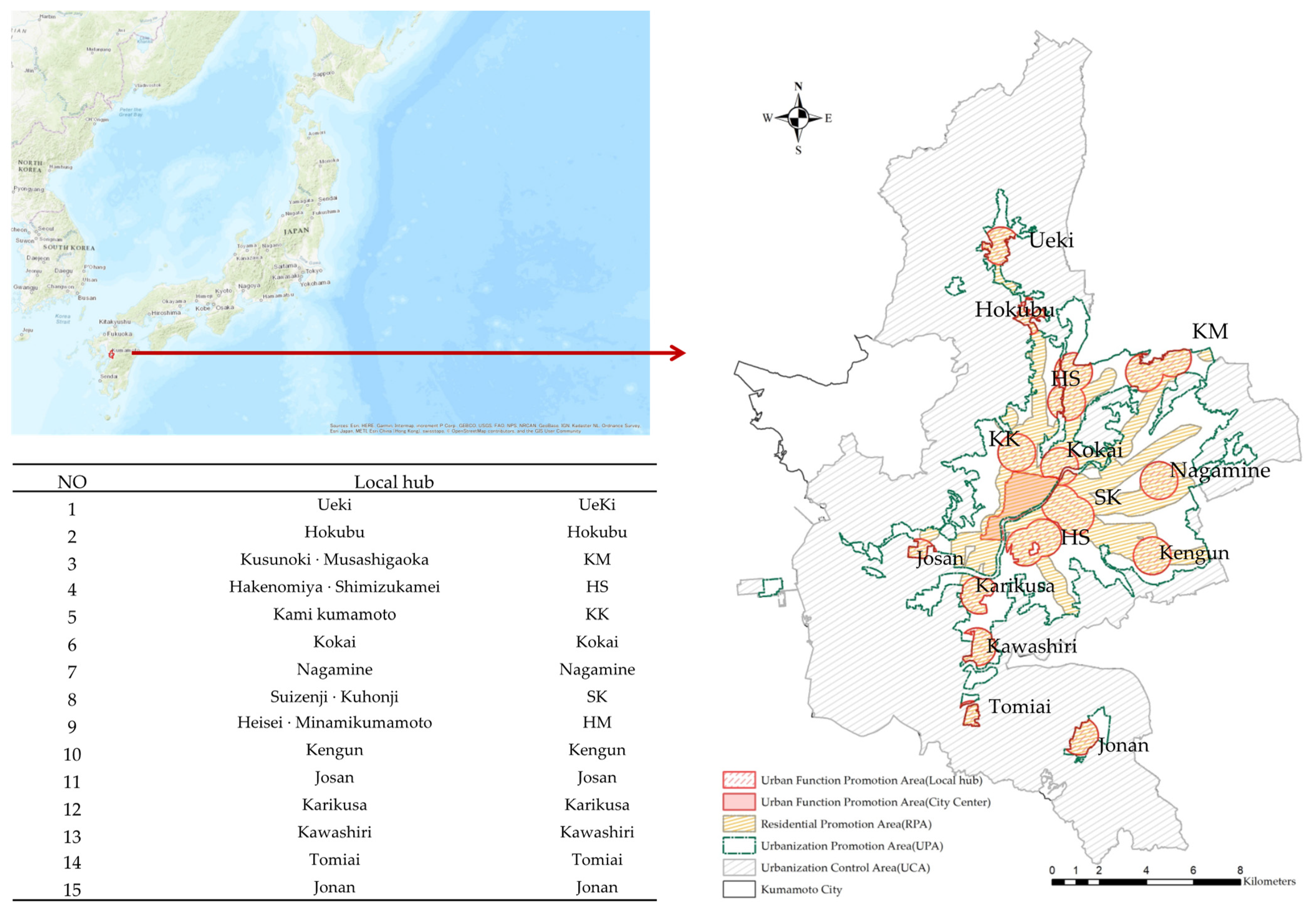
Kumamoto City, the capital of Kumamoto Prefecture, is in the center of Kyushu Island, at a latitude of 32°48 N and longitude of 103°42 E, covering an area of 390.32 km2 (Figure 1). From 1976 to 2008, urban construction land expanded 2.4 times [37]. Although the Urbanization Control Area (UCA) (Figure 1) has basically remained the same in recent years, the number of permitted developments has continued to increase, along with constant urban expansion. In response to the upcoming population decline and aging problem, the ‘Kumamoto City Master Plan-Regional Structure’, which was proposed in 2009 and formulated in 2014, projected the necessity of developing a compact city in Kumamoto City. After the 2016 Kumamoto earthquakes, the development of a disaster-resistant compact city was also proposed.
Kumamoto Compact City is a multinucleated urban structure, with 15 local hubs that are highly convenient and have well-developed functions, such as administration and commerce. These hubs are connected to the city center by public transportation, thus realizing a multinucleated interlocking city that is highly convenient and livable for everyone. These 15 local hubs and the central city area constitute the Urban Function Promotion Area (UFPA) (Figure 1). The Residential Promotion Area (RPA) (Figure 1) is where the population density is maintained within a certain area and usually has suitable facilities for daily life. Both the RPA and UFPA are in the Urbanization Promotion Area (UPA) (Figure 1). After the 2016 Kumamoto earthquakes, it became more urgent to use planning for inducing people to concentrate in safe and convenient residential and functional areas. In the post-earthquake urban master plan, Kumamoto City incorporated the concept of a disaster-proof multinuclear city, which will have a significant influence on the future direction of urban development and land use change in Kumamoto City.
Therefore, the prediction of land use change in Kumamoto City was divided into two scenarios. In Scenario I, the land use development model was assumed as an unconstrained development scenario without considering the impact of compact city policies and disasters, and only accounting for the influence of natural and socioeconomic factors. On the contrary, in Scenario II, the impact of compact development and disaster factors, such as the 2016 Kumamoto earthquakes and other disasters, were considered. The purpose is to contribute to urban disaster prevention planning and the management of Kumamoto City by comparing land use simulations in the two scenarios.
2.2. Land Use
The land use data were derived from the Kumamoto City Basic Survey and have three time periods: 2006, 2012, and 2018. The original data were in vector data format and converted to raster land use data with a resolution of 30 × 30 m using the polygon-to-raster function of ArcGIS 10.6. The original land use in the Kumamoto City Basic Survey was divided into 15 categories, and land classification was further organized into 10 categories according to this study’s requirements. Specific classifications and descriptions are presented in Table 1.
2.3. Driving Factors
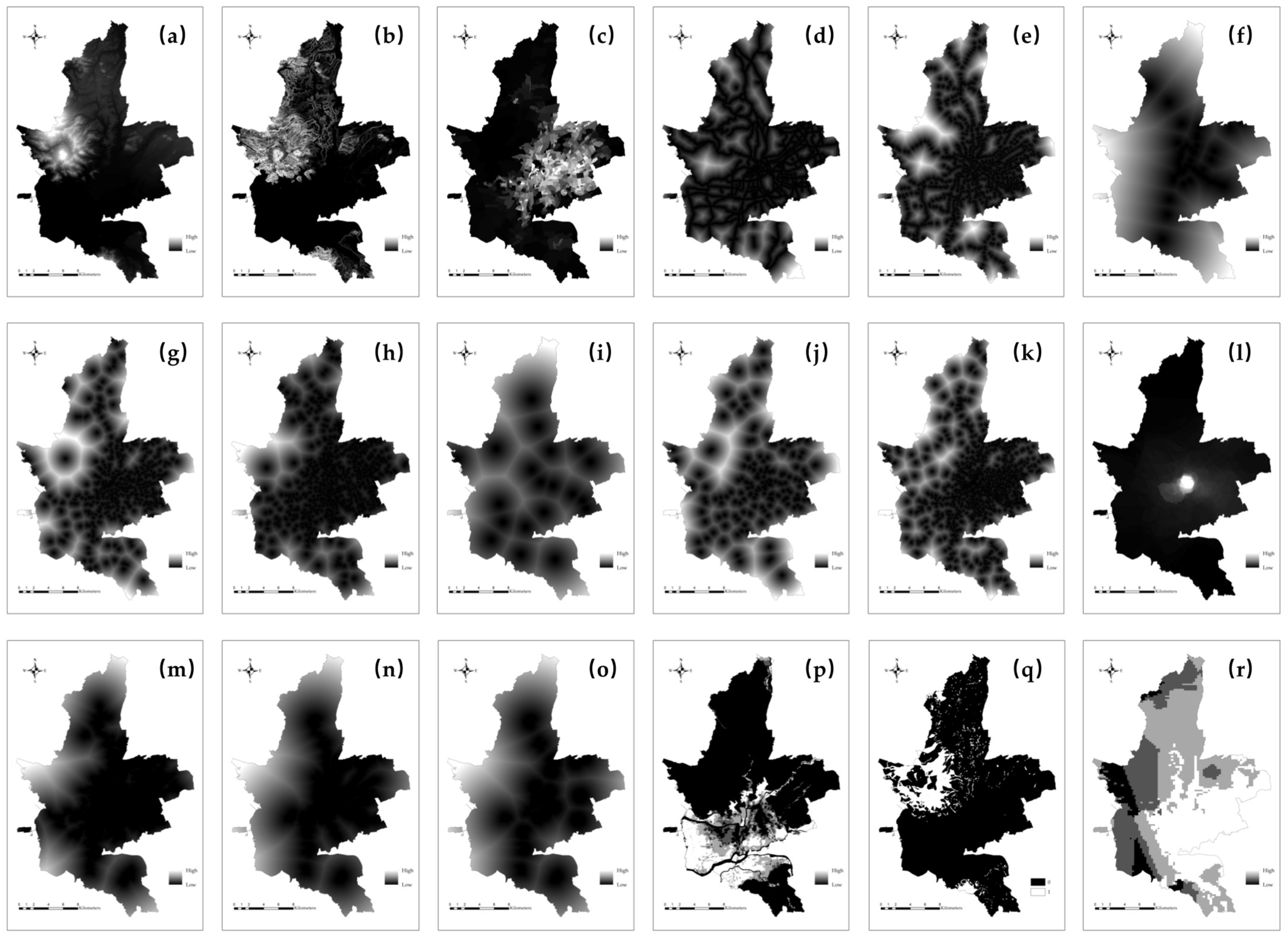
Land use change is the result of a combination of drivers, such as natural, socioeconomic, and policy factors [38,39]. Experts in land use change modeling have shown that some variables, such as elevation, slope, population, economic proxies, and distance from roads, are the main spatial indicators affecting land use changes [27]. The 18 driving factors in this study were divided into four categories: natural environmental factors (evaluation, slope, and aspect), socioeconomic factors (population density, distance to main roads, distance to railroad stations, land price, etc.), policy factors (distance to the UPA, distance to the RPA, distance to the UFPA), and disaster-related factors (floods, sediment, earthquakes) (Table 2). In addition, constrained factors were collected according to the needs of different scenario analyses. The simulation and prediction in the two scenarios used the corresponding driving factors.
DEM elevation data of natural environmental factors were obtained from the Geospatial Information Authority of Japan. Using the surface analysis tool, the slope was extracted from the DEM elevation data. As the original DEM data were 10 × 10 m, the data needed to be resampled and processed to 30 × 30 m to maintain consistency with the land use type data and lay the foundation for the subsequent simulation process. Resampling used the nearest neighbor method in the Resample tool of ArcGIS 10.6. Population data were obtained from the Basic Resident Register population of Kumamoto City, and the data included the total population in each basic unit block, which was converted to 30 × 30 m raster data after density calculation in ArcGIS 10.6. Main roads, rail stations, bus stops, and UPA were obtained from the Kumamoto City Basic Survey. Commercial and financial facilities, parks, schools, and disaster-related factors were collected from the National Land Numerical Information and Japan Seismic Hazard Information Station. Additionally, the RPA and UFPA were mapped using the criteria proposed in the Kumamoto City Master Plan. All distance variables in this study were calculated using the Euclidean Distance function in ArcGIS 10.6. The processing results are shown in Figure 2.
3. Methods
3.1. CA-RF Model
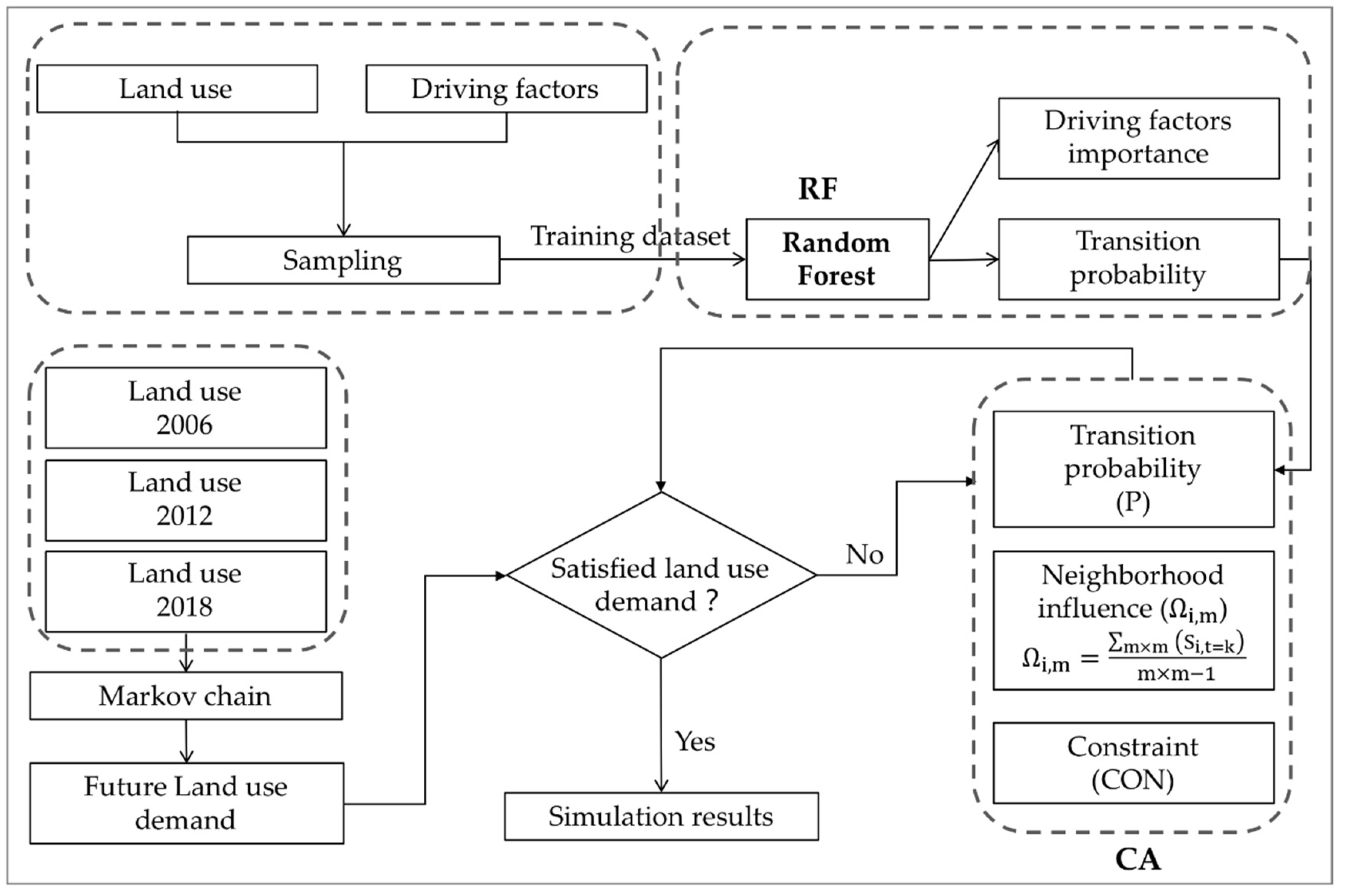
The CA-RF model is a coupled model of random forests and cellular automata that is used in land use change simulations. Each cell in the CA model, in general, has a transition rule that composes a function of how the cell decides its next state based on its previous state and its neighbors at a given moment [15,44]. The conceptual formula is expressed by the following Equation (1):
is the state of cell at time . is the state of cell at time , and is the transition function. is the overall transition probability. is the domain evaluation function, and denotes the neighborhood window size. A 3 × 3 size Moore neighborhood was used in this study. is the constraint of cell change, used to specify which cells can be changed, and is assigned to 1 if cell is available for development or change [15], and 0 otherwise. is the unknown random disturbance in the simulation that can produce more reliable results [45], where the parameter controls the size of the random variable, and is a random number falling in the range [0,1]. , can be calculated as follows:
In this study, the RF model was used to determine the transition probability of each cell, and the contribution of each driving factor could be obtained. We set up 100 decision trees to implement the random forest algorithm; additionally, the RF model was built with Scikit-learn [46]. The CA model was then used for land use change simulation and prediction. In addition, each land use demand, calculated by the Markov chain [47], was used to control the simulation iterations. Once the land demand was reached, the simulation process would stop. The simulation process of CA-RF was performed in Python in Anaconda Software. Figure 3 shows the workflow of the CA-RF model.
3.2. Validation
The kappa coefficient is usually used in the assessment of the accuracy of land use simulation models [48]. Its value can be used to determine the reliability between the observed consistency and chance consistency [49,50]. In this study, the 2012 and 2018 land use results simulated by the two scenarios were compared with the observed 2012 and 2018 land use to validate the prediction consistency. The kappa coefficient was calculated as follows:
where is the proportion of actual and simulated land use cells that are identical (correct simulated proportion); is the proportion of land use simulated cells to the actual raster in the random case (simulated proportion under the expectation of random conditions); , , and denote the total number of current land use cells, the number of simulated correct land use cells, and the number of land use classifications, respectively. Kappa takes values in the range of 0–1.
4. Results
4.1. Simulation and Validation
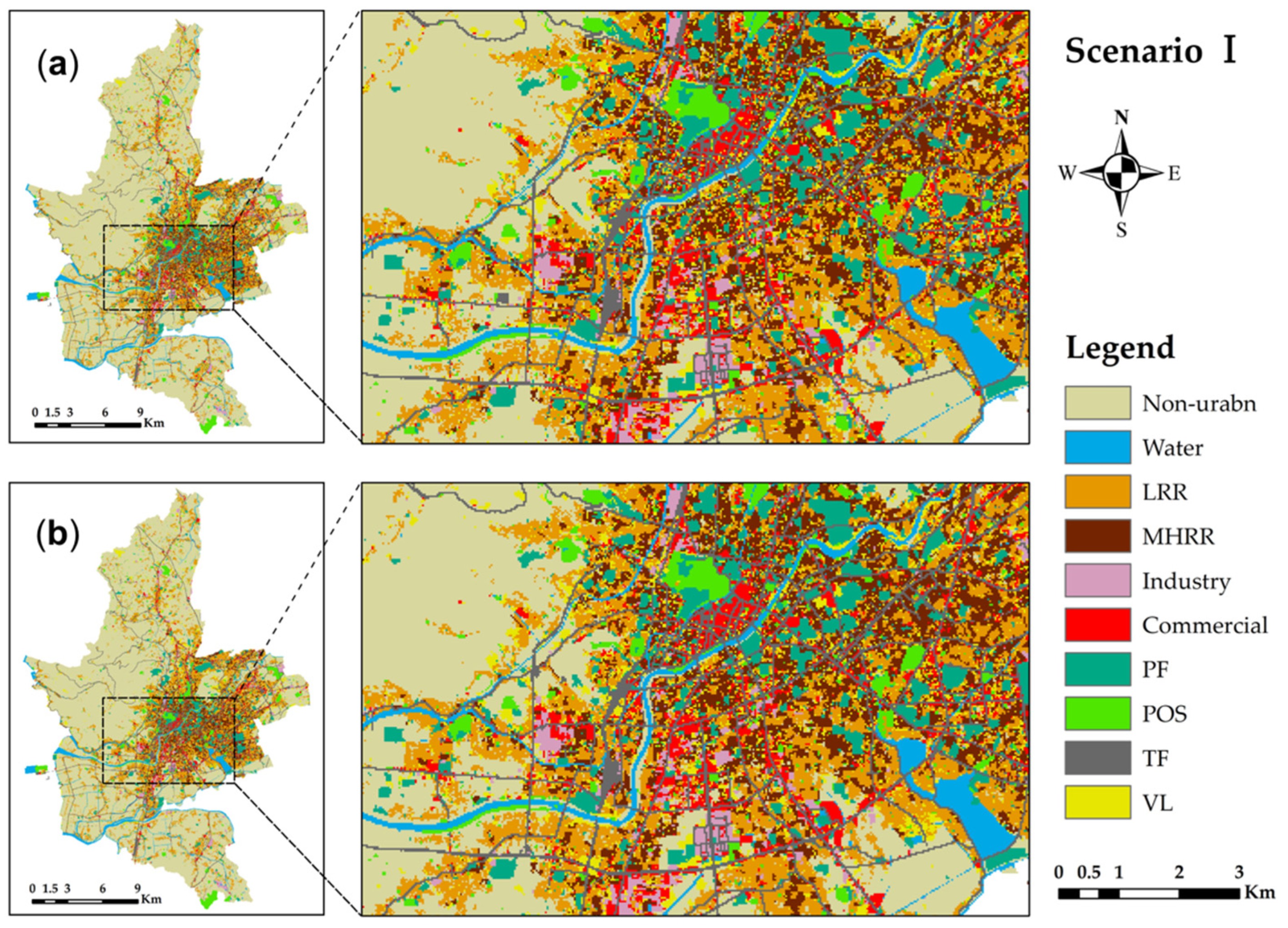
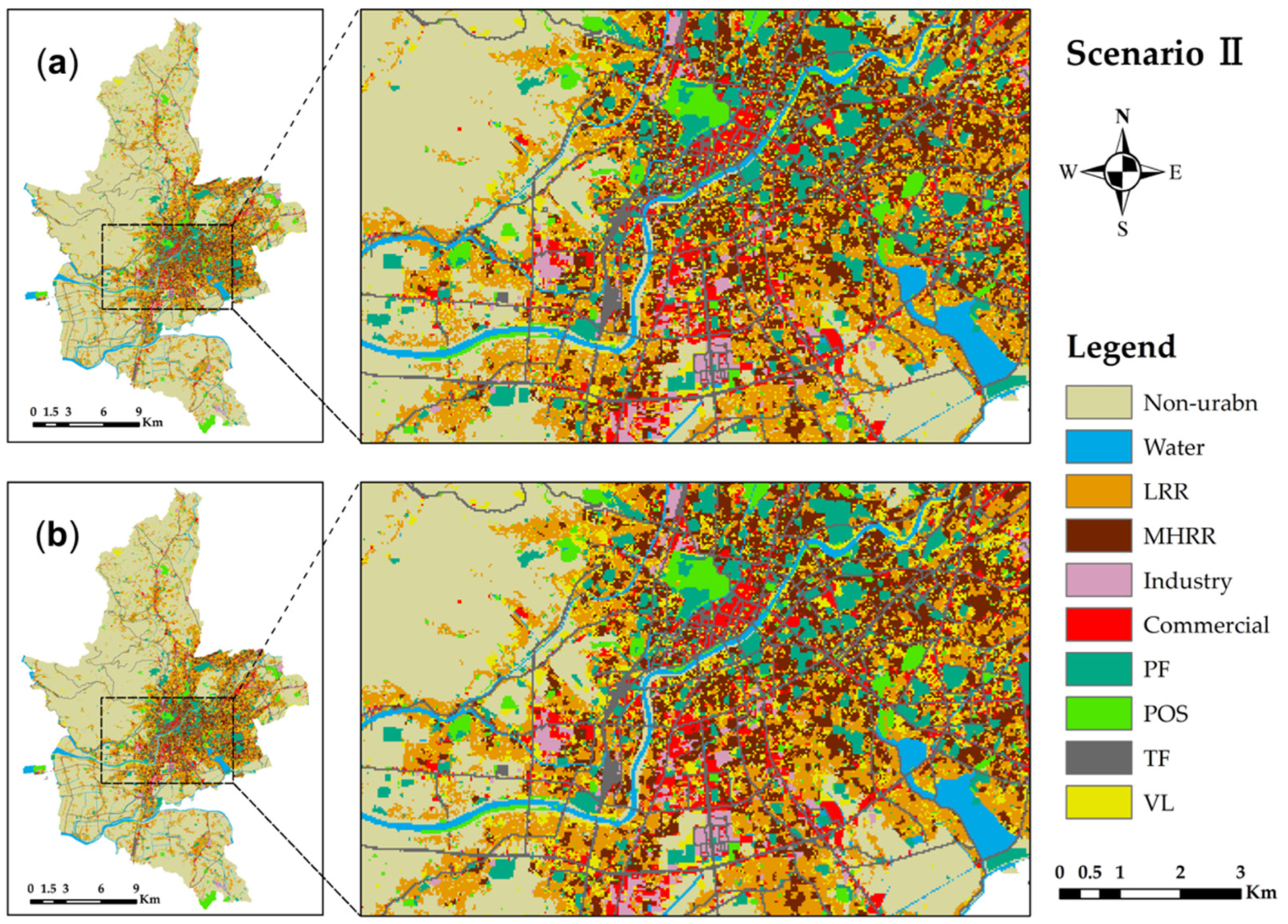
This study simulated the urban space of Kumamoto City in 2012 and 2018 according to the constructed model in two scenarios. The spatial simulation results show that the simulation results (Figure 4b and Figure 5b) and observed land use (Figure 4a and Figure 5a) generally have a high consistency. The overall accuracy of Scenario I was 96.40%, and the kappa coefficient was 0.944, while the accuracy of Scenario II was 96.35%, with a kappa coefficient of 0.943. Therefore, we believe that this model is suitable for predicting future urban land use changes in Kumamoto City.
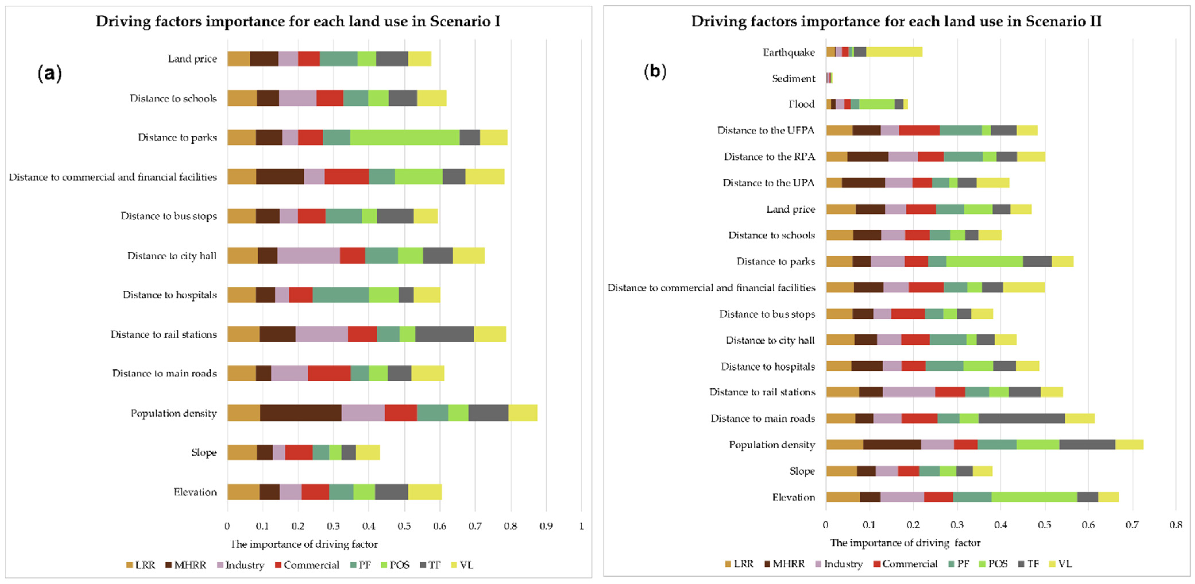
According to the random forest algorithm, the driving factors’ contribution for each land use can be assessed. The driving factors’ importance in Scenario I is illustrated in Figure 6a. In low-rise residential (LRR), each factor is of approximately equal importance, with population density and distance to rail stations being the most significant factors. For medium high-rise residential (MHRR), the essential factors are population density and distance to commercial and financial facilities. For commercial land, the distance to commercial and financial facilities and the distance to main roads are vital. The distance to commercial and financial facilities and the distance to main roads and railway stations are the key factors affecting the formation of vacant land (VL).
Figure 6b shows that, in Scenario II, the distances from medical, commercial, and financial facilities related to urban life and the distances from certain transportation location factors (bus and railway stations) are of approximately equal importance for LRR changes, with population density remaining the most important factor. In addition to population density, distances to health, commercial, and financial facilities associated with urban life are attractive, and urban planning factors, such as distance to the UPA and distance to the RPA, also play an important role. The distance to the UFPA is the most significant factor affecting commercial and public facilities. In addition, seismic intensity was the most significant factor for VL.
4.2. Scenario I
Table 3 shows the observed land use area changes from 2006 to 2012 and the simulated changes in Scenario I from 2018 to 2030. In this scenario, we assume that urban development is basically unrestricted, predict urban land development in 2018, 2024, and 2030, and calculate the area changes of each land use. The results show that the rate of urban land is steadily increasing, and the overall decrease in non-urban land remains stable. In terms of urban land, the area of LRR has the largest increase, growing to 266.49 ha, 261.54 ha, and 256.32 ha by 2018, 2024, and 2030, respectively. VL and MHRR also show high growth rates. It is worth noting that these growth rates are declining each year, similar to industrial land and public open space (POS). However, commercial and transportation facility (TF) land shows an increasing trend each year. The area of water bodies remains unchanged.
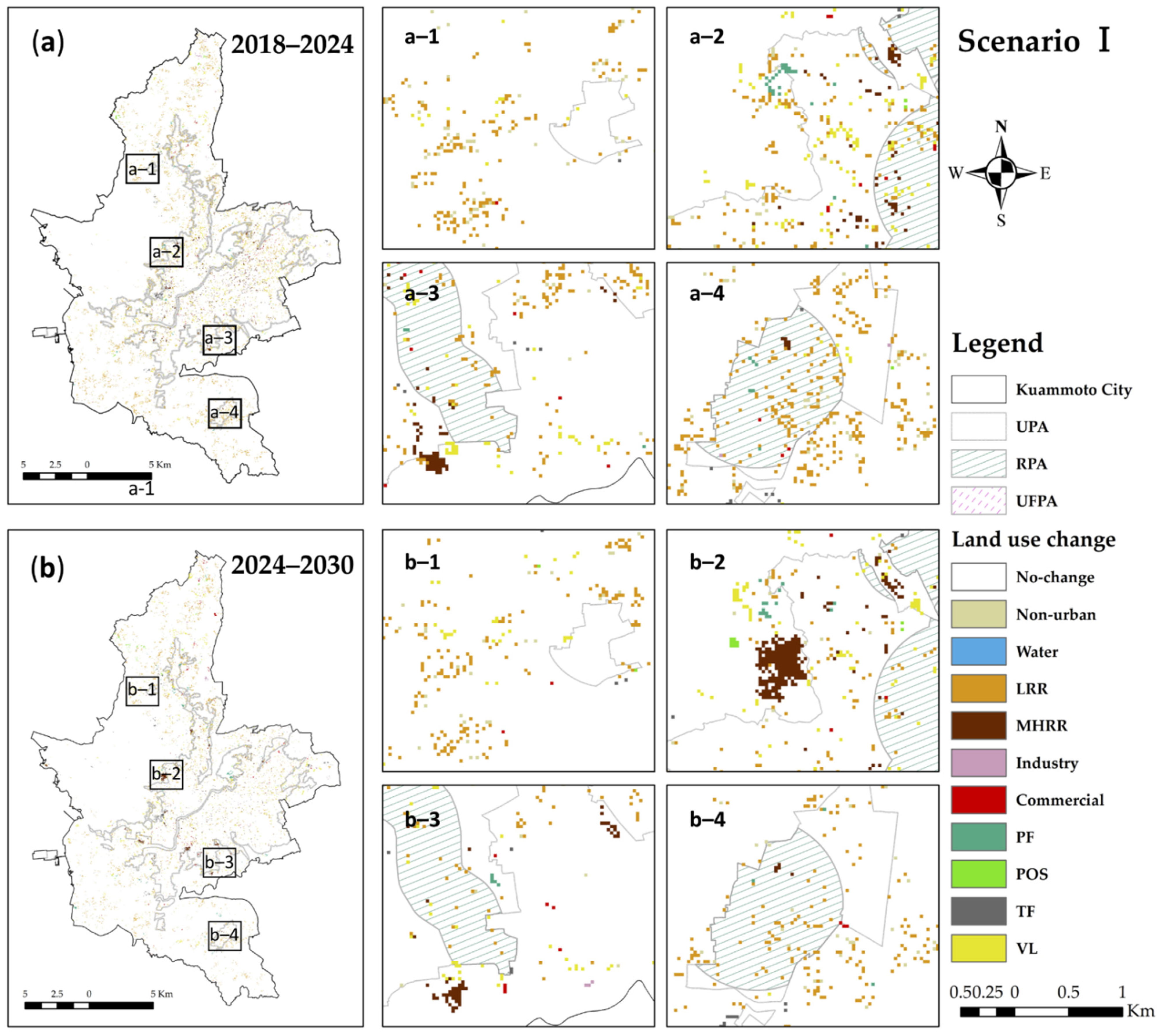
From the perspective of spatial change, the distribution of urban land change is shown in Figure 7. A large amount of future LRR growth is mainly distributed in the periphery of the UPA, as shown in Figure 7(a–1), but also in the UFPA area, which is further away from the central area (as shown in Figure 7(a–4)). This trend of LRR growth will continue from 2018–2024 (as shown in Figure 7(a–1,a–4)) to 2024–2030 (as shown in Figure 7(b–1,b–4)). The MHRR, on the other hand, is mainly distributed in the outer area near the UPA boundary, with small areas of concentration appearing in 2018–2024, as shown in Figure 7(a–2,a–3), and more areas of concentration in 2024–2030, as shown in Figure 7(b–2,b–3). The growth of VL is mainly distributed inside the UPA.
4.3. Scenario II
The growth of land use changes was also calculated for the observed changes in land use area from 2012 to 2018 and the simulated changes in Scenario II from 2024 to 2030 (Table 4). In this scenario, we assume that urban development is influenced and constrained by urban planning policies while considering the impact of disaster factors. The results show that the rate of urban expansion decreases significantly. Non-urban land will reduce from 440.82 ha in 2018 to 189.99 ha in 2030. In terms of urban land, the VL area increased the most in 2018 and 2024, with 175.41 ha and 170.46 ha, respectively. However, by 2024, the area of VL is basically the same as that in 2024, with an increase of only 2.34 ha. On the contrary, LRR and MHRR maintain a relatively stable growth. Furthermore, industrial land, PF, and POS show a trend of slow growth (from 2018 to 2024) or even negative growth (from 2024 to 2030).
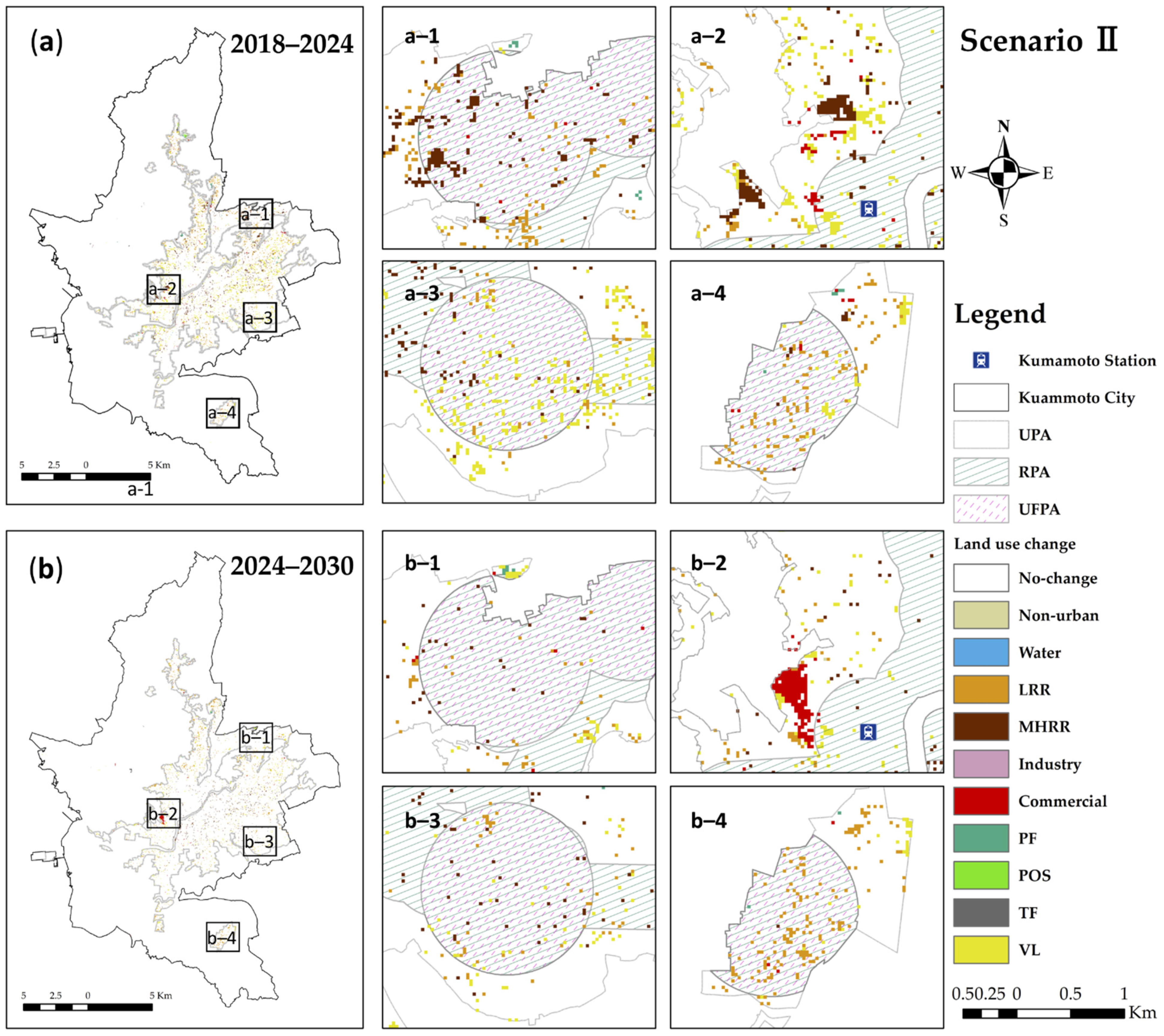
The spatial distribution of urban land use changes is shown in Figure 8. With constraints, urban land use growth is widely distributed within the UPA. From 2018 to 2030, future LRR growth mainly appears within the borderline areas of the UPA and some UFPA areas far from the central area, as shown in Figure 8(a–4,b–4). MHRR is also widely distributed, with more growth in the central area, but more dispersed. From 2018 to 2024, concentrations appear in some UFPA areas (e.g., Figure 8(a–1)), but in this region, there is no significant growth from 2024 to 2030 (e.g., Figure 8(b–1)). More growth concentrations occur between UPA and FPA in 2018–2024, as shown in Figure 8(a–2). In 2024–2030, urban land use for growth concentration in this area is commercial, as shown in Figure 8(b–2). Growth in VL is widely distributed within the UPA in 2018–2024, as shown in Figure 8(a–3), while in 2024–2030, the growth decreases (Figure 8(b–3)). To gain a better understanding of land use change inside urban planning areas, we calculated the UPA, RPA, and UFPA.
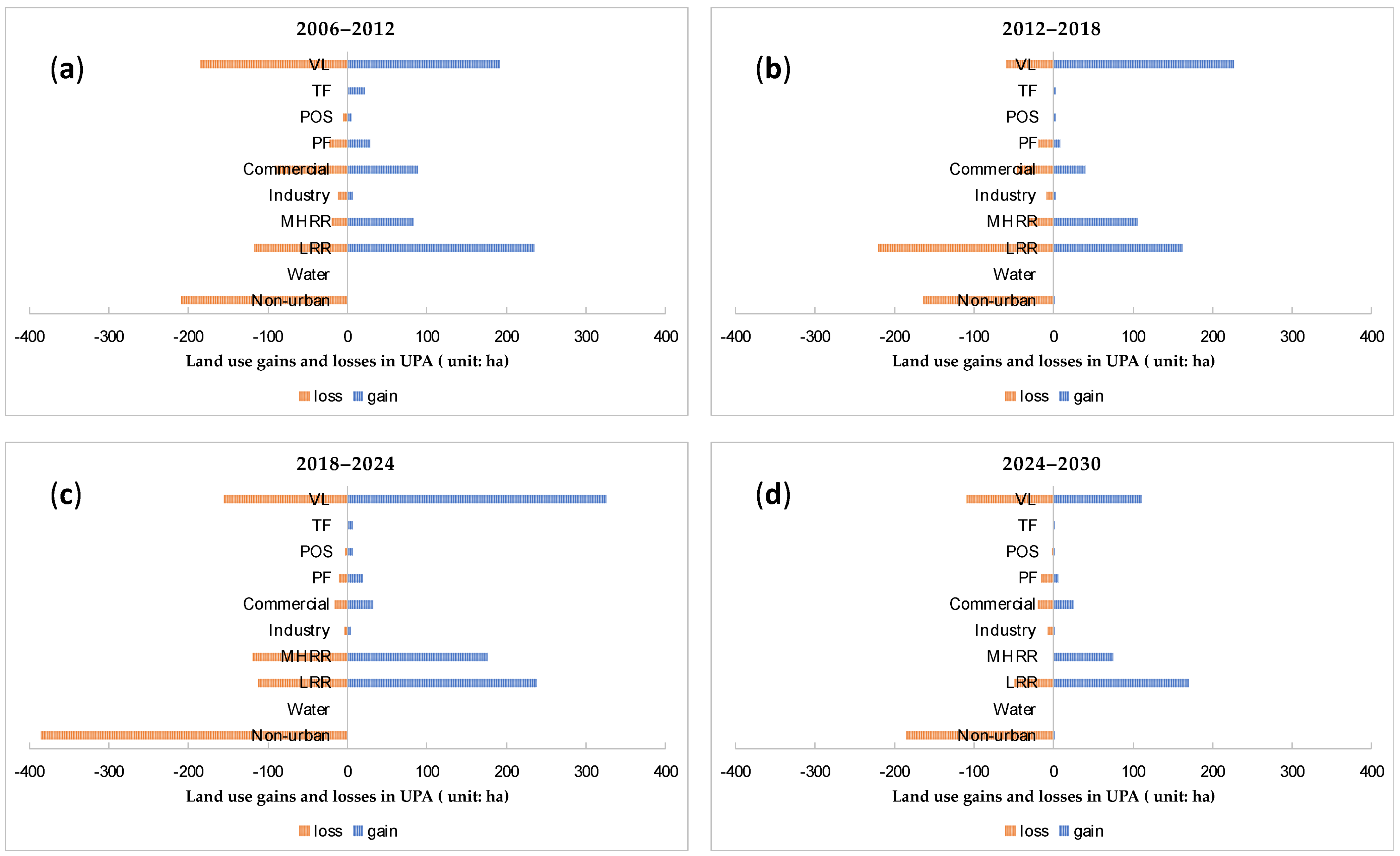
Figure 9 shows the gains and losses in the UPA between 2006 and 2030. In the first period (2006–2012), LRR had the highest (235.08 ha) gains, followed by VL (192.42 ha). Non-urban areas had the highest losses (209.43 ha), followed by VL (185.43 ha). In the second period (2012–2018), VL gained the most (227.25 ha), while LRR was the land use type with the greatest losses (220.41 ha). In the third period (2018–2024), the result of the prediction shows that VL will gain the most (326.16 ha). Meanwhile, the gains of LRR and MHRR also indicate post-disaster recovery. In the fourth period (2024–2030), the transition between different types of land use decreases. LRR will have the highest gains (170 ha), followed by VL (111.69 ha) and MHRR (74.52 ha). However, the losses and gains of VL will reach a balanced state. Non-urban land maintains high losses over the four periods.
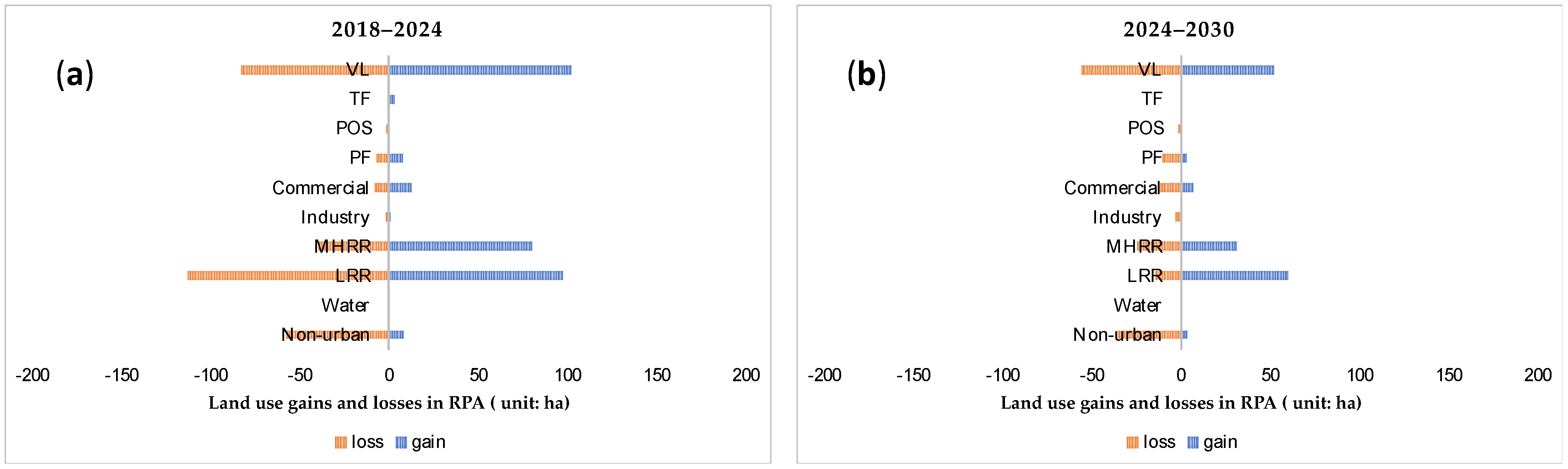
Figure 10 shows the gains and losses in the RPA between 2006 and 2030. The overall gains and losses were similar to those in the UPA. In the first period (2006–2012), VL had the highest gains (122.85 ha), followed by LRR (111.15 ha). During this period, the highest loss was also that of VL (98.01 ha), but the overall gains were greater than the losses. In the second period (2012–2018), VL continued to gain the most (122.58 ha), and LRR was the land use type with the greatest loss (120.96 ha). In the third period (2018–2024), the prediction result shows that VL will have the greatest gain (167.31 ha), followed by MHRR (110.33 ha) and LRR (104.76 ha). In the fourth period (2024–2030), VL will have the highest gains (106.29 ha), followed by LRR (72.81 ha) and MHRR (48.24 ha). During the four periods, the losses of non-urban land in the RPA are maintained at a relatively high level. VL, LRR, and MHRR always maintain high gains and losses, and the underlying gains are greater than the losses (except for LRR between 2012 and 2018).
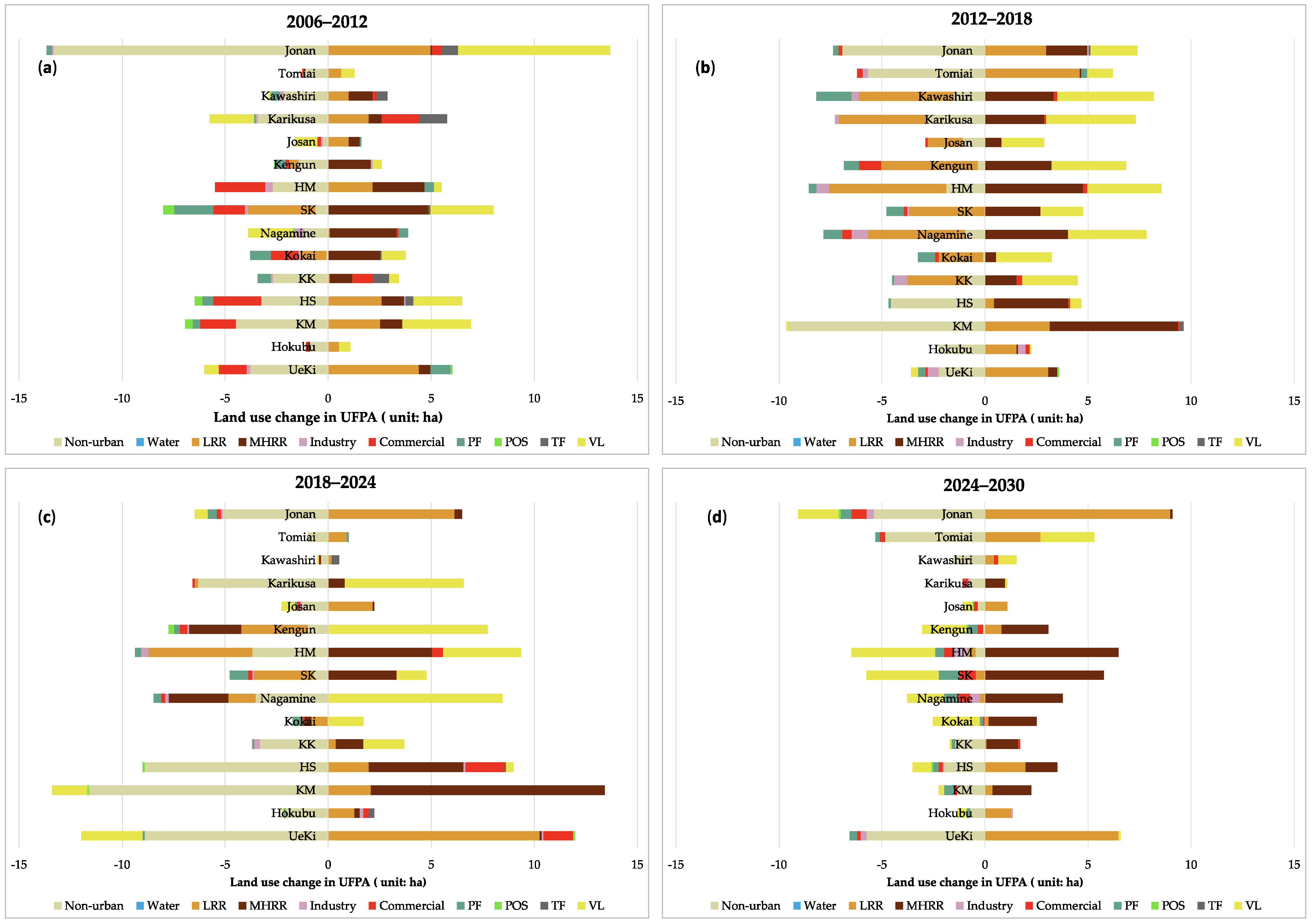
Figure 11 shows the changes in each land use type in 15 local hubs between 2006 and 2030. In the first period (2006–2012) (Figure 11a), LRR increased more in Jonan, Ueki, KM, and KK, while it decreased in SK and Kokai. MHRR increased significantly in local hubs, such as SK, Nagamine, Kokai, HM, and Kengun. VL in Jonan, SK, KM, and HS showed a relatively large increase. Among the 15 local hubs, Jonan had the largest change, with non-urban areas decreasing by 13.32 ha, VL and LRR increasing by 7.38 ha and 4.95 ha, respectively. Local hubs, such as Hokubu, showed the least change. In general, during this period, there were three types of development patterns. The first is the local hubs far away from the city center represented by Jonan, Ueki, and KM, showing a rapid change pattern, which can be evidenced by the rapid growth of LRR and the decrease in non-urban areas. The second is the rapid growth of MHRR near the city center represented by SK, Nagamine, and Kokai. The third is the low-speed change pattern far away from the city center represented by Tomiai and Hokubu.
In the second period (2012–2018) (Figure 11b), land use changes in the KM were the most significant. Non-urban land use decreased by 9.54 ha, while LRR and MHRR increased by 3.15 ha and 6.21 ha, respectively. There are two types of development. One is the continuous increase in LRR represented by Jonan, Tomiai, and Ueki. The other is the decrease in LRR and the increase in MHRR and VL, such as in the case of HM and Nagamine.
In the third period (2018–2024) (Figure 11c), the predicted results indicate significant changes in local hubs, such as KM, Ueki, HS, and Jonan, with an increase in MHRR in KM and HS, and an increase in LRR in Ueki and Jonan. In contrast, local hubs such as Kengun and Nagamine, which are located near the epicenter, show a continuous growth in VL.
In the fourth period (2024–2030) (Figure 11d), two main patterns are evident. The local hubs outside the city center are predicted to maintain a relatively rapid growth pattern of LRR, such as Jonan and Ueki. The growth in MHRR near the city center, such as in HM and SK, is significant. In these areas, in contrast, vacant land is declining.
5. Discussion
Scenario II added driving factors related to urban planning and natural disasters compared to Scenario I. The random forest provided a good indication of the importance of the driving factors. Comparing the results of the two scenarios shows that the importance of the driving factors that affect each land use could change. For example, the most important driving factor for commercial land is the distance to commercial and financial facilities in Scenario l, shifting to the distance to the UFPA in Scenario II. The UFPA is an area where various types of facilities (e.g., commercial, financial, medical) are promoted to develop in Kumamoto City, and it contains the city center and the local hubs. The city center has the attraction of commercial investment, and many studies [13,51,52,53] have taken it as an important factor influencing land use change; a previous study by Zhang et al. [26] could draw a similar conclusion that the distance to the city center has the greatest impact on commercial land. The driving factor with the highest contribution to VL is the distance to commercial and financial facilities in Scenario I, changing to an earthquake-related factor in Scenario II. This indicates that the 2016 Kumamoto earthquakes had an important impact on land vacancy. In both scenarios, in addition to the population density factor, facilities related to residential life and transportation factors are important factors in residential land use change [26]. Therefore, in order to accurately reflect the change in urban land use, the selection of driving factors is important.
Urban policies were often used as limiting factors (urban development restriction areas, farmland protection areas, etc.) in the previous studies [11,27,54]. In this study, combining the characteristics of urban planning policies in Japan, the planning promotion development area was used as a driving factor, and the restriction area was used as a restriction factor. The UPA, RFA, and UFPA, as development promotion areas, show a significant influence on residential, commercial, etc. RFA is a residential-induced area, attracting people to live in this area for the convenience of living. In addition, the UFPA is an urban function-induced area, where various facilities are concentrated. Due to these characteristics, the urban planning areas are an important factor that should be introduced in this study to enhance the simulation of intra-urban land use. In addition, for Japan, as a disaster-prone country, disasters are a factor to be taken into account.
The scenario-based results show that urban planning policies incorporated into land use simulation models play an essential role in guiding the sustainable development of Kumamoto City. The changes of each land use type in the city vary remarkably between the two scenarios, the spatial distribution of which is also different. In Scenario I, each land use type in Kumamoto City shows a spatially disordered development. However, there is also some concentration growth in 2024–2030. It can be seen that the concentration-generating zones are basically MHRR, but they are found in the outside boundary areas of the UPA. For the overall urban development, it remains a continuous urban expansion, which contradicts Kumamoto’s policy of compact urban development. These areas are close to the UPA, relatively more convenient than the outer urban areas, and have good development conditions and high development attractiveness. In Scenario II, we considered the impact of various disasters in Kumamoto City and urban planning factors, and the results indicate that the development is more compact than Scenario I. The growth shows continuity and correlation. For example, in Figure 8(a–2), from 2018 to 2024, a large number of MHRR areas appear, and by 2024–2030(Figure 8(b–2)), a significant concentration of commercial areas appears around these MHRR lands. We found that the growth in this area may be attributed to the development of Kumamoto Station, whose renewal development after the opening of the Shinkansen in 2012 has led to the development of the surrounding area. Compact city development in Japan also relies on transportation stations; therefore, we believe that this predicted result is somewhat realistic. In addition, we found that the residential development within some UFPA areas that are far from the city center may be different from that of the central area. Its residential land induction in these areas could mainly focus on promoting LRR due to the low population density (Figure 8(a–4,b–4)).
In addition, overall, land use changes in land use within each urban planning area for Scenario I are less than those in Scenario II. Within the UPA, the losses of non-urban land use in Scenario I from 2018 to 2024 (Figure A1a in Appendix A) are significantly less than those in Scenario II (Figure 9d), indicating that Scenario II still requires a certain amount of new land to promote development during this period. In 2018–2024, the gains of LRR are basically the same for both scenarios (Figure A1b and Figure 9d). However, Scenario I will have more losses, which may be due to more out-migration to the suburbs in the case of unrestricted development. At the same time, it is noticed that there is a very significant increase in VL change for Scenario II during this period, which may be attributed to the 2016 Kumamoto earthquakes, which caused numerous buildings to collapse and rendered the land vacant. In 2024–2030, there is no significant difference in the development of the two scenarios. Moreover, each land use shows fewer changes than the previous period, with a slower development speed. The comparison of Scenario I (Figure A2) and Scenario II (Figure 10c,d) in the RPA shows that similar results to the UPA can be obtained. In the local hub of the UFPA, the VL of Nagamine and Kengun shows a continuous growth trend from 2012 to 2024 (Figure 11b,c) in Scenario II. These local hubs are close to the epicenter of the 2016 Kumamoto earthquakes with high seismic intensity. The local hubs such as Ueki, which are farther away from the city center, are also distant from the epicenter, and they have faster residential growth from 2012 until 2024. Since Scenario I does not consider the effects of disasters, there is no significant growth in VL from 2018 to 2024 (Figure A3a). From 2024 to 2030, the growth trend slows down in both scenarios. However, it can be seen that the local hubs in Scenario I (Figure A3b) are mainly the growth of LRR, while Scenario II (Figure 11d) mainly shows the growth of MHRR, especially in local hubs closer to the city center, such as HM and SK. The results of the UPA, RPA, and UFCA show that the development of urban land use is guided by urban planning, and MHRR has significant growth and a trend of compact development. Meanwhile, the earthquake factor has a great impact on the formation of VL in these areas, especially in the areas near the epicenter, which should be re-evaluated in terms of post-disaster reconstruction and whether it is reasonable for these areas to be used for residential promotion.
This study also has some limitations, such as a certain amount of established development settlements within the UCA. Within these development settlements, a certain level of development is allowed, and this study restricted all development within the UCA, which may affect the accuracy of the model to some extent. In addition, Japan is already an aging society [55], and population decline has become a problem for many cities. To solve the decreasing population in the future, Japanese cities have proposed compact city policies to control urban growth [56]. In the future land use simulation within Japanese cities, the context of a declining population needs to be considered. This study only integrated the compact city policy into the model and has not yet included the expected future population decline data. Future studies can use the cohort population projection data provided by the Japanese government to carry out predictions of intra-urban land use changes, especially changes in residential areas, and the development of empty houses. Whether urban development will show a corresponding shrinking in the face of population decline is also a direction for future research.
6. Conclusions
In this study, we predicted future urban land use changes in Kumamoto City by combining random forest and cellular automata models. The validation of the simulation results under two scenarios in 2012 and 2018 showed that the RF-CA model is suitable for predicting future intra-urban land use change. The specific development policies and disaster prevention requirements of Japanese cities were fully considered, further validating the effectiveness of the RF-CA model for intra-urban land use changes under multiple scenarios. Moreover, this study also enriched the application scenarios of the RF-CA model.
In Scenario I with unconstrained development conditions, future land use (other than water and non-urban land) in Kumamoto City will show a steady growth trend. With this growth trend, Kumamoto urban development will continue to expand outside the UPA. Under the intervention of urban planning and considering the impact of disasters, although the area of urban land will continue to grow in general, it will show a trend of slow and compact growth, and there will be some relatively distinct growth centers. Moreover, some urban land uses, such PF and industry, show negative growth in the future. Future development of Kumamoto City may move towards shrinking. This is worthy of reference to provide urban planners and decision makers with the direction of future urban development.
Author Contributions
Conceptualization, Hang Liu, Riken Homma, Qiang Liu, and Congying Fang; methodology, Hang Liu, Riken Homma, Qiang Liu, Congying Fang; software, Hang Liu; validation, Hang Liu, Qiang Liu; formal analysis, Hang Liu; investigation, Hang Liu, Qiang Liu, Congying Fang; resources, Hang Liu, Riken Homma; data curation, Hang Liu, Riken Homma; writing—original draft preparation, Hang Liu, Riken Homma, Qiang Liu, Congying Fang; writing—review and editing, Hang Liu; visualization, Hang Liu; supervision, Riken Homma; project administration, Hang Liu, Riken Homma; funding acquisition, Riken Homma, Hang Liu. All authors have read and agreed to the published version of the manuscript.
Funding
This research received no external funding.
Data Availability Statement
The datasets in this study are publicly available, summarized and referenced in Table 2.
Conflicts of Interest
The authors declare no conflict of interest.
Appendix A
Figure A1.
Gains and losses in the UPA between 2018 and 2030 in Scenario I: (a) gains and losses between 2018 and 2024; (b) gains and losses between 2024 and 2030.
Figure A1.
Gains and losses in the UPA between 2018 and 2030 in Scenario I: (a) gains and losses between 2018 and 2024; (b) gains and losses between 2024 and 2030.

Figure A2.
Gains and losses in the RPA between 2018 and 2030 in Scenario I: (a) gains and losses between 2018 and 2024; (b) gains and losses between 2024 and 2030.
Figure A2.
Gains and losses in the RPA between 2018 and 2030 in Scenario I: (a) gains and losses between 2018 and 2024; (b) gains and losses between 2024 and 2030.

Figure A3.
Land use change in the UFPA between 2018 and 2030 in Scenario I: (a) land use change between 2018 and 2024; (b) land use change between 2024 and 2030.
Figure A3.
Land use change in the UFPA between 2018 and 2030 in Scenario I: (a) land use change between 2018 and 2024; (b) land use change between 2024 and 2030.

References
- Gu, W.; Guo, J.; Fan, K.; Chan, E.H.W. Dynamic Land Use Change and Sustainable Urban Development in a Third-Tier City within Yangtze Delta. Procedia Environ. Sci. 2016, 36, 98–105. [Google Scholar] [CrossRef] [Green Version]
- Musakwa, W.; Niekerk, A.V. Implications of Land Use Change for the Sustainability of Urban Areas: A Case Study of Stellenbosch, South Africa. Cities 2013, 32, 143–156. [Google Scholar] [CrossRef]
- Zhang, H.; Uwasu, M.; Hara, K.; Yabar, H. Land Use Change Patterns and Sustainable Urban Development in China. J. Asian Archit. Build. Eng. 2010, 9, 131–138. [Google Scholar] [CrossRef]
- Karakus, C.B.; Cerit, O.; Kavak, K.S. Determination of Land Use/Cover Changes and Land Use Potentials of Sivas City and Its Surroundings Using Geographical Information Systems (GIS) and Remote Sensing (RS). Procedia Earth Planet. Sci. 2015, 15, 454–461. [Google Scholar] [CrossRef] [Green Version]
- Verburg, P.H.; Schot, P.P.; Dijst, M.J.; Veldkamp, A. Land Use Change Modelling: Current Practice and Research Priorities. GeoJournal 2004, 61, 309–324. [Google Scholar] [CrossRef]
- Yang, Y.; Bao, W.; Liu, Y. Scenario Simulation of Land System Change in the Beijing-Tianjin-Hebei Region. Land Use Policy 2020, 96, 104677. [Google Scholar] [CrossRef]
- Aburas, M.M.; Ahamad, M.S.S.; Omar, N.Q. Spatio-Temporal Simulation and Prediction of Land-Use Change Using Conventional and Machine Learning Models: A Review. Environ. Monit. Assess. 2019, 191, 205. [Google Scholar] [CrossRef]
- Mustafa, A.; Cools, M.; Saadi, I.; Teller, J. Coupling Agent-Based, Cellular Automata and Logistic Regression into a Hybrid Urban Expansion Model (HUEM). Land Use Policy 2017, 69, 529–540. [Google Scholar] [CrossRef] [Green Version]
- Chang-Martínez, L.A.; Mas, J.-F.; Valle, N.T.; Torres, P.S.U.; Folan, W.J. Modeling Historical Land Cover and Land Use: A Review FromContemporary Modeling. ISPRS Int. J. Geo-Inf. 2015, 4, 1791–1812. [Google Scholar] [CrossRef] [Green Version]
- Qian, Y.; Xing, W.; Guan, X.; Yang, T.; Wu, H. Coupling Cellular Automata with Area Partitioning and Spatiotemporal Convolution for Dynamic Land Use Change Simulation. Sci. Total Environ. 2020, 722, 137738. [Google Scholar] [CrossRef] [PubMed]
- Zhou, L.; Dang, X.; Sun, Q.; Wang, S. Multi-Scenario Simulation of Urban Land Change in Shanghai by Random Forest and CA-Markov Model. Sustain. Cities Soc. 2020, 55, 102045. [Google Scholar] [CrossRef]
- Xing, W.; Qian, Y.; Guan, X.; Yang, T.; Wu, H. A Novel Cellular Automata Model Integrated with Deep Learning for Dynamic Spatio-Temporal Land Use Change Simulation. Comput. Geosci. 2020, 137, 104430. [Google Scholar] [CrossRef]
- Sun, J.; Zhang, L.; Peng, C.; Peng, Z.; Xu, M. CA-Based Urban Land Use Prediction Model: A Case Study on Orange County, Florida, U.S. J. Transp. Syst. Eng. Inf. Technol. 2012, 12, 85–92. [Google Scholar] [CrossRef]
- Tayyebi, A.; Delavar, M.R.; Yazdanpanah, M.J.; Pijanowski, B.C.; Saeedi, S.; Tayyebi, A.H. A Spatial Logistic Regression Model for Simulating Land Use Patterns: A Case Study of the Shiraz Metropolitan Area of Iran. In Advances in Earth Observation of Global Change; Chuvieco, E., Li, J., Yang, X., Eds.; Springer: Dordrecht, The Netherlands, 2010; pp. 27–42. ISBN 978-90-481-9085-0. [Google Scholar]
- Feng, Y.; Liu, Y.; Tong, X. Comparison of Metaheuristic Cellular Automata Models: A Case Study of Dynamic Land Use Simulation in the Yangtze River Delta. Comput. Environ. Urban Syst. 2018, 70, 138–150. [Google Scholar] [CrossRef]
- Gharaibeh, A.; Shaamala, A.; Obeidat, R.; Al-Kofahi, S. Improving Land-Use Change Modeling by Integrating ANN with Cellular Automata-Markov Chain Model. Heliyon 2020, 6, e05092. [Google Scholar] [CrossRef]
- Li, T.; Li, W. Multiple Land Use Change Simulation with Monte Carlo Approach and CA-ANN Model, a Case Study in Shenzen, China. Environ. Syst. Res. 2015, 4, 1–10. [Google Scholar] [CrossRef] [Green Version]
- Qiang, Y.; Lam, N.S.N. Modeling Land Use and Land Cover Changes in a Vulnerable Coastal Region Using Artificial Neural Networks and Cellular Automata. Environ. Monit. Assess. 2015, 187, 57. [Google Scholar] [CrossRef] [PubMed]
- Li, X.; Yeh, A.G.-O. Neural-Network-Based Cellular Automata for Simulating Multiple Land Use Changes Using GIS. Int. J. Geogr. Inf. Sci. 2002, 16, 323–343. [Google Scholar] [CrossRef]
- Liu, Y.; Feng, Y. Simulating the Impact of Economic and Environmental Strategies on Future Urban Growth Scenarios in Ningbo, China. Sustainability 2016, 8, 1045. [Google Scholar] [CrossRef] [Green Version]
- Mustafa, A.; Rienow, A.; Saadi, I.; Cools, M.; Teller, J. Comparing Support Vector Machines with Logistic Regression for Calibrating Cellular Automata Land Use Change Models. Eur. J. Remote Sens. 2018, 51, 391–401. [Google Scholar] [CrossRef]
- Yang, Q.; Li, X.; Shi, X. Cellular Automata for Simulating Land Use Changes Based on Support Vector Machines. Comput. Geosci. 2008, 34, 592–602. [Google Scholar] [CrossRef]
- Zhang, D.; Liu, X.; Yao, Y.; Zhang, J. Simulating Spatio-Temporal Change of Multiple Land Use Types in Dongguan by Using Random Forest Based on Cellular Automata. Geogr. Geo-Inf. Sci. 2016, 32, 32–37. [Google Scholar]
- Kamusoko, C.; Gamba, J. Simulating Urban Growth Using a Random Forest-Cellular Automata (RF-CA) Model. ISPRS Int. J. Geo-Inf. 2015, 4, 447–470. [Google Scholar] [CrossRef]
- Breiman, L. Random Forests. Mach. Learn. 2001, 45, 5–32. [Google Scholar] [CrossRef] [Green Version]
- Zhang, D.; Liu, X.; Wu, X.; Yao, Y.; Wu, X.; Chen, Y. Multiple Intra-Urban Land Use Simulations and Driving Factors Analysis: A Case Study in Huicheng, China. GISci. Remote Sens. 2019, 56, 282–308. [Google Scholar] [CrossRef]
- Kim, Y.; Newman, G.; Güneralp, B. A Review of Driving Factors, Scenarios, and Topics in Urban Land Change Models. Land 2020, 9, 246. [Google Scholar] [CrossRef]
- Domingo, D.; Palka, G.; Hersperger, A.M. Effect of Zoning Plans on Urban Land-Use Change: A Multi-Scenario Simulation for Supporting Sustainable Urban Growth. Sustain. Cities Soc. 2021, 69, 102833. [Google Scholar] [CrossRef]
- Zhang, H.; Zeng, Y.; Bian, L.; Yu, X. Modelling Urban Expansion Using a Multi Agent-Based Model in the City of Changsha. J. Geogr. Sci. 2010, 20, 540–556. [Google Scholar] [CrossRef]
- Li, L.; Sato, Y.; Zhu, H. Simulating Spatial Urban Expansion Based on a Physical Process. Landsc. Urban Plan. 2003, 64, 67–76. [Google Scholar] [CrossRef]
- Gong, J.; Hu, Z.; Chen, W.; Liu, Y.; Wang, J. Urban Expansion Dynamics and Modes in Metropolitan Guangzhou, China. Land Use Policy 2018, 72, 100–109. [Google Scholar] [CrossRef]
- Feng, Y.; Cai, Z.; Tong, X.; Wang, J.; Gao, C.; Chen, S.; Lei, Z. Urban Growth Modeling and Future Scenario Projection Using Cellular Automata (CA) Models and the R Package Optimx. ISPRS Int. J. Geo-Inf. 2018, 7, 387. [Google Scholar] [CrossRef] [Green Version]
- Liu, Y.; Li, L.; Chen, L.; Zhou, X.; Cui, Y.; Li, H.; Liu, W. Urban Growth Simulation in Different Scenarios Using the SLEUTH Model: A Case Study of Hefei, East China. PLoS ONE 2019, 14, e0224998. [Google Scholar] [CrossRef] [Green Version]
- Gounaridis, D.; Chorianopoulos, I.; Symeonakis, E.; Koukoulas, S. A Random Forest-Cellular Automata Modelling Approach to Explore Future Land Use/Cover Change in Attica (Greece), under Different Socio-Economic Realities and Scales. Sci. Total Environ. 2019, 646, 320–335. [Google Scholar] [CrossRef] [PubMed]
- Matsusaka City Urban Development Master Plan. Available online: https://www.city.matsusaka.mie.jp/site/toshikeikaku/toshimasunew.html (accessed on 1 July 2021).
- Shiraoka City Urban Development Master Plan. Available online: http://www.city.shiraoka.lg.jp/9442.htm (accessed on 1 July 2021).
- Location Normalization Plan of Kumamoto City. Available online: https://www.city.kumamoto.jp/common/UploadFileDsp.aspx?c_id=5&id=9398&sub_id=4&flid=80022 (accessed on 12 May 2021).
- Li, C.; Wu, K.; Wu, J. Urban Land Use Change and Its Socio-Economic Driving Forces in China: A Case Study in Beijing, Tianjin and Hebei Region. Environ. Dev. Sustain. 2018, 20, 1405–1419. [Google Scholar] [CrossRef]
- Chen, G.; Li, X.; Liu, X.; Chen, Y.; Liang, X.; Leng, J.; Xu, X.; Liao, W.; Qiu, Y.; Wu, Q.; et al. Global Projections of Future Urban Land Expansion under Shared Socioeconomic Pathways. Nat. Commun. 2020, 11, 537. [Google Scholar] [CrossRef] [Green Version]
- Geospatial Information Authority of Japan. Available online: https://www.gsi.go.jp/ENGLISH/index.html (accessed on 12 May 2021).
- Basic Resident Register Population of Kumamoto City. Available online: http://tokei.city.kumamoto.jp/content/ASP/Jinkou/default.asp (accessed on 12 May 2021).
- National Land Numerical Information. Available online: https://nlftp.mlit.go.jp/ksj/ (accessed on 12 May 2021).
- Japan Seismic Hazard Information Station. Available online: https://www.j-shis.bosai.go.jp/ (accessed on 12 May 2021).
- Feng, Y.; Tong, X. Using Exploratory Regression to Identify Optimal Driving Factors for Cellular Automaton Modeling of Land Use Change. Environ. Monit. Assess. 2017, 189, 1–17. [Google Scholar] [CrossRef]
- White, R.; Engelen, G. Cellular Automata and Fractal Urban Form: A Cellular Modelling Approach to the Evolution of Urban Land-Use Patterns. Environ. Plan. A 1993, 25, 1175–1199. [Google Scholar] [CrossRef] [Green Version]
- Scikit-Learn: Machine Learning in Python—Scikit-Learn 0.24.2 Documentation. Available online: https://scikit-learn.org/stable/ (accessed on 12 May 2021).
- Li, Q.; Wang, L.; Gul, H.N.; Li, D. Simulation and Optimization of Land Use Pattern to Embed Ecological Suitability in an Oasis Region: A Case Study of Ganzhou District, Gansu Province, China. J. Environ. Manag. 2021, 287, 112321. [Google Scholar] [CrossRef]
- Kang, J.; Fang, L.; Li, S.; Wang, X. Parallel Cellular Automata Markov Model for Land Use Change Prediction over MapReduce Framework. ISPRS Int. J. Geo-Inf. 2019, 8, 454. [Google Scholar] [CrossRef] [Green Version]
- Sim, J.; Wright, C.C. The Kappa Statistic in Reliability Studies: Use, Interpretation, and Sample Size Requirements. Phys. Ther. 2005, 85, 257–268. [Google Scholar] [CrossRef] [PubMed] [Green Version]
- Saputra, M.H.; Lee, H.S. Prediction of Land Use and Land Cover Changes for North Sumatra, Indonesia, Using an Artificial-Neural-Network-Based Cellular Automaton. Sustainability 2019, 11, 3024. [Google Scholar] [CrossRef] [Green Version]
- Wang, R.; Hou, H.; Murayama, Y. Scenario-Based Simulation of Tianjin City Using a Cellular Automata–Markov Model. Sustainability 2018, 10, 2633. [Google Scholar] [CrossRef] [Green Version]
- Li, F.; Li, Z.; Chen, H.; Chen, Z.; Li, M. An Agent-Based Learning-Embedded Model (ABM-Learning) for Urban Land Use Planning: A Case Study of Residential Land Growth Simulation in Shenzhen, China. Land Use Policy 2020, 95, 104620. [Google Scholar] [CrossRef]
- Jokar Arsanjani, J.; Helbich, M.; Kainz, W.; Darvishi Boloorani, A. Integration of Logistic Regression, Markov Chain and Cellular Automata Models to Simulate Urban Expansion. Int. J. Appl. Earth Obs. Geoinf. 2013, 21, 265–275. [Google Scholar] [CrossRef]
- Feng, Y.; Liu, M.; Chen, L.; Liu, Y. Simulation of Dynamic Urban Growth with Partial Least Squares Regression-Based Cellular Automata in a GIS Environment. ISPRS Int. J. Geo-Inf. 2016, 5, 243. [Google Scholar] [CrossRef] [Green Version]
- Chen, B.K.; Jalal, H.; Hashimoto, H.; Suen, S.; Eggleston, K.; Hurley, M.; Schoemaker, L.; Bhattacharya, J. Forecasting Trends in Disability in a Super-Aging Society: Adapting the Future Elderly Model to Japan. J. Econ. Ageing 2016, 8, 42–51. [Google Scholar] [CrossRef] [PubMed] [Green Version]
- Wang, R.; Derdouri, A.; Murayama, Y. Spatiotemporal Simulation of Future Land Use/Cover Change Scenarios in the Tokyo Metropolitan Area. Sustainability 2018, 10, 2056. [Google Scholar] [CrossRef] [Green Version]
Figure 1.
Location of Kumamoto City and planning areas of Kumamoto Compact City.

Figure 2.
Map of driving factors: (a) evaluation; (b) slope; (c) population density in 2018; (d) distance to main roads; (e) distance to rail stations; (f) distance to bus stops; (g) distance to commercial and financial facilities; (h) distance to parks; (i) distance to city hall; (j) distance to schools l; (k) distance to hospitals; (l) land price; (m) distance to the UPA; (n) distance to the RPA; (o) distance to the UFPA; (p) flood hazard map; (q) sediment hazard map; (r) seismic intensity distribution map of the main shock in the 2016 Kumamoto earthquakes.

Figure 3.
Flowchart of CA-RF model.

Figure 4.
Observed and simulated results of land use in Scenario I: (a) observed land use of 2012; (b) simulated land use of 2012.
Figure 4.
Observed and simulated results of land use in Scenario I: (a) observed land use of 2012; (b) simulated land use of 2012.

Figure 5.
Observed and simulated results of land use in Scenario II: (a) observed land use of 2018; (b) simulated land use of 2018.
Figure 5.
Observed and simulated results of land use in Scenario II: (a) observed land use of 2018; (b) simulated land use of 2018.

Figure 6.
Driving factors’ importance for each land use in Scenario I (a) and Scenario II (b).

Figure 7.
Land use change map in Scenario I: (a) land use change between 2018 and 2024 and enlarged map in area (a–1)–(a–4); (b) land use change between 2024 and 2030 and enlarged map in area (b–1)–(b–4).
Figure 7.
Land use change map in Scenario I: (a) land use change between 2018 and 2024 and enlarged map in area (a–1)–(a–4); (b) land use change between 2024 and 2030 and enlarged map in area (b–1)–(b–4).

Figure 8.
Land use change map in Scenario II: (a) land use change between 2018 and 2024 and enlarged map in area (a–1)–(a–4); (b) land use change between 2024 and 2030 and enlarged map in area (b–1)–(b–4).
Figure 8.
Land use change map in Scenario II: (a) land use change between 2018 and 2024 and enlarged map in area (a–1)–(a–4); (b) land use change between 2024 and 2030 and enlarged map in area (b–1)–(b–4).

Figure 9.
Gains and losses in the UPA between 2006 and 2030 in Scenario II: (a) gains and losses between 2006 and 2012; (b) gains and losses between 2012 and 2018; (c) gains and losses between 2018 and 2024; (d) gains and losses between 2024 and 2030.
Figure 9.
Gains and losses in the UPA between 2006 and 2030 in Scenario II: (a) gains and losses between 2006 and 2012; (b) gains and losses between 2012 and 2018; (c) gains and losses between 2018 and 2024; (d) gains and losses between 2024 and 2030.

Figure 10.
Gains and losses in the RPA between 2006 and 2030 in Scenario II: (a) gains and losses between 2006 and 2012; (b) gains and losses between 2012 and 2018; (c) gains and losses between 2018 and 2024; (d) gains and losses between 2024 and 2030.
Figure 10.
Gains and losses in the RPA between 2006 and 2030 in Scenario II: (a) gains and losses between 2006 and 2012; (b) gains and losses between 2012 and 2018; (c) gains and losses between 2018 and 2024; (d) gains and losses between 2024 and 2030.

Figure 11.
Land use change in the UFPA between 2006 and 2030 in Scenario II: (a) land use change between 2006 and 2012; (b) land use change between 2012 and 2018; (c) land use change between 2018 and 2024; (d) land use change between 2024 and 2030.
Figure 11.
Land use change in the UFPA between 2006 and 2030 in Scenario II: (a) land use change between 2006 and 2012; (b) land use change between 2012 and 2018; (c) land use change between 2018 and 2024; (d) land use change between 2024 and 2030.


Table 1.
Land use classification and description.
| No | Land Use | Description |
|---|---|---|
| 1 | Non-Urban | Paddy, crop, vegetable fields, forest, wasteland, riverbed, etc. |
| 2 | Water | The surface of rivers, lakes, reservoirs, irrigation channels, moats, etc. |
| 3 | Low-Rise Residential (LRR) | Residential areas of 1–2 floors |
| 4 | Medium High-Rise Residential (MHRR) | Residential areas with more than 3 floors |
| 5 | Industry | Land for factory facilities |
| 6 | Commercial | Commercial facilities land |
| 7 | Public Facility (PF) | City hall, hospitals, schools, etc. |
| 8 | Public Open Space (POS) | Parks, green spaces, squares, sports grounds, cemeteries, etc. |
| 9 | Transportation Facility (TF) | Roads, stations, etc. |
| 10 | Vacant Land (VL) | Parking lots, vacant lots, etc. |
Table 2.
Summary of dataset table, including land use, natural driving factors, socioeconomic driving factors, policy factors, and disaster-related factors.
Table 2.
Summary of dataset table, including land use, natural driving factors, socioeconomic driving factors, policy factors, and disaster-related factors.
| Category | Data | Year | Sources |
|---|---|---|---|
| Land use | Land use | 2006 | Kumamoto City Basic Survey |
| 2012 | |||
| 2018 | |||
| Natural environmental factors | Elevation | 2018 | Geospatial Information Authority of Japan [40] (https://www.gsi.go.jp/kiban/ (accessed on 12 May 2021)) |
| Slope | 2018 | ||
| Socioeconomic factors | Population density | 2018 | Basic Resident Register population of Kumamoto City [41] (http://tokei.city.kumamoto.jp/content/ASP/Jinkou/default.asp (accessed on 12 May 2021)) |
| Distance to main roads | 2018 | Kumamoto City Basic Survey | |
| Distance to rail stations | 2018 | Kumamoto City Basic Survey | |
| Distance to bus stops | 2018 | Kumamoto City Basic Survey | |
| Distance to commercial and financial facilities | 2019 | National Land Numerical Information [42] (https://nlftp.mlit.go.jp (accessed on 12 May 2021)) | |
| Distance to parks | 2011 | ||
| Distance to city hall | 2014 | ||
| Distance to schools | 2013 | ||
| Distance to hospitals | 2015 | ||
| Land price | 2018 | Kumamoto City Basic Survey | |
| Policy factors | Distance to the UPA | 2018 | Kumamoto City Basic Survey |
| Distance to the RPA | - | Location Normalization Plan of Kumamoto City | |
| Distance to the UFPA | - | ||
| Disaster-related factors | Flood | 2012 | National Land Numerical Information [42] (https://nlftp.mlit.go.jp (accessed on 12 May 2021)) |
| Sediment | 2019 | ||
| Earthquake | 2016 | Japan Seismic Hazard Information Station [43] (https://www.j-shis.bosai.go.jp/ (accessed on 12 May 2021)) | |
| Constrained factor | UCA | 2018 | Kumamoto City Basic Survey |
Table 3.
Observed land use area changes from 2006 to 2012 and the simulated changes in Scenario I from 2018 to 2030.
Table 3.
Observed land use area changes from 2006 to 2012 and the simulated changes in Scenario I from 2018 to 2030.
| Observed Land Use | Simulated Land Use in Scenario I | |||||
|---|---|---|---|---|---|---|
| 2006 | 2012 | 2006–2012 | 2012–2018 | 2018–2024 | 2024–2030 | |
| Non-urban | 23,159.25 | 22,609.08 | −550.2 | −537.03 | −522.4 | −502.38 |
| Water | 1257.93 | 1257.93 | 0 | 0 | 0 | 0 |
| LRR | 5048.37 | 5318.64 | 270.27 | 266.49 | 261.54 | 256.32 |
| MHRR | 1704.06 | 1774.71 | 70.65 | 74.25 | 76.14 | 71.37 |
| Industry | 655.47 | 660.06 | 4.59 | 4.5 | 4.32 | 4.14 |
| Commercial | 947.7 | 959.49 | 11.79 | 15.75 | 18.72 | 20.88 |
| PF | 1538.1 | 1556.82 | 18.72 | 19.71 | 20.52 | 21.15 |
| POS | 964.53 | 978.57 | 14.04 | 13.86 | 13.59 | 13.41 |
| TF | 2264.31 | 2299.05 | 34.74 | 35.73 | 36.63 | 37.26 |
| VL | 1494 | 1619.37 | 125.37 | 106.74 | 90.99 | 77.85 |
Table 4.
Observed land use area changes from 2012 to 2018 and the simulated changes in Scenario II from 2024 to 2030.
Table 4.
Observed land use area changes from 2012 to 2018 and the simulated changes in Scenario II from 2024 to 2030.
| Observed Land Use | Simulated Land Use in Scenario II | ||||
|---|---|---|---|---|---|
| 2012 | 2018 | 2012–2018 | 2018–2024 | 2024–2030 | |
| Non-urban | 22,609.08 | 22,168.26 | −440.82 | −388.98 | −189.99 |
| Water | 1257.93 | 1257.93 | 0 | 0 | 0 |
| LRR | 5318.64 | 5449.77 | 131.13 | 125.82 | 120.42 |
| MHRR | 1774.71 | 1855.17 | 80.46 | 57.06 | 74.52 |
| Industry | 660.06 | 664.56 | 4.5 | 0.09 | −6.84 |
| Commercial | 959.49 | 975.6 | 16.11 | 15.21 | 6.21 |
| PF | 1556.82 | 1566.09 | 9.27 | 8.91 | −8.82 |
| POS | 978.57 | 995.13 | 16.56 | 4.05 | −1.89 |
| TF | 2299.05 | 2306.43 | 7.38 | 7.38 | 4.05 |
| VL | 1619.37 | 1794.78 | 175.41 | 170.46 | 2.34 |
Publisher’s Note: MDPI stays neutral with regard to jurisdictional claims in published maps and institutional affiliations. |
© 2021 by the authors. Licensee MDPI, Basel, Switzerland. This article is an open access article distributed under the terms and conditions of the Creative Commons Attribution (CC BY) license (https://creativecommons.org/licenses/by/4.0/).
Share and Cite
MDPI and ACS Style
Liu, H.; Homma, R.; Liu, Q.; Fang, C. Multi-Scenario Prediction of Intra-Urban Land Use Change Using a Cellular Automata-Random Forest Model. ISPRS Int. J. Geo-Inf. 2021, 10, 503. https://doi.org/10.3390/ijgi10080503
AMA Style
Liu H, Homma R, Liu Q, Fang C. Multi-Scenario Prediction of Intra-Urban Land Use Change Using a Cellular Automata-Random Forest Model. ISPRS International Journal of Geo-Information. 2021; 10(8):503. https://doi.org/10.3390/ijgi10080503
Chicago/Turabian StyleLiu, Hang, Riken Homma, Qiang Liu, and Congying Fang. 2021. "Multi-Scenario Prediction of Intra-Urban Land Use Change Using a Cellular Automata-Random Forest Model" ISPRS International Journal of Geo-Information 10, no. 8: 503. https://doi.org/10.3390/ijgi10080503
Note that from the first issue of 2016, this journal uses article numbers instead of page numbers. See further details here.