
Evaluation of Multi-Sensor Fusion Methods for Ultrasonic Indoor Positioning
by
 , , , ,
Khaoula Mannay
1,2 ,
,
Jesús Ureña
2,* ,
,
Álvaro Hernández
2,
José M. Villadangos
2,
Mohsen Machhout
3 and
Taoufik Aguili
4 1
EμE Laboratory, Faculty of Sciences of Monastir, National Engineer School of Tunis, University of Tunis EI Manar, B.P. 37, Le Belvédère, Tunis 1002, Tunisia
2
Electronics Department, University of Alcala, E-28805 Alcalá de Henares, Spain
3
EμE Laboratory, Faculty of Sciences of Monastir, University of Monastir, Monastir 5019, Tunisia
4
SysCom Laboratory, National Engineer School of Tunis, University of Tunis EI Manar, B.P. 37, Le Belvédère, Tunis 1002, Tunisia
*
Author to whom correspondence should be addressed.
Appl. Sci. 2021, 11(15), 6805; https://doi.org/10.3390/app11156805
Submission received: 1 June 2021
/
Revised: 15 July 2021
/
Accepted: 21 July 2021
/
Published: 24 July 2021
(This article belongs to the Special Issue Advanced Sensors and Sensing Technologies for Indoor Localization)
Abstract
:Indoor positioning systems have become a feasible solution for the current development of multiple location-based services and applications. They often consist of deploying a certain set of beacons in the environment to create a coverage volume, wherein some receivers, such as robots, drones or smart devices, can move while estimating their own position. Their final accuracy and performance mainly depend on several factors: the workspace size and its nature, the technologies involved (Wi-Fi, ultrasound, light, RF), etc. This work evaluates a 3D ultrasonic local positioning system (3D-ULPS) based on three independent ULPSs installed at specific positions to cover almost all the workspace and position mobile ultrasonic receivers in the environment. Because the proposal deals with numerous ultrasonic emitters, it is possible to determine different time differences of arrival (TDOA) between them and the receiver. In that context, the selection of a suitable fusion method to merge all this information into a final position estimate is a key aspect of the proposal. A linear Kalman filter (LKF) and an adaptive Kalman filter (AKF) are proposed in that regard for a loosely coupled approach, where the positions obtained from each ULPS are merged together. On the other hand, as a tightly coupled method, an extended Kalman filter (EKF) is also applied to merge the raw measurements from all the ULPSs into a final position estimate. Simulations and experimental tests were carried out and validated both approaches, thus providing average errors in the centimetre range for the EKF version, in contrast to errors up to the meter range from the independent (not merged) ULPSs.
1. Introduction
Global positioning systems are nowadays fully integrated into daily life in many fields of application, mainly based on global navigation satellite systems (GNSSs), due to their performance in terms of availability, coverage, compact size, and the low cost of receivers. Nevertheless, GNSSs do not match so well in all the scenarios and applications due to certain constraints, such as the degradation or lack of satellite signals in closed environments (e.g., inside buildings). In those specific scenarios, local positioning systems (LPSs), also known as indoor positioning systems (IPSs), are employed. LPSs present different advantages and drawbacks, depending on the involved sensory technology as well as other design considerations [1]. Typical applications of LPSs include resource management, robot localization, environment monitoring, and people tracking for purposes of special supervision, public safety, etc. [2]. Different previous works have already addressed these tasks in extended indoor environments, such as train/bus stations, airports, hospitals, universities, or commercial centres.
In this context, ultrasonic positioning systems have been considered as an interesting technology for indoor applications, mainly due to certain advantages, such as suitable accuracy, low power and low cost [3,4]. Thus, some 3D ultrasonic positioning systems have been developed using diverse configurations, as reviewed in [5,6]. They are based on two main approaches: emitters are located at fixed positions while receivers are moving in the environment, and vice-versa. They are often based on trilateration or multi-lateration [3,7,8,9,10], consisting of the determination of times of arrival (TOA) [5] or time differences of arrival (TDOA) [3]; however, it is also possible to find other options, such as those based on angles of arrival (AOA) [9], or hybrid techniques [10]. In certain cases, the availability of multiple position estimates also involves applying a merging technique to obtain a final position [6,10,11].
Concerning the first approach, where the emitters are located at known positions and the receivers are moving in the environment, 3D positioning systems have been developed with diverse configurations, positioning techniques, and arrays of beacons. Some configurations consist of beacons fixed at ceiling corners [11], where three autonomous beacons, synchronized with the receiver, are used for a hybrid method based on AOAs and TOAs; also, the deployment of four beacons at the ceiling corners was introduced in [12]. Other configurations placed a set of beacons in the ceiling, as in [7]. It presented a set of six synchronized beacons in the ceiling, pointing to the centre of the room to measure TDOAs. Moreover, four beacons were synchronized with a fixed microphone in [5], in order to estimate the distances between the emitters and the receiver. In addition, a set of four beacons could be placed in only one plane (or slightly out of the plane to avoid coplanarity) to point to the desired workspace [3,13]. The main constraint in most coplanar structures is the measure of the position in the perpendicular axis to this specific plane. To overcome this constraint, some previous works have deployed beacons in different or parallel planes [5,10,11].
Concerning the second approach, a 3D positioning system was proposed in [14], based on five ultrasonic emitters installed on a mobile user, and five ultrasonic receivers fixed at known locations. This system utilizes a trilateration positioning technique and the extended phase accordance method as a tracking algorithm to measure the distance to the mobile target, as well as a time division multiplexing access (TDMA) communication link, so that a trigger pulse synchronizes the emitters and the receivers. In [15], this proposal was also developed by setting a receiver with four coplanar beacons located perpendicularly to the mobile emitters. Furthermore, a 3D positioning system presented in [16] was composed of a single mobile emitter and a set of six fixed and coplanar receivers at known positions; it proposed a linear ultrasonic chirp and the phase correlation approach to calculate the corresponding TOAs, additionally with a spherical trilateration technique to obtain the estimated positions.
The LOCATE-US positioning system developed by the GEINTRA group from the University of Alcala presents suitable accuracy in the centimetre range [17,18]. For 3D positioning systems, a sensor network is utilized, based on several beacon units installed in particular orientations to cover as much of the environment as possible and achieve homogeneous ultrasonic coverage, which is a key parameter for stable accuracy. The final position estimates are obtained by fusing data from the available beacon units at each time point. That is why several fusion methods have been studied and applied (e.g., maximum likelihood estimation MLE [19]), with the goal of achieving suitable accuracy over time in all the covered volume. In general terms, the accuracy of ultrasonic systems in 3D positioning is in the centimetre and decimetre ranges even for large coverage areas.
When the results obtained from a single unit or arrangement of beacons are poor (bad results in one particular coordinate or too many outliers), and several units are present in the environment, a fusion of data coming from the different deployed beacons can be applied. Its purpose is to merge complementary information accessible from different sensors to generate a more accurate result [20,21]. There are fusion techniques for all abstraction levels of sensor data, which depend on the desired application and resources [22,23].
This work proposes the use of fusion methods to merge position estimates coming from different beacons existing in the environment. In order to achieve a large coverage volume with enough accuracy in the three coordinates, several ultrasonic LPSs are deployed on different planes. This fact implies that several TDOA measurements or position estimates can be obtained for a single receiver’s position, being necessary to merge all of them in an efficient way to obtain suitable accuracy. In this way, the main contribution of this work is in applying and evaluating tightly and loosely coupled methods for that purpose, not only in simulations, but also in experimental tests. A linear Kalman filter (LKF) and an adaptive Kalman filter (AKF) are considered as loosely coupled methods, whereas an extended Kalman filter (EKF) is the alternative as a tightly coupled method.
The rest of the manuscript is organized as follows. Section 2 provides an overview of the proposed 3D ultrasonic positioning system, with a general description of the ultrasonic emitters and their 3D configuration, the ultrasonic receiver, and the low-level processing of the positioning algorithm. Section 3 presents the proposed fusion methods, thus including the loosely coupled approach applying the LKF and the AKF, and the tightly coupled approach using the EKF. Simulations and experimental results are detailed in Section 4 and Section 5, respectively. Finally, conclusions are presented in Section 6.
2. Global System Overview
The LOCATE-US permits locating and tracking a mobile target with high accuracy in a reduced region, in the range of centimetres for 2D deployments when the mobile targets are supposed to navigate on the floor. In this case, to position a mobile target in an extended area, a larger set of ultrasonic beacon units installed at the ceiling and oriented to the floor is typically deployed to cover the full region of localization and navigation [24].
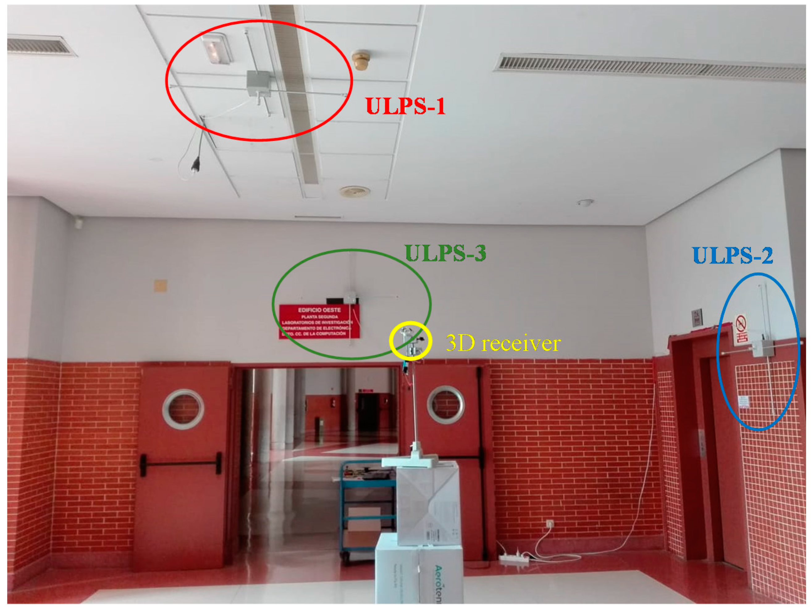
For other types of applications that require 3D positioning, this work proposes hereinafter the use of various ULPS units, which cover the scanned region from diverse points of view in order to obtain an accurate estimation of the receiver’s position in the common coverage volume. Three ULPSs are installed in three perpendicular planes, which define the most common indoor room shapes, pointing to the centre of the volume, whereas other non-central areas are still scanned by at least one of them. Figure 1 depicts the general aspect of this beacon distribution in a normal ordinary-size room. The first ULPS is installed at the ceiling. The other two units are installed on two perpendicular walls [25].
2.1. General Description of LOCATE-US
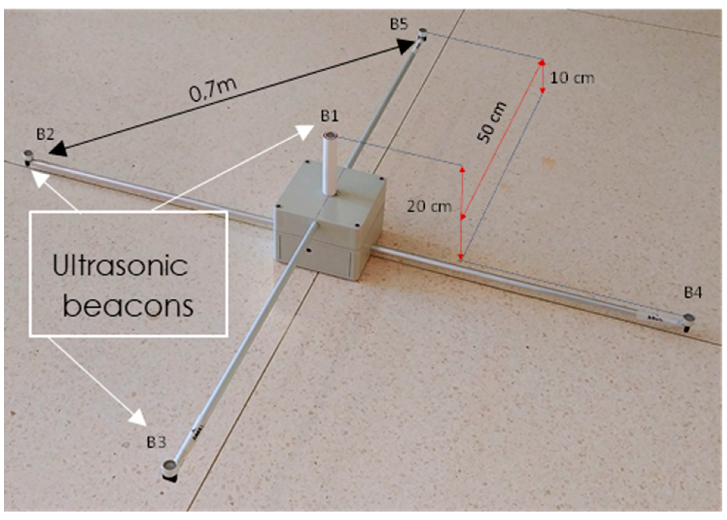
LOCATE-US ULPS is a compact, light, and portable ultrasonic beacon architecture. A single ULPS is formed by five emitter beacons (Bi, where I = 1,2,…5) [26], placed at the centre and at the four corners to form a square with a side of 1/√2 m, as can be observed in Figure 2. The five beacons have been placed in different planes: B2 and B4 are in the base plane, B3 and B5 are moved 10 cm apart, and B1 is moved 20 cm from the base plane [17]. When the ULPS is placed on the ceiling at a height H of 3.5 m emitting top-down, it approximately covers an area of 40 m² and a volume of 53 m3, because the total aperture angle of each emitter is 120°. To avoid audible artefacts, the ULPS operates at roughly 41 kHz [26]. Some ULPSs can be easily deployed to cover wide indoor spaces, where the receiver to be positioned is moving around. Each emitter of the ULPS may use two protocols, code division multiple access (CDMA) and time division multiple access (TDMA), to generate the corresponding emissions, encoded with a different code. These codes present suitable auto-correlation features and low mutual interference with the others. The emitters for a single ULPS can be controlled to configure the ultrasonic transmission in terms of modulation schemes, sampling frequency, and code patterns to be transmitted. Upon reception, a non-limited number of receivers can compute and estimate their own position by measuring TDOAs from the incoming ultrasonic signals inside the coverage volume in an independent and autonomous way. That is why it is not necessary to synchronize the beacons and the receivers [18,27].
It is worth mentioning that, hereinafter, every transducer from the existing ULPSs transmits its own 1023-bit Kasami code so that it can be identified upon reception by matched filtering. These codes are BPSK-modulated at a carrier frequency of 41.67 kHz to adjust the emissions to the available bandwidth.
2.2. General Description of the 3D Ultrasonic Receiver
A 3D ultrasonic receiver assembly has also been designed. It is composed of three receivers, RA, RB, and RC, placed in the three faces of a tetrahedron. This distribution has been adapted to capture ultrasonic transmissions coming from as many directions as possible. All three receivers are wire-synchronized, whereas the general aspect of this 3D ultrasonic receiver is shown in Figure 3a. Three buffers (SD memory) have been added to each receiver to store the acquired signals, where receiver RA is the master and receivers RB and RC are slaves.
The ultrasonic receiver is a small and portable device, consisting of: an omnidirectional MEMS PU0414HR5H-SB microphone [28] with suitable response at 41.67 kHz; an STM32F103 module to filter the received signals with a high-pass filter; and an analog-digital converter at a sampling rate of 100 kHz. Figure 3b presents a single ultrasonic receiver [18]. The omnidirectional MEMS microphone at every face of the 3D assembly receives the ultrasonic signals of similar strength from all the beacons, while minimizing the near-far effect (thanks to the beacons’ distribution). Moreover, all the ultrasonic links have a similar channel model and, consequently, all inter-symbol (ISI) or multiple-access interferences (MAI) are similar. Each receiver is able to capture a buffer with a length of 0.1 s at 100 kHz, so this acquisition window includes at least a complete transmission from the beacons in the ULPSs [18], where a receiver’s position estimate can be obtained in a PC. This feature actually constrains the maximum position update rate of the proposed system to 10 Hz.
2.3. Proposed Positioning Algorithm
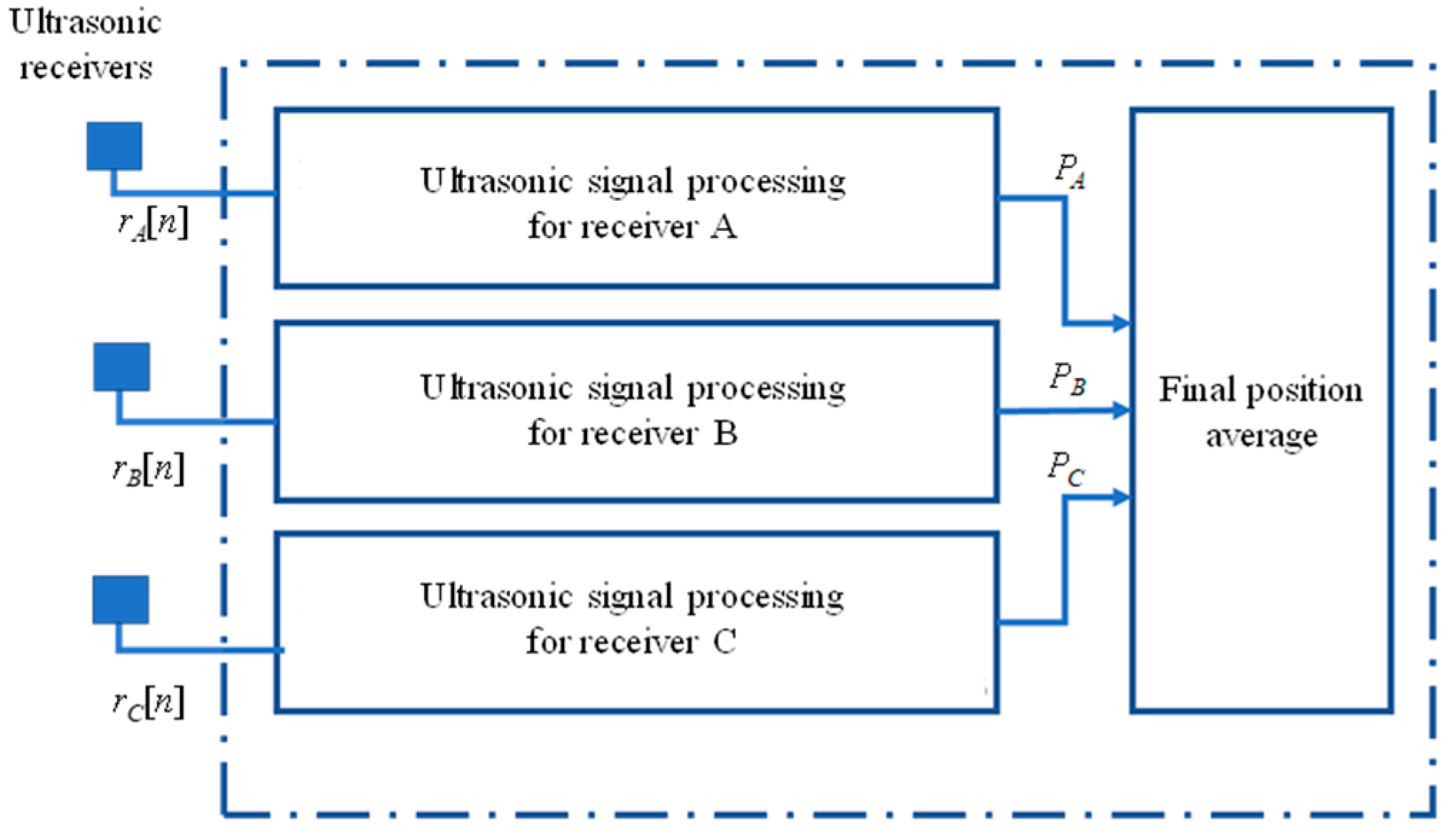
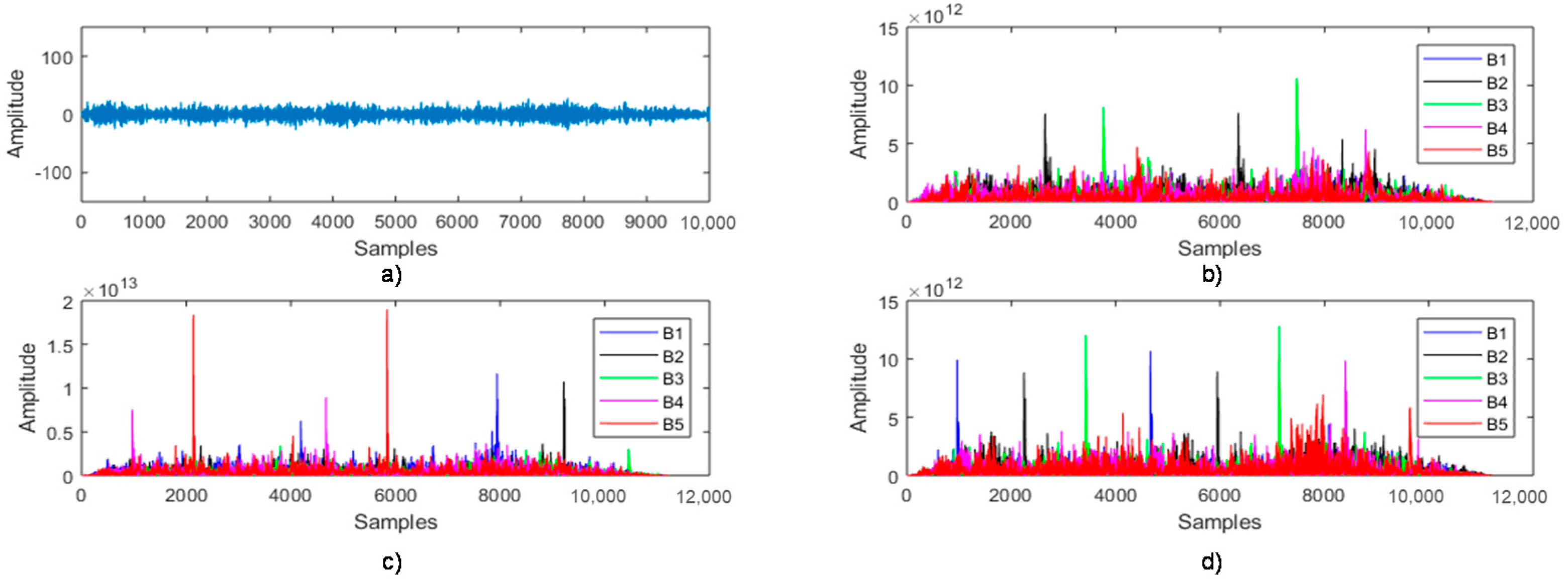
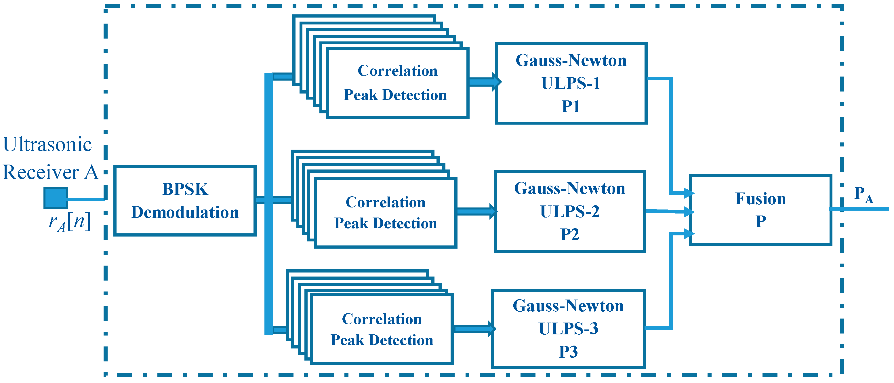
After acquiring the ultrasonic signals from the three available receivers, rA[n], rB[n], and rC[n], a set of BPSK demodulations and correlations with the corresponding emitted 1024-Kasami sequences is implemented. These correlation functions are analysed in order to detect the maximum peak values of the received signals and, consequently, determine the TDOAs between the receiver assembly and the beacons. Afterwards, the TDOAs allow estimation of the receiver’s position by a Hyperbolic Gauss-Newton trilateration technique, because all the ULPSs’ emissions are asynchronous. Taking that into account, as every receiver provides up to five transmissions per ULPS, and the total number of demodulations to compute is three (one per receiver), forty five correlation functions are then implemented. Figure 4 depicts this processing for the 3D receiver assembly [25], whereas Figure 5 shows an example of an incoming acquired signal and the corresponding fifteen correlation functions (for one of the three receivers) with the five emitters from the three available ULPSs.
The position of each receiver is estimated from these time differences using a Gauss–Newton (GN) algorithm, which implies:
- ▪
- Defining an initial position p0 for the receiver (it should be chosen according to the a-priori knowledge of the environment; in our case we consider the centre of the positioning area). In the following steps of the algorithm, this position will be the previously obtained pk−1.
- ▪
- Minimizing the following function f(x, y, z), in the hyperbolic case Equation (1):where are the measured distance differences and are the estimated distance differences computed at the last position of the receiver between the reference beacon B1 and the others Bi (i = 2, …, 5):
- ▪
- Estimating, at each step k, the new position , and repeating the process until (obtained using the GN algorithm [19]) becomes small enough (according to a pre-defined threshold).
Consequently, for any particular test point P, by applying this algorithm at each receiver for each one of the three ULPSs, it is possible to obtain up to three different estimated positions for each receiver RA, RB, and RC, PA (x1, y1, z1), PB (x2, y2, z2), and PC (x3, y3, z3). Note that every ULPS has beacons emitting different codes and, consequently, the receiver is able to discriminate and calculate a position for each ULPS (if a large enough number of time differences is obtained). So, to improve the accuracy of the final position estimate, several fusion algorithms may be used [29]. For the positioning case, the loosely coupled fusion is applied after estimating the receiver’s position for all the emitters, therefore merging these intermediate positions to get the final estimated one. On the other hand, the tightly coupled fusion consists of merging distance differences coming from ULPSs to update the previous positions [30].
3. Proposed Fusion Methods
3.1. Loosely Coupled Approach
The loosely coupled approach, referred to also as the decentralized one, is supposed to integrate the estimated positions, obtained from multiple sensors, to determine the final position. The ultrasonic measurements, coming from the three ULPSs, are used to obtain individual position estimates using the GN algorithm by applying Equations (1) and (2). These position estimates are consequently used as input position measurements in the sensor fusion algorithms (LKF and AKF involved hereinafter), then merged to obtain the final position estimate output of the integrated system with less noise, as well as more accuracy, than the individual estimated positions, as shown in Figure 6. Three identical branches are applied for the three ultrasonic receivers (RA, RB and RC). It is worth noting that the availability of nine position estimates at the input of the fusion module is optimistic, since some of them are often not available.
3.1.1. Linear Kalman Filter Approach
The linear Kalman filter (LKF) is used to merge the estimated positions obtained from the three ULPSs, after applying the GN algorithm. This filter is based on a loop of two steps: prediction and updating. The GN algorithm aims to converge into the correct estimated position after a number of iterations [31]. The state model of the filter is Equation (3):
where Kk is the Kalman filter gain; Q and R the process noise matrix and the measurement noise matrix, respectively; A and H are constant transition matrices; and P is a dynamic matrix. To apply the LKF to fuse the independent estimated positions and obtain the final position, the process and measurement covariance matrices must be fixed experimentally. In our case, the measurement matrix is the covariance of the estimated position related to the specific ULPS. So, the measurement matrix is particular for each position. The process noise Q is fixed experimentally as and computed according to Equation (7), so it is also particular for each position. For the hyperbolic case, it is assumed that the noise is Gaussian for distances and, applied to the distance differences, the noise is correlated, and R and Q are defined as Equations (6) and (7):
where i is the index of the corresponding ULPS, and () are the variances of each position for the three axes x, y, and z, respectively.
3.1.2. Adaptive Kalman Filter Approach
The adaptive Kalman filter (AKF) approach is based on the linear Kalman filter with a dynamic noise matrix Qk to improve the predictions at the instant k [32]. All the initial values are kept as in the LKF case, except the noise matrix that becomes Q0 initially, N is a positive constant, in this case equal to 10, and is the noise error covariance. The final Qk is computed using Equation (8).
where , and
3.2. Tightly Coupled Data Fusion
A tightly coupled approach is supposed to integrate the multiple-sensor raw data (i.e., distance differences) for the position estimation. There are two ways to combine acquired data using specific filters, such as the EKF to deal with the nonlinearities of the positioning equation system. The first way is fusing data in the prediction step of the filter, which employs the values given by the sensors essentially as a control input. So, some sensors are used in the prediction step, whereas the rest of the sensors are used in the update step to correct the prediction [33]. The second way is known as the measurement fusion method [34]; it is the simplest form and consists of fusing data through the observation vector of the filter [35]. The prediction step is then totally based on a mathematical motion model, whereas the update and correction are performed by employing the observations of the sensors [36].
In the implementation of the tightly coupled approach used hereinafter, the second option is involved, due to the direct combination of all the measurements, coming from the ultrasonic sensors, which are used as the observation vector. Thus, this vector consists of the distance differences (obtained from TDOAs) between the ultrasonic transmitters and the mobile receiver. The most relevant advantage is that it does not lose information coming from the pre-processing of the ultrasonic measurements.
The initial position to apply the EKF is estimated using the Gauss-Newton algorithm with the first set of measurements, and for the rest of the steps the positions will be updated feeding the EKF directly with the raw measurements taken. For a single ULPS, the number of required distance differences is at least four. The EKF is also based on a loop of two steps: prediction (13) and updating (14). This algorithm linearizes the state vector and its covariance matrix, applying several observations [37]. Those observations are computed from the US measurements and presented as the distance differences at instant k, () between the mobile receiver (x, y, z) and the beacons i, (xi, yi, zi), and j, (xj, yj, zj). The distance differences Δdij,k are computed from the TDOAs according to Equations (10) and (11):
where c = 340 m/s is the velocity of sound in air; and are the corresponding TDOAs between beacons i and j at instant k.
The state Xk and measurement Zk are given by non-linear functions as in Equation (12):
where is the process noise related to every beacon’s state vector and is the measurement noise at instant k.
The prediction of the state vector and its covariance can be obtained with Equation (13):
where includes information about the movement model (random in a sphere around the previous point position in our case with a radius of 10 cm); Q is the covariance matrix of the process; and Ak is the derivative of with respect to the state vector.
The updated state vector , its covariance , and the Kalman gain are obtained with Equation (14).
where Hk represents the derivative of , defined in (15), with respect to the state vector , giving the matrix shown in Equation (16); Zk is a vector that contains the observations (distance differences) computed using Equation (10); and I is the identity matrix.
The observation estimations are computed by using the a priori state vector and its derivative matrix , according to Equations (15) and (16), respectively.
where is the Euclidean distance between the a priori position estimation and the beacon of the U-LPS considered, with I = {1, 2, 3, …, N}; and are the coordinates of the beacon number 1, used as reference.
The covariance matrix related to the Gaussian observation noise is shown in Equation (17):
where is the standard deviation of the noise in the ultrasonic distance measurements, the experimental value of which has been established at 20 cm for the worst case.
4. Simulated Results
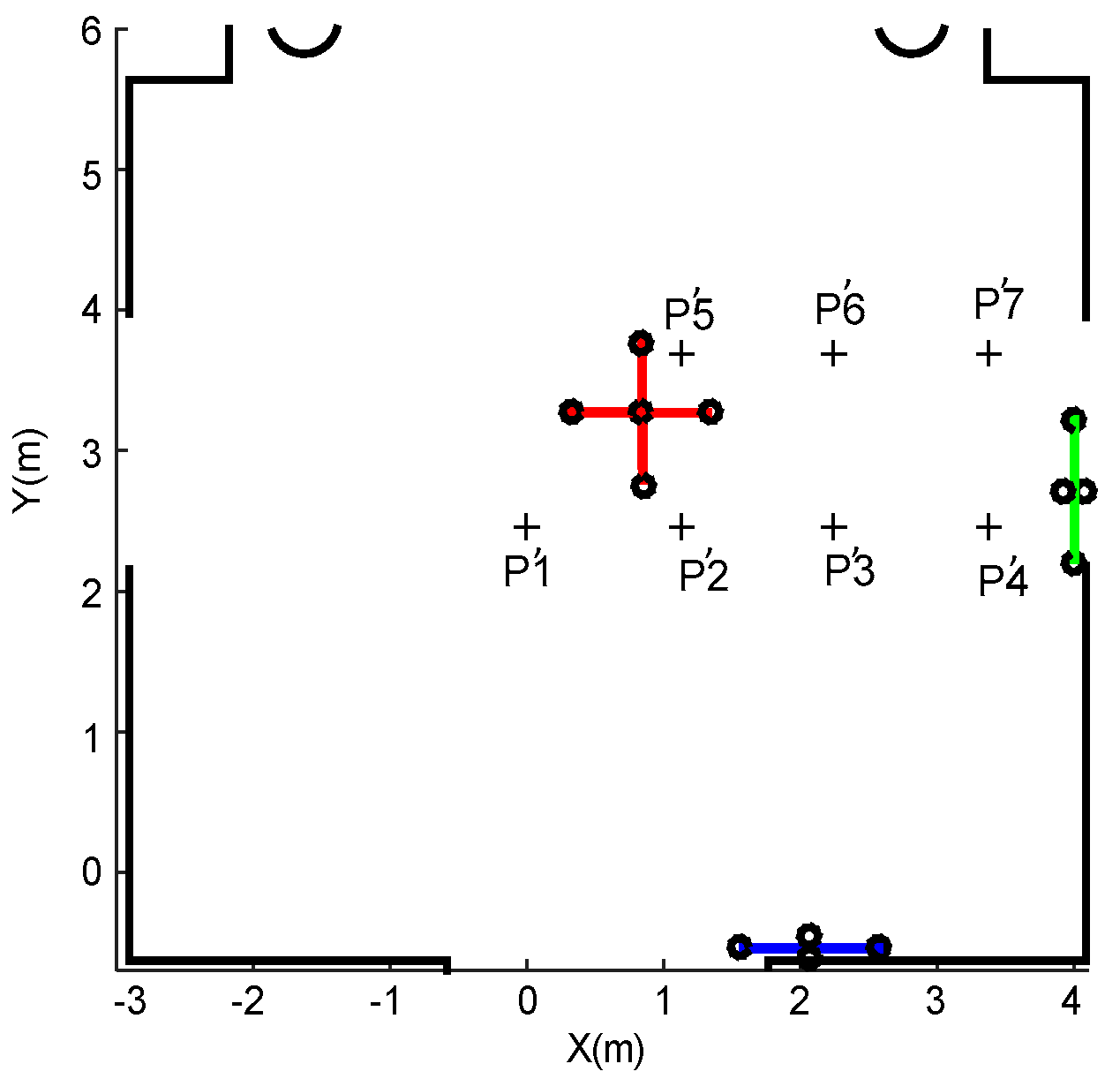
As was mentioned before, the proposed configuration is composed of three ULPSs (ULPS-1, ULPS-2, and ULPS-3) placed at the centres of three perpendicular planes, with the coordinates shown in Table 1. On the other hand, the mobile receiver is placed in a grid of positions (P1–P7), as plotted in Figure 7, defined to analyse the behaviour of the proposal. Twenty realizations were carried out per point in the grid, inserting the aforementioned Gaussian noise in the ultrasonic distance measurement with a null mean and a standard deviation of 20 cm. Every realization was processed independently, according to the scheme in Figure 6, to obtain a final position estimate that was considered for statistical purposes. For this configuration, the positioning algorithm obtained twelve equations, used by the receiver to estimate its own position asynchronously by hyperbolic trilateration with a GN minimization algorithm.
When these ULPSs are working in an independent way, they provide a high dispersion in the position estimation, particularly in the perpendicular directions to each ULPS [19]. For comparison’s sake, this situation was further studied as shown in Table 2, where the mean positioning errors are detailed for the seven considered positions P1–P7 in 90% of cases at two different heights z1 and z2.
Taking into account the previous independent results with significant errors and dispersions in the perpendicular axes to the ULPSs, we propose hereinafter the aforementioned fusion of information at two different levels: a loosely coupled fusion and a tightly coupled one.
4.1. Loosely Coupled Fusion
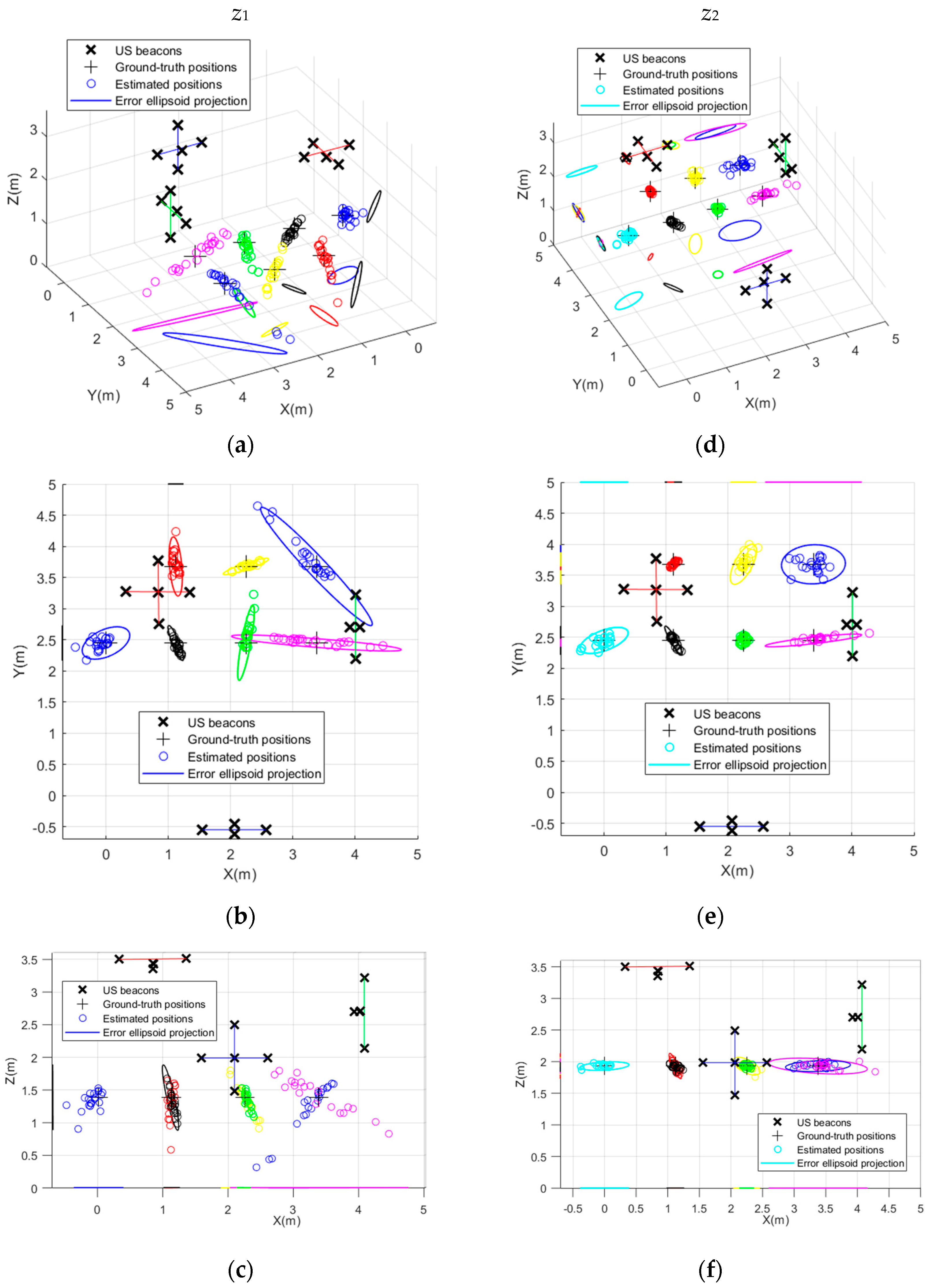
A first alternative consists of applying the LKF to merge the positions estimated from the three ULPSs for the seven positions (P1–P7). This fusion is depicted in Figure 8 at both heights z1 = 1.35 m and z2 = 1.93 m. It is possible to check that the resulting figures are better after fusion, especially at z2, where the estimated positions present variable accuracies. At z1, the most accurate estimated positions are P1, P2, P3, P5, and P6 (cyan, black, green, red, and yellow circles, respectively); also, they present the smallest error ellipsoids for 95% of the estimated positions. On the other hand, the least accurate estimated positions are P4 (pink circles) and P7 (blue circles), as they present the largest error ellipsoids for 95% of the estimated positions. Similar conclusions can be derived for z2, with errors even lower. This effect is related to the distance between those positions and ULPS-2. Table 3 presents those results by providing the mean error and the standard deviation per axis for the seven considered points (P1–P7).
To compare the accuracy provided by the LKF with that from the independent ULPSs in Table 2, Table 4 provides the errors for 90% of estimated positions. It is worth noting that the positioning errors are now in the range of centimetres or decimetres. At height z1, the error for positions P1, P2, P3, P5, and P6 is below 0.34 m, whereas it is below 0.7 m for P4 and P7. In the case of z2, the errors for all positions P1–P7 are below 0.29 m for 90% of cases.
A second approach considered here is to apply an AKF. Figure 9 presents the fusion results at z1 and z2. Similar conclusions can be derived: as before, the best estimated positions are P1, P2, P3, P5, and P6 (cyan, black, green, red, and yellow circles, respectively), and they also present the smallest error ellipsoids for 95% of estimated positions, whereas the worst ones are P4 (pink circles) and P7 (blue circles). The mean error and the standard deviation per axis are provided in Table 5, whereas Table 6 describes the positioning error for 90% of cases. The positioning error of the estimates reached by simulation is again in the range of centimetres or decimetres. Although results from the LKF are similar to those from the AKF, the second approach presents better accuracy due to the update of the values in the noise matrix of the filter. Globally, the mean error for 90% of the estimated positions is below 0.27 m at z1 and 0.101 m at z2.
4.2. Tightly Coupled Fusion
In the tightly coupled approach, it is proposed to use an EKF to fuse the raw distance measurements from the three existing ULPSs, in order to estimate the final receiver’s position. Note that, in this approach, the fusion method does not deal with the intermediate positions obtained for each ULPS independently, but merges the distance differences determined by every ULPS into a single EKF to obtain the final position.
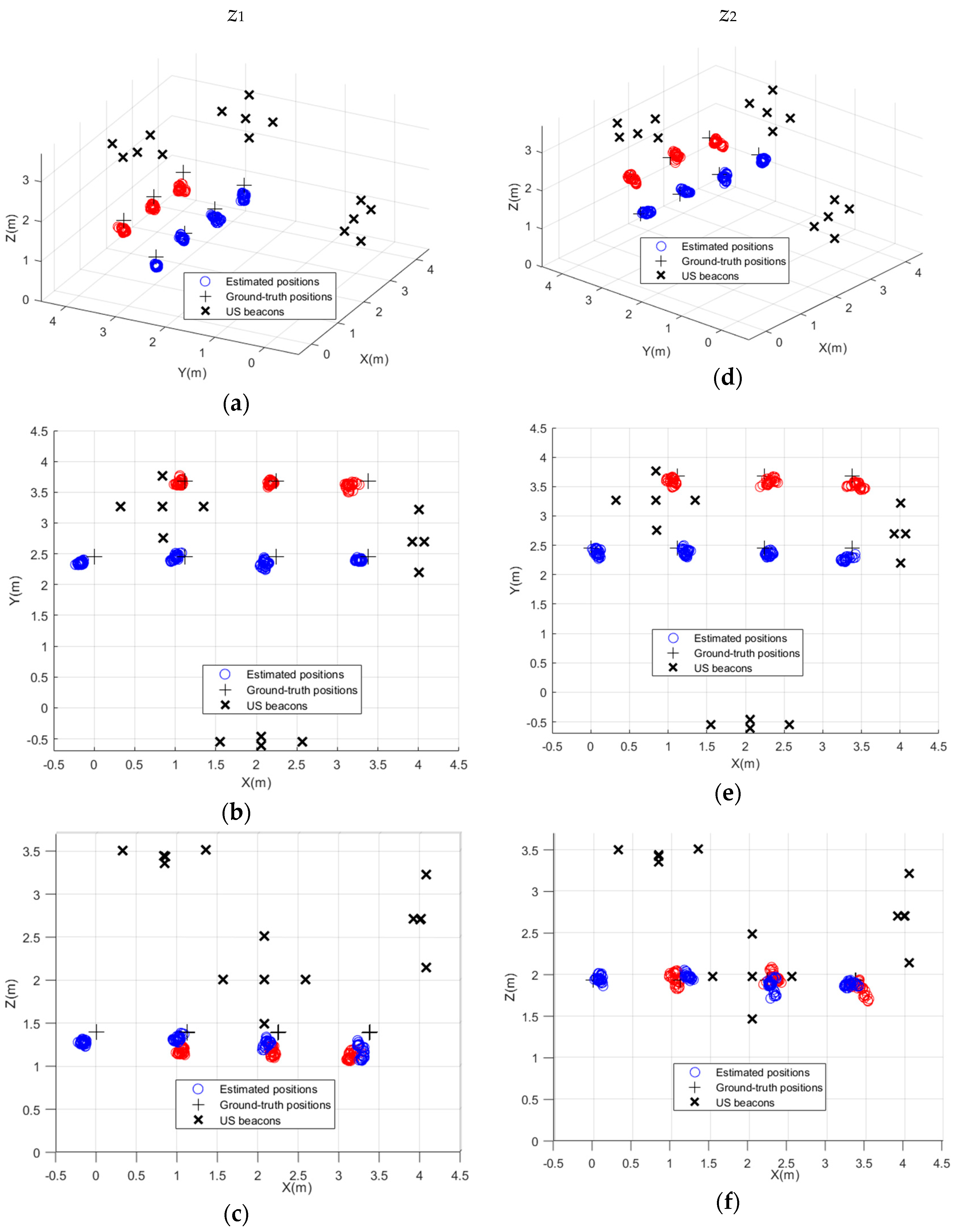
Simulations have been carried out for the seven positions P1–P7 at z1 and z2, with a typical deviation . As before, Figure 10 plots the clouds of positions, which are more concentrated around the ground-truth points, with lower dispersions. The mean errors and the standard deviations are listed in Table 7. Finally, the errors for 90% of the cases for the seven studied points P1–P7 are between 0.107 and 0.3 m at z1, and between 0.105 and 0.2 m at z2, as can be derived from Figure 11.
Summing up, the first approach proposed here is based on the fusion of the obtained positions with the so-called loosely coupled fusion method, where two different algorithms have been applied: the LKF and AKF. On the other hand, from the point of view of the tightly coupled fusion, an EKF has been proposed for the raw measurements from the three ULPSs. Table 8 summarizes the errors for 90% of the estimated positions. It is possible to observe that the tightly coupled method is more accurate than the loosely coupled ones.
5. Experimental Results
Some experimental results are presented now, according to the previously studied fusion algorithms. These tests were developed in a hall of the School of Engineering at the University of Alcala. As shown in Figure 1, it is an extended hall located on the second floor of the building, with a volume of 7 × 8 × 3.5 m3. Table 1 already showed the coordinates of the central beacons B1 for every ULPS; note that ULPS-2 and ULPS-3 had different heights and were not placed at the centres of the wall in the hall, due to its complex architecture.
The beacons from the three ULPSs were encoded with fifteen different 1023-bit Kasami sequences, whereas a multiple ultrasonic receiver prototype was placed at the seven measurement points (P1–P7) with the same heights z1 = 1.35 m and z2 = 1.93 m, in accordance with the previous simulations. Firstly, one hundred measurements were acquired and stored at each position for the three ULPSs. Those measurements were used to compute the variances of each position offline, then stored and used later in the online positioning system, when the variances were needed in the loosely coupled fusion methods. Secondly, thirty measurements were obtained at each point P1–P7 for the online study. These experimental results are provided next, in the same order as they were analysed in Section 4 for simulations.
Table 9 shows the positioning errors for 90% of the cases, when the three ULPSs operated independently, with errors varying in the decimetre and meter ranges.
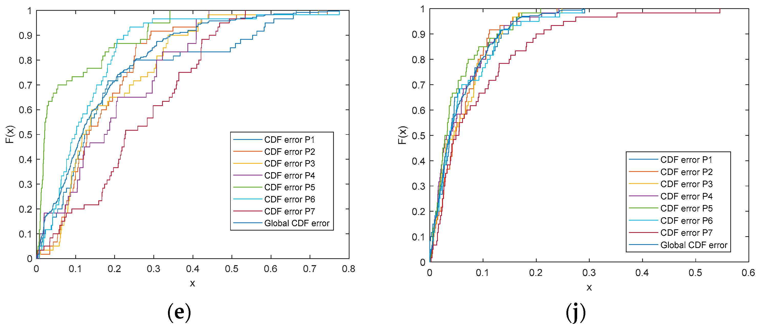
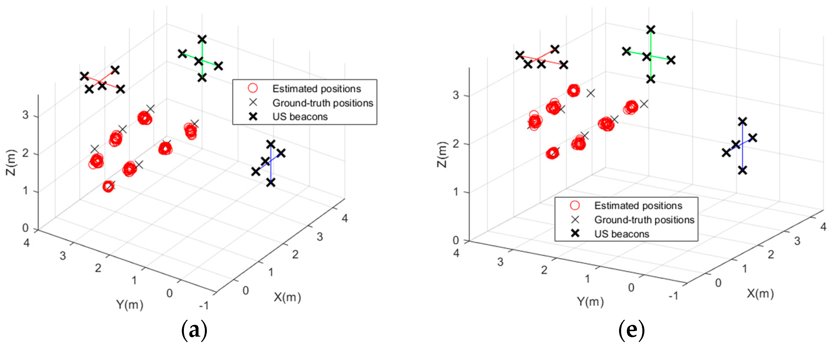
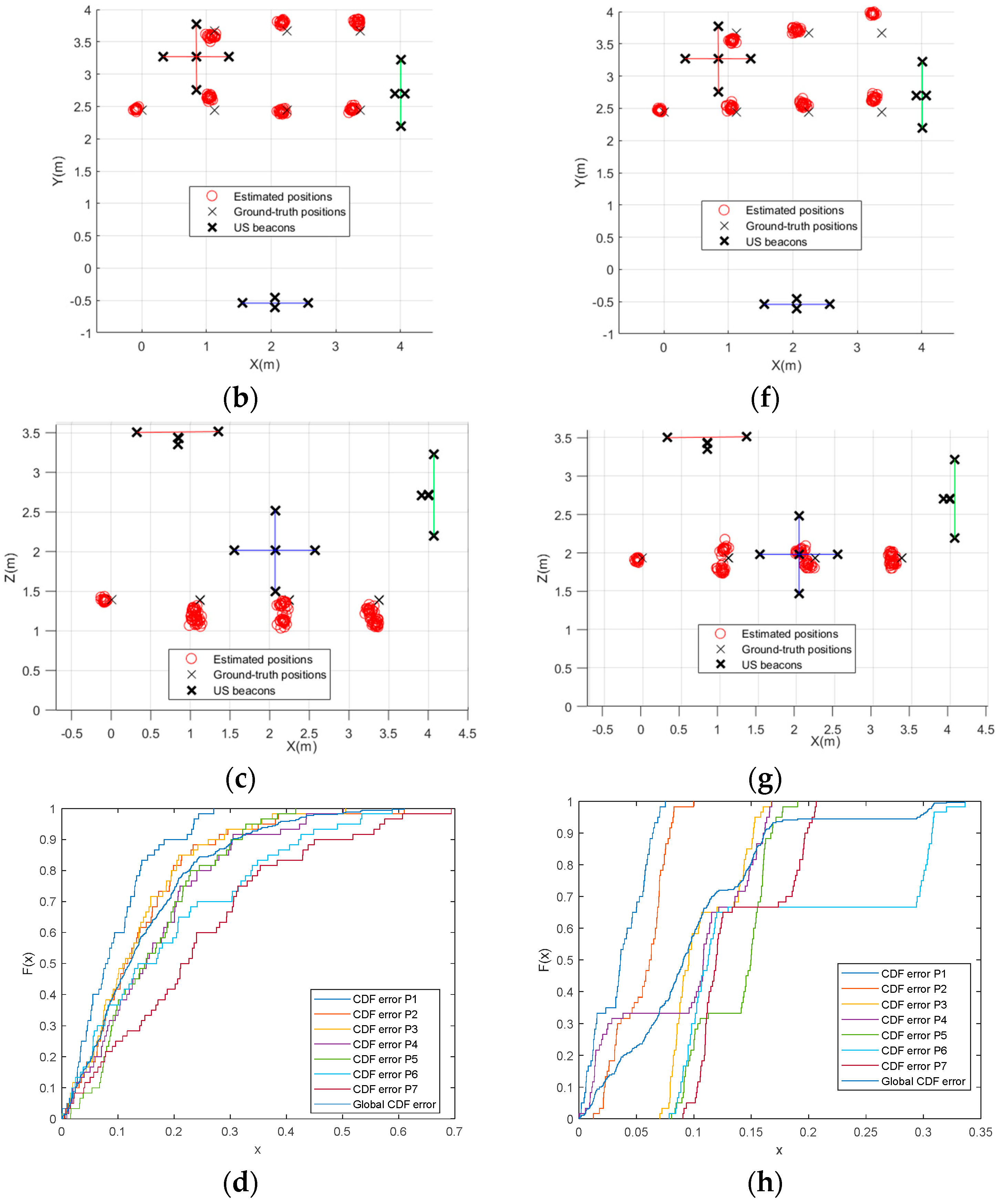
With regard to the LKF in the loosely coupled fusion, Figure 12 plots the estimated positions after fusion, with their different plane projections at both heights. The LKF merged up to nine position estimates, as there were three ULPSs and three receivers in the experimental prototype. Additionally, a CDF error is plotted for both cases in Figure 12e,j, where the average error for all the points is 0.72 m at z1 and 0.34 m at z2. Table 10 shows the mean error and standard deviation for P1–P7. The height z2 was more accurate for the three axes.
Concerning the AKF, Figure 13 shows the experimental results for the set of points (P1–P7) at both heights z1 and z2, in the same format as before. In this case, the mean CDF error was 0.346 m at z1, whereas it was 0.162 m at z2. Furthermore, Table 11 shows the mean error and standard deviation at both heights. The height z1 presented a large error in the z-axis, higher than 0.14 m for all the grid, whereas at z2 this error decreased to less than 0.03 m. The positions at z2 were always more accurate for the three axes.
Finally, some results from the EKF applied as a tightly coupled method are presented in Figure 14 with variance in the measurements of distances fixed at σw = 0.2 m. As was confirmed in simulations previously, the clouds of the seven positions were more concentrated around the ground-truth points, with low dispersions as well. The mean errors and standard deviations are listed in Table 12. It is worth mentioning that all the axis errors decreased for both heights, especially for z2, to less than 0.17 m at z1 and less than 0.13 m at z2. The CDF errors for 90% of the cases for the seven studied points were between 0.18 and 0.45 m at z1, and between 0.06 and 0.3 m at z2, as plotted in Figure 14d,h.
In summary, the experimental results in Table 13 corroborated the positioning errors previous simulations listed in Table 8. It is possible to observe that the tightly coupled method applying an EKF presents more accurate estimated positions, where the mean error for the grid of positions is less than 0.3 m at z1 and about 0.15 m at z2. In addition, this method is capable of providing a valid estimate in all the realizations, thus implying high availability. A key comparison can be made with the results in Table 9, for the scenario when the ULPS are working independently. It is possible to observe that errors in Table 10, Table 11 and Table 12 are considerably reduced by merging the measurements from the three ULPS. The height z1 leads to higher errors, where each point P1–P7 is particularly complicated for a different independent ULPS, according to their position. On the other hand, the approaches based on measurement fusion allow these restrictions to be compensated, thus yielding more than four times smaller errors.
With regard to previous works dealing with the design of ultrasonic positioning systems, a proposal based on a single ULPS was described in [18] for 2D positioning, with errors below 20 cm in 90% of the cases for a grid of points on the ground with a size of 4 × 4 m2. After the fusion process proposed here, errors were also below 20 cm for 90% of the cases involving the EFK approach (tightly coupled), but considering a 3D positioning, which was already a significant improvement. In [27], the ultrasonic measurements were merged with those coming from inertial measurement units (IMU), as well as with graphs defined and matched by maps from the navigation environments. In this case, the ultrasonic system was only used to correct the accumulative errors from the inertial sensors, applied to the guidance and monitoring of people in indoor environments. Another 3D positioning system based on ultrasound was presented in [3], where mean errors below 1 cm were reported. Nevertheless, it is worth noting that that proposal applied a sequential polling for every beacon, as well as a different ultrasonic signal processing approach with a higher computational load than the one described here. Finally, in [38], average errors in 3D ultrasonic positioning around 9.5 cm were reported, which was in the same range as the ones presented in Table 7 and Table 12 for the EKF approach.
6. Conclusions
This work presented a 3D ultrasonic positioning system, as well as developed positioning and fusion algorithms. This structure is composed of three ULPSs installed in three perpendicular walls with the aim of covering almost the whole space of a common room shape. Moreover, a 3D ultrasonic receiver prototype is used to acquire signals coming from different directions. Then, several fusion algorithms were tested based on two different approaches: the loosely coupled and tightly coupled one. Taking into account that two heights were studied for all considered algorithms, the height z2 had more accurate positions due to its specific location with respect to the three ULPSs, especially for ULPS-2 and ULPS-3 (the same height). Additionally, the tightly coupled approach presented lower errors in general terms at both heights z1 and z2. However, the AKF fusion also provided good accuracy for the loosely coupled approach at z2. Generally, the positioning error was in the decimetre range for the different studied configurations, which makes the proposal suitable for numerous indoor positioning applications, such as logistics in warehouses, tourist guidance in museums and historical buildings, or accurate positioning in independent living settings for the elderly.
A last aspect to consider is the scalability of the proposal. The aforementioned LOCATE-US system can be extended to larger environments by suitably distributing the ULPSs to cover the desired area, or by increasing the number of installed ULPSs. Furthermore, the ultrasonic beacons in every ULPS can be separated to better fit the requirements of a given environment (note that in this case an infrared link is used to synchronize simultaneous emissions from all the beacons).
Author Contributions
Conceptualization, J.U., K.M. and Á.H.; methodology, J.U. and J.M.V.; software, K.M.; validation and formal analysis, J.U., M.M. and K.M.; investigation, J.U., K.M., Á.H. and T.A.; writing—original draft preparation, K.M.; writing—review and editing, Á.H. and J.M.V.; supervision, J.U.; funding acquisition, J.U. and J.M.V. All authors have read and agreed to the published version of the manuscript.
Funding
This work has been supported by the Spanish Ministry of Science, Innovation and Universities (MICROCEBUS project, ref. RTI2018-095168-BC51, and POM project, ref. PID2019-105470RA-C33), the Community of Madrid (PUILPOS project, ref. CM/JIN/2019-038, and CODEUS project, ref. CM/JIN/2019-043).
Institutional Review Board Statement
Not applicable.
Informed Consent Statement
Not applicable.
Data Availability Statement
Not applicable.
Conflicts of Interest
Not applicable.
References
- Mendoza-Silva, G.M.; Torres-Sospedra, J.; Huerta, J. A meta-review of indoor positioning systems. Sensors 2019, 19, 4507. [Google Scholar] [CrossRef] [PubMed] [Green Version]
- Mautz, R. Indoor Positioning Technologies. Ph.D. Thesis, ETH Zurich, Zurich, Switzerland, 2012. [Google Scholar]
- De Angelis, A.; Moschitta, A.; Carbone, P.; Calderini, M.; Neri, S.; Borgna, R.; Peppucci, M. Design and characterization of a portable ultrasonic indoor 3-D positioning system. IEEE Trans. Instrum. Meas. 2015, 64, 2616–2625. [Google Scholar] [CrossRef]
- Yucel, H.; Edizkan, R.; Ozkir, T.; Yazici, A. Development of indoor positioning system with ultrasonic and infrared signals. In Proceedings of the 2012 IEEE International Symposium on Innovations in Intelligent Systems and Applications, Trabzon, Turkey, 2 July 2012; pp. 1–4. [Google Scholar]
- Sertatil, C.; Altinkaya, M.A.; Raoof, K. A novel acoustic indoor localization system employing CDMA. Digit. Signal. Process. 2012, 22, 506–517. [Google Scholar] [CrossRef] [Green Version]
- Lin, Q.; An, Z.; Yang, L. Rebooting ultrasonic positioning systems for ultrasound-incapable smart devices. In Proceedings of the 25th Annual International Conference on Mobile Computing and Networking, Los Cabos, Mexico, 25 October 2019; pp. 1–16. [Google Scholar]
- Kapoor, R.; Ramasamy, S.; Gardi, A.; Bieber, C.; Silverberg, L.; Sabatini, R. A novel 3D multilateration sensor using distributed ultrasonic beacons for indoor navigation. Sensors 2016, 16, 1637. [Google Scholar] [CrossRef] [Green Version]
- Kapoor, R.; Gardi, A.; Sabatini, R. Acoustic positioning and navigation system for gnss denied/challenged environments. In Proceedings of the 2020 IEEE/ION Position, Location and Navigation Symposium (PLANS), Portland, OR, USA, 20 April 2020; pp. 1280–1285. [Google Scholar]
- Saad, M.M.; Bleakley, C.J.; Ballal, T.; Dobson, S. High-accuracy reference-free ultrasonic location estimation. IEEE Trans. Instrum. Meas. 2012, 61, 1561–1570. [Google Scholar] [CrossRef]
- Prieto, J.C.; Jiménez, A.R.; Guevara, J.; Ealo, J.L.; Seco, F.; Roa, J.O.; Ramos, F. Performance evaluation of 3D-LOCUS advanced acoustic LPS. IEEE Trans. Instrum. Meas. 2009, 58, 2385–2395. [Google Scholar] [CrossRef]
- Lopes, S.I.; Vieira, J.M.N.; Albuquerque, D. High accuracy 3D indoor positioning using broadband ultrasonic signals. In Proceedings of the 2012 IEEE 11th International Conference on Trust, Security and Privacy in Computing and Communications, Liverpool, UK, 25 June 2012; pp. 2008–2014. [Google Scholar]
- Suzuki, A.; Iyota, T.; Choi, Y.; Kubota, Y.; Watanabe, K.; Yamane, A. Measurement accuracy on indoor positioning system using spread spectrum ultrasonic waves. In Proceedings of the 2009 4th IEEE International Conference on Autonomous Robots and Agents, Wellington, New Zealand, 10 February 2009; pp. 294–297. [Google Scholar]
- Schweinzer, H.; Syafrudin, M. LOSNUS: An ultrasonic system enabling high accuracy and secure TDoA locating of numerous devices. In Proceedings of the 2010 International Conference on Indoor Positioning and Indoor Navigation, Zurich, Switzerland, 15 September 2010; pp. 1–8. [Google Scholar]
- Sato, T.; Nakamura, S.; Terabayashi, K.; Sugimoto, M.; Hashizume, H. Design and implementation of a robust and real-time ultrasonic motion-capture system. In Proceedings of the 2011 International Conference on Indoor Positioning and Indoor Navigation, Guimarães, Portugal, 21 September 2011; pp. 1–6. [Google Scholar]
- Nakamura, S.; Sato, T.; Sugimoto, M.; Hashizume, H. An accurate technique for simultaneous measurement of 3D position and velocity of a moving object using a single ultrasonic receiver unit. In Proceedings of the 2010 International Conference on Indoor Positioning and Indoor Navigation, Zurich, Switzerland, 15 September 2010; pp. 1–7. [Google Scholar]
- Khyam, M.O.; Alam, M.J.; Lambert, A.J.; Benson, C.R.; Pickering, M.R. High precision ultrasonic positioning using phase correlation. In Proceedings of the 2012 6th International Conference on Signal Processing and Communication Systems, Gold Coast, Australia, 12–14 December 2012; pp. 1–6. [Google Scholar]
- Hernández, A.; García, E.; Gualda, D.; Villadangos, J.M.; Nombela, F.; Ureña, J. FPGA-based architecture for managing ultrasonic beacons in a local positioning system. IEEE Trans. Instrum. Meas. 2017, 66, 1954–1964. [Google Scholar] [CrossRef]
- Ureña, J.; Hernández, A.; García, J.J.; Villadangos, J.M.; Pérez, M.C.; Gualda, D.; Álvarez, F. Acoustic local positioning with encoded emission beacons. Proc. IEEE 2018, 106, 1042–1062. [Google Scholar] [CrossRef]
- Mannay, K.; Ureña, J.; Hernández, A.; Machhout, M.; Aguili, T. Characterization of an ultrasonic local positioning system for 3D measurements. Sensors 2020, 20, 1–23. [Google Scholar]
- Hall, D.; Llinas, J. Multisensor Data Fusion; CRC Press: Boca Raton, FL, USA, 2001. [Google Scholar]
- Varshney, P.K. Multisensor data fusion. Electron. Commun. Eng. J. 1997, 9, 245–253. [Google Scholar] [CrossRef]
- Castanedo, F. A review of data fusion techniques. Sci. World J. 2013, 2013, 1–20. [Google Scholar] [CrossRef] [PubMed]
- Haug, A.J. Bayesian Estimation and Tracking: A Practical Guide; John Wiley & Sons: Hoboken, NJ, USA, 2012. [Google Scholar]
- Gualda, D.; Ureña, J.; García, J.C.; García, E.; Alcalá, J. Simultaneous calibration and navigation (SCAN) of multiple ultrasonic local positioning systems. Inf. Fusion 2019, 45, 53–65. [Google Scholar] [CrossRef]
- Mannay, K.; Ureña, J.; Hernández, A.; Machhout, M.; Aguili, T. Analysis of performance of ultrasonic local positioning systems for 3D spaces. In Proceedings of the 2017 International Conference on Indoor Positioning and Indoor Navigation (IPIN 2017), Sapporo, Japan, 18 September 2017; Volume 1, pp. 1–5. [Google Scholar]
- Pro-Wave Electronics Corporation. Air Ultrasonic Ceramic Transducers 328ST/R160; Product Specification: New Taipei City, Taiwan, 2014. [Google Scholar]
- Gualda, D.; Pérez-Rubio, M.C.; Ureña, J.; Pérez-Bachiller, S.; Villadangos, J.M.; Hernández, A.; García, J.J.; Jiménez, A. LOCATE-US: Indoor positioning for mobile devices using encoded ultrasonic signals, inertial sensors and graph-matching. Sensors 2021, 21, 1950. [Google Scholar] [CrossRef] [PubMed]
- Knowles Acoustics LLC. Amplified “Ultra-Mini” SiSonicTM Microphone Specification with MaxRF Protection, SPU0414HR5H-SB; Product Specification: Itasca, IL, USA, 2012. [Google Scholar]
- Bhatia, D.; Paul, S. Sensor fusion and control techniques for biorehabilitation. In Bioelectronics and Medical Devices; Woodhead Publishing: Sawston, UK, 2019; pp. 615–634. [Google Scholar]
- Nurmi, J.; Lohan, E.-S.; Wymeersch, H.; Seco-Granados, G.; Nykänen, O. Multi-Technology Positioning; Springer: Berlin/Heidelberg, Germany, 2017. [Google Scholar]
- Kalman, R.E.; Bucy, R.S. New results in linear filtering and prediction theory. J. Basic Eng. 1961, 83, 95–108. [Google Scholar] [CrossRef]
- Yang, Y.; Gao, W. An optimal adaptive Kalman filter. J. Geod. 2006, 80, 177–183. [Google Scholar] [CrossRef]
- Rhudy, M.; Gross, J.; Gu, Y.; Napolitano, M. Fusion of GPS and redundant IMU data for attitude estimation. In Proceedings of the AIAA Guidance, Navigation, and Control Conference, Minneapolis, MN, USA, 13 August 2012; pp. 5030–5043. [Google Scholar]
- Gan, Q.; Harris, C.J. Comparison of two measurement fusion methods for Kalman-filter-based multisensor data fusion. IEEE Trans. Aerosp. Electron. Syst. 2001, 37, 273–279. [Google Scholar] [CrossRef] [Green Version]
- Benini, A.; Mancini, A.; Marinelli, A.; Longhi, S. A biased extended kalman filter for indoor localization of a mobile agent using low-cost imu and uwb wireless sensor network. IFAC Proc. Vol. 2012, 45, 735–740. [Google Scholar] [CrossRef] [Green Version]
- Miraglia, G.; Maleki, K.N.; Hook, L.R. Comparison of two sensor data fusion methods in a tightly coupled UWB/IMU 3-D localization system. In Proceedings of the 2017 International Conference on Engineering, Technology and Innovation (ICE/ITMC), Madeira, Portugal, 27 June 2017; pp. 611–618. [Google Scholar]
- Cox, H. On the estimation of state variables and parameters for noisy dynamic systems. IEEE Trans. Autom. Control. 1964, 9, 5–12. [Google Scholar] [CrossRef]
- Kapoor, R.; Gardi, A.; Sabatini, R. Network optimisation and performance analysis of a multistatic acoustic navigation sensor. Sensors 2020, 20, 5718. [Google Scholar] [CrossRef] [PubMed]
Figure 1.
General view of the 3D scenario considered with three ULPS units installed on three perpendicular planes of the environment and a mobile receiver.
Figure 1.
General view of the 3D scenario considered with three ULPS units installed on three perpendicular planes of the environment and a mobile receiver.

Figure 2.
General view of LOCATE-US ULPS unit.

Figure 3.
General aspect of the 3D receiver assembly: (a) the receiver assembly based on three single receivers; (b) a view of a single receiver.
Figure 3.
General aspect of the 3D receiver assembly: (a) the receiver assembly based on three single receivers; (b) a view of a single receiver.

Figure 4.
General block diagram of the processing proposed for the multiple receiver prototype.

Figure 5.
Example of the incoming acquired rA[n] in a single receiver (a), as well as the correlation functions for the three available ULPSs (b–d).
Figure 5.
Example of the incoming acquired rA[n] in a single receiver (a), as well as the correlation functions for the three available ULPSs (b–d).

Figure 6.
Block diagram of a loosely coupled fusion of the three positions estimated by the receiver RA.
Figure 6.
Block diagram of a loosely coupled fusion of the three positions estimated by the receiver RA.

Figure 7.
Workspace configuration and grid of positions considered to evaluate the positioning performance. ULPS-1 is plotted in red, ULPS-2 in blue, and ULPS-3 in green.
Figure 7.
Workspace configuration and grid of positions considered to evaluate the positioning performance. ULPS-1 is plotted in red, ULPS-2 in blue, and ULPS-3 in green.

Figure 8.
(a–f) Estimated positions after the LKF fusion for the points P1–P7, including the projections of their corresponding error ellipsoids with a certainty of 95% in the XY and XZ planes, at z1 = 1.35 m (left) and z2 = 1.93 m (right): successively, 3D representation of clouds of points; Y–X projections; and Z–X projections.

Figure 9.
(a–f) Estimated positions after AKF fusion for the points P1–P7, including the projections of their corresponding error ellipsoids with a certainty of 95% in the XY and XZ planes, at z1 = 1.35 m (left) and z2 = 1.93 m (right): successively, 3D representation of clouds of points; Y–X projections; and Z–X projections.

Figure 10.
(a–f) Clouds of estimated positions with an EKF and three ULPSs for σw = 0.2 m, at z1 = 1.35 m (left) and z2 = 1.93 m (right): successively, 3D representation of clouds of points; Y–X projections; and Z–X projections.
Figure 10.
(a–f) Clouds of estimated positions with an EKF and three ULPSs for σw = 0.2 m, at z1 = 1.35 m (left) and z2 = 1.93 m (right): successively, 3D representation of clouds of points; Y–X projections; and Z–X projections.

Figure 11.
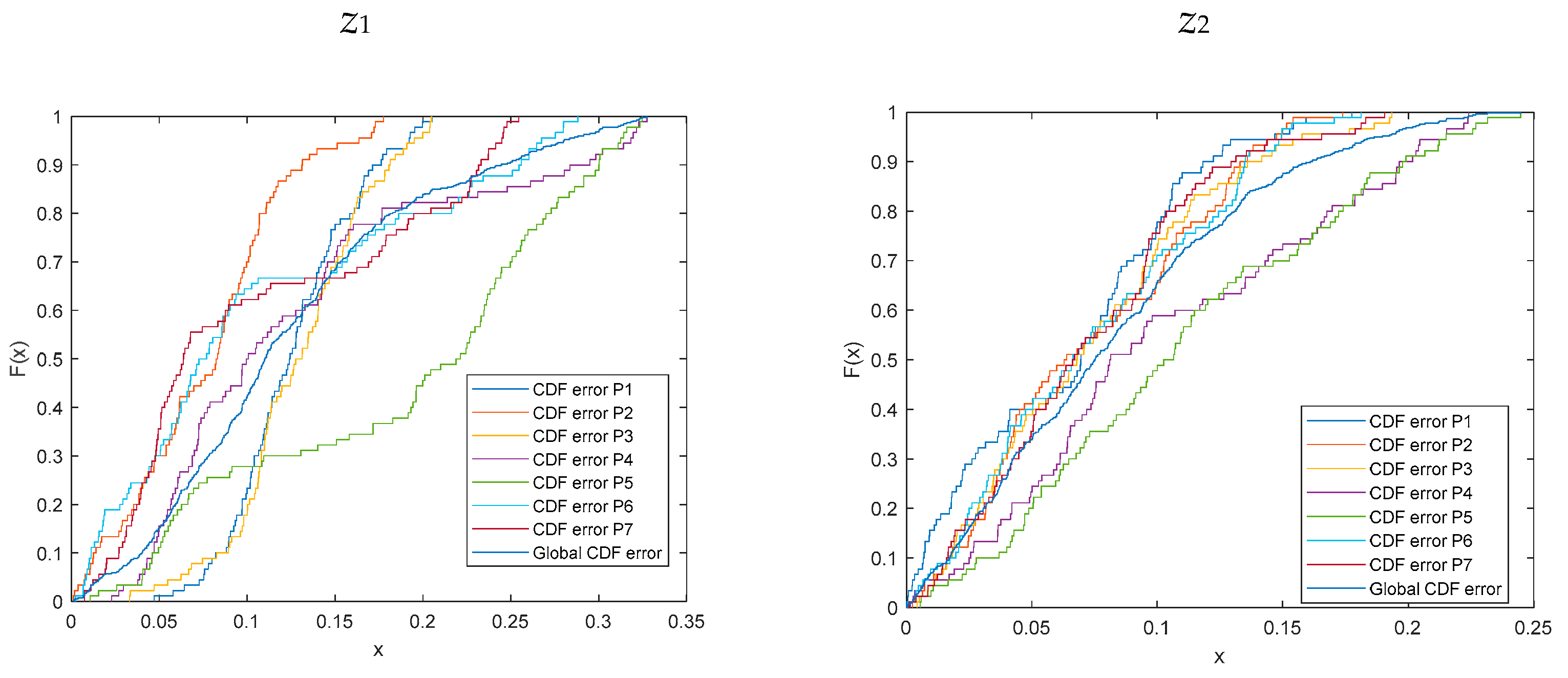
Positioning errors (CDF), for an EKF and three ULPS (σw = 0.2 m), for the three coordinates, x, y and z, for the grid of positions (P1–P7), at z1 = 1.35 m (left) and z2 = 1.93 m (right).
Figure 11.
Positioning errors (CDF), for an EKF and three ULPS (σw = 0.2 m), for the three coordinates, x, y and z, for the grid of positions (P1–P7), at z1 = 1.35 m (left) and z2 = 1.93 m (right).

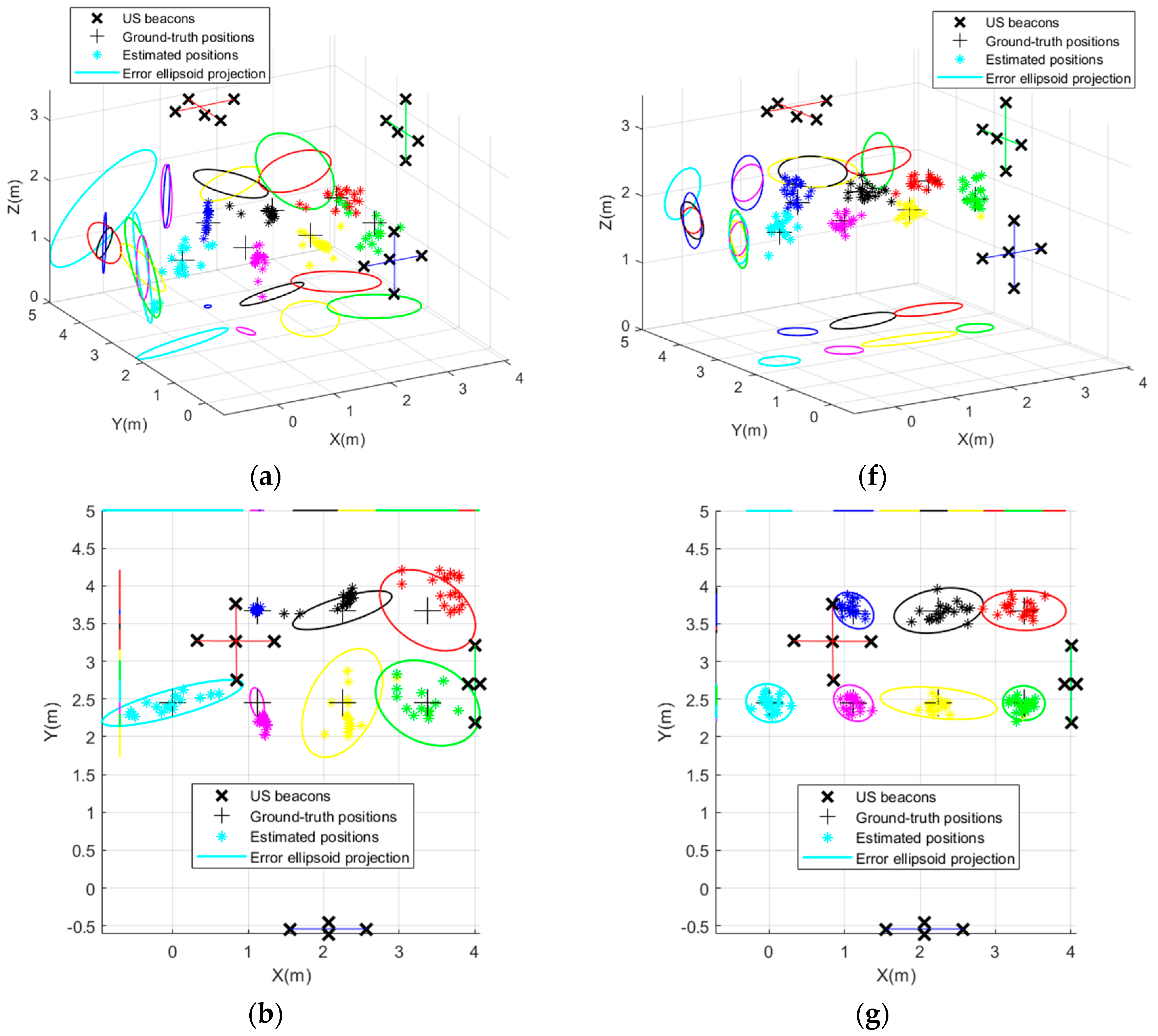
Figure 12.
Experimental results for the tested points P1–P7 for both heights, z1 = 1.35 m on the left (a–e) and z2 = 1.93 m on the right (f–j): successively, 3D representation of clouds of points; Y–X projections; Z–X projections; Z–Y projections; and experimental CDFs for each point after LKF fusion.


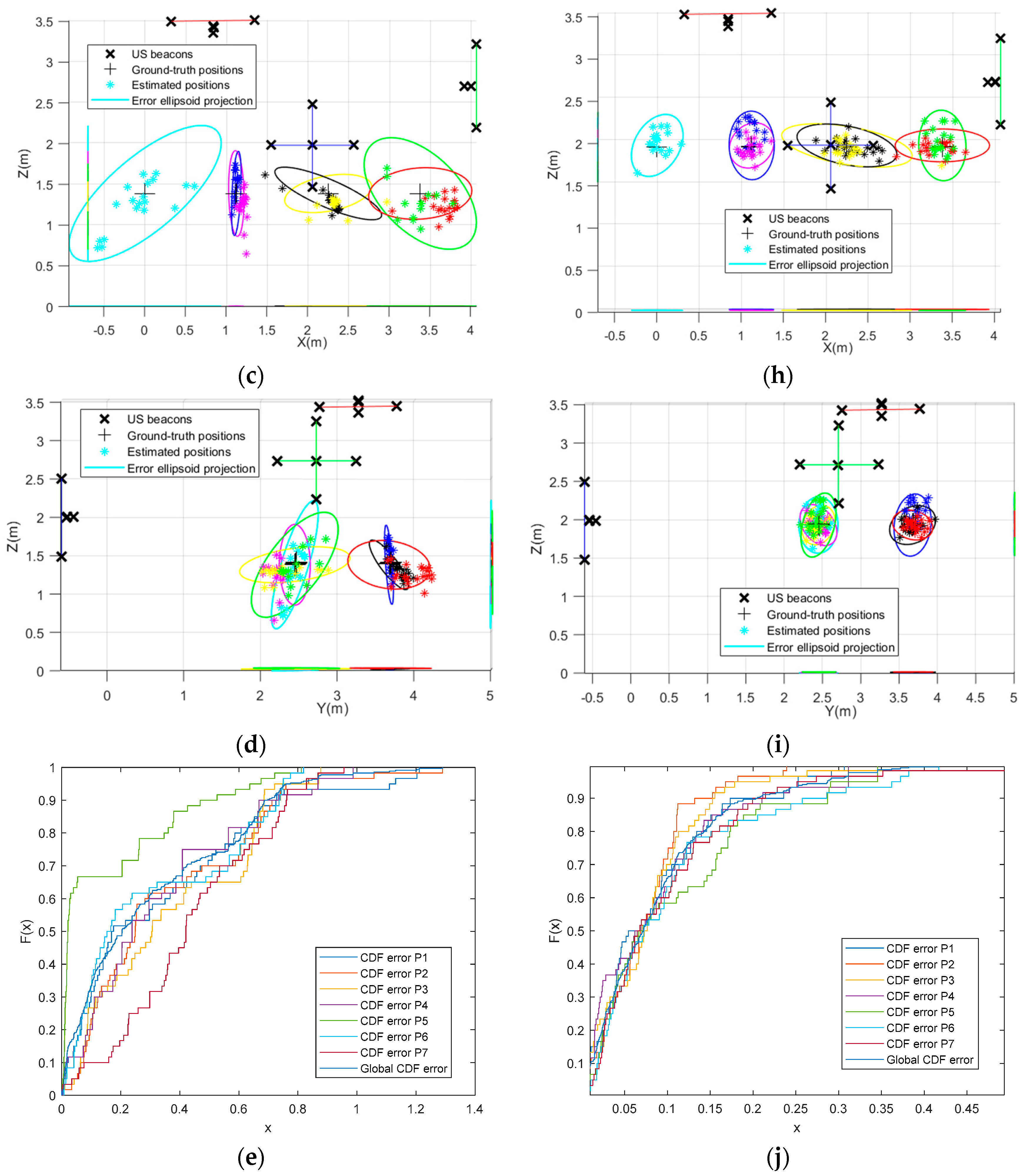
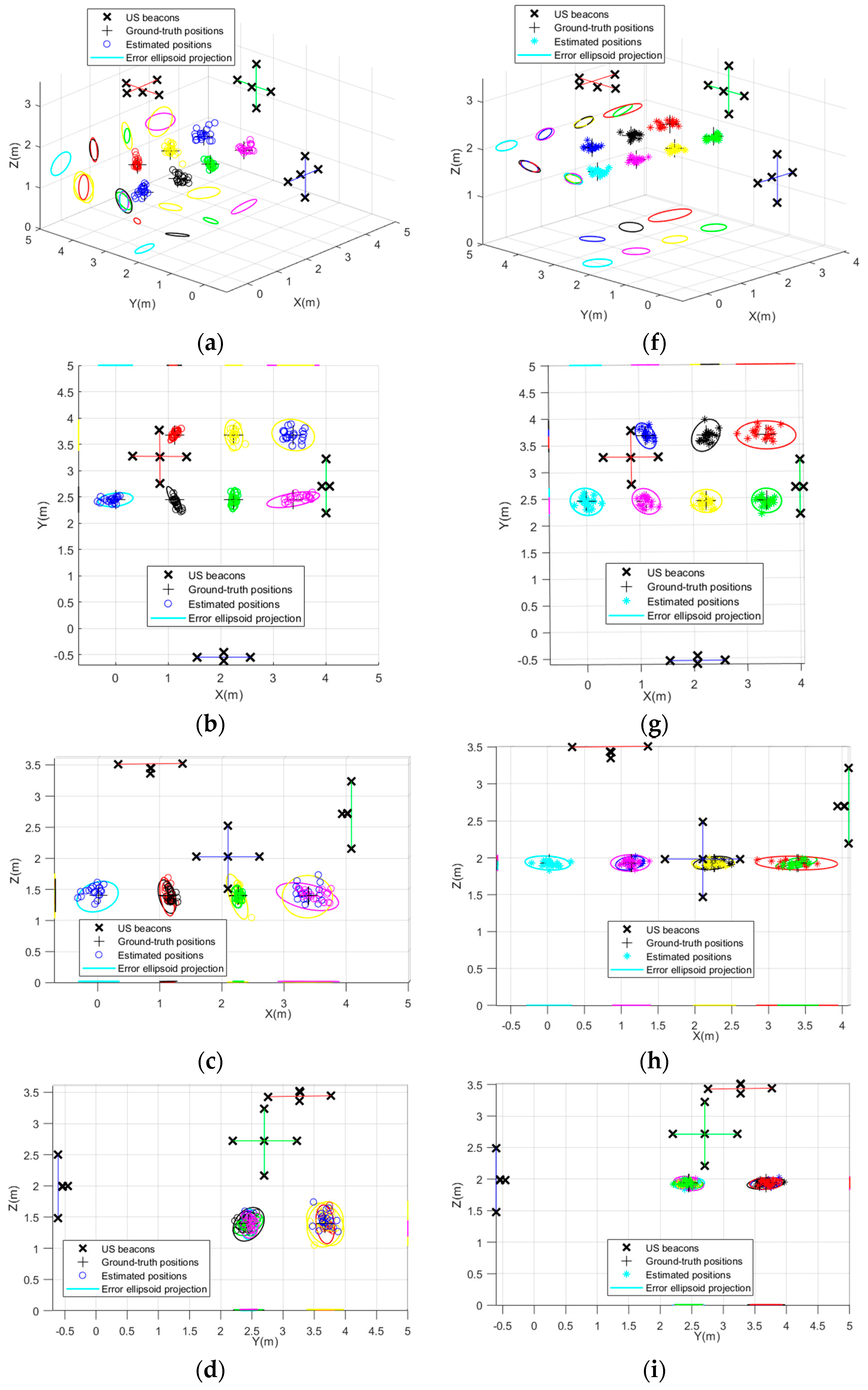
Figure 13.
Experimental results for the tested points P1–P7 for both heights, z1 = 1.35 m on the left (a–e) and z2 = 1.93 m on the right (f–j): successively, 3D representation of clouds of points; Y–X projections; Z–X projections; Z–Y projections; and experimental CDFs for each point after AKF fusion.


Figure 14.
Experimental results for the tested points P1–P7 for both heights, z1 = 1.35 m on the left (a–e) and z2 = 1.93 m on the right (f–h): successively, 3D representation of clouds of points; Y–X projections; Z–X projections; Z–Y projections; and experimental CDFs for each point after EKF fusion (σ = 0.2 m).


Table 1.
Coordinates of the central beacon B1 for every ULPS in the considered workspace.
| ULPS | Coordinates for B1 (m) |
|---|---|
| ULPS-1 | (0.84, 3.267, 3.351) |
| ULPS-2 | (2.06, −0.458, 1.980) |
| ULPS-3 | (3.92, 2.7, 2.7) |
Table 2.
Positioning errors (m) in 90% of cases for the considered positions P1–P7 at z1 = 1.35 m and z2 = 1.93 m, when the ULPSs operate independently.
Table 2.
Positioning errors (m) in 90% of cases for the considered positions P1–P7 at z1 = 1.35 m and z2 = 1.93 m, when the ULPSs operate independently.
| Positions | z1 | z2 | ||||
|---|---|---|---|---|---|---|
| ULPS-1 | ULPS-2 | ULPS-3 | ULPS-1 | ULPS-2 | ULPS-3 | |
| P1 | 0.543 | 1.757 | 2.084 | 0.783 | 1.098 | 3.57 |
| P2 | 0.476 | 0.97 | 2.57 | 0.771 | 0.844 | 1.192 |
| P3 | 0.90 | 1.041 | 1.95 | 0.919 | 1.173 | 1.128 |
| P4 | 1.098 | 1.008 | 0.215 | 1.37 | 1.326 | 0.682 |
| P5 | 2.282 | 2.203 | 3.096 | 2.27 | 2.591 | 2.249 |
| P6 | 0.546 | 1.817 | 1.109 | 0.807 | 1.855 | 0.68 |
| P7 | 2.879 | 2.557 | 2.457 | 3.086 | 2.68 | 2.484 |
Table 3.
Mean positioning errors and standard deviations for points P1–P7 at z1 = 1.35 m and z2 = 1.93 m after the LKF fusion.
Table 3.
Mean positioning errors and standard deviations for points P1–P7 at z1 = 1.35 m and z2 = 1.93 m after the LKF fusion.
| Points | z1 | z2 | ||||||||||
|---|---|---|---|---|---|---|---|---|---|---|---|---|
| Mean Error (m) | Std Deviation (m) | Mean Error (m) | Std Deviation (m) | |||||||||
| x | y | z | x | y | z | x | y | z | x | y | z | |
| P1 | 0.120 | 0.068 | 0.109 | 0.122 | 0.062 | 0.122 | 0.090 | 0.061 | 0.090 | 0.082 | 0.045 | 0.082 |
| P2 | 0.107 | 0.083 | 0.161 | 0.300 | 0.064 | 0.300 | 0.089 | 0.036 | 0.089 | 0.298 | 0.035 | 0.298 |
| P3 | 0.041 | 0.190 | 0.041 | 0.041 | 0.192 | 0.041 | 0.042 | 0.024 | 0.042 | 0.036 | 0.014 | 0.036 |
| P4 | 0.404 | 0.044 | 0.233 | 0.258 | 0.026 | 0.258 | 0.204 | 0.028 | 0.204 | 0.186 | 0.023 | 0.186 |
| P5 | 0.030 | 0.124 | 0.186 | 0.021 | 0.128 | 0.021 | 0.017 | 0.028 | 0.017 | 0.012 | 0.023 | 0.012 |
| P6 | 0.103 | 0.034 | 0.180 | 0.080 | 0.033 | 0.080 | 0.052 | 0.081 | 0.052 | 0.036 | 0.057 | 0.036 |
| P7 | 0.232 | 0.233 | 0.271 | 0.263 | 0.289 | 0.263 | 0.114 | 0.089 | 0.114 | 0.105 | 0.062 | 0.105 |
Table 4.
Positioning errors (m) for P1–P7 in 90% of the cases after the LKF fusion.
| Points | z1 | z2 |
|---|---|---|
| P1 | 0.208 | 0.134 |
| P2 | 0.221 | 0.054 |
| P3 | 0.245 | 0.061 |
| P4 | 0.522 | 0.292 |
| P5 | 0.349 | 0.071 |
| P6 | 0.322 | 0.108 |
| P7 | 0.751 | 0.168 |
Table 5.
Mean positioning errors and standard deviations for points P1–P7 at z1 = 1.35 m and z2 = 1.93 m after an AKF fusion.
Table 5.
Mean positioning errors and standard deviations for points P1–P7 at z1 = 1.35 m and z2 = 1.93 m after an AKF fusion.
| Points | z1 | z2 | ||||||||||
|---|---|---|---|---|---|---|---|---|---|---|---|---|
| Mean Error (m) | Std Deviation (m) | Mean Error (m) | Std Deviation (m) | |||||||||
| x | y | z | x | y | z | x | y | z | x | y | z | |
| P1 | 0.121 | 0.066 | 0.110 | 0.088 | 0.036 | 0.074 | 0.116 | 0.086 | 0.045 | 0.139 | 0.044 | 0.027 |
| P2 | 0.082 | 0.065 | 0.124 | 0.243 | 0.051 | 0.102 | 0.071 | 0.043 | 0.024 | 0.119 | 0.059 | 0.042 |
| P3 | 0.031 | 0.103 | 0.099 | 0.029 | 0.118 | 0.058 | 0.036 | 0.032 | 0.023 | 0.223 | 0.030 | 0.016 |
| P4 | 0.270 | 0.032 | 0.131 | 0.295 | 0.025 | 0.117 | 0.173 | 0.031 | 0.028 | 0.039 | 0.025 | 0.025 |
| P5 | 0.031 | 0.138 | 0.231 | 0.023 | 0.074 | 0.115 | 0.017 | 0.022 | 0.036 | 0.187 | 0.023 | 0.016 |
| P6 | 0.149 | 0.061 | 0.280 | 0.141 | 0.061 | 0.250 | 0.028 | 0.075 | 0.032 | 0.012 | 0.013 | 0.024 |
| P7 | 0.178 | 0.210 | 0.255 | 0.221 | 0.272 | 0.303 | 0.153 | 0.086 | 0.027 | 0.120 | 0.066 | 0.026 |
Table 6.
Positioning error (m) for points P1–P7 in 90% of cases after an AKF.
| Points | z1 | z2 |
|---|---|---|
| P1 | 0.205 | 0.169 |
| P2 | 0.208 | 0.073 |
| P3 | 0.139 | 0.072 |
| P4 | 0.306 | 0.168 |
| P5 | 0.306 | 0.054 |
| P6 | 0.426 | 0.111 |
| P7 | 0.622 | 0.214 |
Table 7.
Mean positioning errors and standard deviations for an EKF (σw = 0.2 m).
| Points | z1 | z2 | ||||||||||
|---|---|---|---|---|---|---|---|---|---|---|---|---|
| Mean Error (m) | Std Deviation (m) | Mean Error (m) | Std Deviation (m) | |||||||||
| x | y | z | x | y | z | x | y | z | x | y | z | |
| P1 | 0.163 | 0.098 | 0.117 | 0.021 | 0.020 | 0.021 | 0.084 | 0.079 | 0.029 | 0.026 | 0.053 | 0.027 |
| P2 | 0.119 | 0.034 | 0.076 | 0.030 | 0.021 | 0.026 | 0.109 | 0.066 | 0.041 | 0.029 | 0.045 | 0.027 |
| P3 | 0.143 | 0.112 | 0.131 | 0.027 | 0.046 | 0.032 | 0.053 | 0.097 | 0.069 | 0.035 | 0.033 | 0.058 |
| P4 | 0.108 | 0.052 | 0.223 | 0.028 | 0.013 | 0.076 | 0.076 | 0.179 | 0.051 | 0.041 | 0.030 | 0.024 |
| P5 | 0.065 | 0.037 | 0.210 | 0.027 | 0.018 | 0.030 | 0.064 | 0.095 | 0.057 | 0.038 | 0.049 | 0.037 |
| P6 | 0.070 | 0.029 | 0.216 | 0.020 | 0.024 | 0.046 | 0.078 | 0.091 | 0.047 | 0.043 | 0.044 | 0.042 |
| P7 | 0.223 | 0.069 | 0.267 | 0.040 | 0.040 | 0.041 | 0.070 | 0.155 | 0.102 | 0.043 | 0.041 | 0.067 |
Table 8.
Summary of errors for 90% of the estimated positions for the different considered fusion methods.
Table 8.
Summary of errors for 90% of the estimated positions for the different considered fusion methods.
| Positioning Error (m) | z1 | z2 | |||||
|---|---|---|---|---|---|---|---|
| Min | Max | Mean | Min | Max | Mean | ||
| Loosely coupled fusion | LKF | 0.5 | 0.78 | 0.5 | 0.1 | 0.4 | 0.25 |
| AKF | 0.2 | 0.82 | 0.4 | 0.1 | 0.34 | 0.2 | |
| Tightly coupled fusion | EKF | 0.107 | 0.3 | 0.22 | 0.105 | 0.2 | 0.152 |
Table 9.
Positioning error containing 90% of the estimated positions at z1 = 1.35 m and z2 = 1.93 m when the three ULPSs operated independently.
Table 9.
Positioning error containing 90% of the estimated positions at z1 = 1.35 m and z2 = 1.93 m when the three ULPSs operated independently.
| Points | z1 | z2 | ||||
|---|---|---|---|---|---|---|
| ULPS-1 | ULPS-2 | ULPS-3 | ULPS-1 | ULPS-2 | ULPS-3 | |
| P1 | 0.608 | 2.061 | 1.383 | 0.297 | 3.318 | 4.367 |
| P2 | 0.551 | 1.165 | 1.246 | 0.556 | 1.012 | 1.293 |
| P3 | 0.892 | 0.872 | 1.010 | 0.53 | 0.762 | 0.494 |
| P4 | 2.313 | 0.998 | 0.823 | 1.134 | 1.057 | 0.187 |
| P5 | 0.472 | 0.788 | 2.578 | 0.204 | 2.072 | 1.091 |
| P6 | 1.482 | 1.165 | 1.010 | 1.686 | 1.65 | 0.527 |
| P7 | 2.130 | 1.863 | 0.679 | 2.049 | 1.19 | 0.542 |
Table 10.
Mean errors and standard deviations of estimated positions when applying the LKF at z1 = 1.35 m and z2 = 1.93 m for the test points (P1–P7).
Table 10.
Mean errors and standard deviations of estimated positions when applying the LKF at z1 = 1.35 m and z2 = 1.93 m for the test points (P1–P7).
| Positions | z1 | z2 | ||||||||||
|---|---|---|---|---|---|---|---|---|---|---|---|---|
| Mean Error (m) | Std Deviation (m) | Mean Error (m) | Std Deviation (m) | |||||||||
| x | y | z | x | y | z | x | y | z | x | y | z | |
| P1 | 0.248 | 0.093 | 0.658 | 0.223 | 0.054 | 0.298 | 0.074 | 0.071 | 0.110 | 0.080 | 0.053 | 0.089 |
| P2 | 0.083 | 0.254 | 0.705 | 0.033 | 0.071 | 0.188 | 0.070 | 0.073 | 0.079 | 0.061 | 0.042 | 0.055 |
| P3 | 0.140 | 0.266 | 0.685 | 0.149 | 0.133 | 0.083 | 0.140 | 0.064 | 0.071 | 0.238 | 0.056 | 0.056 |
| P4 | 0.192 | 0.175 | 0.608 | 0.165 | 0.106 | 0.244 | 0.083 | 0.061 | 0.119 | 0.059 | 0.059 | 0.115 |
| P5 | 0.018 | 0.016 | 0.418 | 0.011 | 0.012 | 0.185 | 0.079 | 0.068 | 0.176 | 0.061 | 0.058 | 0.118 |
| P6 | 0.132 | 0.131 | 0.640 | 0.191 | 0.078 | 0.115 | 0.165 | 0.082 | 0.074 | 0.140 | 0.069 | 0.050 |
| P7 | 0.313 | 0.286 | 0.714 | 0.104 | 0.186 | 0.113 | 0.163 | 0.077 | 0.058 | 0.127 | 0.059 | 0.041 |
Table 11.
Mean errors and standard deviations of estimated positions when applying the AKF at z1 = 1.35 m and z2 = 1.93 m for the test points (P1–P7).
Table 11.
Mean errors and standard deviations of estimated positions when applying the AKF at z1 = 1.35 m and z2 = 1.93 m for the test points (P1–P7).
| Position | z1 | z2 | ||||||||||
|---|---|---|---|---|---|---|---|---|---|---|---|---|
| Mean Error (m) | Std Deviation (m) | Mean Error (m) | Std Deviation (m) | |||||||||
| x | y | z | x | y | z | x | y | z | x | y | z | |
| P1 | 0.248 | 0.093 | 0.240 | 0.223 | 0.054 | 0.202 | 0.074 | 0.071 | 0.028 | 0.080 | 0.053 | 0.021 |
| P2 | 0.083 | 0.254 | 0.177 | 0.033 | 0.071 | 0.170 | 0.070 | 0.073 | 0.033 | 0.061 | 0.042 | 0.021 |
| P3 | 0.140 | 0.266 | 0.139 | 0.149 | 0.133 | 0.083 | 0.088 | 0.064 | 0.024 | 0.053 | 0.056 | 0.016 |
| P4 | 0.192 | 0.175 | 0.206 | 0.165 | 0.106 | 0.138 | 0.083 | 0.061 | 0.023 | 0.059 | 0.059 | 0.019 |
| P5 | 0.018 | 0.016 | 0.198 | 0.011 | 0.012 | 0.100 | 0.052 | 0.068 | 0.024 | 0.050 | 0.058 | 0.023 |
| P6 | 0.132 | 0.131 | 0.126 | 0.191 | 0.078 | 0.076 | 0.072 | 0.082 | 0.025 | 0.067 | 0.061 | 0.018 |
| P7 | 0.313 | 0.286 | 0.174 | 0.104 | 0.186 | 0.103 | 0.163 | 0.077 | 0.028 | 0.127 | 0.059 | 0.016 |
Table 12.
Mean errors and standard deviations for three ULPSs and a single EKF (σw = 0.2 m).
| Position | z1 | z2 | ||||||||||
|---|---|---|---|---|---|---|---|---|---|---|---|---|
| Mean Error (m) | Std Deviation (m) | Mean Error (m) | Std Deviation (m) | |||||||||
| x | y | z | x | y | z | x | y | z | x | y | z | |
| P1 | 0.143 | 0.076 | 0.060 | 0.067 | 0.062 | 0.038 | 0.061 | 0.009 | 0.037 | 0.006 | 0.004 | 0.006 |
| P2 | 0.135 | 0.104 | 0.176 | 0.080 | 0.071 | 0.151 | 0.074 | 0.062 | 0.027 | 0.008 | 0.009 | 0.007 |
| P3 | 0.121 | 0.168 | 0.111 | 0.119 | 0.097 | 0.079 | 0.087 | 0.090 | 0.147 | 0.010 | 0.010 | 0.008 |
| P4 | 0.140 | 0.197 | 0.157 | 0.100 | 0.136 | 0.112 | 0.108 | 0.015 | 0.153 | 0.006 | 0.008 | 0.010 |
| P5 | 0.129 | 0.204 | 0.155 | 0.076 | 0.101 | 0.103 | 0.156 | 0.156 | 0.095 | 0.012 | 0.009 | 0.007 |
| P6 | 0.102 | 0.337 | 0.135 | 0.092 | 0.142 | 0.117 | 0.105 | 0.098 | 0.105 | 0.009 | 0.011 | 0.012 |
| P7 | 0.225 | 0.397 | 0.097 | 0.109 | 0.148 | 0.066 | 0.110 | 0.114 | 0.110 | 0.008 | 0.007 | 0.010 |
Table 13.
Summary of the CDF errors for 90% of the estimated positions and the availability of estimates at z1 and z2.
Table 13.
Summary of the CDF errors for 90% of the estimated positions and the availability of estimates at z1 and z2.
| CDF Error (m) | z1 | z2 | % of Positions | |||||
|---|---|---|---|---|---|---|---|---|
| Min | Max | Mean | Min | Max | Mean | |||
| Loosely coupled | LKF | 0.48 | 0.76 | 0.68 | 0.16 | 0.283 | 0.211 | 90% |
| AKF | 0.221 | 0.574 | 0.354 | 0.116 | 0.227 | 0.157 | 90% | |
| Tightly coupled | EKF | 0.182 | 0.46 | 0.302 | 0.105 | 0.301 | 0.151 | 100% |
Publisher’s Note: MDPI stays neutral with regard to jurisdictional claims in published maps and institutional affiliations. |
© 2021 by the authors. Licensee MDPI, Basel, Switzerland. This article is an open access article distributed under the terms and conditions of the Creative Commons Attribution (CC BY) license (https://creativecommons.org/licenses/by/4.0/).
Share and Cite
MDPI and ACS Style
Mannay, K.; Ureña, J.; Hernández, Á.; Villadangos, J.M.; Machhout, M.; Aguili, T. Evaluation of Multi-Sensor Fusion Methods for Ultrasonic Indoor Positioning. Appl. Sci. 2021, 11, 6805. https://doi.org/10.3390/app11156805
AMA Style
Mannay K, Ureña J, Hernández Á, Villadangos JM, Machhout M, Aguili T. Evaluation of Multi-Sensor Fusion Methods for Ultrasonic Indoor Positioning. Applied Sciences. 2021; 11(15):6805. https://doi.org/10.3390/app11156805
Chicago/Turabian StyleMannay, Khaoula, Jesús Ureña, Álvaro Hernández, José M. Villadangos, Mohsen Machhout, and Taoufik Aguili. 2021. "Evaluation of Multi-Sensor Fusion Methods for Ultrasonic Indoor Positioning" Applied Sciences 11, no. 15: 6805. https://doi.org/10.3390/app11156805
Note that from the first issue of 2016, this journal uses article numbers instead of page numbers. See further details here.