
Effect of Eigenmode Frequency on Loss Tangent Atomic Force Microscopy Measurements


Mechanical Engineering Department at Widener University, One University Place, Chester, PA 19013, USA
*
Author to whom correspondence should be addressed.
Appl. Sci. 2021, 11(15), 6813; https://doi.org/10.3390/app11156813
Submission received: 30 June 2021
/
Revised: 14 July 2021
/
Accepted: 21 July 2021
/
Published: 24 July 2021
(This article belongs to the Special Issue Advances in Surface Modification of the Materials)
Abstract
:Featured Application
Micro-scale characterization of viscoelastic materials with atomic force microscopy.
Abstract
Atomic Force Microscopy (AFM) is no longer used as a nanotechnology tool responsible for topography imaging. However, it is widely used in different fields to measure various types of material properties, such as mechanical, electrical, magnetic, or chemical properties. One of the recently developed characterization techniques is known as loss tangent. In loss tangent AFM, the AFM cantilever is excited, similar to amplitude modulation AFM (also known as tapping mode); however, the observable aspects are used to extract dissipative and conservative energies per cycle of oscillation. The ratio of dissipation to stored energy is defined as . This value can provide useful information about the sample under study, such as how viscoelastic or elastic the material is. One of the main advantages of the technique is the fact that it can be carried out by any AFM equipped with basic dynamic AFM characterization. However, this technique lacks some important experimental guidelines. Although there have been many studies in the past years on the effect of oscillation amplitude, tip radius, or environmental factors during the loss tangent measurements, there is still a need to investigate the effect of excitation frequency during measurements. In this paper, we studied four different sets of samples, performing loss tangent measurements with both first and second eigenmode frequencies. It is found that performing these measurements with higher eigenmode is advantageous, minimizing the tip penetration through the surface and therefore minimizing the error in loss tangent measurements due to humidity or artificial dissipations that are not dependent on the actual sample surface.
1. Introduction
Since the invention of atomic force microscopy, amplitude modulation (AM-AFM) is known as the most common mode of imaging various types of samples in dynamic mode measurements of AFM. Besides the relative ease of calculating measurements, AM-AFM can provide a wide range of information, such as topography, stiffness, dissipation, and material composition in a single-pass measurement [1,2,3]. Unlike contact mode AFM, AM-AFM provides topographical measurement, with a possibility of compositional mapping that includes a lower chance of damaging surfaces [1,2,4]. In a conventional AM-AFM measurement, the cantilever is excited at, or near, resonance frequency (i.e., typically the first eigenmode frequency) while the tip–surface distance is modulated by either moving the sample in Z direction or moving the base of the cantilever to maintain a constant oscillation amplitude. The amplitude signal is used to extract the topographical measurement while the phase signal is used for material characterization purposes [2].
Although AM-AFM can provide some immediate advantages compared to contact mode or other advanced dynamic modes of AFM, it does not provide a direct quantitative measurement of mechanical properties of materials, especially if they are viscoelastic polymers. During the past few decades, there have many studies to show how one can extract quantitative properties of materials from just the amplitude and phase signals of AM-AFM images [5,6,7]. Firstly, these attempts require extensive mathematical models to be used to calculate the material properties. Secondly, they require measurements at various oscillation amplitudes, setpoint values, and different tip velocities. Since most of the samples that are of high importance in these measurements are delicate samples, multiple measurements in the same area over the surface might cause permanent damages. Therefore, it remains challenging to obtain reliable and consistent material properties from AM-AFM measurements. A relatively new approach has focused on distinguishing conservative and dissipative tip–sample force interactions in AM-AFM [8,9]. In doing so, quantities known as virial and dissipated were defined and used in different studies [6,8,10]. Although it is still unknown how one can directly relate virial to a mechanical property of a surface, virial is commonly related to the stiffness of tip–sample forces observed by the cantilever while dissipated power is known as energy loss in a full cycle [7]. This method can separate the effect of each category of forces; however, it requires accurate measurements of oscillation amplitude and probe characteristics to be a reliable measurement technique. Additionally, if a higher eigenmode is used to observe compositional contrasts in phase channel, the calibration process becomes more sophisticated.
Recently, studies were done that implemented a more general and straightforward method known as loss tangent () measurements [11,12]. The quantity is a dimensionless value that is processed as an image (i.e., observable) during a conventional AM-AFM mode. This quantity is defined as the ratio of the dissipative and conservative energy contributions during each oscillation cycle of the probe. Although the value does not provide separate quantities for conservative and dissipative energies, the ratio can provide insightful information about the sample under study. Based on the study by Cleveland et al., it was found that the dissipated power of the cantilever driven at the fundamental resonant frequency and the phase lag angle can be related as shown in Equation (1) [8]:
where is the free oscillation amplitude, is the resonant frequency (i.e., first eigenmode in this case), is the spring constant of the cantilever, and is the quality factor. The total energy dissipated per oscillatory cycle of the cantilever can be written as Equation (2).
where is the period of an oscillation cycle. Although there can be many sources for dissipation of energy within an oscillation (such as capillary forces, electrostatic charges, or magnetic forces), in a controlled setting, it is assumed to be due to the viscoelastic interaction and the hysteresis in the surface adhesion interaction between the tip and surface. Therefore, the dissipated power can be also written as and the stored power of the oscillating cantilever can be written as Because of this relationship, Proksch and Yablon showed that the can be directly found by amplitude and phase signals, so it can be written as [11]:
It should be noted that the ratio of instantaneous oscillation amplitude () to free oscillation amplitude () make this relationship independent of actual amplitude values in length units. Therefore, Equation (3) can be re-written as the following, where and represent the voltage values of instantaneous oscillation amplitude and free oscillation amplitude, respectively.
It should be noted that based on the Equation shown in (4), the can be found without the need for accurate calibration of actual amplitude values. Although there are many studies that have done different types of analysis on this topic, there is still a gap in the field to understand the true effect of tip–velocity (i.e., excitation frequency) on the observable aspects in loss tangent AM-AFM measurements. Procksh et al. have examined the effect of oscillation amplitudes [11]. Nguyen et al. showed that the AM-AFM loss tangent measurements overestimated the values compared to bulk measurements [13]. In a recent study, Nguyen H. K. et al. have also investigated the effect of tip radius on the measured values [14]. It was found that ultra-sharp tips are advantageous to eliminating the unwanted dissipative processes. In this study, we focus on the effect of excitation frequency and the penetration depth caused by the tip trajectory on different types of materials and compare them with published bulk material properties. Yablon et al. have suggested using cantilevers with frequencies over 300 kHz [12,13,15]. A practical method to do so is using the higher eigenmode of a typical AM-AFM cantilever to achieve this guideline. However, it is still unknown how the penetration of the tip into soft matter can play a role in the observable aspects of loss tangent measurements.
2. Materials and Methods
Materials: In this study, four different sample systems were used to investigate the effect of tip penetration due to higher excitation frequency in loss tangent AFM. The first set of samples was a Sapphire surface manufactured by Bruker (known as PFQNM-SMPKIT-12M). This surface provided a flat and stiff surface for AFM measurements. The second sample was a blend of Polystyrene (PS) and Polyolefin Elastomer (ethylene-octene copolymer, LDPE), which were spin-coated on a silicon substrate with 1500 RPM for 60 seconds to create a thin film with varying material properties. The PS regions of the sample had elastic modulus numbers around 2 GPa while the copolymer regions had elastic modulus numbers around 0.1 GPa. Therefore, it could provide a clear contrast in material composition studies by AFM. The third sample was a single-polymer thin film. Polystyrene with 33 kDA molecular weight diluted into 2.5 wt% in THF was used, which was spin-coated onto a silicon wafer at 1400 rpm for 60 seconds. We selected a polystyrene of low molecular weight to prepare a sample that displayed time-dependent behavior within the deformational timescale in our studies (previous studies have quantified the dependence of characteristic times on the molecular weight of polystyrene [16]. The humidity was increased to above 60% in order to create islands that could expose the stiff substrate. This could provide a drastic material change in our sample which is suitable for the purpose of this study. The fourth sample was Teflon, more commonly and widely known by the name Polytetrafluoroethylene (PTFE), a fluorocarbon solid. Teflon has one of the lowest coefficients of friction, which is why it is widely used in many different industrial applications.
AFM Measurements: All measurements were operated in AM-AFM mode using MFP3D Origin AFM (Asylum Research, Oxford Instruments, USA) in air conditions (~299 K, relative humidity of ~%30). All the measurements were done using the same type of cantilever to provide consistency in measurements. Between each measurement, the tip of the cantilever was monitored to ensure there was no contamination from previous studies. The most common type of cantilever available commercially for topography and viscoelasticity measurements of soft samples is AC240TS-R3 manufactured by Olympus. This cantilever had the first eigenmode resonance frequency of and The tip radius was measured by the manufacturer to be around . The nominal spring constant was measured to be 2.3 N/m.
3. Results
We investigated the effect of excitation frequency on the tip penetration through different surfaces in the context of loss tangent AFM measurement. It is known that higher excitation frequencies can cause higher tip penetration through surfaces [16,17]. As mentioned, the recent studies in loss tangent AFM field have shown that the higher tip radius can cause higher dissipation, hence, higher loss tangent values. However, these studies have not considered the effect of tip penetration on the surface and the consequence of effective tip radius on these measurements.
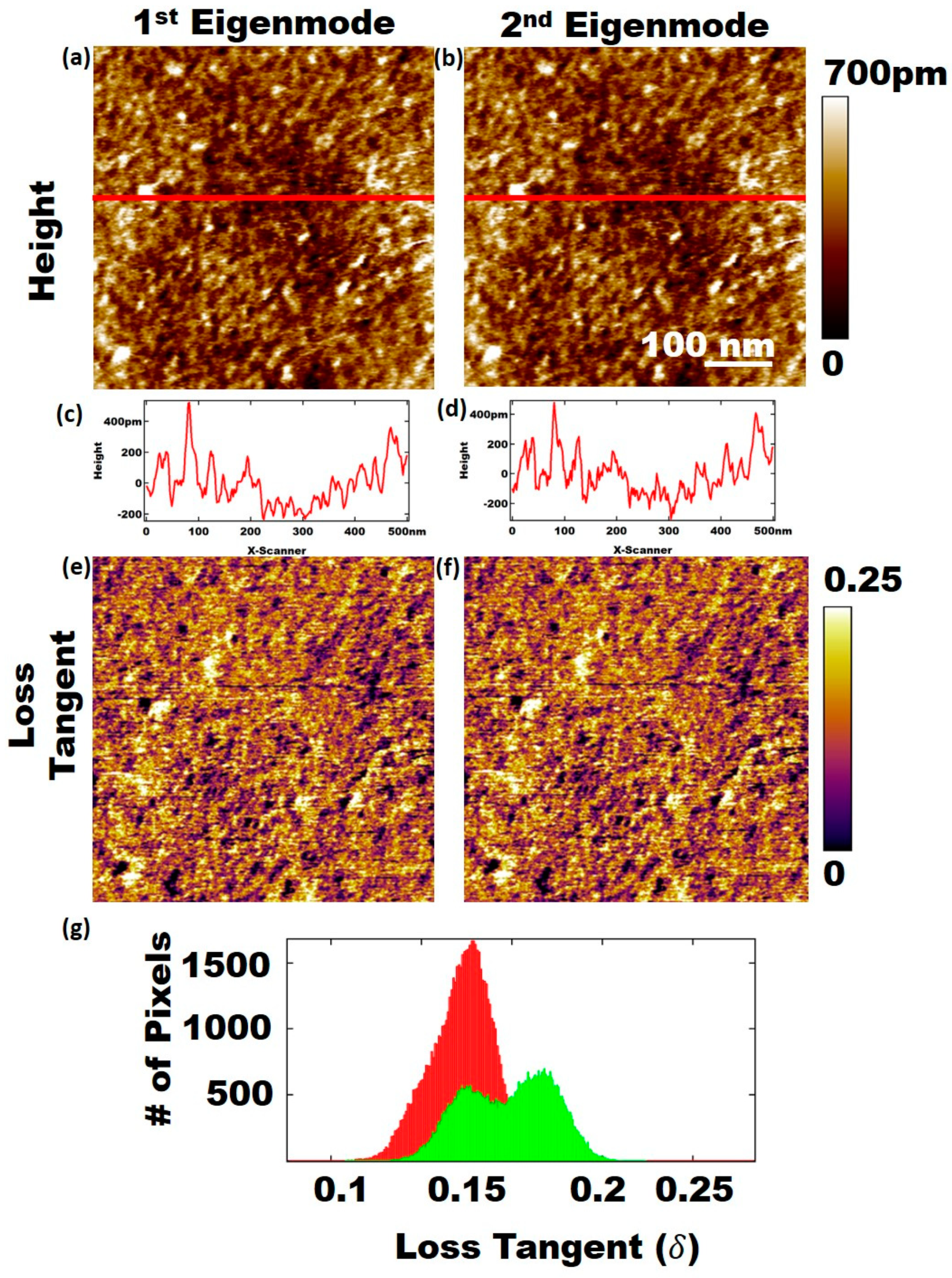
In this work, we examined different types of samples in a systematic way in order to experimentally find the effect of these parameters on loss tangent AFM measurements. Figure 1 represents two sets of experiments using AM-AFM mode, where the amplitude and phase signals are used to generate the loss tangent images. The first round of measurements, shown in the left column of Figure 1, was conducted by exciting the cantilever in AM-AFM with its first eigenmode frequency. In contrast, the second round of measurements, shown in the right column of Figure 1, was performed by exciting the cantilever in AM-AFM with its second eigenmode frequency. The sample understudy in Figure 1 is Sapphire, which is known as a flat and stiff surface. Therefore, one can assume there is no tip penetration in these studies due to surface softness. Figure 1a,b represent topography (i.e., height) images of the same area of the sample conducted with 1st and 2nd eigenmode, respectively. Since the sample is relatively flat, scan lines are shown in Figure 1c,d in order to quantitatively compare the differences. Besides the fact that Figure 1d has a larger number of peaks in the scan line (which can be due to imaging conditions), Figure 1c,d show relatively similar topographies as expected. Figure 1e and f show the phase images of the same measurements explained in Figure 1a,b. Although qualitatively they seem similar, the phase images are used to generate loss tangent measurements, which are represented by a histogram in Figure 1g. In this study, it is clear that when we were imaging with the first eigenmode frequency, higher values of were observed. Additionally, there appear to be two peaks of loss tangent values shown in green histograms of Figure 1g when imaged by the first eigenmode. This observation is linked to the thin layer of humidity that can exist during measurements. Although there are no tip penetrations on this sample, due to higher stiffness of the second eigenmode, the thin layer of humidity can be compressed (or not observed) by the tip–sample force interactions. Consequently, a single peak of loss tangent values is observable for the second eigenmode, which is less dissipative as well.
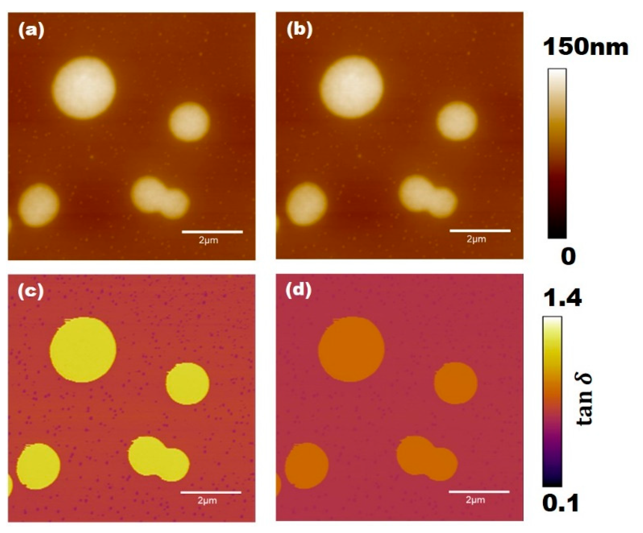
In order to study the effect of tip penetration, we conducted a similar study on a co-polymer sample system (PS-LDPE). PS has an elastic modulus around 2 GPa while LDPE is known to be a softer polymer with 0.1 GPa. This sample allows us to know if there is any difference with the way polymers respond to loss tangent AFM imaging with the first or second eigenmode frequencies. Figure 2a,b show the same area on the sample that used the 1st eigenmode and 2nd eigenmode excitation frequencies, respectively. Figure 2c,d represent the loss tangent AFM image done by 1st and 2nd eigenmode excitation frequencies, respectively. It is clear from these images that when we excite the cantilever with higher frequency, we see less dissipation compared to when we used the first eigenmode frequency. Although the second eigenmode frequency has a higher stiffness, the tip penetration is lower. Therefore, the effective tip radius results in less dissipation. It should be mentioned that this finding is consistent with the recent findings presented in Nikfarjam et al.’s work as well related to the tip penetration by higher eigenmodes [16].
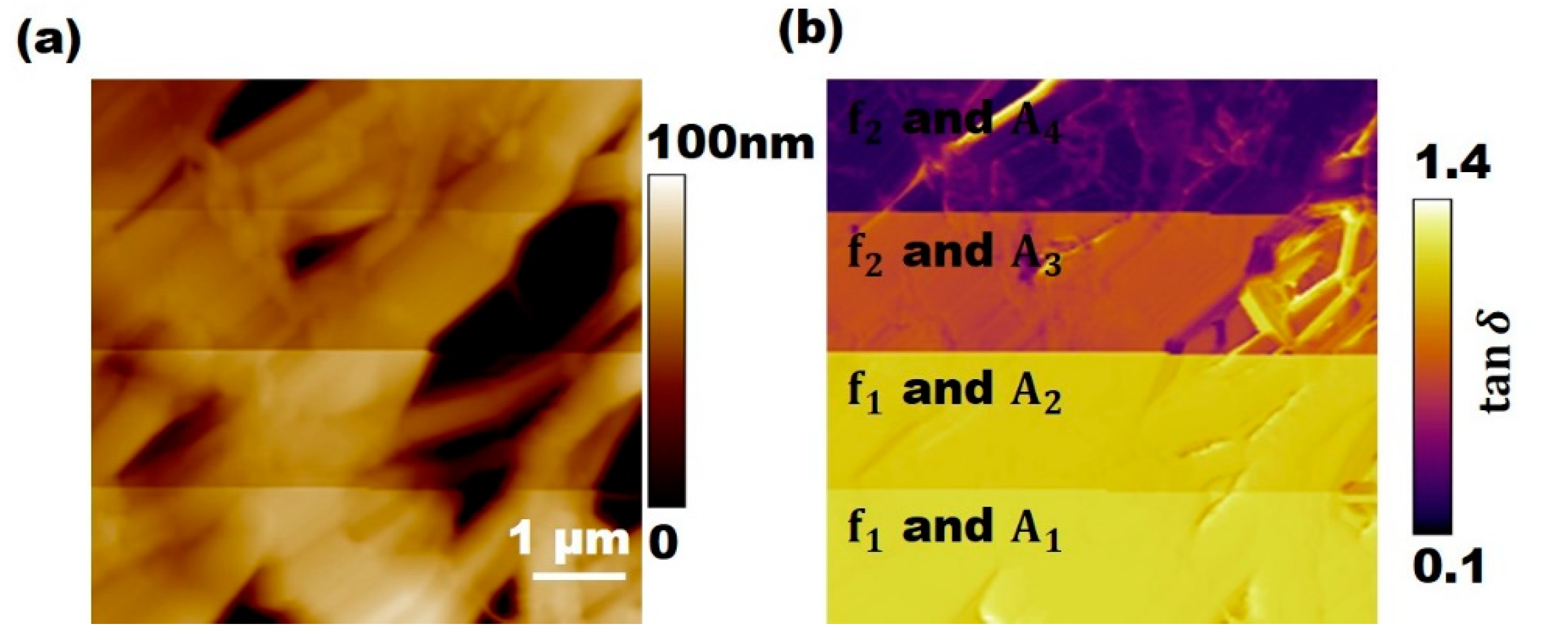
Although Figure 1 and Figure 2 provided a useful insight in regard to selection of excitation frequency for loss tangent AFM images, questions remain about the effect of the oscillation amplitudes, which have a more important role in defining the tip penetrations on samples. In order to systematically study this effect, a Teflon tape is stretched and mounted on a glass slide. Additionally, we performed four different sets of experiments. For each excitation frequency (i.e., either first or second in this case), two different free oscillation amplitudes are selected so that the product of stiffness and oscillation amplitudes stay constant (i.e., ). This is done by understanding the equation of motion of the cantilever in normalized form [16,18,19]:
where is the free amplitude, is the dimensionless tip position with respect to the cantilever base, is the dimensionless tip–sample distance () where is the position of the cantilever above the sample, is the dimensionless time, is the cantilever force constant, and is the tip–sample interaction force. We made the substitution [2], where is the amplitude of the excitation force, and we combined the damping and excitation terms with the factor . The last term on the right-hand side represents the tip–sample force interaction that is normalized by the product of . Therefore, depending on the excitation frequency at which we are shaking the cantilever, its spring constant can change. However, the effect of tip–sample force interactions on the dynamics of the cantilever can be controlled by adjusting the oscillation amplitude. Figure 3 represents a set of studies where the effect of excitation frequency and oscillation amplitude on the measured loss tangent values of a PTFE sample is shown.
Figure 3a represents the topography or height image of the measurements. From the bottom to the top of the image, the imaging conditions have been modified. The lowest portion of the figure represents the measurements using first eigenmode frequency and oscillation amplitude of 50 nm. In the second portion of the image, the excitation frequency is kept constant; however, the oscillation amplitude is increased to 100 nm. Based on this change, we can see that the color in the loss tangent shows a similar result compared to previous case. However, when the excitation frequency is changed to the second eigenmode frequency, the loss tangent value is decreased (the colors in Figure 3b get darker). This trend continues when we increased the oscillation amplitude as well. This is an indication that the tip is penetrating less into the surface and therefore dissipating less energy. Based on this study, it can be concluded that if one is after loss tangent measurements of soft samples, measuring with the higher eigenmode frequencies while controlling the oscillation amplitudes can be advantageous. This can be extremely important for imaging sensitive samples, such as biological cells.
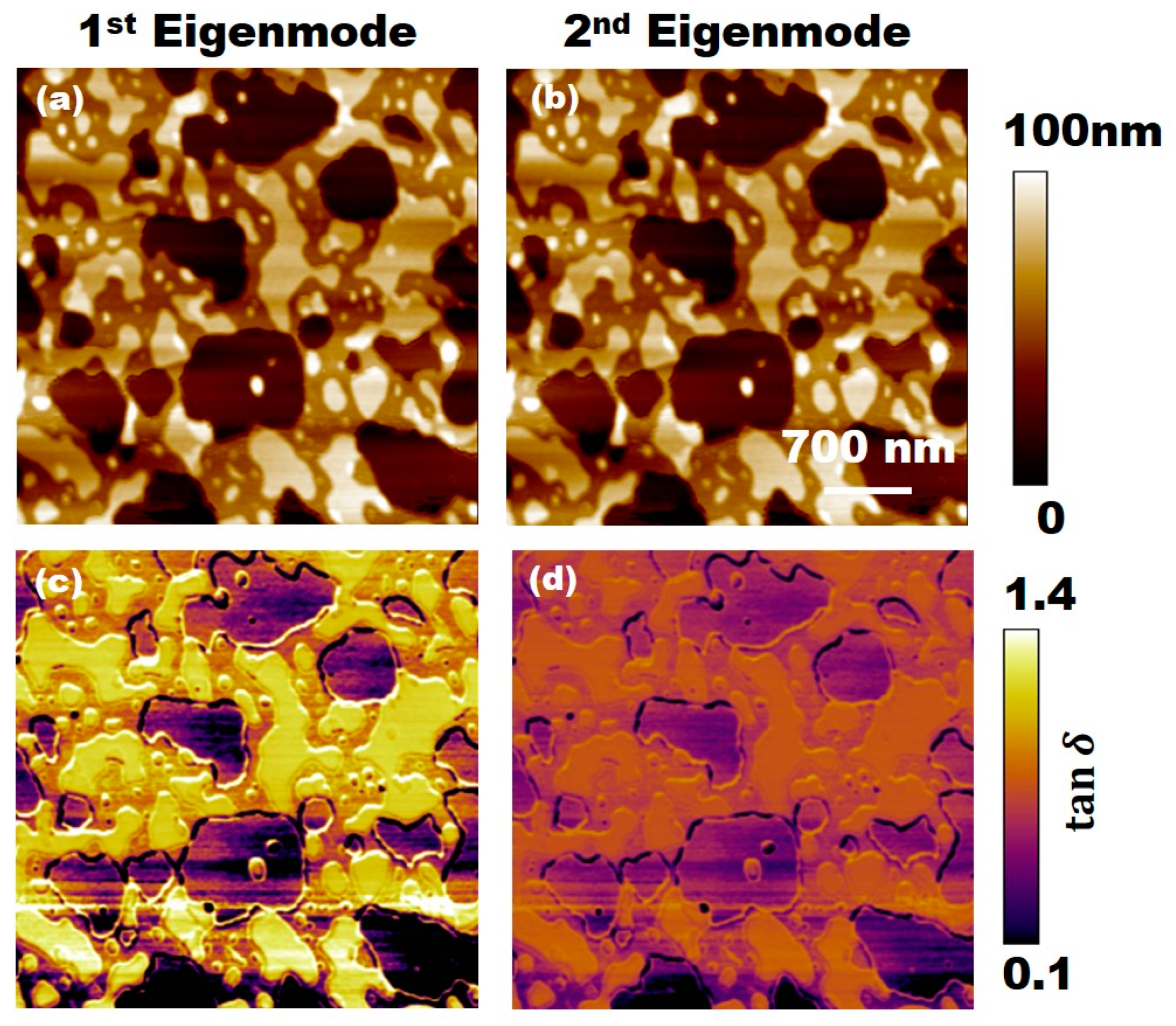
In order to have a reliable characterization technique by AFM, a common approach is studying the contrast in the observable aspects on a sample where a portion of the sample can be considered as reference material. Figure 4 provides this set for this study. The sample shown in Figure 4 is a thin film of PS polymer that is intentionally spin-coated on a silicon wafer at high humidity to create the islands shown. The high humidity has caused some portions of the silicon wafer to be exposed during the measurements as a reference material that has very high stiffness and very low viscoelasticity. Therefore, we should expect a theoretical value of for those portions to be close to zero. The left column in Figure 4 provides the height (Figure 4a) and loss tangent image (Figure 4c) using the first eigenmode frequency while the right column in Figure 4 represents the same measurements using the second eigenmode frequency. Although there is no obvious difference in topography measurements (Figure 4a,b), there is a major difference in loss tangent images shown in Figure 4c,d. The average loss tangent value is higher on the sample when imaged by the first eigenmode frequency compared to second eigenmode frequency. It should be noted both measurements are done on the same area of the same sample; therefore, one would expect identical results. However, it is clear that the second eigenmode measurements are showing less dissipation. With that said, if the aim is to distinguish the two different samples, imaging with the first eigenmode might be better since it can provide higher contrast. However, that comes with the disadvantage of penetrating more into the surface. If a sample is soft, imaging with the first eigenmode with large oscillation amplitudes can cause surface damages. On the other hand, although the second eigenmode stiffness is higher than the first one, due to lower oscillation amplitudes, imaging with the second eigenmode can be advantageous since it has been shown it can provide less dissipation of energy and have less penetration of the surface.
4. Discussion and Conclusions
In recent years, the field of atomic force microscopy has been found to have great potential in being used as a micro- or nano-scale characterization tool that is capable of not only providing topographical information of surfaces but also about various types of material properties. However, there still exists a gap in the field to provide accurate and reliable techniques that can be used for different applications. One of the techniques recently developed is known as loss tangent AFM technique. There are many different studies that have investigated the effect of different parameters, such oscillation amplitude or tip radius, on the observable aspects of this technique. In this paper, we have focused on the effect of excitation frequency on surface penetration during measurements on soft samples. In this study, we found that although the second eigenmode has a higher spring constant than the first eigenmode, due to the fact that the oscillation amplitudes are lower, there is less chance of damaging surfaces. Therefore, with the proposed technique, one can measure loss tangent values for a surface with AFM with less dissipation due to the tip and sample penetration.
Author Contributions
Theoretical contribution done by B.E. Experiments done by D.C. Manuscript preparation done by B.E. and D.C. Both authors have read and agreed to the published version of the manuscript.
Funding
This research was partially funded by Provost’s Office of Widener University through Provost Grant and Faculty Development Grant 2020–2021.
Institutional Review Board Statement
Not applicable.
Informed Consent Statement
Not applicable.
Data Availability Statement
Not applicable.
Conflicts of Interest
The authors declare no conflict of interest.
References
- Magonov, S.N.; Elings, V.; Whangbo, M.H. Phase imaging and stiffness in tapping-mode atomic force microscopy. Surf. Sci. 1997, 375, L385–L391. [Google Scholar] [CrossRef]
- Garcia, R.; Perez, R. Dynamic atomic force microscopy methods. Surf. Sci. Rep. 2002, 47, 197–301. [Google Scholar] [CrossRef]
- Benaglia, S.; Amo, C.A.; Garcia, R. Fast quantitative and high resolution mapping of viscoelastic properties with bimodal AFM. Nanoscale 2019, 11, 15289–15297. [Google Scholar] [CrossRef] [PubMed] [Green Version]
- Garcia, R. Nanomechanical mapping of soft materials with the atomic force microscope: Methods, theory and applications. Chem. Soc. Rev. 2020, 49, 5850–5884. [Google Scholar] [CrossRef] [PubMed]
- Rodríguez, T.R.; García, R. Compositional mapping of surfaces in atomic force microscopy by excitation of the second normal mode of the microcantilever. Appl. Phys. Lett. 2004, 84, 449–451. [Google Scholar] [CrossRef]
- Diaz, A.J.; Eslami, B.; López-Guerra, E.A.; Solares, S.D. Selection of higher eigenmode amplitude based on dissipated power and virial contrast in bimodal atomic force microscopy. J. Appl. Phys. 2014, 116, 104901. [Google Scholar] [CrossRef]
- Kiracofe, D.; Raman, A.; Yablon, D. Multiple regimes of oepration bimodal AFM: Understanding the energy of cantilever eigenmodes. Beilstein J. Nanotechnol. 2013. 4, 385–393.
- Cleveland, J.P.; Anczykowski, B.; Schmid, A.E.; Elings, V.B. Energy dissipation in tapping-mode atomic force microscopy. Appl. Phys. Lett. 1998. 72, 2613–2615. [CrossRef] [Green Version]
- Melcher, J.; Xu, X.; Raman, A. Multiple impact regimes in liquid environment dynamic atomic force microscopy. Appl. Phys. Lett. 2008, 93, 093111. [Google Scholar] [CrossRef] [Green Version]
- Eslami, B.; López-Guerra, E.A.; Diaz, A.J.; Solares, S.D. Optimization of the excitation frequency for high probe sensitivity in single-eigenmode and bimodal tapping-mode AFM. Nanotechnology 2015, 26, 165703. [Google Scholar] [CrossRef] [PubMed]
- Proksch, R.; Yablon, D.G. Loss tangent imaging: Theory and simulations of repulsive-mode tapping atomic force microscopy. Appl. Phys. Lett. 2012, 100, 073106. [Google Scholar] [CrossRef]
- Yablon, D.G.; Grabowski, J.; Chakraborty, I. Measuring the loss tangent of polymer materials with atomic force microscopy based methods. Meas. Sci. Technol. 2014, 25, 055402. [Google Scholar] [CrossRef]
- Nguyen, H.K.; Ito, M.; Nakajima, K. Elastic and viscoelastic characterization of inhomogeneous polymers by bimodal atomic force microscopy. Jpn. J. Appl. Phys. 2016, 55, 08NB06. [Google Scholar] [CrossRef]
- Nguyen, H.K.; Nakajima, K. Effect of tip radius on the nanoscale viscoelastic measurement of polymers using loss tangent method in amplitude modulation AFM. Jpn. J. Appl. Phys. 2021, 60, SE1008. [Google Scholar] [CrossRef]
- Nguyen, H.K.; Ito, M.; Fujinami, S.; Nakajima, K. Viscoelasticity of Inhomogeneous Polymers Characterized by Loss Tangent Measurements Using Atomic Force Microscopy. Macromolecules 2014, 47, 7971–7977. [Google Scholar] [CrossRef]
- Nikfarjam, M.; López-Guerra, E.A.; Solares, S.D.; Eslami, B. Imaging of viscoelastic soft matter with small indentation using higher eigenmodes in single-eigenmode amplitude-modulation atomic force microscopy. Beilstein J. Nanotechnol. 2018, 9, 1116–1122. [Google Scholar] [CrossRef] [PubMed] [Green Version]
- Eslami, B.; Ebeling, D.; Solares, S.D. Trade-offs in sensitivity and sampling depth in bimodal atomic force microscopy and comparison to the trimodal case. Beilstein J. Nanotechnol. 2014, 5, 1144–1151. [Google Scholar] [CrossRef] [PubMed]
- Ebeling, D.; Solares, S.D. Bimodal atomic force microscopy driving the higher eigenmode in frequency-modulation mode: Implementation, advantages, disadvantages and comparison to the open-loop case. Beilstein J. Nanotechnol. 2013, 4, 198–207. [Google Scholar] [CrossRef] [PubMed] [Green Version]
- Ebeling, D.; Eslami, B.; Solares, S.D.J. Visualizing the subsurface of soft matter: Simultaneous topographical imaging, depth modulation, and compositional mapping with triple frequency atomic force microscopy. ACS Nano 2013, 7, 10387–10396. [Google Scholar] [CrossRef] [PubMed]
Figure 1.
Loss tangent AFM study on Sapphire samples: (a) height image using the 1st eigenmode, (b) Height image using the 2nd eigenmode, (c) topography line of image (a), (d) topography line of image (b), (e) loss tangent image using 1st eigenmode, (f) loss tangent image done by 2nd eigenmode, and (g) histograms of loss tangent. The scale bar is 100 nm. Free first amplitude was 100 nm. Free second amplitude was 20 nm. The setpoint for both of the measurements was 60% to ensure repulsive regime imaging. The first eigenmode frequency was 72 kHz and the second eigenmode frequency was 460 kHz.

Figure 2.
PS-LDPE loss tangent AFM study: (a) height image done by 1st eigenmode (b) height image done by 2nd eigenmode. (c) loss tangent image done by 1st eigenmode, and (d) loss tangent image done by 2nd eigenmode. Images are by . Free first amplitude amplitude was 100 nm. Free second amplitude was 20 nm. The setpoint for both of the measurements was 50% to ensure repulsive regime imaging. First eigenmode frequency was 70 kHz and second eigenmode frequency was 458 kHz.

Figure 3.
PTFE loss tangent AFM study: (a) topography image and (b) image. From bottom to top, the excitation frequency and free oscillation amplitudes are as follows: The scale bar is 1 .
Figure 3.
PTFE loss tangent AFM study: (a) topography image and (b) image. From bottom to top, the excitation frequency and free oscillation amplitudes are as follows: The scale bar is 1 .

Figure 4.
PS loss tangent AFM images: (a) topography image using the 1st eigenmode, (b) topography image done with 2nd eigenmode, (c) image using the 1st eigenmode, and (d) image using the 2nd eigenmode. The scale bar is 700 nm. The free oscillation amplitude of the first and second eigenmode were 100 nm and 20 nm, respectively. The setpoint for both measurements were 60% and done in repulsive regime. The first and second excitation frequencies were 70 kHz and 460 kHz, respectively.

Publisher’s Note: MDPI stays neutral with regard to jurisdictional claims in published maps and institutional affiliations. |
© 2021 by the authors. Licensee MDPI, Basel, Switzerland. This article is an open access article distributed under the terms and conditions of the Creative Commons Attribution (CC BY) license (https://creativecommons.org/licenses/by/4.0/).
Share and Cite
MDPI and ACS Style
Eslami, B.; Caputo, D. Effect of Eigenmode Frequency on Loss Tangent Atomic Force Microscopy Measurements. Appl. Sci. 2021, 11, 6813. https://doi.org/10.3390/app11156813
AMA Style
Eslami B, Caputo D. Effect of Eigenmode Frequency on Loss Tangent Atomic Force Microscopy Measurements. Applied Sciences. 2021; 11(15):6813. https://doi.org/10.3390/app11156813
Chicago/Turabian StyleEslami, Babak, and Dylan Caputo. 2021. "Effect of Eigenmode Frequency on Loss Tangent Atomic Force Microscopy Measurements" Applied Sciences 11, no. 15: 6813. https://doi.org/10.3390/app11156813
Note that from the first issue of 2016, this journal uses article numbers instead of page numbers. See further details here.