
An Imperfect Production–Inventory Model with Mixed Materials Containing Scrap Returns Based on a Circular Economy


1
Department of Statistics and Information Science, Fu Jen Catholic University, New Taipei City 242062, Taiwan
2
Department of Marketing and Logistics Management, Chaoyang University of Technology, Taichung 413310, Taiwan
3
Department of International Business, Chien Hsin University of Science and Technology, Taoyuan City 320312, Taiwan
*
Author to whom correspondence should be addressed.
Processes 2021, 9(8), 1275; https://doi.org/10.3390/pr9081275
Submission received: 24 June 2021
/
Revised: 20 July 2021
/
Accepted: 22 July 2021
/
Published: 24 July 2021
(This article belongs to the Collection Tools, Approaches and Modeling in Sustainable Supply Chain Management)
Abstract
:The implementation of scrap recovery activities has been shown to improve the financial performance of many firms, and this kind of circular economy (CE) is particularly evident in industries with green manufacturing (GM). In this paper, we consider an imperfect multiple-stage production system that manufactures paired products made from mixed materials containing scrap returns, in which the scrap returns are converted from defective products. The feed rates of scrap returns for two products are different, and the product with the higher feed rate is placed in the second order of the process to avoid unlimited accumulation of scrap returns. The proposed problem is formulated as a joint economic order quantity (EOQ) and economic production quantity (EPQ) model aimed at cost minimization. The decision variables of the proposed model include the production run time of two products, order quantity of new material, and the extent of investment in converted equipment. We also prove that the optimal solution exists uniquely and provide an algorithm for the computation of the optimal solution. Finally, a numerical example involving the pulp and paper manufacturing industry is provided to illustrate the solution process, and the results of its sensitivity analysis are also presented to show some managerial implications.
1. Introduction
The economic production quantity (EPQ) model proposed by Taft [1] focuses on a single product within a single-stage production system with a perfect process. The aim of EPQ is to determine the optimal production quantity (or production run time) that minimizes the total cost under constant demand in which the setup and holding costs are accounted for in the total cost. However, the practical manufacturing scenarios are more than that. Based on the structure of EPQ, some researchers have incorporated various manufacturing scenarios into their models so that they can be more practical in the real world. To the best of our knowledge, the manufacturing scenarios involving multiple-stage production systems, imperfect manufacturing processes, disposal processes for defective items, scheduling, and resource restriction have been common issues in previous relevant research during the last several decades.
Among them, multiple-stage production is a common system that is frequently encountered in real-world industrial settings. For example, most products need to go through tedious processing procedures such as molding, cutting, grinding, painting, assembling, etc. Since the production speed of each processing station is different, a variety of work-in-process (WIP) goods temporarily stored between each station are necessary. Usually, the inventory cost of WIP is also accounted for in the company’s operating cost and hence its inventory management becomes a key concern. Most of the real-life production systems have the configuration of multi-stage, and the research in this area is very challenging from an application point of view. For example, Darwish and Ben-Daya [2] considered a two-stage production inventory system and took the effect of imperfect production processes, preventive maintenance, and inspection into account in their mathematical model. Lee [3] and Pearn et al. [4] investigated the multi-stage production system with investment in quality improvement. They also measured the impact of quality programs and predicted the return of an investment, so that the decision makers could decide whether and how much to invest in quality improvement projects. Sarker et al. [5] and Cárdenas-Barrón [6] dealt with a multi-stage production system with rework consideration of defective items. Chang et al. [7] further considered that the assembly rate in a manual process is variable and can be controlled by modulating manpower. Sarkar and Shewchuk [8] studied a three-stage production–inventory system serving two customer classes, where only one class provides advance demand information and early orders. Paul et al. [9] proposed a recovery plan for managing disruptions in a three-stage production–inventory system under a mixed production environment. Wang et al. [10] investigated the robust production control problem for a multiple-stage production system with inventory inaccuracy and time delay between stages. Su et al. [11] studied an innovative maintenance problem involving complement replacement in a two-stage production–inventory system with imperfect processes. Recently, Su et al. [12] investigated the effects of corporate social responsibility (CSR) activities in a two-stage assembly production system with multiple components and imperfect processes. They also provided a comparison method to determine an opportune moment and extent for the execution of CSR in various marketing scenarios.
In addition, most of the research on imperfect production processes describe the unreliable production due to constant/random defective rates [13,14,15,16,17], random machine breakdowns [18,19,20,21,22,23], or random state shifts [24,25,26,27,28,29,30]. As far as we know, the random state shift proposed by Rosenblatt and Lee [31] is the closest to the appearance of an actual production system where the whole production cycle is divided into two states: in-control and out-of-control sates. At the beginning of each production cycle, the process is in control with a relatively low defective rate. After a certain time period, the process switches from an in-control to an out-of-control state due to machine degradation or employee fatigue, while the defect rate may increase to another serious degree. However, an unreliable production system not only causes more defective products but also increases cost and effort. Some researchers have shown an increased interest in various ways of disposing of defective products. Some common assumptions involving disposal of defective products are as follows: (1) rework process: rework is defined as redoing of an activity or process that is incorrectly implemented in the first instance [32]. Sometimes, the rework cost is accounted into the operating cost; (2) scrap process: this activity is used to deal with defective (or deteriorating) products that cannot be used, reworked, or directly discarded; (3) price discount: the defective product that does not render it dangerous might still be sold at a discounted price reflecting the defect. For convenience, Table 1 presents a brief comparison of the various assumptions of imperfect production systems and disposal for defective products of the studies mentioned above. Although the literature with disposal for defective products has been relatively abundant, it appears to us that there is another disposal method capable of maintaining the value of defective products in the real world.
To achieve the level of green manufacturing (GM), many factories try to reduce the use of natural resources as much as possible so that materials can be efficiently used for production. Through the research and development of raw materials and equipment, it is feasible to allow defective products or residues generated in the production process to be converted into secondary raw materials by scrap recovery activities.
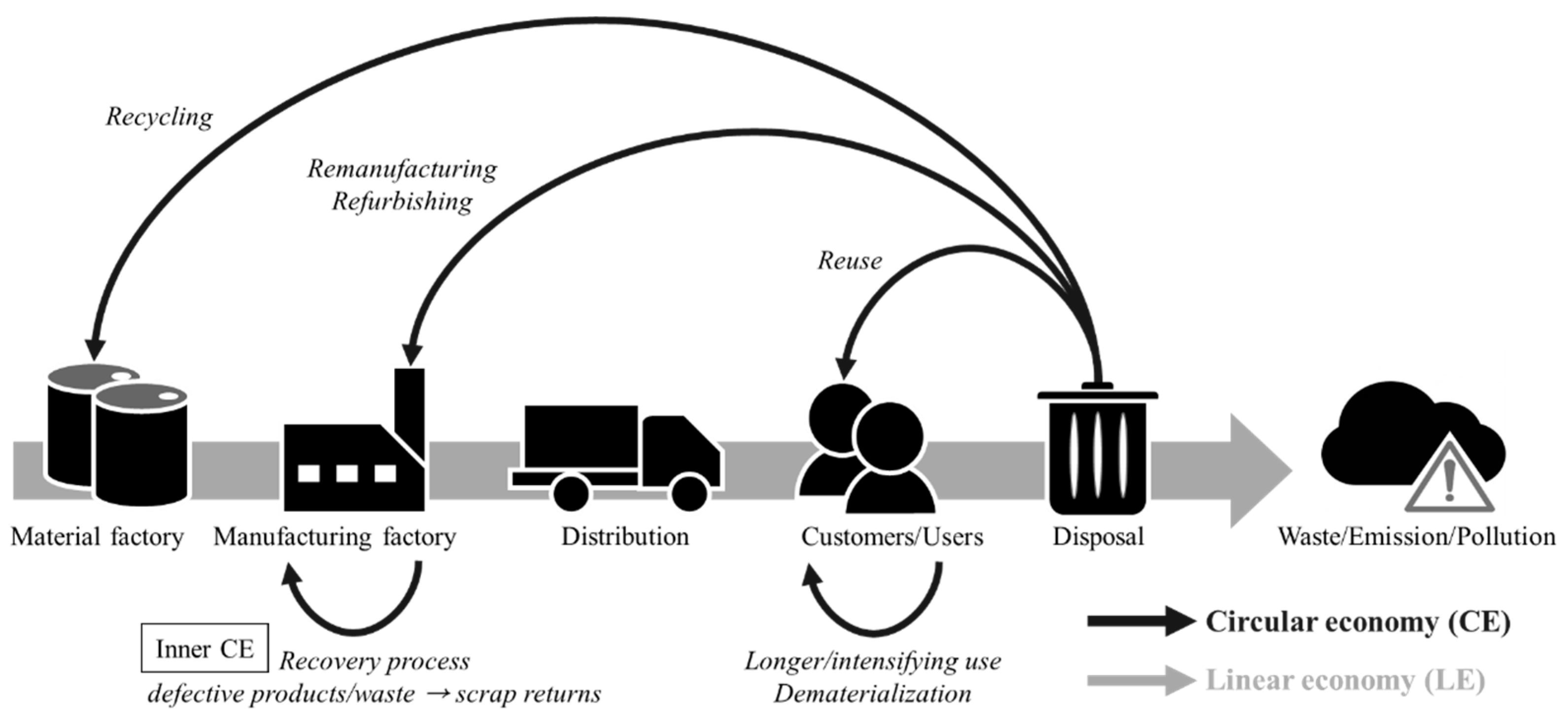
This can not only control costs to improve financial performance of enterprises by reducing waste, but also is one of implements of the circular economy (CE), which is particularly evident in industries with GM. CE is an economic system aimed at eliminating waste and the continual use of resources. Circular systems employ reuse, sharing, repair, refurbishment, remanufacturing, and recycling to create a closed-loop system, minimizing the use of resource inputs and the creation of waste, pollution, and carbon emissions [33]. Waste materials and energy should become inputs for other processes: either a component or recovered resource for another industrial process or as regenerative resources for nature. This regenerative approach is in contrast to the traditional linear economy (LE), which has a “take, make, dispose” model of production [34]. According to Geissdoerfer et al. [35], the latest schematic diagram for comparison of LE and CE is constructed in Figure 1. From Figure 1, it is shown that the recovery process converting the defective products (or waste) to scrap returns is an inner CE in a manufacturing factory. It is also a kind of GM. It is noted that the aim of GM is to reduce natural resource use, pollution, and waste, recycle and reuse materials, and moderate emissions in processes. Nowadays, many GM industries that have implemented CE actions have obtained great results. For example, sulfuric acid is an important raw material in the semiconductor etching process. In recent years, semiconductor manufacturers have devoted themselves to invest in the purification technology of waste sulfuric acid in order to reduce the natural mining of sulfur. In metal and plastic products manufacturing industries, the defective products can be converted into secondary raw materials by the melting process. This gap in the research motivated us to study an inner CE model capable of accounting for another method of disposal for defective products when discussing the issue of the imperfect production–inventory problem.
To summarize the above motivations, this paper analyzes an imperfect production–inventory model with inner CE activity. The detailed descriptions of the proposed system are as follows: (1) a production–inventory model involving manufacturer, raw material supplier, and customer is established based on economic order quantity (EOQ) and EPQ models; (2) the imperfect process with the random state shift is considered; (3) the defective product cannot be reworked or sold with discounted price, but can be converted into scrap returns through specific equipment for self or other production line use; (4) the efficiency of converted equipment is also considered in this paper; and (5) the production system produces paired products made from mixed materials containing scrap returns. A mathematical analysis method is used to prove the existence and uniqueness of optimal solutions and an algorithm for finding the optimal solution is also developed. Further, a practical case of pulp and paper industry is presented and a numerical example with values that represent real-world situations is then adopted to verify the proposed model. Finally, we further implement the sensitivity analysis to explore trends in the optimal policies and obtain some interesting observations and managerial implications for the manufacturer or manager. The rest of this paper is organized as follows. Section 2 establishes the notation and assumptions used through the whole paper. Section 3 presents the mathematical formulations, theoretical results, and solution procedure for this inventory model. Section 4 introduces a real CE scenario in the pulp and paper industry to enhance the relevance of our model in the real world; the numerical examples from this CE case are presented to illustrate a solution procedure, and a sensitivity analysis based on this example is performed to provide some managerial insights and decision-making advice. Finally, Section 5 concludes this paper and gives some future research directions.
2. Notation and Assumptions
This paper formulates a production–inventory model for paired products in an imperfect production system with inner CE activity. For convenience, the notation including system parameters and decision variables are listed as follows:
| System parameters: | |
| set-up and ordering costs per cycle. | |
| feed rate of new material in production in units. | |
| feed rate of scrap returns for product in units, where . | |
| production rate of finished product in units. | |
| demand rate for product in units, where . | |
| defective rate of finished product at stage, where | |
| maximum inventory level of scrap returns. | |
| maximum inventory level for product , where . | |
| inventory level of scrap returns when the stage of in-control transfers to out-of-control. | |
| inventory level of finished product when the stage of in-control transfers to out-of-control. | |
| holding cost of scrap returns per unit per unit time. | |
| holding cost of new material per unit per unit time. | |
| holding cost for a product per unit time, where . | |
| production, labor and inspection costs for a finished product. | |
| production cost for returning a defective product to scrap returns. | |
| opportunity cost for a unreturnable defective product , where . | |
| purchasing cost of material per unit. | |
| time period prior to depletion of inventory for product , , where . | |
| time period during in-control state, . | |
| Decision variables: | |
| production run time of product , , where . | |
| order quantity of new material per cycle. | |
| recovery rate of scrap returns. | |
The model is developed based on the following assumptions:
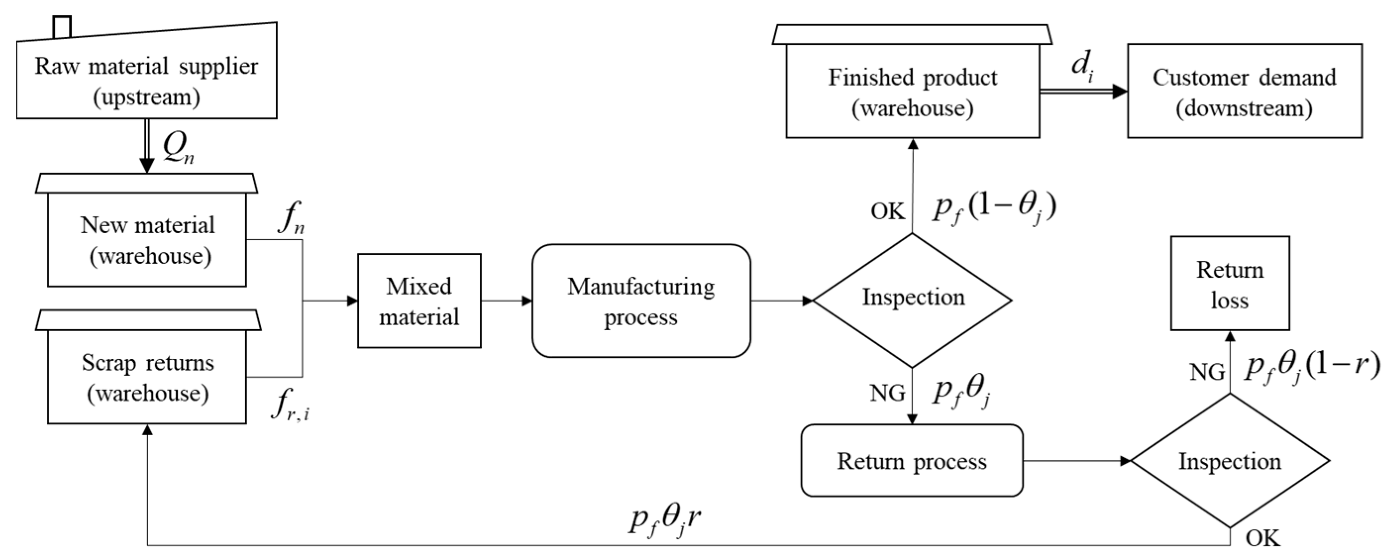
- The paired products with mixed materials containing scrap returns are considered in an imperfect production system. Figure 2 presents a schematic illustration of the proposed production system. From Figure 2, it can be seen that the processes and composition of mixed materials for two products are the same. Therefore, the production, labor, inspection, and material costs are also the same. The main material is ordered from a raw material supplier (upstream), and the order quantity is . The manufacturing process and return processes are both imperfect. Based on Rosenblatt and Lee [31], we assume that the manufacturing process may randomly shift from an in-control state to an out-of-control state, and the defective rate of finished product in the out-of-control state is higher than the in-control state, i.e., . The defective products from the manufacturing process forward to the return process, and the feed rate of defective product is , where . Only part of the defective products can be turned into scrap returns, and the production rate of scrap returns is , where . Note that the inspection time is so short that it can be disregarded.
- There are two products in the production system and the production sequence is product 1 to product 2. For product 1, the feed rate of scrap returns is less than or equal to the production rate of scrap returns to avoid the stage starves due to a lack of input from the previous stage, i.e., . For product 2, in order to avoid the unlimited accumulation of scrap returns, the feed rate of scrap returns must be higher than the production rate of scrap returns, i.e., . Based on the assumption , the following condition must be satisfied: . After rearranging the above inequality, it can be obtained that the reasonable range of recovery rate of scrap returns is . Note that the upper bound of must be less than or equal to 1, so which implies .
- The time period, , is a random variable that obeys a normal distribution with unknown mean and standard deviation . This paper adopts the lower confidence bound of mean to estimate the conservative value of by collecting the historical data.
- As far as we know, the production time of product 2 begins in the out-of-control period. The main reason is that the defective rate increases, and the feed rate of scrap returns must be faster to avoid the unlimited accumulation of scrap returns. Therefore, the production run time of product 1 must be higher than or equal to the length of time during the out-of-control period, i.e., .
- The recovery rate of scrap returns can be promoted through capital investment in return process improvement. Therefore, the capital investment can be treated as an increasing function of the recovery rate.
- Shortages are not allowed, and the following condition must be held: , where and .
3. Model Formulation
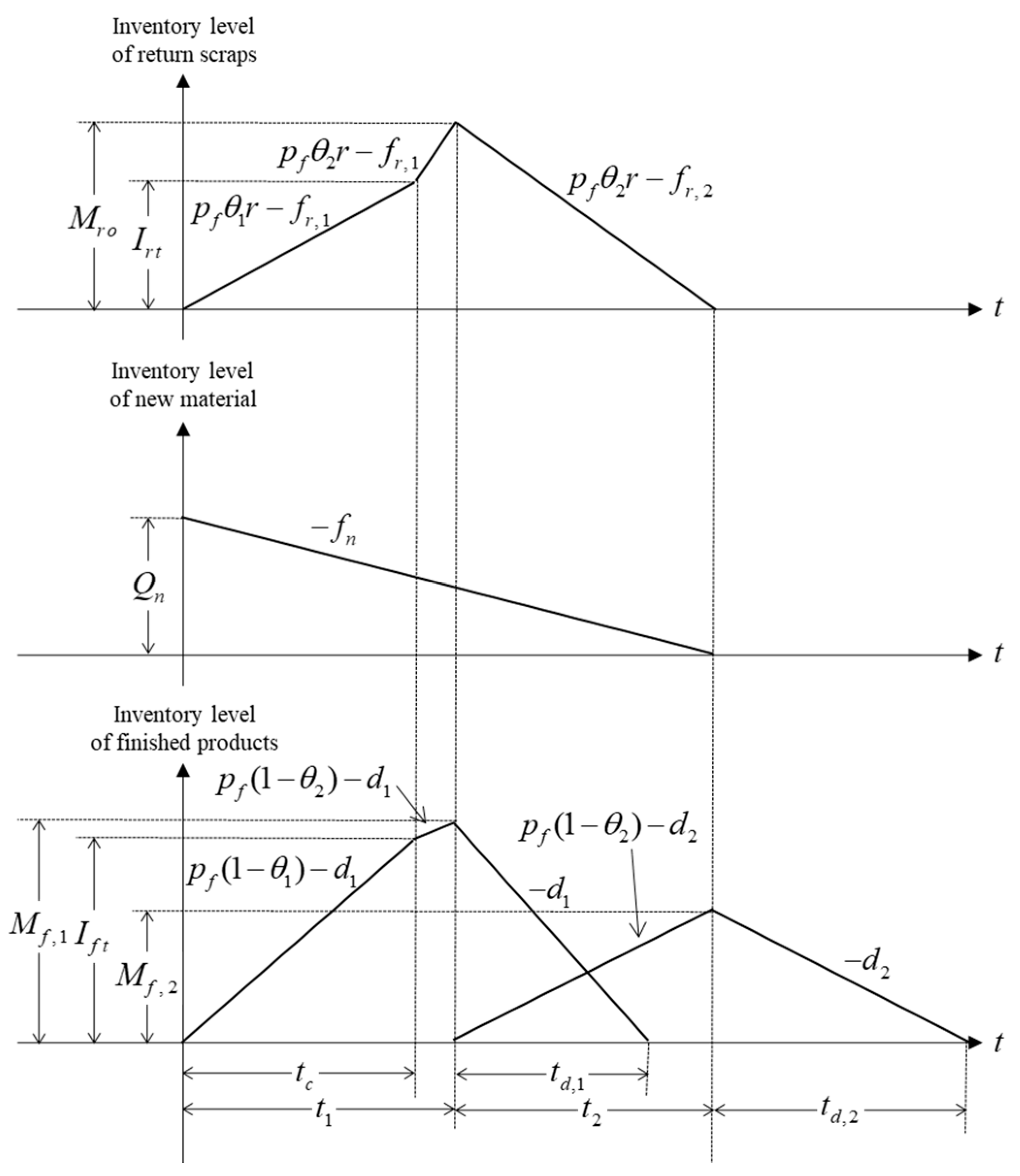
In this section, the mathematical model is developed based on the above assumptions. First, for the given time period , the inventory levels of scrap returns, new material, and finished products for an imperfect production system are depicted in Figure 3. Based on Figure 3, some relationships can be obtained as follows:
- R1.
- The maximum inventory level of scrap returns can be written asAfter rearranging the above equation, we obtain the following:
- R2.
- The maximum inventory level of the finished product 1 can be described as follows:After rearranging the above equation, we obtain the following:
- R3.
- The maximum inventory level of the finished product 2 can be described as follows:After rearranging the above equation, we obtain the following:
- R4.
- The ordering quantity of the material per cycle can also be described as the product of feed rate and total production time, i.e.,
In addition to considering some basic production and operation costs, we also further take into account all possible inventory costs, as well as the disposal, investment, and opportunity costs caused by imperfect production. Based on the above results, the elements of the total cost per cycle are established as follows:
- (a)
- Set-up and ordering costs (denoted by ): The set-up cost includes the costs associated with checking the initial output, adjusting the equipment, laying out the workplace, preparing the materials, preheating the boiler, etc. As to the ordering cost, it always includes delivery charges or the cost of labor required to place, receive, and stock an order. To facilitate the development of the model, set-up and ordering cost per cycle is treated as a fixed constant which implies .
- (b)
- Holding cost: From Figure 3, it is shown that this production system considers the stocks of scrap returns, new material, and two finished products. Each element of the holding cost per cycle is established as follows:
- (b-1)
- Holding cost of scrap returns (denoted by ):
- (b-2)
- Holding cost of new material (denoted by ):
- (b-3)
- Holding cost of finished product 1 (denoted by ):
- (b-4)
- Holding cost of finished product 2 (denoted by ):
- (c)
- Production cost (denoted by ): The production cost is the unit production cost for the finished product multiplied by the yield of the finished product, , which is:
- (d)
- Return cost for defective products (denoted by ): Due to the imperfect production system, defective products with units will be returned. As the unit cost per returned defective product is , the return cost for defective products per cycle is:
- (e)
- Opportunity cost due to lost return (denoted by ): This cost is the unit lost cost for the unreturnable defective product multiplied by the yield of the unreturnable defective product. The unreturnable volumes of products 1 and 2 per cycle are and , respectively. After multiplying the respective costs, the opportunity cost per cycle is:
- (f)
- Investment in converted equipment (denoted by ): The investment cost is an increasing function of recovery rate. In this paper, we consider an exponential form of investment function, which is:where denotes the percentage increase in per dollar increase in and is the original recovery rate of scrap returns.
- (g)
- Purchasing cost of material (denoted by ): This cost is the unit purchasing cost multiplied by the ordering quantity of material, which is:
To summarize the above results, the total cost per unit time (denoted by ) can be obtained as follows:
where , , , and .
The purpose of this paper is to determine the optimal lengths of production and recovery rate such that the total cost per unit time is minimal. From Equation (1), it is known that , shown in Equation (5), can be reduced to . Hence, the objective of this paper is only to find the optimal values of and with the aim of minimizing total cost per unit time. In order to verify the convexity of with respect to and , we need the following lemmas.
Lemma 1.
,, andincrease linearly when.
Proof of Lemma 1.
Based on Equations (1)–(3), taking the first and second derivatives of , and with respect to , we get:
Therefore, it is obvious that , , and increase linearly when . This completes the proof. □
Lemma 2.
andare increasing and convex in .
Proof of Lemma 2.
Based on Equations (1) and (3), taking the first and second derivatives of , and with respect to , we get:
. Therefore, it is obvious that , and are increasing and convex in . This completes the proof. □
We then apply the theoretical results in the pseudo-convex fractional function to prove that the optimal value not only exist but is also unique. The real-value function is pseudo-convex, if is non-negative, differentiable, and strictly convex, and is positive and affine (please refer to Cambini and Martein [36]). Based on the abovementioned theoretical results, we have the following theorems:
Theorem 1.
For given, the total cost per unit timeis pseudo-convex function inand there exists a unique minimum solution.
Proof of Theorem 1.
From Equation (5), for any given , let
and
Based on Lemma 1, taking the first-order and second-order derivatives of with respect to , we get:
and
From the above results, is non-negative, differentiable, and strictly convex. Therefore, for given , the total cost per unit time is pseudo-convex function in and there exists a unique minimum solution. This completes the proof. □
Theorem 2.
For given, the total cost per unit timeis pseudo-convex function inand there exists a unique minimum solution.
Proof of Theorem 2.
From Equation (5), for any given , define and as the functions of and equal to the right-hand side of Equations (6) and (7), respectively. Based on Lemma 2, taking the first-order and second-order derivatives of with respect to , we get:
and
From the above results, is non-negative, differentiable, and strictly convex. Therefore, for given , the total cost per unit time is a pseudo-convex function of and there exists a unique minimum solution. This completes the proof. □
Following this, to obtain the optimal solution , our method is to compare the minimun total cost per unit time under various values of , i.e., , and then find the optimal solution such that is minimum. The proposed method can ensure that the optimal solution meets assumptions (2) and (4). First, we calculate the first-order derivative of the total cost per unit time for a given value of with respect to i.e., . It is well known that the necessary condition for the optimal value of must satisfy the equation , then we get:
For convenience, we summarize the above results to build the following simple Algorithm 1 for finding the optimal solution :
| Algorithm 1 |
|
4. Application Example
In this section, we provide a case study involving a pulp and paper industry in Taiwan to present the practicality of our model. The procedure of the production system for this case is briefly introduced first. Then, a numerical example of this case is used to verify our analytical results. Based on the provided numerical example, we further implement the sensitivity analysis to explore trends in the optimal policies in order to obtain some interesting observations for the manufacturer or manager.
4.1. Pulp and Paper Industry
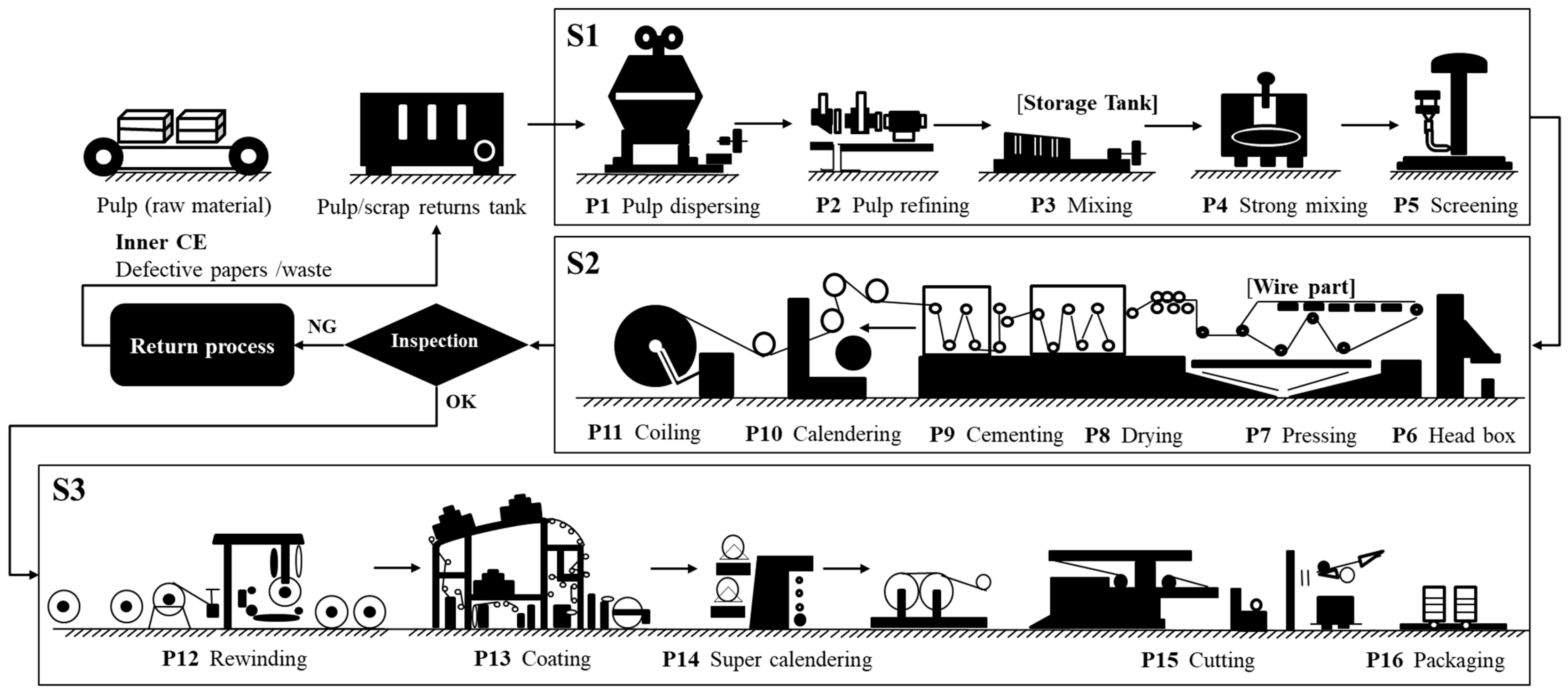
In the following, a well-established paper manufacturing firm in Taiwan is considered. The firm owns advanced machinery for papermaking, including a magazine grinder, a density controller, a pulp filtration machine, a headbox, press rolls, drying cylinders, gluing machines, calendaring machines, reeling machines, coating machines, chopping machines, and packaging machines. The company’s major business scope includes the medical, industrial, food, living, building materials, and garment industries. Based on [37], Figure 4 shows the process of manufacturing specific papers with inner CE activity. It is easy to see that the process includes three major stages, preparation of papermaking material (S1), paper production (S2), and paper processing (S3). At stage S1, the primary material of paper is pulp made from hardwood trees and softwood trees (called virgin wood fibers) and recycled paper (called recycled wood fibers). Since the pulp manufacturing in this firm is not the main business, the manufacturer usually orders it from a pulp manufacturing factory (upstream). However, the ordered pulp cannot be used directly, it must pass five processing stations (P1–P5) to become the raw material for paper production. After passing P6–P11 at stage S2, the raw material becomes pure paper in roll form. At this stage, the production system is imperfect, and it makes some defective paper or waste due to the deterioration of appliances. Some particular papers can implement inner CE activity, that is, the defective papers and waste can be converted into the scrap returns (secondary raw material) through specific processing in converted equipment. Finally, according to the specifications and requirements of the order, the customized papers are manufactured at stage S3. In an effort to optimize the overall inputs/outputs, the firm usually decides the optimal production run time, the investment in converted equipment, and ordering quantity of pulp before starting production.
4.2. Numerical Example
By conducting surveys and interviews with relevant staff at this company, we decided on some base settings for the system parameters for our model. Note that the values of parameters have been altered to preserve the confidentiality of this commercial information. The values of system parameters are listed as follows:
- i.
- Demand of two products: 400 kg/day and 300 kg/day.
- ii.
- Operation for production and purchasing: $10,000/cycle, $10/kg, 600 kg/day, $5/kg, 100 kg/day, 2 kg/day and 40 kg/day.
- iii.
- Operation for stock: $0.6/kg/day, $0.4/kg/day $0.3/kg/day and $0.2/kg/day.
- iv.
- Defective rate of finished product: and .
- v.
- Operation for recovery activity: $2/kg, $0.15/kg, $0.1/kg, and .
- vi.
- Algorithm parameter: .
- vii.
- Time length of in-control period (): This paper considers a conservative estimate to express the value of due to the uncertainty of the time length of the in-control period. Assuming that the time length obeys a normal distribution, we use the lower confidence bound of time length (denoted by ) to express the conservative estimate under the confidence level, i.e.,where and for the given sample ; is quantile of Student’s T distribution with degrees of freedom. Table 2 presents historical data (28 cycles) of time length of in-control period (measured in days). First, we perform Anderson–Darling and Shapiro–Wilk normality tests with R software. The p-values in the two tests both exceed 0.1, i.e., there is no significant violation of the normal distribution. From Table 2, we calculate the sample mean 3.4979 days, sample standard deviation 0.0556 days and 3.4799 days with 95% confidence level, then let 3.4799 days.
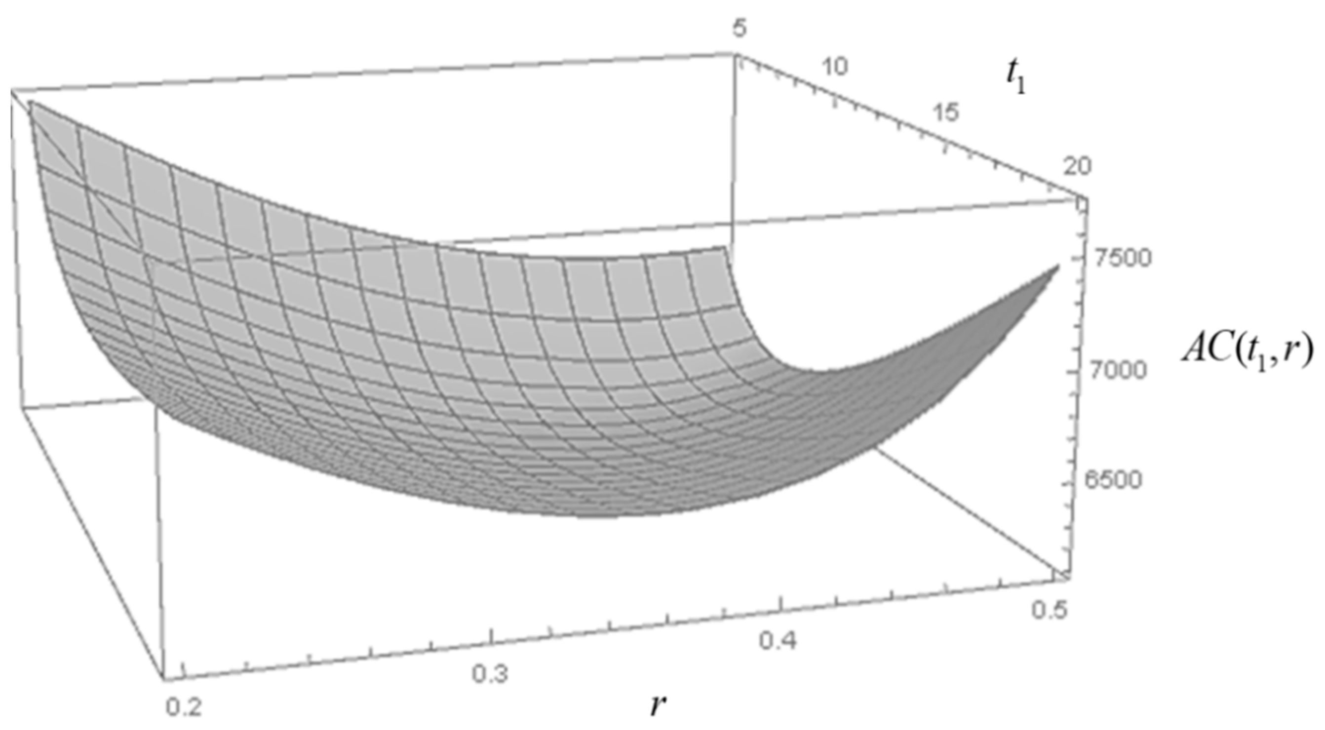
By applying the proposed algorithm, we can obtain the optimal solutions, 9.6587 days, 12.4212 days, 0.42295, 2207.99 kg, and $6096.79. The three-dimensional total cost per unit time is shown in Figure 5. From Figure 5, the convexity of the total cost per unit time can be verified, and the obtained solutions are optimal for minimizing the total cost per unit time. Regarding the results of the CE activity, we can multiply the production rate of scrap returns by the production time to get the total production volume of secondary materials, i.e., 484.7007 kg. Note that the production volume of secondary materials can also express the recycling capacity of resources in this case.
4.3. Sensitivity Analysis
Based on the presented numerical example in Section 4.2, we further study the sensitivity analysis that discusses the effects of changes to system parameters (, , , , , , , , , , , and ) on the values of , , , , and . Each parameter is adjusted separately (i.e., the others parameters are kept unchanged) by +50%, +25%, −25%, or −50%. The results of the sensitivity analysis are presented in Table 3. According to the data trend in Table 3, we find some interesting observations, which could be referred to as guide for decision-making:
- M1.
- Increasing the cost parameters (, , , , , , , , or ) or decreasing the defective rate of finished product ( or ) would lead to an increase in the total cost per unit time. Moreover, the total cost per unit time is relatively sensitive to the product cost, the defective rate of finished product at out-of-control stage, and the holding cost of product 2. From the perspective of business operations, if companies want to effectively reduce total cost per unit time, they can start from these relatively high-sensitivity parameters.
- M2.
- In terms of holding cost parameters , , , and , increasing the values of the parameters led to corresponding decreases in , and except that an increase in causes increases in . It implies that the managers should shorten the length of the production cycle as holding costs increase. As to the exception of the impact of change on , the reason is the production sequence is product 1 to product 2 in the proposed model. When the value of increases, the manufacturer will shorten the length of the production cycle for product 1 and start producing product 2 ahead of schedule, resulting in an increase in the length of production cycle for product 2.
- M3.
- As the set-up and ordering cost increases, the values of , , , and increase. It’s intuitive that the quantity of materials ordered and the recovery rate of scrap returns each time will increase and that the length of the production cycle will be extended when the fixed cost increases.
- M4.
- With the increase in the value of cost parameter , , or , the optimal value of decreases while the optimal values of , , and increase.
- M5.
- All the optimal values of , , , and decrease as the value of or increases. This implies that the higher the oportunity cost for unreturnable defective product 2 or the defective rate of finished product at in-control stage, the shorter the length of production cycle and the lower recovery rate of scrap returns and the order quantity of material will be.
- M6.
- When the defective rate of finished product at out-of-control stage inceases, the value of will decrease at an increasing rate but the value of will increase at a decreasing rate such that the value of increases first and then decreases. Moreover, the recovery rate of scrap returns will be reduced when the defective rate of finished product at the out-of-control stage increases.
- M7.
- As the value of reproduction cost increases , the optimal values of and decrease but the optimal values of and increase. This implies that the defective products should be converted to scrap returns as much as possible for recycling due to high return costs. Note that the effect of this parameter change on the optimal solutions is the same as that of the holding cost .
- M8.
- For the investment in converted equipment, and decrease but , , and increase when the value of increases. It implies that the cost-effectiveness of the investment is worse with higher values of percentage increase in investment capital to improve the recovery rate of scrap returns.
5. Conclusions
The proposed model explored the practicality of a production–inventory model with paired products mixed materials containing scrap returns in an imperfect production system. It aimed to clearly determine the production run time of both finished products, order quantity of material, and the investment capital in converted equipment to minimize the total cost per unit time. Several theoretical results were developed to verify the convexity of the optimal solutions of the model and an algorithm to find the optimal solution was also provided. Further, we took a pulp and paper manufacturing firm in Taiwan as an example to perform a numerical analysis to verify the model and conducted a sensitivity analysis to obtain managerial insights. For instance, the amount of scrap can be reduced more for the CE investment in converted equipment in order to avoid serious waste of natural resources. In this case, 484.7007 kg material per cycle can be saved. However, the cost-effectiveness of the investment is worse with a higher percentage increase in investment capital to improve the recovery rate of scrap returns. In addition, improving production cost can effectively reduce the total cost per unit time, for example, a 34.6177% reduction in the total cost can be achieved if the unit production cost of the finished product is reduced by half. Regarding the improvement in the stock environment, one can focus on the preservation of product 2 because the change in its holding cost has the highest sensitivity to the total cost per unit time. Additionally, as to the impact of the defective rate on the recovery rate of scrap returns, the results show that the recovery rate of scrap returns should be reduced as the defective rate of finished product at the in-control stage increases while the defective rate of finished product at the out-of-control stage also increases. Based on the above, it is our belief that the results of this study should serve as a useful reference for decision makers in practical applications.
Regarding future research, there are some critical issues worthy of study. For example, it may focus on evaluating the deterioration of items, including raw materials and finished products. Additionally, the proposed model can also be extended by incorporating a pricing strategy, a variable demand rate, or allowing for shortages, trade credit, etc.
Author Contributions
Conceptualization, methodology, formal analysis, writing—original draft preparation, R.-H.S. and C.-T.Y.; formal analysis, writing—review and editing, M.-W.W.; software, H.-T.L. All authors have read and agreed to the published version of the manuscript.
Funding
This work is partially supported by the Ministry of Science and Technology, Taiwan, under grant numbers MOST 110-2410-H-030-020 and MOST 110-2410-H-231-001-MY2.
Institutional Review Board Statement
Not applicable.
Informed Consent Statement
Not applicable.
Data Availability Statement
Not applicable.
Acknowledgments
The authors would like to thank the editor and anonymous reviewers for their valuable and constructive comments, which have led to a significant improvement in the manuscript.
Conflicts of Interest
The authors declare no conflict of interest.
References
- Taft, E.W. The Most Economical Production Lot. Iron Age 1918, 101, 1410–1412. [Google Scholar]
- Darwish, M.; Ben-Daya, M. Effect of Inspection Errors and Preventive Maintenance on a Two-Stage Production Inventory system. Int. J. Prod. Econ. 2007, 107, 301–313. [Google Scholar] [CrossRef]
- Lee, H.-H. The Investment Model in Preventive Maintenance in Multi-Level Production Systems. Int. J. Prod. Econ. 2008, 112, 816–828. [Google Scholar] [CrossRef]
- Pearn, W.L.; Su, R.H.; Weng, M.W.; Hsu, C.H. Optimal Production Run Time for Two-Stage Production System with Imperfect Processes and Allowable Shortages. Central Eur. J. Oper. Res. 2010, 19, 533–545. [Google Scholar] [CrossRef]
- Sarker, B.R.; Jamal, A.; Mondal, S. Optimal Batch Sizing in a Multi-Stage Production System with Rework Consideration. Eur. J. Oper. Res. 2008, 184, 915–929. [Google Scholar] [CrossRef]
- Cárdenas-Barrón, L.E. On Optimal Batch Sizing in a Multi-Stage Production System with Rework Consideration. Eur. J. Oper. Res. 2009, 196, 1238–1244. [Google Scholar] [CrossRef]
- Chang, H.-J.; Su, R.-H.; Yang, C.-T.; Weng, M.-W. An economic Manufacturing Quantity Model for a Two-Stage Assembly System with Imperfect Processes and Variable Production Rate. Comput. Ind. Eng. 2012, 63, 285–293. [Google Scholar] [CrossRef]
- Sarkar, S.; Shewchuk, J.P. Use of Advance Demand Information in Multi-Stage Production-Inventory Systems with Multiple Demand Classes. Int. J. Prod. Res. 2013, 51, 57–68. [Google Scholar] [CrossRef]
- Paul, S.K.; Sarker, R.; Essam, D. A Disruption Recovery Plan in a Three-Stage Production-Inventory System. Comput. Oper. Res. 2015, 57, 60–72. [Google Scholar] [CrossRef]
- Wang, Z.; Chan, F.T.S.; Li, M. A Robust Production Control Policy for Hedging Against Inventory Inaccuracy in a Multiple-Stage Production System with Time Delay. IEEE Trans. Eng. Manag. 2018, 65, 474–486. [Google Scholar] [CrossRef]
- Su, R.-H.; Weng, M.-W.; Huang, Y.-F. Innovative Maintenance Problem in a Two-Stage Production-Inventory System with Imperfect Processes. Ann. Oper. Res. 2019, 287, 379–401. [Google Scholar] [CrossRef]
- Su, R.-H.; Weng, M.-W.; Yang, C.-T. Effects of Corporate Social Responsibility Activities in a Two-Stage Assembly Production System with Multiple Components and Imperfect Processes. Eur. J. Oper. Res. 2020, 293, 469–480. [Google Scholar] [CrossRef]
- Chiu, Y.-S.P.; Huang, C.-C.; Wu, M.-F.; Chang, H.-H. Joint Determination of Rotation Cycle Time and Number of Shipments for a Multi-Item EPQ Model with Random Defective Rate. Econ. Model. 2013, 35, 112–117. [Google Scholar] [CrossRef]
- Sarkar, B.; Cárdenas-Barrón, L.E.; Sarkar, M.; Singgih, M.L. An Economic Production Quantity Model with Random Defective Rate, Rework Process and Backorders for a Single Stage Production System. J. Manuf. Syst. 2014, 33, 423–435. [Google Scholar] [CrossRef]
- Tayyab, M.; Sarkar, B. Optimal Batch Quantity in a Cleaner Multi-Stage Lean Production System with Random Defective Rate. J. Clean. Prod. 2016, 139, 922–934. [Google Scholar] [CrossRef]
- Kang, C.W.; Ullah, M.; Sarkar, B.; Hussain, I.; Akhtar, R. Impact of Random Defective Rate on Lot Size Focusing Work-In-Process Inventory in Manufacturing System. Int. J. Prod. Res. 2017, 55, 1748–1766. [Google Scholar] [CrossRef]
- Sarkar, B.; Dey, B.K.; Pareek, S.; Sarkar, M. A Single-Stage Cleaner Production System with Random Defective Rate and Remanufacturing. Comput. Ind. Eng. 2020, 150, 106861. [Google Scholar] [CrossRef]
- Chung, C.-J.; Widyadana, G.A.; Wee, H.M. Economic Production Quantity Model for Deteriorating Inventory with Random Machine Unavailability and Shortage. Int. J. Prod. Res. 2011, 49, 883–902. [Google Scholar] [CrossRef]
- Widyadana, G.A.; Wee, H.M. Optimal Deteriorating Items Production Inventory Models with Random Machine Breakdown and Stochastic Repair Time. Appl. Math. Model. 2011, 35, 3495–3508. [Google Scholar] [CrossRef]
- Öztürk, H. Modeling an Inventory Problem with Random Supply, Inspection and Machine Breakdown. Opsearch 2019, 56, 497–527. [Google Scholar] [CrossRef]
- Öztürk, H. Optimal Production Run Time for an Imperfect Production Inventory System with rework, Random Breakdowns and Inspection Costs. Oper. Res. 2021, 21, 167–204. [Google Scholar] [CrossRef]
- Pal, B.; Adhikari, S. Random Machine Breakdown and Stochastic Corrective Maintenance Period on an Economic Production Inventory Model with Buffer Machine and Safe Period. RAIRO Oper. Res. 2021, 55, S1129–S1149. [Google Scholar] [CrossRef]
- Chiu, Y.-S.P.; Wu, C.-S.; Wu, H.Y.; Chiu, S.W. Studying the Effect of Stochastic Breakdowns, Overtime, and Rework on Inventory Replenishment Decision. Alex. Eng. J. 2021, 60, 1627–1637. [Google Scholar] [CrossRef]
- Sarkar, B. An Inventory Model with Reliability in an Imperfect Production Process. Appl. Math. Comput. 2012, 218, 4881–4891. [Google Scholar] [CrossRef]
- Li, N.; Chan, F.T.S.; Chung, S.H.; Tai, A.H. A Stochastic Production-Inventory Model in a Two-State Production System with Inventory Deterioration, Rework Process, and Backordering. IEEE Trans. Syst. Man Cybern. Syst. 2016, 47, 916–926. [Google Scholar] [CrossRef]
- Mahata, G.C. A Production-Inventory Model with Imperfect Production Process and Partial Backlogging under Learning Considerations in Fuzzy Random Environments. J. Intell. Manuf. 2014, 28, 883–897. [Google Scholar] [CrossRef]
- Huang, H.; He, Y.; Li, D. Coordination of Pricing, Inventory, and Production Reliability Decisions in Deteriorating Product Supply Chains. Int. J. Prod. Res. 2018, 56, 6201–6224. [Google Scholar] [CrossRef]
- Dey, B.K.; Sarkar, B.; Sarkar, M.; Pareek, S. An Integrated Inventory Model Involving Discrete Setup Cost Reduction, Variable Safety Factor, Selling Price Dependent Demand, and Investment. RAIRO Oper. Res. 2019, 53, 39–57. [Google Scholar] [CrossRef] [Green Version]
- Manna, A.K.; Das, B.; Tiwari, S. Impact of Carbon Emission on Imperfect Production Inventory System with Advance Payment Base Free Transportation. RAIRO Oper. Res. 2020, 54, 1103–1117. [Google Scholar] [CrossRef]
- Dey, B.K.; Pareek, S.; Tayyab, M.; Sarkar, B. Autonomation Policy to Control Work-in-Process Inventory in a Smart Production System. Int. J. Prod. Res. 2021, 59, 1258–1280. [Google Scholar] [CrossRef]
- Rosenblatt, M.J.; Lee, H.L. Economic Production Cycles with Imperfect Production Processes. IIE Trans. 1986, 18, 48–55. [Google Scholar] [CrossRef]
- Love, P. Influence of Project Type and Procurement Method on Rework Costs in Building Construction Projects. J. Constr. Eng. Manag. 2002, 128, 18–29. [Google Scholar] [CrossRef] [Green Version]
- Geissdoerfer, M.; Savaget, P.; Bocken, N.M.P.; Hultink, E.J. The Circular Economy—A new sustainability paradigm? J. Clean. Prod. 2017, 143, 757–768. [Google Scholar] [CrossRef] [Green Version]
- MacArthur, E. Towards the Circular Economy, Economic and Business Rationale for an Accelerated Transition; Ellen MacArthur Foundation: Cowes, UK, 2013; pp. 21–34. [Google Scholar]
- Geissdoerfer, M.; Pieroni, M.P.; Pigosso, D.C.; Soufani, K. Circular Business Models: A review. J. Clean. Prod. 2020, 277, 123741. [Google Scholar] [CrossRef]
- Cambini, A.; Martein, L. Generalized Convexity and Optimization. Mult. Criteria Decis. Mak. 2009, 616. [Google Scholar] [CrossRef]
- How do we Make Pulp and Paper? Available online: http://www.chp.com.tw/en/product/product_learn (accessed on 16 July 2021).
Figure 1.
A brief introduction to CE and LE.

Figure 2.
Proposed imperfect production system with scrap recovery activities.

Figure 3.
Graph of inventory levels for scrap returns, material, and finished product.

Figure 4.
Production system for the manufacturing process of paper with inner CE.

Figure 5.
Graphical illustration of the total cost per unit time with and .


Table 1.
A brief comparison of imperfect production systems by year.
| Literatures | Stage | Imperfect Process | Disposal Ways | |||||
|---|---|---|---|---|---|---|---|---|
| CD | RD | RB | RS | RW | SP | PD | ||
| Darwish and Ben-Daya [2] | MS | V | V | |||||
| Lee [3] | MS | V | V | |||||
| Sarker et al. [5] | MS | V | V | |||||
| Cárdenas-Barrón [6] | MS | V | V | |||||
| Pearn et al. [4] | MS | V | V | |||||
| Chung et al. [18] | SS | V | V | |||||
| Widyadana and Wee [19] | SS | V | V | |||||
| Chang et al. [7] | MS | V | V | |||||
| Sarkar [24] | SS | V | V | |||||
| Sarkar and Shewchuk [8] | MS | |||||||
| Chiu et al. [13] | SS | V | V | |||||
| Sarkar et al. [14] | SS | V | V | |||||
| Paul et al. [9] | MS | |||||||
| Tayyab and Sarkar [15] | MS | V | V | |||||
| Kang et al. [16] | SS | V | V | V | ||||
| Li et al. [25] | SS | V | V | V | ||||
| Mahata [26] | SS | V | V | |||||
| Wang et al. [10] | MS | V | ||||||
| Huang et al. [27] | SS | V | V | |||||
| Öztürk [20] | SS | V | V | V | ||||
| Dey et al. [28] | SS | V | V | |||||
| Su et al. [11] | MS | V | V | |||||
| Sarkar et al. [17] | SS | V | V | |||||
| Manna et al. [29] | SS | V | V | V | ||||
| Su et al. [12] | MS | V | V | |||||
| Öztürk [21] | SS | V | V | V | ||||
| Pal and Adhikari [22] | SS | V | ||||||
| Chiu et al. [23] | SS | V | V | |||||
| Dey et al. [30] | SS | V | V | |||||
Note: single stage (SS), multiple stage (MS), constant defective rate (CD), random defective rate (RD), random machine breakdowns (RB), random state shift (RS), rework process (RW), repair process (RP), scrap process (SP), price discount (PD).
Table 2.
28 sample data of time length of in-control period.
| 3.57 | 3.60 | 3.58 | 3.48 | 3.49 | 3.54 | 3.43 |
| 3.55 | 3.54 | 3.48 | 3.50 | 3.51 | 3.52 | 3.41 |
| 3.43 | 3.49 | 3.41 | 3.43 | 3.54 | 3.48 | 3.50 |
| 3.56 | 3.54 | 3.41 | 3.52 | 3.41 | 3.52 | 3.50 |
Table 3.
Effect of changes in various parameters based on numerical example.
| Parameters | % Change | % Change in | ||||
|---|---|---|---|---|---|---|
| −50 | −7.3178 | −15.5275 | −2.6008 | −11.9357 | −2.7382 | |
| −25 | −3.4228 | −7.3825 | −1.1727 | −5.6504 | −1.3214 | |
| 25 | 3.0781 | 6.8053 | 0.9930 | 5.1744 | 1.2452 | |
| 50 | 5.8900 | 13.1525 | 1.8513 | 9.9756 | 2.4275 | |
| −50 | 0.0186 | −0.0403 | −0.0236 | −0.0145 | −0.0105 | |
| −25 | 0.0093 | −0.0201 | −0.0118 | −0.0072 | −0.0052 | |
| 25 | −0.0093 | 0.0209 | 0.0118 | 0.0072 | 0.0052 | |
| 50 | −0.0197 | 0.0411 | 0.0236 | 0.0145 | 0.0105 | |
| −50 | 0.0021 | 0.0040 | 0.0007 | 0.0032 | −0.0110 | |
| −25 | 0.0010 | 0.0024 | 0.0002 | 0.0014 | −0.0056 | |
| 25 | −0.0010 | −0.0016 | −0.0002 | −0.0014 | 0.0056 | |
| 50 | −0.0021 | −0.0032 | −0.0005 | −0.0027 | 0.0110 | |
| −50 | 4.3815 | −22.7868 | −11.2685 | −10.9027 | −34.6177 | |
| −25 | 2.1970 | −11.0931 | −5.1614 | −5.2795 | −17.1267 | |
| 25 | −2.2343 | 10.6093 | 4.4686 | 4.9910 | 16.8248 | |
| 50 | −4.5141 | 20.8136 | 8.4100 | 9.7346 | 33.3928 | |
| −50 | 0.3686 | −1.8122 | −0.8062 | −0.8587 | −2.8321 | |
| −25 | 0.1843 | −0.9041 | −0.4019 | −0.4280 | −1.4150 | |
| 25 | −0.1843 | 0.9017 | 0.3972 | 0.4262 | 1.4129 | |
| 50 | −0.3696 | 1.7993 | 0.7873 | 0.8505 | 2.8238 | |
| −50 | 0.2247 | −0.1385 | −0.1466 | 0.0204 | −0.6254 | |
| −25 | 0.1118 | −0.0692 | −0.0733 | 0.0100 | −0.3126 | |
| 25 | −0.1118 | 0.0692 | 0.0733 | −0.0100 | 0.3126 | |
| 50 | −0.2226 | 0.1377 | 0.1466 | −0.0199 | 0.6251 | |
| −50 | 6.5226 | −1.8340 | −3.4307 | 1.8216 | −1.6250 | |
| −25 | 2.9621 | −0.9524 | −1.6172 | 0.7600 | −0.7896 | |
| 25 | −2.5262 | 1.0104 | 1.4683 | −0.5362 | 0.7507 | |
| 50 | −4.7201 | 2.0698 | 2.8207 | −0.9004 | 1.4678 | |
| −50 | 8.8097 | 46.3055 | 9.3912 | 29.9032 | −4.2432 | |
| −25 | 3.7842 | 17.5659 | 4.0218 | 11.5372 | −1.8803 | |
| 25 | −2.9642 | −12.0721 | −3.2368 | −8.0874 | 1.5741 | |
| 50 | −5.3589 | −20.9859 | −5.9558 | −14.1500 | 2.9340 | |
| −50 | 5.7948 | 8.7399 | 0.5012 | 7.4516 | −1.9371 | |
| −25 | 2.7447 | 4.1614 | 0.2530 | 3.5417 | −0.9520 | |
| 25 | −2.4879 | −3.8032 | −0.2601 | −3.2278 | 0.9221 | |
| 50 | −4.7594 | −7.2956 | −0.5202 | −6.1857 | 1.8169 | |
| −50 | 0.3417 | 0.3921 | −0.0118 | 0.3700 | −0.0960 | |
| −25 | 0.1698 | 0.1956 | −0.0047 | 0.1843 | −0.0479 | |
| 25 | −0.1688 | −0.1940 | 0.0047 | −0.1834 | 0.0479 | |
| 50 | −0.3365 | −0.3880 | 0.0118 | −0.3655 | 0.0955 | |
| −50 | −21.1830 | 3.0738 | 11.2685 | −7.5372 | −3.9855 | |
| −25 | −9.1110 | 1.4870 | 4.6672 | −3.1490 | −1.7307 | |
| 25 | 7.3654 | −1.4008 | −3.6198 | 2.4343 | 1.4229 | |
| 50 | 13.5639 | −2.7292 | −6.5800 | 4.3981 | 2.6404 | |
| −50 | 9.7197 | 4.0157 | 1.3997 | 6.5109 | 1.2767 | |
| −25 | 4.8619 | 1.9974 | 0.7046 | 3.2505 | 0.6382 | |
| 25 | −4.8650 | −1.9748 | −0.7164 | −3.2391 | −0.6380 | |
| 50 | −9.7322 | −3.9255 | −1.4399 | −6.4656 | −1.2756 | |
| −50 | 35.6414 | −62.0053 | −4.9249 | −19.2904 | 16.2904 | |
| −25 | 29.2203 | −25.2818 | 1.0427 | −1.4402 | 6.3468 | |
| 25 | −29.7752 | 14.7643 | −2.8845 | −4.7197 | −3.7374 | |
| 50 | −55.0478 | 24.5250 | −5.7619 | −10.2836 | −5.8816 | |
Publisher’s Note: MDPI stays neutral with regard to jurisdictional claims in published maps and institutional affiliations. |
© 2021 by the authors. Licensee MDPI, Basel, Switzerland. This article is an open access article distributed under the terms and conditions of the Creative Commons Attribution (CC BY) license (https://creativecommons.org/licenses/by/4.0/).
Share and Cite
MDPI and ACS Style
Su, R.-H.; Weng, M.-W.; Yang, C.-T.; Li, H.-T. An Imperfect Production–Inventory Model with Mixed Materials Containing Scrap Returns Based on a Circular Economy. Processes 2021, 9, 1275. https://doi.org/10.3390/pr9081275
AMA Style
Su R-H, Weng M-W, Yang C-T, Li H-T. An Imperfect Production–Inventory Model with Mixed Materials Containing Scrap Returns Based on a Circular Economy. Processes. 2021; 9(8):1275. https://doi.org/10.3390/pr9081275
Chicago/Turabian StyleSu, Rung-Hung, Ming-Wei Weng, Chih-Te Yang, and Hsin-Ting Li. 2021. "An Imperfect Production–Inventory Model with Mixed Materials Containing Scrap Returns Based on a Circular Economy" Processes 9, no. 8: 1275. https://doi.org/10.3390/pr9081275
Note that from the first issue of 2016, this journal uses article numbers instead of page numbers. See further details here.