
Outlier Detection Based Feature Selection Exploiting Bio-Inspired Optimization Algorithms


Computer Science Department, College of Computer and Information Sciences, Prince Sultan University, P.O. Box 53073, Riyadh 11586, Saudi Arabia
Appl. Sci. 2021, 11(15), 6769; https://doi.org/10.3390/app11156769
Submission received: 25 June 2021
/
Revised: 15 July 2021
/
Accepted: 20 July 2021
/
Published: 23 July 2021
(This article belongs to the Special Issue Novel Research and Application on Swarm Optimization and Bioinspired Optimization Algorithms)
Abstract
:The curse of dimensionality problem occurs when the data are high-dimensional. It affects the learning process and reduces the accuracy. Feature selection is one of the dimensionality reduction approaches that mainly contribute to solving the curse of the dimensionality problem by selecting the relevant features. Irrelevant features are the dependent and redundant features that cause noise in the data and then reduce its quality. The main well-known feature-selection methods are wrapper and filter techniques. However, wrapper feature selection techniques are computationally expensive, whereas filter feature selection methods suffer from multicollinearity. In this research study, four new feature selection methods based on outlier detection using the Projection Pursuit method are proposed. Outlier detection involves identifying abnormal data (irrelevant features of the transpose matrix obtained from the original dataset matrix). The concept of outlier detection using projection pursuit has proved its efficiency in many applications but has not yet been used as a feature selection approach. To the author’s knowledge, this study is the first of its kind. Experimental results on nineteen real datasets using three classifiers (k-NN, SVM, and Random Forest) indicated that the suggested methods enhanced the classification accuracy rate by an average of 6.64% when compared to the classification accuracy without applying feature selection. It also outperformed the state-of-the-art methods on most of the used datasets with an improvement rate ranging between 0.76% and 30.64%. Statistical analysis showed that the results of the proposed methods are statistically significant.
1. Introduction
The data is continuously evolving, leading to a big challenge in several domains. It is generally high-dimensional, which causes the curse of the dimensionality problem. In this study, we investigated this problem with a high number of attributes (features). Reducing the space of features is performed through feature extraction or feature selection (FS). Feature extraction transforms the initial feature space into a novel low-dimensional feature space, for example, Kernel Dimensionality Reduction [1], Principal Component Analysis (PCA) [2], and Kernel PCA [3]. While FS does not produce new features but employs the original features to select the best ones, it consists of choosing a subgroup of significant features that mainly contribute to enhancing the output. FS is an essential preprocessing step in clustering and classification techniques to improve data quality. The effectiveness of FS method is one of the crucial aspects that affect the accuracy outcomes. The goal of the algorithm is to minimize the cardinality of the features set. Finding the most relevant features is not an easy task. For a dataset with a dimension d, there are potential subsets of features (excluding the empty subset) [4]. For even a reasonable value of d, it is of interest to choose a less computationally expensive method. FS is required in numerous domains and applications, for example, in bio-informatics [5,6], where the data can hold a large number of variables, most of wihich might be extremely well correlated with other variables. These variables are called dependent variables and do not deliver further information in the classification process, but they are considered as a noise for the classifier, which requires removing them to enhance the data quality. Another example in the biomedical domain wherein protein interaction discovery is vitally needed [7]. In biometric identification, FS is requested in facial recognition [8] to diminish the data dimensionality and then increase the classification accuracy. In addition, text mining suffers from the curse of dimensionality, and some FS methods were addressed in text categorization [9] and text clustering [10].
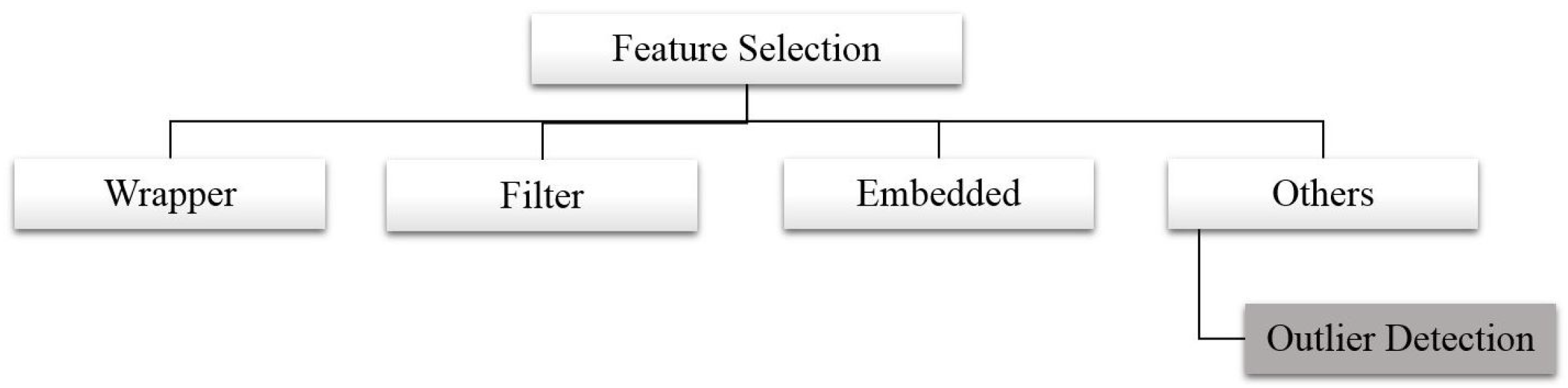
FS methods are classified into four categories, as displayed in Figure 1, called wrapper, filter, embedded, and outlier detection methods. Wrapper methods consist of evaluating features based on their predictive power using a classifier and usually a cross-validation technique. Several wrapper techniques have been proposed to solve the curse of dimensionality problem. They are based on a specific search method [11], such as the sequential selection [12], meta-heuristic (for example [13,14]), and local search [15]. The filter method is based on evaluating features using a criterion function that is relatively independent of classification such as distance [16], information [17], and dependency [18]. It could be based on information gain, Fisher score, variance threshold, chi-square test, correlation coefficient, and others [11]. Most (if not all) of the filter FS methods can be found in several statistical and ML software such that Weka, R, and SPSS. The embedded methods consist of applying FS in the learning process. The data are not divided into training and testing sets because they do not optimize an objective function or performance of a machine learning algorithm or a model like wrapper methods do. However, they focus on the use of a basic model constructing metrics during the learning. These methods are mainly based on the Least Absolute Shrinkage and Selection Operator (Lasso) technique combined with the Linear Regression method (for example, [19,20]). The other approaches can comprise outlier detection, which consist of detecting and removing abnormal features in order to reduce the dimensionality and enhance the quality.
The aforementioned FS methods have some limitations. The wrapper FS are efficient but time-consuming [21,22]. The filter FS techniques are efficient and not computationally expensive. However, they are affected by the multicollinearity [23,24]. The embedded FS methods are not well investigated compared to wrapper and filter FS methods due to their complex structure. The limitations of FS methods are deeply illustrated in Section 3.
To overcome these limitations, this article proposes novel FS techniques stimulated by outlier detection where the outliers cover a small part of the dataset.
Outlier detection involves searching for data objects that are different from standard data [25]. It is mainly required in numerous applications, including fraud detection, image processing, intrusion detection, public safety and security, and industry damage detection.
In this article, the irrelevant features represent the outliers, and the dataset is represented as a matrix. The matrix is then transposed so that the rows represent the features (the attributes) and the columns stand for the samples. Thus, the outliers will be found in the samples of the transposed dataset, which are the features set of the original dataset.
Outlier detection is performed using the Projection Pursuit (PP). The PP approach comprises looking for low dimensional linear projections that reveal potential outlying observations. Finding interesting projections is performed through the optimization of a specific function called a projection index (or PP index). The concept of this proposal is defined in Section 4. PP has successfully been applied to the search for outliers [26,27], which is performed by assuming data normality and that the data not following the model are outliers.
The present study focuses on developing FS based on outlier detection using PP called Projection Pursuit based Feature Selection (PPFS). To the author’s knowledge, only one study used outlier detection for FS [28] but without PP. It involved feature ranking and isolation forest, which is different from this proposal. Therefore, this proposal is a new of its kind. The contribution of PPFS is described in the following section along with the research objectives.
To validate this model, nineteen real-word datasets obtained from repositories are used along with three classifiers, including the k-Nearest Neighbors, Support Vector Machine, and Random Forest. Four classification measures are utilized, namely the accuracy, precision, F1 measure, and recall to confirm the results and compare them with those obtained with the state-of-the-art techniques.
The article is structured as follows. Section 2 illustrates the contributions and the research objectives of this study. Section 3 surveys the existing works related to the four FS categories and addresses their limitations. Section 4 describes PP and the PP indices used in this study. Section 5 discusses the optimization methods applied to the PP indices. Section 6 presents the methodology followed in this study. Section 7 investigates the experimentation results, including the comparison study along with a deep discussion illustrating the results, the advantages and the limitations of this study, in addition to the research impacts. Section 8 concludes this work and presents some perspectives and future work.
2. Contributions and Research Objectives
The contribution is fourfold:
- Suggesting a new FS method based on PP, a well-known outlier detection technique.
- Providing a one-stage approach based on detecting and removing outliers that correspond to the irrelevant features.
- Discovering relevant features using optimization methods based on common bio-inspired algorithms, algorithms (GA) and a variant of PSO (Tribes).
- Providing a software-based outlier-detection method to determine and remove the non-relevant features.
This study aims at achieving the following objectives.
- Investigate the limitations of the existing FS techniques.
- Develop a new model for FS based on PP (called PPFS) to enhance the classification accuracy.
- Propose four different PPFS methods based on two optimization methods (GA and Tribes) and two PP indices (Kurtosis and Friedman).
- Suggest the use of EPP-Lab to select the non-relevant features.
- Investigate a statistical analysis to show that the four PPFS methods are equivalent and their results are statistically significant compared to the state-of-the-art methods.
- Perform a comparison study with the state-of-the-art methods to confirm the efficiency of the proposed model.
3. Review of Related Literature
This section describes the recent related work regarding the four FS categories. Four subsections were presented, Wrapper FS methods, Filter FS, Embedded FS, and outlier FS methods.
3.1. Wrapper Feature Selection Methods
In the following, the most recent wrapper FS are discussed.
For the wrapper FS based meta-heuristics, the authors in [13] developed a new FS based on a Quantum Whale Optimization Algorithm. Four classifiers were used: Decision Tree (C4.5), Support Vector Machine with a linear kernel, k-Nearest Neighbors (k-NN), and Linear discriminant classifier with 13 datasets. The results revealed that the proposed method performed better than the state-of-the art methods, with an average accuracy rate achieving 88.57%. While in [14], the authors proposed a new FS using Whale optimization algorithm, the k-NN classifier was utilized to assess the effectiveness of the suggested method using different UCI datasets. A comparison study was addressed using GA, PSO, and Ant Lion optimizer wrapper FS methods along with five standard filter FS techniques. The results indicated that the mutation enhanced the results for most datasets.
In sequential search, the authors of [12] proposed sequential forward search (SRS) and sequential backward search (SBS) approaches combined with two optimization methods called AdaBoost and Bagging algorithms. The Decision Tree and the Naïve Bayes classifiers along with thirteen UCI datasets were used to assess the model using ten-fold cross validation. The results showed that the SFS combined with the Bagging technique achieved a higher accuracy of 89.60%.
For the Wrapper FS based local search, the authors of [15] proposed an FS method based on Greedy Search (IG) for Sentiment analysis. The Multi-nomial Naïve Bayes classifier was applied to four Amazon reviews and nine public datasets. The classification accuracy rate reached an average of 90.74% and 96.45% for each type of datasets, respectively.
3.2. Filter Feature Selection Methods
In the following, the most recent filter FS studies from the three categories (distance, information, and dependency) are presented.
The authors of [16] proposed a new filter FS technique based on the dependency concept using Discriminative Correlation Filter (DCF) for visual object tracking. Many benchmark datasets were used to measure the effectiveness of the proposed method, along with the Deep Neural Network. The comparison results confirmed the dominance of the proposed FS over the existing techniques. The study [18] used the concept of distance. The authors suggested a new filter FS using an artificial immune system. They minimized the intra-class distance and maximized the inter-class distance in the defined regions. Then, a comparison study was successfully performed with a global and local FS algorithms using UCI and synthetic datasets. The obtained results were encouraging. Another study mainly based on the information concept [17]. It consists of analyzing several filter FS methods. Twenty-two filter FS were presented such as oneR, Variance, permutation, Info gain, Gain ratio, and others. The authors compared their performance in terms of predictive accuracy and run time. They applied the k-NN, the Logistic Ridge Regression, and SVM classifiers to determine the accuracy of each filter FS method. They concluded that there is no best filter FS method for all the datasets.
3.3. Embedded Feature Selection Methods
In the following, the most recent embedded FS studies are presented.
The authors in [19] suggested a new embedded FS method related to within-class and the least-squares loss function. This study aimed at recommending a treatment to avoid or decelerate the progress of dementia disease. An SVM classifier based on the one-versus-one class was used. In addition, ten-fold cross-validation was reiterated for each classification. The Medical Reasoning Image (MRI) dataset was utilized. The proposed embedded method reduced the number of features to 24 over 90 reaching a classification accuracy of 81.9%. In another study [20], the authors developed a new embedded FS method to transform the multi-label FS problem into several single-label ones considering the correlation among labels as an evaluation measure. The authors used five bioinformatics datasets. Three classifiers based on multi-label were utilized, including Multi-Label k-NN, Binary Relevance, and Classifier Chain. The proposed methods were compared to -based maximal, Multi-label embedded FS, and filter multi-label FS. The proposed method surpassed the compared methods.
3.4. Outlier Feature Selection Methods
To the author’s knowledge, only one research study has been found that conducted on reducing the dimensionality by eliminating the outliers. In other words, they performed the outliers’ detection and elimination in the feature set [28]. The concept was based on feature ranking and isolation forest. The one-class SVM, the local outlier factor and IFOR were employed. In addition, several synthetic and real-world datasets were utilized to validate the efficiency of the proposed FS. A comparison study was introduced using several FS and outlier detection methods such as Laplacian, variance, and kurtosis. The results showed that the proposed FS was similar to kurtosis but better than Laplacian and the variance. Many other studies combined FS to outlier detection to strengthen the FS approach. For example, the authors in [29] suggested a novel FS method combined with an outlier detection technique and classification to identify the attacks. Other studies used FS methods to detect outliers. For example, the authors of [30] aimed to develop an outlier detection approach based on FS and association rules. In [31], the authors proposed a new FS method for unsupervised outlier detection. The authors used the inter and intra distance along with recursive backward elimination to extract the outliers.
3.5. Discussion
Many wrapper, filter, and embedded FS were proposed. However, several studies addressed their limitations:
- The embedded FS methods are not well investigated due to their complex structure.
- The combination of wrapper FS with outlier detection [21,29] is a two-stage approach that works by reducing the features and then removing the outliers. This approach is time consuming due to the limitation of wrapper FS. In addition, the knowledge of wrapper FS and outlier detection are both required.
To show the significance of this study, the difference between the PPFS methods and the related works is described in Table 1.
4. Projection Pursuit
PP belongs to the same family of the Principal Component Analysis (PCA) method. The central target of PP is to look for linear projections (combinations of variables) that reveal interesting structures in multidimensional and large data [35,36]. These projections are in one, two, or three dimensions. The interesting projections are found through the optimization of the projection index using a robust optimization algorithm capable of determining the optimum as well as the local optima that can also reveal hidden interesting projections [27]. The PP indices are categorized according to the search purpose, for example, detecting outliers or finding clusters. In this research study, the interesting projections are those that detect outliers. Huber [35] and Jones and Sibson [36] showed that the Gaussian distribution is the least interesting one, while the most interesting structures are those that bear a minimum resemblance to the Gaussian distribution. Sometimes the outliers can form a small cluster, PP can also identify unbalanced clusters, and it considers the smallest one as outliers.
Before going through the details of PP, it is necessary to introduce the principal idea of this study. The concept of this proposal is to detect the outliers in the feature set instead of the data objects. To do this, the dataset matrix must be transposed. Given the mathematical definition, let us denote by X an dataset matrix, and an transposed dataset matrix, where the rows represent the features (N features) and the columns stand for the observations or the samples (P observations). It is worth knowing that the transposed matrix is used in PP (instead of the original dataset matrix) to find out the optimal projection that reveal the outliers (i.e., the irrelevant features). This research study considers a one-dimensional projection that can be defined as P-dimensional vector called a. The coordinates of the projected data are presented as an N-dimensional vector w such that
where is the transposed dataset matrix and a is the projection vector.
Therefore, finding the projection vector a is just optimizing the PP index . For more details about PP, one can refer to [27,37].
In this research work, two well-known PP indices dedicated to the search of outliers [27,38] are proposed, including the kurtosis index [39] and Friedman index [40]. The detection of the outliers is univariate.
4.1. Friedman Index
This index pertains to the polynomial based family indices. It measures the difference between the Gaussian distribution and the distribution of the projected data using expansions based on orthogonal polynomials introduced by Friedman [40]. The maximization of this index leads to finding the optimal projection. It is expressed as follows:
where the recursive definition of Legendre polynomials is: , , , for
The number of terms m is set to 3 according to the recommendations in [40,41]. be the cumulative distribution function of an random variable.
is the transposed dataset matrix and N is the number of samples. is a P-dimensional vector representing the sample i of the transposed dataset matrix , and P is the number of features.
4.2. Kurtosis Index
This index is the fourth moment of the projected data proposed by Peña and Prieto [39]. The authors stressed that maximizing the kurtosis index of the projected data leads to identifying outliers. This index is based on the bimodality that split the data into two clusters. Maximizing this index means getting unbalanced clusters, the smallest one is considered as outliers. It is defined as:
where is a P-dimensional vector representing the sample i of the transposed dataset matrix , , N is the number of samples and P is the number of features. a is the projection vector.
5. Optimization Methods
To optimize the PP indices defined above, bio-inspired algorithms are used because of their success in finding different optimal values of the indices. GA and Tribes are investigated. These techniques are very suitable in the resolution of PP [27], and they are implemented in EPP-Lab [38]. The investigated methods are described below. For more details, one can refer to [38].
5.1. Genetic Algorithms
Genetic Algorithm (GA) is an evolutionary algorithm inspired by the natural evolution developed by Holland [42]. GA relies on three bio-inspired operators, including selection, crossover, and mutation. It involves a population of candidate solutions called individuals. An individual (or a solution) is a set of genes. In this study, it is characterized by an array of real numbers. More precisely, it represents the projection vector. A population is a set of individuals. The individuals are randomly initialized, searching for better solutions (close to the optimum) in the search space. At each iteration, every individual is assessed based on an objective function (PP index in this study). Then, the most suitable individuals are designated from the existing population using the tournament selection with three individuals. After that, the individuals are modified by applying the recombination and mutation operators to produce a novel population. The recombination consists of merging the information of two existing individuals (parents) to produce new individuals (offspring). In this study, two-point crossover is operated in the whole population with a probability equal to 0.65. It involves randomly selecting one part (of equal-size) from two parents to generate two offsprings. The two offsprings will have the same genes (real numbers) as the two parents, except for those of the selected part. Later, all the individuals are mutated with a probability equal to 0.05 by randomly selecting one gene and substituting it with a random real number. This population is involved in the following iteration of the algorithm. In this study, the algorithm terminates after reaching a maximum number of iterations. The algorithm that summarizes the GA mentioned above can be found in [27,38].
5.2. Particle Swarm Optimization
PSO is a population-based stochastic optimization technique, developed by Kennedy and Eberhart [43]. It is inspired by the behavior of a bird. In PSO, the potential solutions are called particles and form the swarm. The initial particles are randomly generated. They are assessed using the fitness function (or the objective function). The swarm direction is dominated by the movement of the best particle, i.e., the particle with the best performance. The position of the particle is calculated according to its best position achieved so far (called pbest) and the velocity. This calculation also includes the best position of the best particle of the swarm (called global best or gbest) or the best position of the neighbor particle (called the local best or lbest) if the neighborhood notion is applied. The notion of the neighborhood is related to the search purpose. Moreover, the movement of the particles depends on some parameters such as the maximum velocity (Vmax) or the inertia parameter. Both parameters are set to prevent a quick displacement of the particles and maintain the exploration of the search space. More details about PSO can be found in [38,44].
5.3. Tribes
Tribes is a PSO version suggested by Clerc [45]. It is a free parameter method and differs from the original PSO. A particle (or a solution) consists of an array of real numbers which represents the projection vector in this study. The swarm is a set of particles. Unlike PSO, the swarm is divided into subsets of particles called Tribes. The particles and Tribes are linked to ensure the recognition of both the best particle in each tribe and the best particle of the swarm. Contrary to PSO, this method does not require the computation of the velocity: the displacement of the particles in the problem domain uses specific movement strategies related to independent Gaussian or hyperspherical probability distributions with or without noise. It can been noted that this method is highly recommended for the search of local optima [45]. This is due to its structure, allowing simultaneous exploration of numerous potential regions around local optima before meeting the global optimum. The Tribes method is described in [44,45]. This method does not involve parameters. The fitness function is the PP index to be optimized. The algorithm of this technique can be found in [38,44].
6. Methodology
The present study is based on four main stages described as follows.
6.1. Outlier Detection
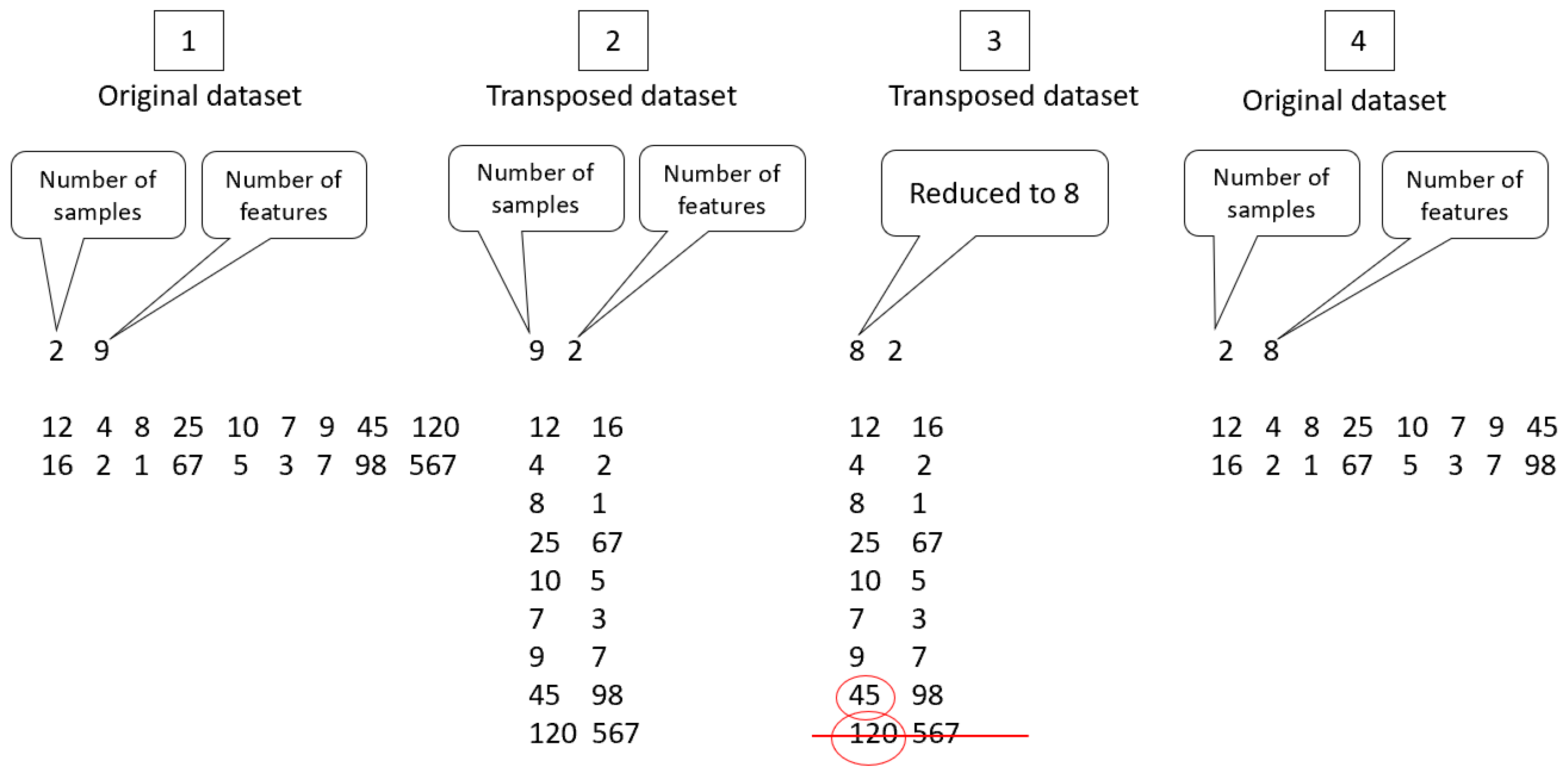
The detection of the outliers is univariate. First, let us represent the dataset as a matrix. The dataset matrix is transposed so that the rows represent the features (the attributes) and the columns are the samples. This is because the outliers can be found in the feature set of the original dataset (samples of the transposed dataset). Figure 2 shows an example of PPFS processing.
After transposing the dataset matrix, the PP index is chosen (either Friedman or Kurtosis) as well as the optimization method (either GA or Tribes). Then, the number of iterations and the number of runs are set (defined in the next section). Later, the optimization is applied to find the best projection a (see Section 4) associated with the best value of the PP index . The next step is to determine the outliers. For that, purpose the coordinate of the projected data are calculated according to Equation (1). In order to point out an observation (in the transposed dataset matrix) as an outlier, the rule based on k-sigma principle was applied. In fact, an observation is considered as an outlier when its distance to the mean is larger than 3 times the standard deviation of the projected data. Thus, the parameter k is set to 3 based on the recommendation of [37,38].
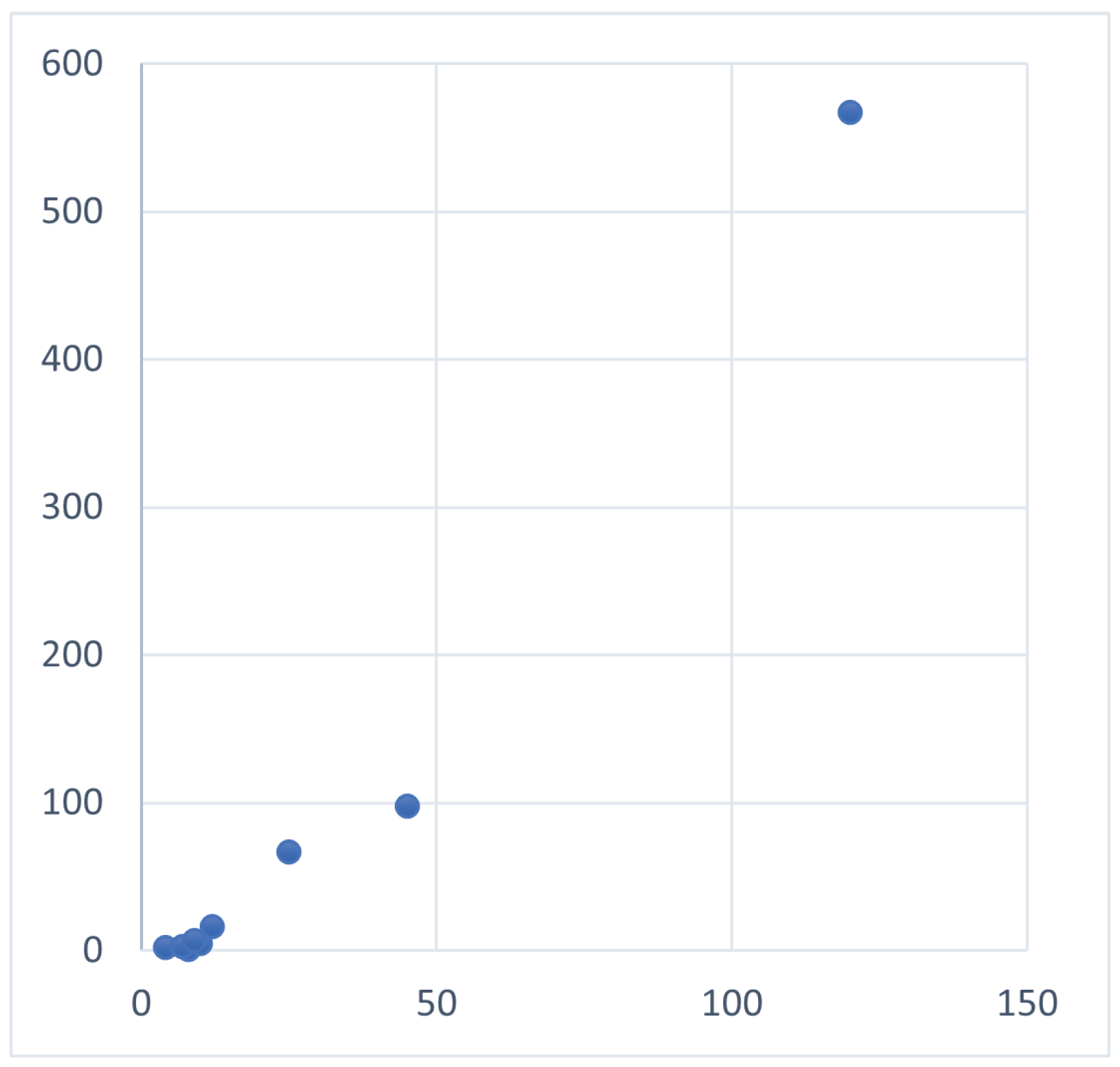
The optimization methods are performed several times (number of runs) to ensure that the obtained result is the best and cannot be changed. When selecting the best projection and determining the outliers, a threshold is set to confirm the outlying status of the recognized outliers. This threshold is set to half the number of runs. In fact, the proposed framework checks how many times these observations were detected as outliers throughout the runs. Thus, each outlier is associated with the frequency number showing how many times it was detected as outlier. In case of the previous example displayed in Figure 2, the last observation of the transposed matrix can be considered as an outlier because it is far from data points as displayed in Figure 3.
By applying PPFS, suppose that the number of runs is set to 100, and the two samples number 8 and 9, from the previous transposed dataset matrix example (see Figure 2) are detected as outliers. Therefore, the proposed technique will detect these two outliers with the number of times they were recognized as outliers after performing 100 runs. The sample number 8 will not be detected as an outlier, or it will be detected but with a frequency number less than the threshold (=50), while sample 9 will be detected with a frequency greater than 50 as it is considered as outlier. This frequency number ensures the status (outlier or not) of each observation. In this study, an outlier is confirmed if it is detected more than the fixed threshold (half the number of runs). The list of confirmed outliers corresponds to the non-relevant features in the original dataset.
Outlier Detection Using EPP-Lab
The extraction of the outliers is performed using EPP-Lab software available at https://www.researchgate.net/project/Projection-Pursuit (accessed on 22 July 2021) or https://github.com/fischuu/EPP-lab (accessed on 22 July 2021).
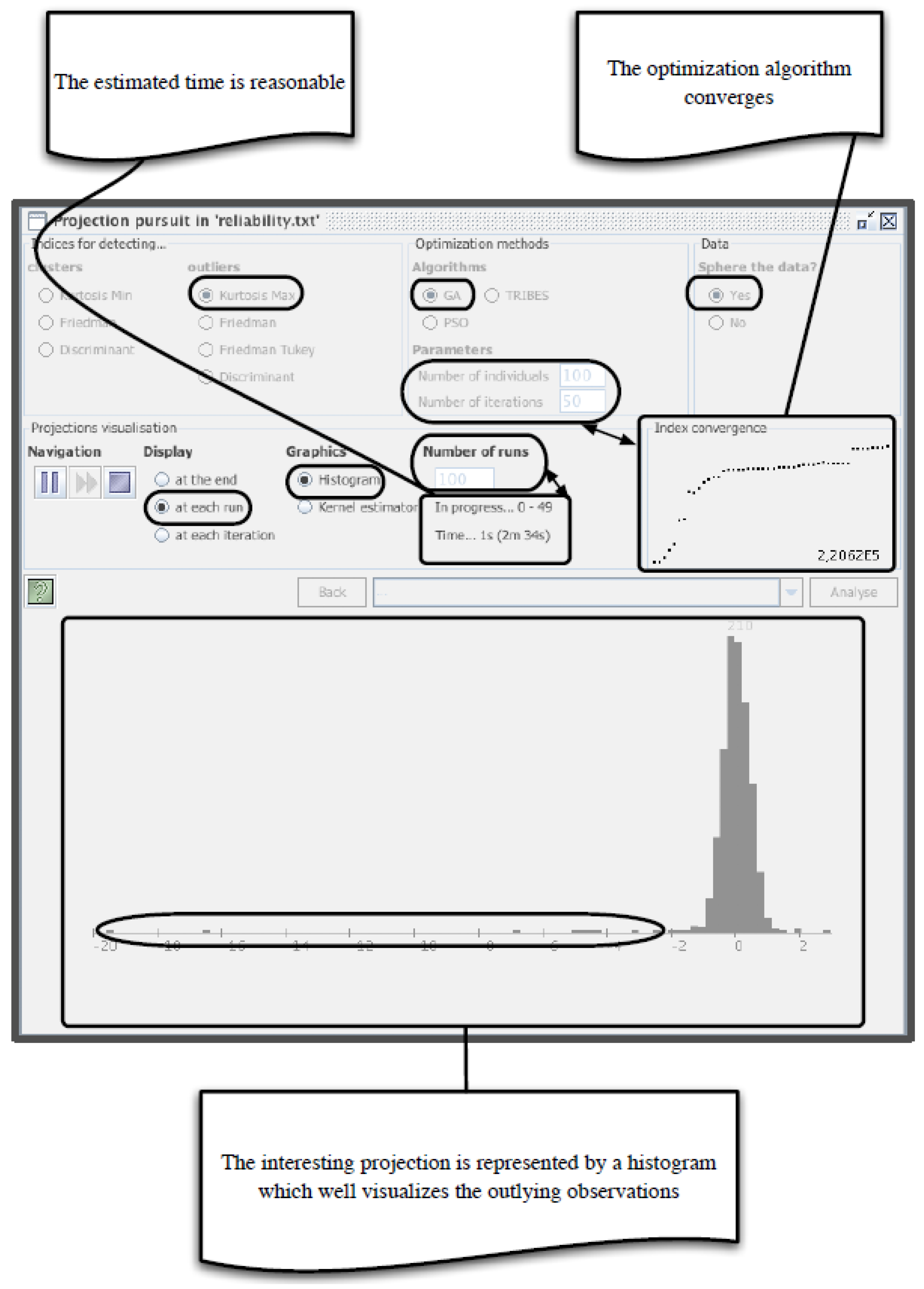
After the transposed dataset matrix is uploaded in EPP-Lab, the PP index is chosen (either Friedman or Kurtosis) as well as the optimization method (either GA or Tribes) from the EPP-Lab software. Then, the number of iterations and the number of runs are set (defined in the next section). Figure 4 shows the EPP-Lab interface used for this purpose.
After running, the best projection, the best values of the PP index obtained throughout the runs, and the projected data are provided. EPP-Lab allows the user to set the k parameter of the sigma rule. The software provides a list of detected outliers and the number of times (the frequency) they are detected as outliers. The functioning of EPP-Lab is described in [38].
6.2. Feature Selection
This stage involves removing the outliers obtained from the original dataset and keeping only the relevant features. Considering the previous example, feature 6 will be removed from the feature set of the original dataset, as shown in Figure 2. Therefore, the new dataset (after removing the irrelevant features) will be used in the classification phase.
6.3. Classification
This stage involves performing the classification of the dataset before and after removing the outliers (reducing the data dimentionality) using three classifiers, k-Nearest Neighbors (k-NN), Support Vector Machine (SVM), and Random Forest (RF) with ten-fold cross-validation. The reason behind the choice of these classifiers is that k-NN is the simplest classifier that is recommended for small datasets [46], while SVM and RN are well known for their efficiency in tackling large datasets [46,47].
6.4. Validation
The last step consists of validating the classification model using four classification measures including the accuracy, precision, recall, and F1 measure.
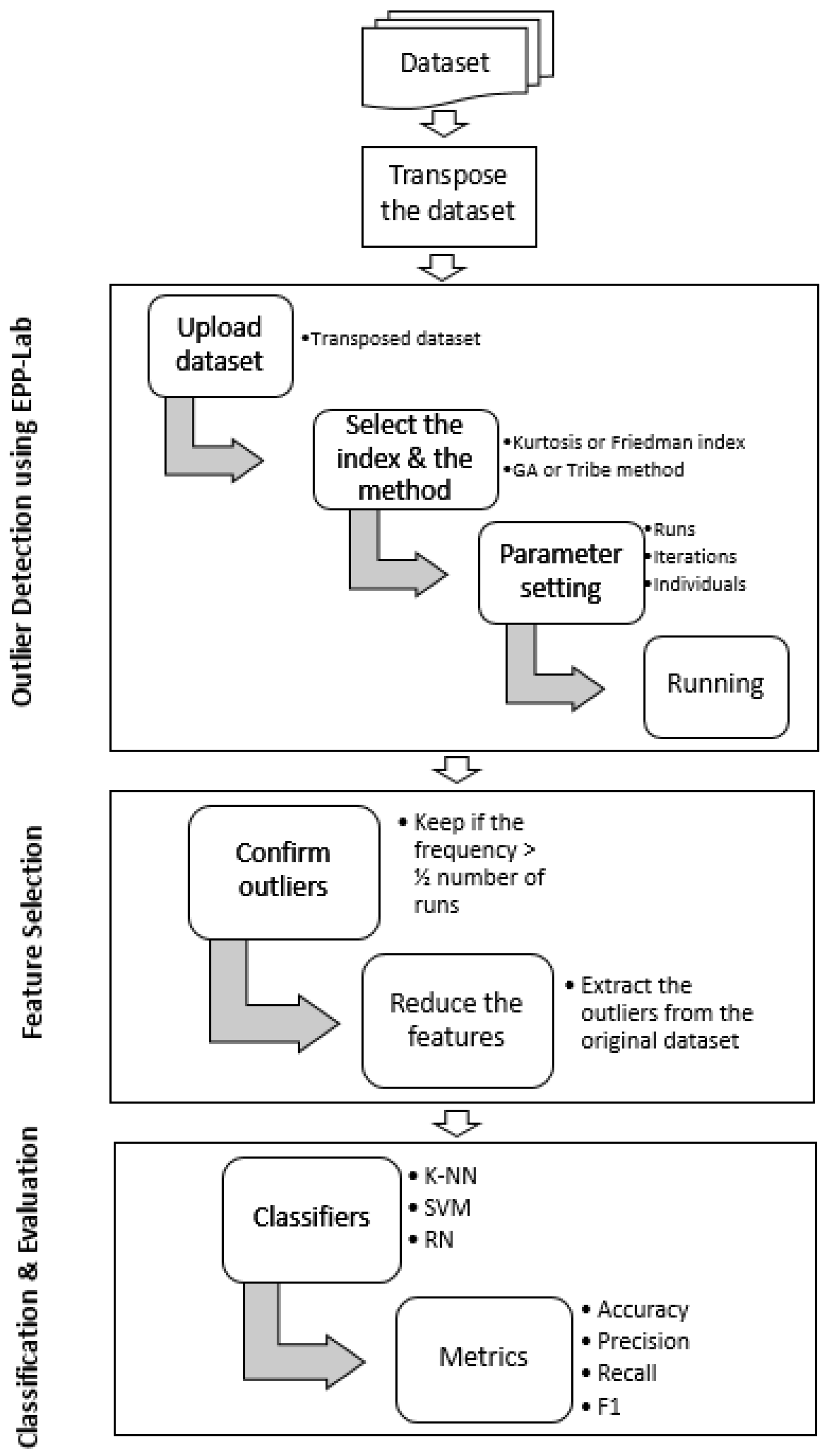
Figure 5 summarizes the four steps that define the proposed approach including transposing the dataset, detecting the outliers using EPP-Lab, FS, classification and evaluation.
7. Experimentation Results
The proposed outlier detection-based FS techniques (PPFS) were tested using a Dell XPS 9343 with an Intel core TM i7-5500U CPU 2.40 GHz and 8 GB RAM. In the following experimentation, 19 datasets (described in Table 2) were used to validate the effectiveness of this study. The first nine datasets are from the UCI repository (https://archive.ics.uci.edu/ml/datasets.php (accessed on 14 January 2021)). The next eight datasets are from (https://www.openml.org/search?q=australian&type=data (accessed on 14 January 2021)). Finally, August_senate_polls (August S.P) dataset is taken from https://data.world/fivethirtyeight/august-senate-polls (accessed on 14 January 2021), and Fifa2019 is from https://www.kaggle.com/karangadiya/fifa19 (accessed on 14 January 2021). August S.P contains polls from 1990 to 2016, the results of the election related to each poll, and the average error of each poll. This dataset is composed of three classes. The Fifa2019 dataset is composed of more than 13,000 instances and 80 attributes. An extensive preprocessing operation was applied to this dataset. Then, two classes were created in the body_type attribute, namely Lean and Normal, using R programming language.
As EPP-Lab software is used for outlier detection, only the number of iterations and the number of runs are set. All the parameters related to GA (set in EPP-Lab [38]) were not changed. This is why no validation phase for setting the parameters of GA is needed. In fact, for GA, the population is randomly generated with 50 individuals. The tournament selection was used with three individuals. The crossover was employed with two points, and the probability equals 0.65. The mutation is applied to all individuals with a probability 0.05. As stated before, the Tribes method does not require parameters. For the initialization phase, the EPP Lab randomly generates an initial solution (population) for each method. The numbers of iterations and runs are set to 100 according to the recommendations of [38]. The number of runs guarantees that the obtained results (the removed outliers) cannot be improved. It also allows determining the number of times a feature is detected as an outlier. The threshold that confirms the outlying status is then set to 50 (see Section 6.1). For more details, one can refer to [38,44].
Table 3 shows the parameters’ values.
In the classification stage, three classifiers are applied: Support Vector Machine (SVM) with a Linear kernel, the k Nearest Neighbors (k-NN), and the Random Forest (RF). R (version 3.5.1) is used for the classification step. The datasets are split into training (70%) and testing (30%). The split was done randomly by R using the “createDataPartition” function from the caret library. To validate the parameter setting of the classifiers, ten-fold Cross-Validation, repeated ten times, is applied to the training set. The accuracy with the largest value is used to select the optimal training model. The optimal model with its best parameters’ values is then used in the testing stage. The training and validation accuracy values are omitted to save space. The training set is centered and scaled.
For the k-NN classifier, several values of k were tested (between 5 and 200) for each dataset. For the RF classifier, the number of attributes used for splitting at each node in the tree was studied. The optimal training model was selected using the values (0.1, 0.8, 2, 6, 10). For the SVM classifier, the cost parameter was investigated, which is considered as the essential parameter for building the best useful model. After several experiments, the values (0.5, 1, 1.25, and 2) were used to select the optimal training model. Table 4 shows the obtained accuracy values for SVM using the four aforementioned values of the cost for the Breast Cancer dataset after applying PPFS-GAF. The final value used for the model was cost = 0.5. Note that this parameter setting approach was applied to the three classifiers before and after applying the four PPFS methods for all the datasets. Therefore, to save space, only Table 4 is shown.
7.1. Projection-Pursuit-Based Feature-Selection Techniques
The four PPFS methods include PP based on Friedman index and the GA optimization method (called GAF), PP based on Friedman index and the Tribes optimization method (called TF), PP based on Kurtosis index and the GA optimization method (GAK), and PP based on Kurtosis index and the Tribes optimization method (called TK). After detecting the outliers using each PPFS method, they were removed, and then the three classifiers were applied to determine the accuracy, precision, recall, and F1 measures for all the datasets, as explained in the Methodology section. Prior to starting the experiments, the features were numbered, starting from 1, according to their appearance in the dataset. For example, if a dataset had four features, then the features were numbered from 1 to 4 starting with the first feature in the dataset until the last one. Table 5 displays the number of outliers detected by each approach (column 4) for each dataset. In addition, the features detected as outliers and the number of times (over 100 runs) they were recognized as such (frequency) are shown in column 3. The last column yields the running time of PPFS to find out the outliers.
Most of the outliers are commonly revealed by the four approaches as shown in Column 3. Moreover, their frequency values are greater than the threshold (half of the number of runs = 50). For example, for the Diabetes dataset, the features 1, 2, 5, and 7 were detected as outliers by both PPFS-GAF and PPFS-TF. However, the features 2 and 7 were detected by the four PPFS methods. In addition, these features were recognized as outliers more than 68 times over 100 runs. Hence, the four features can be considered non-relevant and were removed from the dataset to perform the classification. The positive point in this result is that the four PPFS methods provide almost similar outputs. This fact confirms the consistency of the proposed study. The small difference can be explained by the behavior of the projection indices as well as the effect of the optimization methods. The Kurtosis index split the data into two unbalanced clusters, and the smallest one is considered to comprise outliers. The Friedman index detects the outliers by weighting distances in the center of the Normal distribution rather than in the tails [40]. For the optimization methods, GA is well-known in finding the best solution (the optimum or close to the optimum), whereas the Tribes is dedicated to finding local optima as well as the optimum. Therefore, combining these two optimization methods along with both PP indices does not yield exactly the same result; however, the accuracy and the different measures (precision, recall, and F1) provided by each classifier for the four approaches are slightly different for the used datasets. For the experiment time, EPP-Lab is fast when combining Tribes and the Kurtosis index [39]. The shortest average time noticed with the smallest dataset (Wine, 178 samples) was 79 ms using TK and 162 ms using TF. With the largest dataset, Fifa2019, there were 13,000 samples and 80 features, while Colon had 62 samples and 2000 features. TK for Fifa2019 spent an average of 12 s 580 ms, whereas TF took an average of 44 s 143 ms. TK for Colon was 1 s 654 ms, and TF was 6 s 443 ms. Again, the running time does not show a major difference (see Table 5).
Table 6 presents the accuracy, precision, recall, and the F1 values of each classifier before and after applying PPFS methods (columns 3–6 for k-NN, columns 7–10 for SVM, and columns 11–14 for RF). The PPFS methods have globally improved the classification accuracy compared to the accuracy obtained without applying FS. The accuracy obtained using k-NN (resp. SVM and RF) indicates an improvement rate ranging between 0.08 and 6.79 for 9 datasets, while the accuracy for SVM and RF were 0.36–12.9 and 0.01–12.7, respectively, for 16 datasets each. This result is explained by the fact that k-NN is not always efficient with large and noisy datasets. The classification accuracy of the datasets that is not enhanced with k-NN achieved a significant improvement rate with the other classifiers. This is the case for Wine, Spam, August S.P, Diabetes, Australian, Glass, and Ionosphere datasets.
The PPFS methods also managed well for the Fifa2019 dataset even though the accuracy remains below 70%. This dataset is large and required massive preprocessing efforts. However, PPFS methods did not enhance the accuracy of the Waveform and Segment datasets using the three classifiers because Waveform contains 40 features, all of which include noise, especially the last 19, which are all noise, and Segment contains many instances of noise. PPFS did not remove all these noise features.
Moreover, considering the results of the three classifiers, the classification accuracy of some datasets was enhanced, but they remained below or around 70%. This is the case of Liver D., Vehicle (enhanced only once reaching 83.33%), Diabetes (enhanced only once reaching 81.30%), Glass, and Fifa2019. To improve the results, it recommended to preprocess the datasets and/or apply centering and sphering procedure [37] before peforming PPFS.
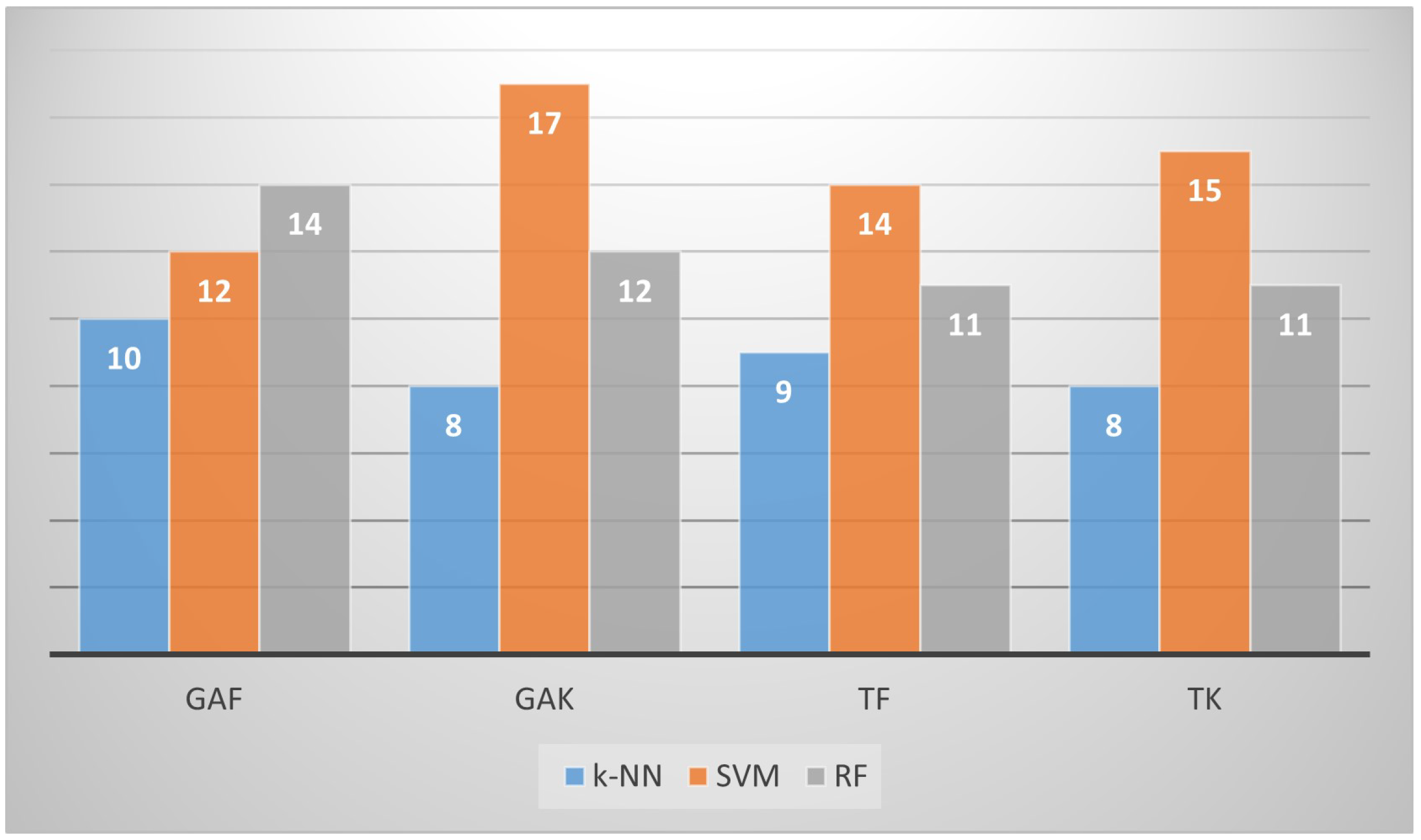
The four proposed PPFS methods provided approaching accuracy, precision, recall, and F1 values for each dataset. This confirms the consistency of PPFS again. Figure 6 shows the number of times each PPFS method enhances the classification accuracy (compared to that obtained without applying any FS method) using the three classifiers for all datasets. As displayed in this figure, GAF and GAK performed well at 36 and 37 times, respectively, using the three classifiers. In fact, GAF enhanced the accuracy 10 times with k-NN, 12 times with SVM, and 14 times with RF. TF and TK yielded similar results (34 times). On the other hand, the SVM classifier performed well with all the PPFS methods for all the datasets. It enhanced the results 58 times. The RF is a comparative classifier as it enhanced the accuracy results 48 times using the PPFS for all the datasets. The k-NN does not perform well with large datasets. It improved the accuracy 35 times using all the PPFS methods for all the datasets. Consequently, SVM can be considered as the classifier providing the best results.
7.2. What Is the Best PPFS Technique?
It is necessary to show that the results of the PPFS approaches are equivalent. To do this, the non-parametric statistical test “Friedman” was employed with a significance level of . This test is conducted with the best classification accuracy obtained by SVM for all the datasets after performing PPFS. The test does not adopt a normal distribution assumption [48].
It is worth knowing that the Friedman test [48] is different from the Friedman index used in PP [40]. The Friedman index is defined in Section 4, and Friedman test shows the existence of a significant statistical difference between the methods.
The Friedman test provides two main results, the p-value and the effect size. If the obtained p-value is less than the significance level (), then the statistical hypothesis (that the PPFS methods are equivalent) is rejected. The effect size has a value ranging between 0 (corresponding to no relationship) and 1 (stating an ideal relationship). The Friedman test resulted in and , with an effect size . According to the , the hypothesis is not rejected. Moreover, the effect size is small. Consequently, there is no statistical difference between the PPFS methods. The obtained PPFS results are equivalent.
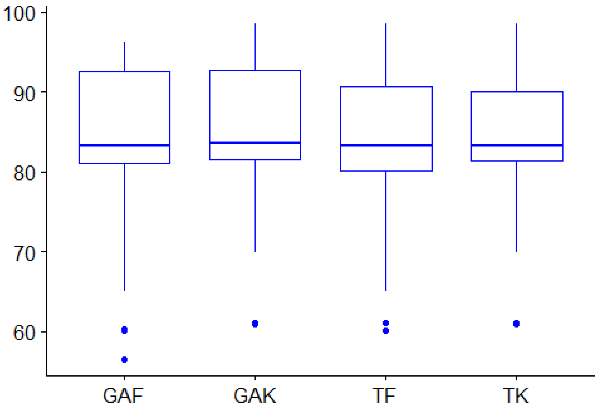
Figure 7 displays the boxplot of the accuracy obtained by SVM after using the PPFS methods for all the datasets. The y-axis represents the minimum, first quartile, median, third quartile, and maximum value of the accuracy values. As indicated, the four PPFS have a similar median (the line inside the box) equal to for GAF, TF, and TK, for GAK. As the , the dissimilarity between the median values are not statistically significant. This confirms that the PPFS techniques are equivalent and that their results are statistically significant. Furthermore, the mean values of the four PPFS do not show a significant difference. The lowest value was provided by GAF (82.0), whereas the highest mean was obtained by GAK (84.2). TF yielded 82.6 and TK 83.3.
7.3. Comparison Study
The comparison study was performed based on three wrapper and five filter-based FS methods. Unfortunately, the existing embedded FS methods did not use the available datasets or apply clustering techniques (instead of classification techniques). Furthermore, the related work applying outlier detection to select the relevant features did not use the available data, and their evaluation measures are different from those used in this article.
The first comparison study consisted of applying the Correlation (CFS), Principal Component Analysis (PCA), Gain ratio, the Mutual Information, and Gini index FS techniques. The reason behind this choice is that PCA belongs to the same family of the PP and the other FS are well-known filter FS methods. The implementation of the filter FS techniques was performed using both FSelector and FSinR R packages [11]. The Gain ratio, Mutual Information, and Gini index were applied using the Sequential Forward Selection (FSF) search method as it provided better results than Sequential Backward Selection (SBS) and Breadth First Search (BFS). In addition, the FSF search method was the fastest.
Table 7 displays the classification accuracy obtained by SVM (as it is the best classifier in this study) after applying the four PPFS methods along with the five filter FS for all the datasets. As shown in this table, the four PPFS outperformed all the Filter FS for 15 datasets (over 19 datasets). The accuracy improvement rate ranges between 0.76% and 30.64%. However, PCA managed well in eliminating the noisy features of Waveform dataset. In addition, it enhanced the accuracy of Sonar dataset despite its correlated features. This is due to its process in projecting the feature space into a new low-dimensional feature space without being affected by the noise or high correlation. Furthermore, CFS also improved the accuracy of Sonar dataset. This is done thanks to the concept of removing the correlated features. Besides, Mutual Information and Gini Index outperformed the PPFS methods when tackling the Spam dataset. Moreover, CFS, Gain ratio, Mutual Information, and Gini index (resp. CFS) yielded similar results to the four PPFS methods when handling the Climate (resp. Heart) dataset. For the Colon dataset, the last three FS methods did not manage to find the relevant features. For the running time, the five filter FS are similar to PPFS in terms of speed, except when handling Spam, Colon, and Fifa2019. For these datasets, the filter FS took an average of 12 min and 10 s compared to PPFS, which took an average of 7 s.
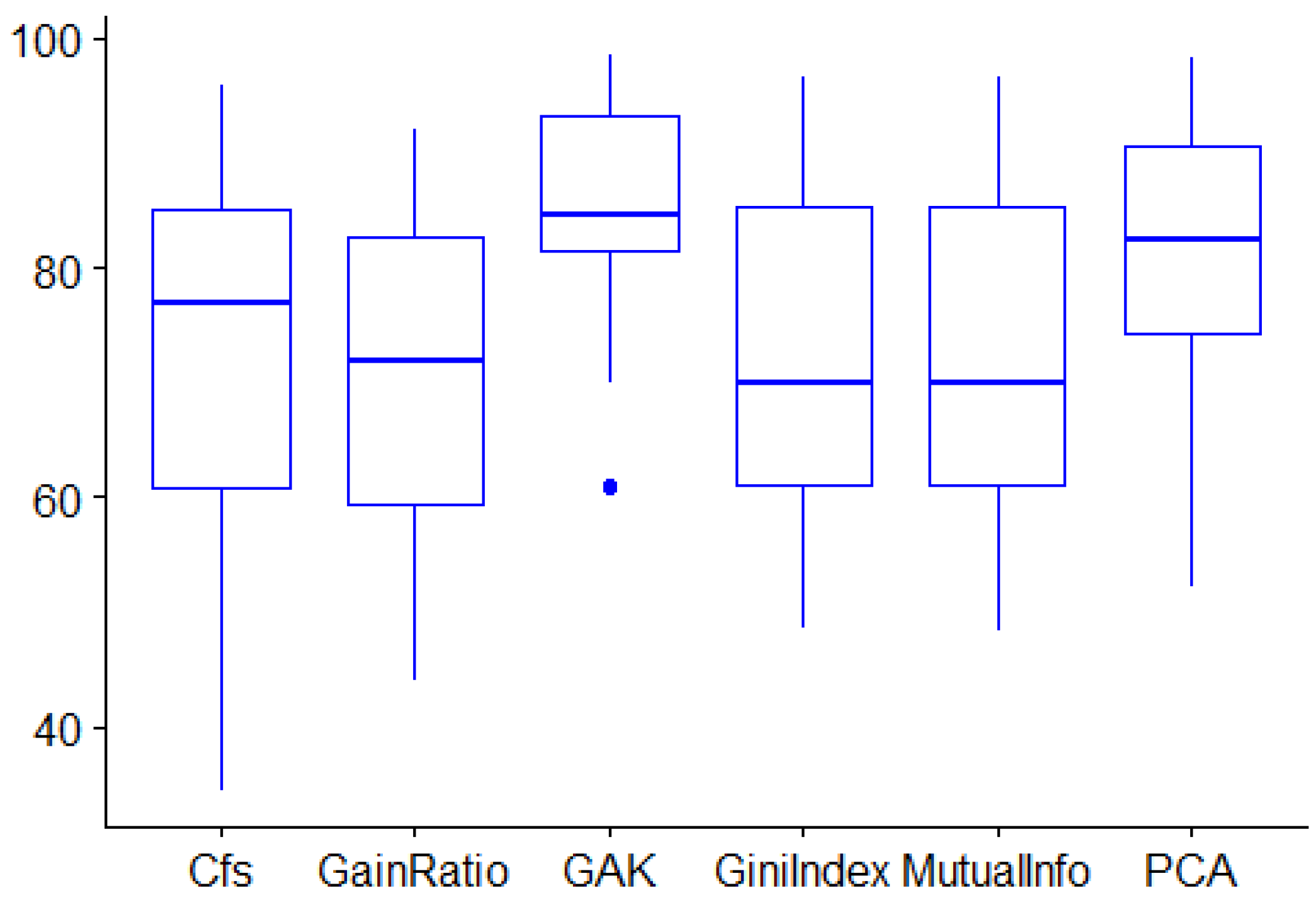
To show the statistical significance of the obtained results, the same experiment discussed in Section 7.2 was performed. It aimed to show the existence of a significant statistical difference between the methods. As the PPFS methods are equivalent, only GAK was used. Table 8 displays the mean and median of the accuracy values obtained by SVM classifier after applying GAK and the five filter FS methods. These results are visually shown in Figure 8. As indicated, the median and the mean of GAK are greater than those of the four filter methods, but slightly different from those of PCA. Moreover, the Friedman test was applied with a confidence level of 0.01. The achieved , , with an effect size (small effect), which means that there is no relationship. Thus, the statistical hypothesis (the methods are not statistically different) is rejected since the is less than the significant level and the effect size is small.
This result indicates that the methods are statistically different.
Now, to demonstrate the differences between each pair of methods, the Friedman test was followed by the pairwise Wilcoxon signed-rank test. Table 8 (see the first line) pointed out the calculated between GAK and the filter methods. As displayed, GAK, CFS, and PCA are competitive methods. This is because the hypothesis is not rejected (GAK is statistically different from CFS and PCA) due to the not being less than the significance level . However, GAK is better than Gain Ratio, Mutual Information, and Gini index FS methods, since their p-value is less than . Consequently, GAK outperforms Gain Ratio, Mutual Information, and Gini index, but it is competitive with PCA and CFS. This result is again confirmed with the medians and the means computed in Table 8.
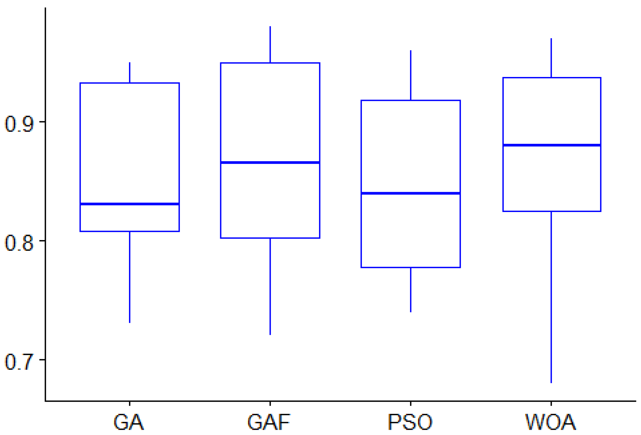
The second comparison study involved comparing PPFS approaches with three wrapper-based FS methods published in [14], named Enhanced Whale Optimization Algorithm (WOA-CM), GA, and PSO using k-NN. Note that GA is also employed in GAF and GAK, and Tribes is one variant of PSO used in TF and TK. Table 9 and Figure 9 show the classification accuracy obtained by k-NN after applying PPFS techniques along with the three wrapper methods using eight UCI datasets. The PPFS approaches outperformed the wrapper FS methods on five datasets. However, only WOA outperformed the four PPFS methods with an improvement of 5.06% for Ionosphere, 13.12% for Colon, and 16.09% for the Sonar datasets. In addition, the three wrapper FS outperformed the four PPFS methods when handling the Colon dataset. The reason behind this success is that WOA is mainly based on the exploration and exploitation concepts leading to the global search. This aspect allowed WOA to find out the optimal solutions for the Waveform, Colon, and Sonar datasets in revealing the important features despite the noise and high correlation containing in these datasets.
Since the number of datasets used in this comparison study is small (eight datasets), the result of the statistical tests (Friedman or Wilcoxon) might be inaccurate [48]. Therefore, their results were omitted. However, the median and the mean of the accuracy values obtained by k-NN after applying GAF, WOA, PSO, and GA were calculated and displayed in Table 10. In addition, the Boxplot of these four methods was presented in Figure 10. As displayed, the mean and the median of the accuracy values obtained by GAF are higher than those obtained by PSO and GA, but somewhat similar to WOA. Therefore, it is worth mentioning that GAF yielded results better than or comparable to the aforementioned FS. Therefore, PPFS methods are competitive methods.
7.4. Discussion
Many experiments were performed in this paper to fulfill the four reseach objectives. Firstly, the related works were deeply investigated to bring out their limitations. Consequently, the first objective was achieved.
To prove the efficacy of these four PPFS, nineteen datasets and three classifiers were utilized. The first experiment consists of showing the detected outliers for the nineteen datasets using the four FS methods. It was shown that the PPFS methods provide equivalent results in terms of the detecting outliers. In addition, the detection frequency of most of the outliers reached 80% using the four PPFS methods. This confirms that they are outliers. To show that the detected outliers correspond to non-relevant features, classification was performed on the datasets before and after applying the four PPFS methods. The results showed that the classification performance along with the precision, the recall, and the F1 measure were superior when applying PPFS. The k-NN achieved an improvement, reaching 6.79 for 11 datasets. The SVM and RN enhanced the results of 16 datasets, with an improvement reaching 12.91 and 12.4, respectively. Hence, SVM was selected as the best classifier for this study. Although the proposed PPFS did not improve the accuracy of the Waveform and Segment datasets, they enhanced the classification accuracy for most of the datasets. This allowed the second and third objectives to be realized.
On the other hand, the success of this study could not be realized without the utilization of EPP-Lab software. Therefore, EPP-Lab is efficient in detecting the non-important features. This software is open-source and can be used as a desktop application in any environment. This is the fourth objective of the present study.
One of the main experiments performed in this article was to show that the four presented PPFS methods provide equivalent results. This was carried out through the Friedman test. The test’s result indicated that the p-value is greater than the significace level and that the effect size is small. Consequently, the hypothesis is not rejected, and hence the difference between the PPFS results is not statistically significant. This experiment realized the fifth objective.
To demonstrate that the four PPFS are competitive FS methods, two comparison studies were performed. The first comparison included applying five filter FS methods (CFS, PCA, Gain Ratio, Mutual Information, Gini Index) using all the datasets. The results showed that CFS was superior to the four PPFS methods when testing only the Sonar dataset. PCA was also superior to the four PPFS methods when testing both the Waveform and Sonar datasets. Again, Mutual Information and Gini Index outperformed the PPFS for the Spam dataset. As stated previously, these three datasets have noise and high correlation, which negatively affect PPFS in enhancing the classification accuracy. These limitations deserve further investigation. The classification accuracy results of PPFS-GAK and the five Filter FS methods were used to compute the Friedman and pairwise Wilcoxon tests. The statistical results show that GAK is superior to Mutual Information, Gain Ratio, and Gini Index but equivalent to PCA and CFS.
The second comparison involved comparing PPFS with three wrapper FS methods, called WOA, PSO, and GA, using eight datasets. The four PPFS methods performed better than the three wrapper FS using five datasets. However, WOA surpassed all the FS methods using Sonar, Waveform, and Colon datasets. Again, the PPFS methods failed in enhancing the accuracy of these three datasets. Like the first comparison study, the statistical analysis validated the significant results of the PPFS methods. Finally, the last objective was achieved by demonstrating the efficiency of the PPFS methods. To sum up, the aforementioned experiments successfully carried out the research objectives of this study.
In the following, the research impacts, the advantages, and the limitations of PPFS methods are discussed.
7.4.1. Research Impacts
The research impacts of PPFS methods are important and deserve to be addressed:
- They contribute to the scientific society by providing a new PPFS model that overcomes the limitations of the existing FS methods.
- They provide four FS techniques that enhance the classification accuracy by an average of 6.64%.
- They contribute to technological development by providing EPP-Lab software handling FS.
- They contribute to decision making by providing four PPFS methods yielding different but equivalent results.
7.4.2. Advantages and Liminations of PPFS
The present research has six main advantages.
- PPFS methods are competitive and efficient FS methods.
- The four PPFS methods are different but provide similar results. The user can either apply all of them and choose the suitable result or use only one of them.
- PPFS methods can be used directly through EPP-Lab software.
- The EPP-Lab can be used to avoid the parameter setting of the optimization methods.
- PPFS methods provide a list of outliers, and their frequency allows validating the non-relevant features.
- EPP-Lab is an open-source desktop application, downloadable in any environment.
In spite of the previous advantages, PPFS have two limitations.
- PPFS failed to find the non-significant features when most of the features are highly correlated or include noise.
- PPFS methods do not work well when the dataset is binary (the values of features’ vectors are either 0 or 1).
8. Conclusions
The present study proposed four FS methods based on outliers detection using the Project Pursuit. Two PP indices along with two AI optimization methods were used to find the optimal projections that reveal the outliers. The proposed PPFS methods were validated using three classifiers and 19 datasets. They yielded promising results.Moreover, these methods were successfully compared with three Wrapper FS methods on eight datasets. They also yielded the best or equivalent accuracy against five Filter FS techniques on 15 datasets (among 19 datasets). Statistical analysis was performed and showed that PPFS are equivalent, and their results are statistically significant. It is also demonstrated that PPFS are comparative with PCA, CFS, and WOA. Therefore, our assumption to consider the outlier detection methods for revealing the irrelevant features from a dataset to increase the classification accuracy was validated. For the computation time, PPFS was faster than the five Filter FS methods when handling large datasets (Colon, Spam, and Fifa2019).
However, no computation time was reported for the three wrapper FS methods. Furthermore, PPFS yielded promising results in handling a large dataset reaching 13,000 instances (Fifa2019 dataset) and 2000 features (Colon dataset). The only limitation of this study is not getting the best result when dealing with the Waveform and Segment dataset. Hence, some future research directions are suggested:
- Make the dataset spherical before seeking the outliers [27] to reduce the noise.
- Use another optimization method such as PSO, which is already available in EPP-Lab.
- Use large datasets reaching 30,000 features to test the extent of PPFS in enhancing accuracy.
- Explore other PP indices such as Friedman Turkey and Discriminant indices.
- Investigate other Machine Learning classifiers.
Funding
The authors would like to acknowledge the support of Prince Sultan University for paying the Article Processing Charges (APC) of this publication.
Institutional Review Board Statement
Not applicable.
Informed Consent Statement
Not applicable.
Data Availability Statement
The links to datasets used in this study are provided in Section 7.
Acknowledgments
The author would like to acknowledge the support of Prince Sultan University for paying the Article Processing Charges (APC) of this publication. This work was also supported by Artificial Intelligence and Data Analytics Lab (AIDA), Prince Sultan University, Riyadh, Saudi Arabia.
Conflicts of Interest
The authors declare no conflict of interest.
Abbreviations
All the abbreviations used in this paper are defined below.
| FS | Feature Selection |
| PP | Projection Pursuit |
| PPFS | Project Pursuit based Feature Selection |
| AI | Artificial Intelligence |
| GA | Genetic Algorithms |
| PSO | Particle Swarm Optimization |
| EPP-Lab | Exploratory Projection Pursuit Laboratory |
| PPFS-GAF | Projection-Pursuit-based Feature Selection |
| using Genetic Algorithm and Friedman index | |
| PPFS-GAK | Projection-Pursuit-based Feature Selection |
| using Genetic Algorithm and Kurtosis index | |
| PPFS-TF | Projection-Pursuit-based Feature Selection |
| using Tribes and Friedman index | |
| PPFS-TK | Projection-Pursuit-based Feature Selection |
| using Tribes and Kurtosis index | |
| LASSO | Least Absolute Shrinkage and Selection Operator |
| LR | Linear Regression |
| CV | Cross Validation |
| k-NN | K-Nearest Neighbor |
| SVM | Support Vector Machine |
| RF | Random Forest |
| PCA | Principal Component Analysis |
| CFS | Correlation Feature Selection |
| WOA | Whale Optimization Algorithm |
| Accu | Accuracy |
| Prec | Precision |
| Rec | Recall |
| mutualInfo | Mutual Information |
References
- Fukumizu, K.; Bach, F.R.; Jordan, M.I. Dimensionality reduction for supervised learning with reproducing kernel hilbert spaces. J. Mach. Learn. Res. 2004, 5, 73–99. [Google Scholar]
- Sophian, A.; Tian, G.Y.; Taylor, D.; Rudlin, J. A feature extraction technique based on principal component analysis for pulsed Eddy current NDT. NDT E Int. J. 2003, 36, 37–41. [Google Scholar] [CrossRef]
- Scholkopf, B.; Smola, A.; Muller, K.-R. Nonlinear component analysis as a kernel eigenvalue problem. Neural Comput. J. 1998, 10, 1299–1319. [Google Scholar] [CrossRef] [Green Version]
- Chandrashekar, G.; Sahin, F. Survey on feature selection methods. J. Comput. Electr. Eng. 2014, 40, 16–28. [Google Scholar] [CrossRef]
- Guyon, I.; Elisseeff, A. An introduction to variable and feature selection. J. Mach. Learn. Res. 2003, 3, 57–82. [Google Scholar]
- Taminau, J.L.; Meganck, S.; Steenhoff, D.; Coletta, A.; Molter, C. A survey on filter techniques for feature selection in gene expression microarray analysis. IEEE/ACM Trans. Comput. Biol. Bioinform. 2012, 9, 6–19. [Google Scholar]
- Eom, J.; Zhang, B. PubMiner: Machine learning-based text mining for biomedical information analysis. Lect. Notes Artif. Intell. 2000, 3192, 216–225. [Google Scholar]
- Larabi-Marie-Sainte, S.; Ghouzali, S. Multi-Objective Particle Swarm Optimization-based Feature Selection for Face Recognition. Stud. Inform. Control. J. 2020, 29, 99–109. [Google Scholar] [CrossRef]
- Larabi-Marie-Sainte, S.; Alayani, N. Firefly Algorithm based Feature Selection for Arabic Text Classification. J. King Saud Univ. Comput. Inf. Sci. (JKSUCIS) 2020, 32, 320–328. [Google Scholar] [CrossRef]
- Wen, J.; Canbing, L.; Rui, L. A Heuristic Feature Selection Approach for Text Categorization by Using Chaos Optimization and Genetic Algorithm. Math. Probl. Eng. 2013, 2013. [Google Scholar] [CrossRef] [Green Version]
- Aragon-Royon, F.; Jimenez-Vilchez, A.; Arauzo-Azofra, A.; Benitez, J.M. FSINR: An exhaustive package for feature selection. arXiv 2020, arXiv:2002.10330v1. [Google Scholar]
- Rattanawadee, P.; Anongnart, S. Wrapper Feature Subset Selection for Dimension Reduction Based on Ensemble Learning Algorithm. Procedia Comput. Sci. 2015, 72, 162–169. [Google Scholar]
- Agrawala, R.K.; Kaur, B.; Sharma, S. Quantum based Whale Optimization Algorithm for wrapper feature selection. Appl. Soft Comput. J. 2020, 89, 106092. [Google Scholar] [CrossRef]
- Mafarja, M.; Mirjalili, S. Whale optimization approaches for wrapper feature selection. Appl. Soft Comput. J. 2018, 62, 441–453. [Google Scholar] [CrossRef]
- Gokalp, O.; Tasci, E.; Ugur, A. A novel wrapper feature selection algorithm based on iterated greedy metaheuristic for sentiment classification. Expert Syst. Appl. 2020, 146, 113–176. [Google Scholar] [CrossRef]
- Xu, T.; Feng, Z.H.; Wu, X.J.; Kittler, J. Learning Adaptive Discriminative Correlation Filters via Temporal Consistency Preserving Spatial Feature Selection for Robust Visual Object Tracking. IEEE Trans. Image Process. J. 2019, 28, 5596–5609. [Google Scholar] [CrossRef] [PubMed] [Green Version]
- Bommerta, A.; Sun, X.; Bischl, B.; Rahnenführer, J.; Lang, M. Benchmark for filter methods for feature selection in high-dimensional classification data. Comput. Stat. Data Anal. J. 2020, 143. [Google Scholar] [CrossRef]
- Wang, Y.; Tao, L. Local feature selection based on artificial immune system for classification. Appl. Soft Comput. J. 2020, 87, 105989. [Google Scholar] [CrossRef]
- Cai, J.; Hu, L.; Liu, Z.; Zhou, K.; Zhang, H. An Embedded Feature Selection and Multi-Class Classification Method for Detection of the Progression from Mild Cognitive Impairment to Alzheimer’s Disease. J. Med. Imaging Health Inform. 2020, 10, 370–379. [Google Scholar] [CrossRef]
- Guo, Y.; Chung, F.-L.; Li, G.; Zhang, L. Multi-Label Bioinformatics Data Classification With Ensemble Embedded Feature Selection. IEEE Access J. 2019, 7, 103863–103875. [Google Scholar] [CrossRef]
- Azmandian, F.; Dy, J.G.; Aslam, J.A.; Kaeli, D.R. Local Kernel Density Ratio-Based Feature Selection for Outlier Detection. In Proceedings of the Asian Conference on Machine Learning, Singapore, 4–6 November 2012; Volume 25, pp. 49–64. [Google Scholar]
- Suresh, M.S.S.; Narayanan, A. Improving Classification Accuracy Using Combined Filter+Wrapper Feature Selection Technique. In Proceedings of the 2019 IEEE International Conference on Electrical, Computer and Communication Technologies (ICECCT), Coimbatore, India, 20–22 February 2019; pp. 1–6. [Google Scholar]
- Hallac, D.; Leskovec, J.; Boyd, S. Network lasso: Clustering and optimization in large graphs. In Proceedings of the KDD, Sydney, Australia, 10–13 August 2015. [Google Scholar]
- Osanaiy, O.; Cai, H.; Raymond-Choo, K.K.; Dehghantanha, A.; Xu, Z.; Dlodlo, M. Ensemble-based multi-filter feature selection method for DDoS detection in cloud computing. EURASIP J. Wirel. Commun. Netw. 2016, 130, 1–10. [Google Scholar] [CrossRef] [Green Version]
- Hadi, S.; Imon, A.H.M.R.; Werner, M. Detection of outliers. Wiley Interdiscip. Rev. Comput. Stat. 2009, 1, 57–70. [Google Scholar] [CrossRef]
- Ruiz-Gazen, A.; Larabi-Marie-Sainte, S.; Berro, A. Detecting Multivariate Outliers Using Projection Pursuit with Particle Swarm Optimization. In Proceedings of the 19th International Conference on Computational Statistics (Book Chapter), Paris, France, 22–27 August 2010; pp. 89–98. [Google Scholar]
- Berro, A.; Larabi-Marie-Sainte, S.; Ruiz-Gazen, A. Genetic Algorithms and Particle rm Optimization for Exploratory Projection Pursuit. Ann. Math. Artiffitial Intell. J. 2010, 60, 153–178. [Google Scholar] [CrossRef]
- Yang, Q.; Singh, J.; Lee, J. Isolation-based feature Selection for Unsupervised Outlier Detection. In Proceedings of the Annual Conference of the PHM Society, Scottsdale, AZ, USA, 21–22 September 2019; Volume 11. [Google Scholar]
- Kovarasan, R.K.; Rajkumar, M. An Effective Intrusion Detection System Using Flawless Feature Selection, Outlier Detection and Classification. In Progress in Advanced Computing and Intelligent Engineering. Advances in Intelligent Systems and Computing; Pati, B., Panigrahi, C., Misra, S., Pujari, A., Bakshi, S., Eds.; Springer: Berlin/Heidelberg, Germany, 2019; p. 713. [Google Scholar]
- Karthikeyan, G.; Balasubramanie, P. Robust Feature Selection Model for Outlier Detection Using Fuzzy Clustering and Rule Mining. Int. J. Appl. Eng. Res. 2017, 12, 7019–7028. [Google Scholar]
- Pang, G.; Cao, L.; Chen, L. Learning Homophily Couplings from Non-IID Data for Joint Feature Selection and Noise-Resilient Outlier Detection. In Proceedings of the Twenty-Sixth International Joint Conference on Artificial Intelligence (IJCAI-17), New York, NY, USA, 9–15 July 2016. [Google Scholar]
- Solorio-Fernández, S.; Carrasco-Ochoa, J.A.; Martínez-Trinidad, J.F. A new hybrid filter–wrapper feature selection method for clustering based on ranking. Neurocomput. J. 2016, 214, 866–880. [Google Scholar] [CrossRef]
- Zhen, L.; Xin, L.; Jin, M.; Hui, G. An Optimized Computational Framework for Isolation Forest. Math. Probl. Eng. 2018, 2018. [Google Scholar] [CrossRef] [Green Version]
- Koupaie, H.M.; Suhaimi, I.; Hosseinkhani, J. Outlier Detection in Stream Data by Machine Learning and Feature Selection Methods. Int. J. Adv. Comput. Sci. Inf. Technol. (IJACSIT) 2013, 2, 17–24. [Google Scholar]
- Huber, P. Projection pursuit. Ann. Stat. 1985, 13, 435–475. [Google Scholar] [CrossRef]
- Jones, M.; Sibson, R. What is projection pursuit? (With discussion). J. R. Stat. Soc. A 1987, 150, 1–36. [Google Scholar] [CrossRef]
- Larabi-Marie-Sainte, S. Biologically Inspired Algorithms for Exploratory Projection Pursuit. Ph.D. Thesis, Toulouse 1 University (Tolbiac), Toulouse, France, 2011. Available online: https://scanr.enseignementsup-recherche.gouv.fr/publication/these2011TOU10021 (accessed on 20 July 2021).
- Larabi-Marie-Sainte, S. Detection and visualization of non-linear structures in large datasets using Exploratory Projection Pursuit Laboratory (EPP-Lab) software. J. King Saud Univ. Comput. Inf. Sci. 2017, 29, 2–18. [Google Scholar]
- Penã, P.; Prieto, F. Cluster Identification using projections. J. Am. Stat. Assoc. 2001, 456, 1433–1445. [Google Scholar] [CrossRef] [Green Version]
- Friedman, J. Exploratory Projection Pursuit. Am. Stat. Assoc. 1987, 82, 249–266. [Google Scholar] [CrossRef]
- Sun, J. Some practical aspects of exploratory projection pursuit. SIAM J. Sci. Comput. 1993, 14, 68–80. [Google Scholar] [CrossRef]
- Holland, J.H. Adaptation in Natural and Artificial Systems; University of Michigan Press: Ann Harbor, MI, USA, 1975. [Google Scholar]
- Kennedy, J.; Eberhart, R. Swarm Intelligence; Shi, Y., Ed.; Springer: Boston, MA, USA, 1995. [Google Scholar]
- Larabi-Marie-Sainte, S.; Berro, A.; Ruiz-Gazen, A. An efficient Optimization Method for Revealing Local optima of Projection Pursuit Indices. In Proceedings of the Swarm Intelligent, ANTS2010, Brussels, Belgium, 8–10 September 2010; pp. 60–71. [Google Scholar]
- Clerc, M. Particle swarm optimization. In International Scientific and Technical Encyclopaedia; Wiley: Hoboken, NJ, USA, 2006. [Google Scholar]
- Tomar, A.; Nagpal, A. Comparing Accuracy of K-Nearest-Neighbor and Support-Vector-Machines for Age Estimation. Int. J. Eng. Trends Technol. (IJETT) 2016, 38, 326–329. [Google Scholar] [CrossRef]
- Huang, M.W.; Chen, C.W.; Lin, W.C.; Ke, S.W.; Tsai, C.F. SVM and SVM Ensembles in Breast Cancer Prediction. PLoS ONE 2017, 12. [Google Scholar] [CrossRef]
- Derrac, J.; Garcia, S.; Molina, D.; Herrera, F. A practical tutorial on the use of nonparametric statistical tests as a methodology for comparing evolutionary and swarm intelligence algorithms. J. Swarm Evol. Comput. 2011, 1, 3–18. [Google Scholar] [CrossRef]
Figure 1.
Feature selection categories.

Figure 2.
An example of PPFS Processing.

Figure 3.
Representation of the transposed matrix of the above example.

Figure 4.
Outlier detection interface using EPP-Lab [37].
Figure 4.
Outlier detection interface using EPP-Lab [37].

Figure 5.
Projection Pursuit-based feature-selection approach.

Figure 6.
Performance rate (represented in the y axis) of each PPFS method using each classifier for all the datasets.
Figure 6.
Performance rate (represented in the y axis) of each PPFS method using each classifier for all the datasets.

Figure 7.
Boxplot of the accuracy obtained by SVM after applying PPFS methods for all the datasets. The y-axis represents the minimum, first quartile, median, third quartile, and maximum value of the accuracy values.
Figure 7.
Boxplot of the accuracy obtained by SVM after applying PPFS methods for all the datasets. The y-axis represents the minimum, first quartile, median, third quartile, and maximum value of the accuracy values.

Figure 8.
Boxplot of the accuracy obtained by SVM after applying GAK and the 5-filter FS for all the datasets. The y-axis represents the minimum, first quartile, median, third quartile, and maximum value of the accuracy values.
Figure 8.
Boxplot of the accuracy obtained by SVM after applying GAK and the 5-filter FS for all the datasets. The y-axis represents the minimum, first quartile, median, third quartile, and maximum value of the accuracy values.

Figure 9.
The classification accuracy (presented in the y axis) provided by k-NN classifier after applying the four PPFS, WOA, PSO, and GA feature selection.
Figure 9.
The classification accuracy (presented in the y axis) provided by k-NN classifier after applying the four PPFS, WOA, PSO, and GA feature selection.

Figure 10.
Boxplot of the accuracy obtained by k-NN after applying PPFS-GAF, WOA, PSO, and GA for 8 datasets. The y-axis represents the minimum, first quartile, median, third quartile, and maximum value of the accuracy values.
Figure 10.
Boxplot of the accuracy obtained by k-NN after applying PPFS-GAF, WOA, PSO, and GA for 8 datasets. The y-axis represents the minimum, first quartile, median, third quartile, and maximum value of the accuracy values.


Table 1.
Difference between the existing studies and the proposed approaches.
| Related Work | PPFS |
|---|---|
| [28] Outlier-based FS using | Outlier-based FS using PP |
| feature ranking and isolation forest | |
| [28] Outlier-based FS is a random- | based on PSO and GA |
| based approach | optimization methods |
| Filter FS based on specific measures | based on PP that finds interesting |
| (Distance, Correlation, ⋯) | projections by optimizing the PP index |
| Wrapper FS based on AI methods | Based on PP |
| or a combination of methods | |
| Embedded FS based on the Lasso | Based on PP and optimization methods |
| combined with the Linear Regression |
Table 2.
Datasets used in this study.
| Dataset | Features | Sample | Classes | |
|---|---|---|---|---|
| 1 | Breast cancer | 10 | 699 | 2 |
| 2 | Sonar | 60 | 208 | 2 |
| 3 | Waveform | 40 | 5000 | 3 |
| 4 | Wine | 13 | 178 | 3 |
| 5 | Liver Disorder | 6 | 345 | 2 |
| 6 | Spam | 57 | 4601 | 2 |
| 7 | Diabetes | 8 | 768 | 2 |
| 8 | Vehicle | 18 | 847 | 4 |
| 9 | Ionosphere | 34 | 351 | 2 |
| 10 | Climate | 20 | 540 | 2 |
| 11 | WDBC | 30 | 569 | 2 |
| 12 | Australian | 14 | 690 | 2 |
| 13 | Stock | 9 | 950 | 2 |
| 14 | Glass | 9 | 214 | 2 |
| 15 | Segment | 19 | 2310 | 7 |
| 16 | Heart | 13 | 270 | 2 |
| 17 | Colon | 2000 | 62 | 2 |
| 18 | August S.P | 10 | 595 | 3 |
| 19 | Fifa2019 | 80 | 13,000 | 2 |
Table 3.
Parameter Setting for GA.
| Parameter | Value |
|---|---|
| Population size | 50 |
| Number of individuals in the tournament selection | 3 |
| Crossover type | 2-points |
| Tournament Probability | 0.65 |
| Mutation Probability | 0.05 |
| Number of iterations | 100 |
| Number of runs | 100 |
Table 4.
Parameter Setting for SVM after applying PPFS-GAF for the Breast Cancer dataset.
| Cost | Accuracy | Kappa |
|---|---|---|
| 0.50 | 0.9658872 | 0.9248802 |
| 1.00 | 0.9652069 | 0.9233597 |
| 1.25 | 0.9645266 | 0.9218380 |
| 2.00 | 0.9645266 | 0.9218380 |
Table 5.
The features (outliers) detected by the four proposed PPFS methods for the 19 datasets.
| Dataset | Proposed PPFS | Feature Number (Frequency) | Outliers Number | Time |
|---|---|---|---|---|
| Breast Cancer | PPFS-GAF | 1(97), 3(80), 6(81), 10(81) | 4 | 245 ms |
| PPFS-GAK | 1(97) | 1 | 130 ms | |
| PPFS-TF | 1(97) | 1 | 497 ms | |
| PPFS-TK | 1(97) | 1 | 401 ms | |
| Liver disorder | PPFS-GAF | 1(100), 2(78), 6(99) | 3 | 82 ms |
| PPFS-GAK | 1(100), 6(100) | 2 | 42 ms | |
| PPFS-TF | 1(98), 2(63), 6(87) | 3 | 164 ms | |
| PPFS-TK | 1(98), 6(98) | 2 | 115 ms | |
| Sonar | PPFS-GAF | 1(96), 2(94), 3(91), 19(75), 20(98), 21–29(100), 30(97), 49(84), 50–52(97), 53–55(98), 56–60(99) | 27 | 359 ms |
| PPFS-GAK | 1(100), 2(97), 3(72), 20(96), 21–29(100), 30(98), 50–60(100) | 24 | 115 ms | |
| PPFS-TF | 1(94), 2(90), 3(79), 4(51), 19(57), 20(79), 21(89), 22(91), 23(95), 24(96), 25(97), 26(99), 27(100), 28(100), 29(95), 30(89), 49(80), 50–60(98) | 23 | 510 ms | |
| PPFS-TK | 1(88), 2(73), 20(67), 21(90), 22(97), 23–25(100), 26(99), 27(100), 28(99), 29(98), 30(90), 50(91), 51(94), 52(95), 53–60(95) | 23 | 207 ms | |
| Wine | PPFS-GAF | 4(64), 5(64), 13(98) | 3 | 82 ms |
| PPFS-GAK | 13(100) | 1 | 32 ms | |
| PPFS-TF | 13(98) | 1 | 162 ms | |
| PPFS-TK | 13(100) | 1 | 79 ms | |
| Spam | PPFS-GAF | 5(60), 16(54), 21(52), 26(56), 46(52), 55(50) | 6 | 7 s 13 ms |
| PPFS-GAK | 57(100) | 1 | 3 s 259 ms | |
| PPFS-TF | 2(55), 19(53), 21(56), 27(67), 42(52), 45(61), 46(53), 55(53), 56(57), 57(60) | 10 | 8 s 14 ms | |
| PPFS-TK | 56(93), 57(100) | 2 | 3 s 241 ms | |
| Waveform | PPFS-GAF | 1(84), 2(75), 10(88), 11(88), 12(82), 20(80), 21(91) | 7 | 3 s 758 ms |
| PPFS-GAK | 1(76), 2(64), 10(63), 11(75), 12(63), 13(53), 20(59), 21(78) | 8 | 1 s 627 ms | |
| PPFS-TF | 1(79), 2(63), 10(83), 11(90), 12(71), 20(64), 21(79) | 7 | 5 s 1 ms | |
| PPFS-TK | 1(71), 10(52), 11(71), 12(55), 15(50), 21(74) | 6 | 2 s 759 ms | |
| Vehicle | PPFS-GAF | 6(100), 12(100), 15–16(100) | 4 | 95 ms |
| PPFS-GAK | 6(100), 12(100), 15–16(100) | 4 | 34 ms | |
| PPFS-TF | 6(100), 9(62), 12(100), 15–16(100) | 5 | 182 ms | |
| PPFS-TK | 6(100), 12(100), 15–16(100) | 4 | 114 ms | |
| Diabetes | PPFS-GAF | 1(90), 2(95), 5(84), 7(94) | 4 | 232 ms |
| PPFS-GAK | 2(100), 7(100) | 2 | 127 ms | |
| PPFS-TF | 1(93), 2(99), 5(68), 7(97) | 4 | 451 ms | |
| PPFS-TK | 2(98), 7(86) | 2 | 351 ms | |
| Ionosphere | PPFS-GAF | 1(98), 8(57), 13(50), 14(56), 15(60), 17(51), 18(71), 20(85), 24(65), 26(67), 27(52), 28(58) | 12 | 310 ms |
| PPFS-GAK | 1(98), 3(81), 5(84), 7(73), 9(58), 20(65), 24(66), 26(50), 28(67) | 9 | 133 ms | |
| PPFS-TF | 1(81), 8(51), 10(54), 13(59), 14(51), 15(65), 17(57), 18(62), 19(56), 20(63), 21(52), 24(65), 26(53), 28(55) | 14 | 420 ms | |
| PPFS-TK | 1(98), 3(86), 5(77), 7(57), 24(55), 28(62) | 6 | 206 ms | |
| Climate | PPFS-GAF | 1(81) | 1 | 257 ms |
| PPFS-GAK | 2(93), 3(100) | 2 | 112 ms | |
| PPFS-TF | 2(88), 3(92) | 2 | 398 ms | |
| PPFS-TK | 2(82), 3(100) | 2 | 398 ms | |
| WDBC | PPFS-GAF | 2(53), 3(73), 4(68), 14(70), 22(64), 23(74), 24(66) | 7 | 386 ms |
| PPFS-GAK | 4(100), 24(100) | 2 | 163 ms | |
| PPFS-TF | 4(85), 24(86) | 2 | 574 ms | |
| PPFS-TK | 4(100), 24(86) | 2 | 267 ms | |
| Australian | PPFS-GAF | 2(86), 3(81) | 2 | 247 ms |
| PPFS-GAK | 2(100), 3(60) | 2 | 136 ms | |
| PPFS-TF | 2(99) | 1 | 386 ms | |
| PPFS-TK | 2(98) | 1 | 229 ms | |
| Stock | PPFS-GAF | 3(91), 5(80), 7(88), 8(82) | 4 | 213 ms |
| PPFS-GAK | 3(100), 5(99), 6(94), 7(100), 8(100) | 5 | 114 ms | |
| PPFS-TF | 3(98), 5(97), 7(99), 8(95) | 4 | 339 ms | |
| PPFS-TK | 3(99), 5(83), 6(78), 7(100), 8(89) | 5 | 193 ms | |
| Glass | PPFS-GAF | 3(51), 7(51) | 2 | 121 ms |
| PPFS-GAK | 5(100) | 1 | 54 ms | |
| PPFS-TF | 5(100) | 1 | 203 ms | |
| PPFS-TK | 5(100) | 1 | 119 ms | |
| Segment | PPFS-GAF | 1(56), 2(56), 14(76), 16(62) | 4 | 937 ms |
| PPFS-GAK | 1(100), 2(100) | 2 | 470 ms | |
| PPFS-TF | 1(100), 2(99), 12(57), 14(98), 16(85), 17(60) | 6 | 1 s 622 ms | |
| PPFS-TK | 1(99), 2(100) | 2 | 901 ms | |
| Heart | PPFS-GAF | 4(98), 5(95), 8(94) | 3 | 96 ms |
| PPFS-GAK | 4(100), 5(100), 8(100) | 3 | 41 ms | |
| PPFS-TF | 4(100), 5(100), 8(99) | 3 | 161 ms | |
| PPFS-TK | 4(98), 5(100), 8(99) | 3 | 82 ms | |
| Colon | PPFS-GAF | 2(62), 6(52), 10(54), 16(55), 24(58), 30(55), 42(64), 46(64), 50(55), 58(52), 64(50), 236(67), 332(61), 610(79), 712(59), 1612(59), 1754(76) | 17 | 7 s 181 ms |
| PPFS-GAK | 1(100), 2(100), 4(100), 6(100), 8(100), 10(100), 12(100), 14(100), 16(100), 18(100), 20(100), 22(100), 24(100), 26(100), 28(100), 30(100), 32(100), 34(99), 36(100), 38(100), 40(100), 42(100), 44(100), 46(100), 48(99), 50(100), 54(100), 56(100), 58(100), 60(100), 64(100), 70(100), 72(92), 76(99), 78(99), 80(99), 82(99), 84(84), 86(100), 92(100), 98(57), 100(57), 102(57), 104(57), 206(99), 236(100), 332(100), 610(98), 712(100), 1612(85), 1754(99) | 51 | 839 ms | |
| PPFS-TF | 1(98), 2(96), 4(96), 6(95), 8(95), 10(96), 12(100), 14(94), 16(97), 18(93), 20(96), 22(92), 24(95), 26(95), 28(93), 30(96), 32(93), 34(88), 36(93), 38(94), 40(96), 42(95), 44(96), 46(94), 48(73), 50(97), 54(95), 56(87), 58(93), 60(92), 64(96), 70(75), 72(76), 76(86), 78(86), 80(86), 82(86), 84(73), 86(93), 92(93), 98(52), 100(52), 102(52), 104(52), 206(86), 236(97), 332(97), 610(87), 712(95), 1612(66), 1754(88) | 51 | 6 s 443 ms | |
| PPFS-TK | 1(100), 2(100), 4(100), 6(99), 8(99), 10(100), 12(100), 14(100), 16(99), 18(99), 20(100), 22(98), 24(100), 26(98), 28(99), 30(100), 32(98), 34(95), 36(98), 38(99), 40(98), 42(99), 44(98), 46(99), 48(85), 50(100), 54(100), 56(99), 58(97), 60(99), 64(99), 70(94), 72(81), 76(87), 78(87), 80(87), 82(87), 84(83), 86(99), 92(99), 98(51), 100(51), 102(51), 104(51), 206(88), 236(97), 332(98), 610(87), 712(97), 1612(72), 1754(91) | 51 | 1 s 654 ms | |
| August S.P | PPFS-GAF | 3–4(100) | 2 | 221 ms |
| PPFS-GAK | 1(100), 3–4(100) | 3 | 123 ms | |
| PPFS-TF | 1(100), 3–4(100) | 3 | 388 ms | |
| PPFS-TK | 1(100), 3–4(100) | 3 | 274 ms | |
| Fifa2019 | PPFS-GAF | 5(61), 6(76), 8(83), 9(86), 17(82), 18(84), 80(67) | 7 | 43 s 952 ms |
| PPFS-GAK | 1(100) | 1 | 21 s 483 ms | |
| PPFS-TF | 1(75), 5(65), 6(79), 8(72), 9(83), 17(75), 18(74), 80(70) | 8 | 44 s 143 ms | |
| PPFS-TK | 1(100) | 1 | 12 s 580 ms |
Table 6.
The classification results obtained after (and before) applying the PPFS approaches using KNN, SVM, and RF classifiers for the 19 datasets.
Table 6.
The classification results obtained after (and before) applying the PPFS approaches using KNN, SVM, and RF classifiers for the 19 datasets.
| Datasets | PPFS | k-NN | SVM | RF | |||||||||
|---|---|---|---|---|---|---|---|---|---|---|---|---|---|
| Accu | Prec | Rec | F1 | Accu | Prec | Rec | F1 | Accu | Prec | Rec | F1 | ||
| Breast C. | Without | 95.22 | 95.68 | 97.08 | 96.38 | 98.09 | 99.26 | 97.81 | 98.53 | 94.64 | 97.73 | 94.16 | 95.91 |
| PPFS-GAF | 97.61 | 97.83 | 98.54 | 98.18 | 96.17 | 97.08 | 97.08 | 97.08 | 95.22 | 96.35 | 96.35 | 96.35 | |
| PPFS-GAK/PPFS-TF/PPFS-TK | 95.22 | 95.68 | 97.08 | 96.38 | 98.56 | 100 | 97.81 | 98.89 | 97.61 | 98.53 | 97.81 | 98.17 | |
| Sonar | Without | 70.97 | 70.27 | 59.09 | 54.20 | 69.35 | 66.67 | 84.85 | 74.67 | 82.26 | 84.38 | 81.82 | 83.08 |
| PPFS-GAF | 75.81 | 71.43 | 90.91 | 80.00 | 82.26 | 80.56 | 89.68 | 47.32 | 88.71 | 88.24 | 90.91 | 89.55 | |
| PPFS-GAK | 66.13 | 63.64 | 84.85 | 72.73 | 80.65 | 81.82 | 88.00 | 48.18 | 72.58 | 76.67 | 69.70 | 73.02 | |
| PPFS-TF | 75.81 | 71.43 | 90.91 | 80.00 | 80.65 | 83.87 | 85.64 | 49.48 | 80.65 | 80.00 | 84.85 | 82.35 | |
| PPFS-TK | 67.74 | 64.44 | 87.88 | 74.36 | 69.35 | 68.42 | 94.61 | 41.97 | 80.65 | 86.21 | 75.76 | 80.65 | |
| Liver D. | Without | 63.11 | 64.86 | 80.00 | 71.64 | 76.70 | 75.00 | 90.00 | 81.82 | 63.11 | 67.74 | 70.00 | 68.85 |
| PPFS-GAF | 69.90 | 68.35 | 90.00 | 77.70 | 65.05 | 67.14 | 78.33 | 72.31 | 71.84 | 75.41 | 76.67 | 76.03 | |
| PPFS-GAK | 66.02 | 65.43 | 88.33 | 75.18 | 73.79 | 73.91 | 85.00 | 79.07 | 71.84 | 75.41 | 76.67 | 76.03 | |
| PPFS-TF | 69.90 | 68.35 | 90.00 | 77.70 | 65.05 | 67.14 | 78.33 | 72.31 | 71.84 | 75.41 | 76.67 | 76.03 | |
| PPFS-TK | 66.02 | 65.43 | 88.33 | 75.18 | 73.79 | 73.91 | 85.00 | 79.07 | 71.84 | 75.41 | 76.67 | 76.03 | |
| Wine | Without | 98.08 | 98.41 | 97.78 | 98.04 | 92.31 | 91.69 | 93.09 | 92.26 | 98.08 | 98.41 | 98.15 | 98.23 |
| PPFS-GAF | 98.08 | 98.41 | 98.15 | 98.23 | 96.15 | 95.24 | 97.10 | 95.92 | 100 | 100 | 100 | 100 | |
| PPFS-GAK/PPFS-TF/PPFS-TK | 96.15 | 96.83 | 96.49 | 96.48 | 96.15 | 96.03 | 96.49 | 96.10 | 100 | 100 | 100 | 100 | |
| Spam | Without | 90.72 | 92.45 | 92.22 | 92.34 | 92.68 | 93.49 | 94.50 | 93.99 | 96.01 | 95.89 | 97.61 | 96.74 |
| PPFS-GAF | 88.69 | 90.09 | 91.39 | 90.74 | 93.04 | 93.02 | 95.69 | 94.34 | 93.76 | 93.50 | 96.41 | 94.94 | |
| PPFS-GAK | 89.41 | 90.59 | 92.11 | 91.34 | 93.62 | 93.90 | 95.69 | 94.79 | 95.00 | 94.75 | 97.13 | 95.92 | |
| PPFS-TF | 90.72 | 90.78 | 94.26 | 92.49 | 93.04 | 94.71 | 94.26 | 94.48 | 95.43 | 95.52 | 97.01 | 96.26 | |
| PPFS-TK | 89.99 | 90.49 | 93.30 | 91.87 | 93.04 | 93.53 | 95.10 | 94.31 | 95.36 | 94.99 | 97.49 | 96.22 | |
| Waveform | Without | 86.06 | 83.95 | 84.52 | 83.77 | 86.39 | 86.39 | 86.38 | 86.37 | 85.46 | 85.41 | 85.54 | 85.35 |
| PPFS-GAF/PPFS-TF | 82.45 | 82.38 | 83.51 | 81.89 | 83.79 | 83.76 | 83.77 | 83.67 | 80.65 | 80.59 | 80.86 | 80.24 | |
| PPFS-GAK | 82.12 | 82.07 | 82.85 | 81.48 | 81.65 | 81.63 | 81.55 | 81.57 | 81.12 | 78.89 | 79.04 | 78.50 | |
| PPFS-TK | 81.99 | 81.90 | 83.80 | 81.32 | 81.45 | 81.42 | 81.36 | 81.35 | 81.78 | 81.72 | 81.98 | 81.49 | |
| Vehicle | Without | 67.46 | 67.84 | 65.92 | 66.73 | 79.76 | 80.10 | 79.74 | 79.75 | 73.02 | 73.41 | 71.57 | 72.35 |
| PPFS-GAF/PPFS-GAK/PPFS-TK | 70.24 | 70.61 | 69.73 | 70.13 | 83.33 | 83.52 | 83.10 | 83.27 | 74.60 | 74.98 | 73.67 | 74.10 | |
| PPFS-TF | 73.02 | 73.30 | 72.04 | 72.40 | 79.36 | 79.57 | 78.81 | 79.10 | 76.98 | 77.28 | 76.00 | 76.51 | |
| Diabetes | Without | 72.17 | 77.22 | 81.33 | 79.22 | 80.00 | 81.71 | 89.33 | 85.35 | 75.65 | 78.66 | 86.00 | 82.17 |
| PPFS-GAF/PPFS-TF | 67.39 | 70.72 | 85.33 | 77.34 | 81.30 | 82.42 | 90.67 | 86.35 | 76.96 | 82.55 | 82.00 | 82.27 | |
| PPFS-GAK/PPFS-TK | 65.65 | 69.83 | 83.33 | 75.99 | 81.30 | 82.42 | 90.67 | 86.35 | 76.52 | 81.17 | 83.33 | 82.24 | |
| Ionosphere | Without | 87.50 | 83.64 | 89.19 | 85.45 | 89.42 | 86.35 | 90.59 | 87.89 | 91.35 | 90.26 | 90.77 | 90.50 |
| PPFS-GAF | 87.50 | 84.25 | 88.24 | 85.69 | 80.77 | 77.81 | 79.43 | 78.47 | 94.23 | 93.71 | 93.71 | 93.71 | |
| PPFS-GAK | 81.73 | 76.14 | 83.75 | 77.96 | 90.38 | 87.70 | 91.29 | 89.08 | 93.27 | 92.96 | 92.46 | 92.70 | |
| PPFS-TF | 84.62 | 79.59 | 87.14 | 81.62 | 80.77 | 78.42 | 79.17 | 78.76 | 90.38 | 87.70 | 91.29 | 89.08 | |
| PPFS-TK | 84.62 | 79.59 | 87.14 | 81.62 | 81.73 | 74.93 | 86.79 | 77.04 | 91.35 | 90.86 | 90.39 | 90.62 | |
| Climate | Without | 91.92 | 50.00 | NaN | NaN | 87.58 | 58.16 | 58.16 | 58.16 | 91.92 | 50.00 | NaN | NaN |
| PPFS-GAF | 91.93 | 50.00 | NaN | NaN | 91.93 | 50.00 | NaN | NaN | 91.93 | 50.00 | NaN | NaN | |
| PPFS-GAK/PPFS-TF/PPFS-TK | 91.93 | 50.00 | NaN | NaN | 91.93 | 50.00 | NaN | NaN | 90.68 | 49.32 | 45.91 | 45.91 | |
| WDBC | Without | 92.94 | 91.13 | 93.83 | 92.21 | 94.71 | 93.18 | 95.60 | 94.18 | 94.71 | 93.84 | 94.77 | 94.27 |
| PPFS-GAF | 95.29 | 93.98 | 96.03 | 94.85 | 93.53 | 92.25 | 93.84 | 92.94 | 94.71 | 94.49 | 94.21 | 94.34 | |
| PPFS-GAK/PPFS-TF/PPFS-TK | 98.24 | 97.95 | 98.27 | 98.10 | 98.24 | 97.96 | 98.28 | 98.10 | 95.29 | 94.63 | 95.25 | 94.92 | |
| Australian | Without | 85.92 | 84.97 | 86.93 | 85.45 | 84.95 | 85.25 | 84.86 | 84.89 | 85.92 | 86.55 | 86.18 | 85.91 |
| PPFS-GAF/PPFS-GAK | 83.50 | 82.88 | 83.66 | 83.14 | 85.92 | 86.55 | 86.18 | 85.91 | 86.89 | 86.27 | 87.26 | 86.59 | |
| PPFS-TF/PPFS-TK | 83.50 | 82.88 | 83.66 | 83.14 | 85.92 | 86.55 | 86.18 | 85.91 | 86.89 | 86.27 | 87.26 | 86.59 | |
| Stock | Without | 91.90 | 92.02 | 92.16 | 91.90 | 81.69 | 81.85 | 82.14 | 81.66 | 95.07 | 95.17 | 95.21 | 95.07 |
| PPFS-GAF/PPFS-TF | 95.42 | 95.43 | 95.42 | 95.42 | 83.10 | 82.83 | 84.33 | 82.85 | 96.48 | 96.48 | 96.48 | 96.48 | |
| PPFS-GAK/PPFS-TK | 95.42 | 95.39 | 95.46 | 95.42 | 86.62 | 86.43 | 87.30 | 86.51 | 95.42 | 95.37 | 95.52 | 95.41 | |
| Glass | Without | 69.84 | 71.56 | 69.61 | 69,01 | 53.96 | 45.68 | 44.58 | 44.52 | 74.60 | 65.74 | 76.79 | 66.49 |
| PPFS-GAF | 57.14 | 54.43 | 54.21 | 54.19 | 60.32 | 52.66 | 53.33 | 52.17 | 69.84 | 65.24 | 66.45 | 65.65 | |
| PPFS-GAK/PPFS-TF/PPFS-TK | 60.32 | 61.09 | 60.08 | 59.29 | 69.84 | 63.14 | 66.46 | 63.65 | 87.30 | 88.14 | 85.76 | 86.54 | |
| Segment | Without | 94.81 | 94.81 | 94.78 | 94.75 | 94.66 | 94.66 | 94.77 | 94.68 | 97.83 | 97.84 | 97.86 | 97.84 |
| PPFS-GAF | 89.18 | 89.18 | 89.18 | 89.09 | 86.58 | 86.58 | 86.69 | 86.58 | 94.37 | 94.37 | 94.37 | 94.37 | |
| PPFS-GAK/PPFS-TK | 90.33 | 90.33 | 90.46 | 90.37 | 89.47 | 89.47 | 89.80 | 89.45 | 92.50 | 92.50 | 92.78 | 92.50 | |
| PPFS-TF | 87.88 | 87.88 | 87.89 | 87.77 | 85.14 | 85.14 | 85.60 | 85.15 | 91.34 | 91.34 | 91.54 | 91.36 | |
| Heart | Without | 80.25 | 79.72 | 80.13 | 79.87 | 81.48 | 81.39 | 81.23 | 81.30 | 83.95 | 83.61 | 83.82 | 83.70 |
| PPFS-GAF/PPFS-GAK/PPFS-TF/PPFS-TK | 81.48 | 81.39 | 81.23 | 81.30 | 82.72 | 83.33 | 82.97 | 82.69 | 87.65 | 88.06 | 87.59 | 87.61 | |
| Colon | Without | 77.78 | 66.67 | 87.50 | 67.86 | 72.22 | 70.83 | 69.48 | 69.90 | 77.78 | 75.00 | 75.00 | 75.00 |
| PPFS-GAF | 72.22 | 66.67 | 68.46 | 67.27 | 83.33 | 87.50 | 83.33 | 82.86 | 83.33 | 83.33 | 81.17 | 81.93 | |
| PPFS-GAK/PPFS-TF/PPFS-TK | 77.78 | 75.00 | 75.00 | 75.00 | 83.33 | 79.17 | 82.31 | 80.36 | 77.78 | 70.83 | 76.78 | 72.31 | |
| August S.P | Without | 68.38 | 66.97 | 66.20 | 66.58 | 55.37 | 54.65 | 50.78 | 52.65 | 94.92 | 94.69 | 94.95 | 94.82 |
| PPFS-GAF | 65.54 | 64.65 | 62.48 | 63.54 | 56.5 | 52.20 | 50.96 | 51.57 | 97.18 | 97.07 | 96.87 | 96.97 | |
| PPFS-GAK/PPFS-TF/PPFS-TK | 62.71 | 60.40 | 58.84 | 59.61 | 61.02 | 57.68 | 56.70 | 57.18 | 95.48 | 95.82 | 94.68 | 95.25 | |
| Fifa2019 | Without | 60.04 | 50.03 | 51.93 | 37.93 | 60.09 | 50.00 | NAN | NAN | 59.43 | 50.07 | 50.48 | 40.49 |
| PPFS-GAF | 60.12 | 50.09 | 57.34 | 37.90 | 60.09 | 50.00 | NAN | NAN | 59.22 | 49.93 | 49.58 | 40.50 | |
| PPFS-GAK/PPFS-TK | 60.70 | 49.94 | 47.08 | 38.14 | 60.85 | 50.00 | NAN | NAN | 59.98 | 50.26 | 51.28 | 42.01 | |
| PPFS-TF | 60.10 | 50.09 | 56.98 | 37.91 | 60.08 | 50.00 | NAN | NAN | 60.08 | 50.00 | 31.38 | NAN | |
Table 7.
The Classification accuracy provided by SVM Classifier after applying the 4 PPFS, CFS, and PCA feature selection techniques.
Table 7.
The Classification accuracy provided by SVM Classifier after applying the 4 PPFS, CFS, and PCA feature selection techniques.
| SVM Accuracy | PPFS-GAF (%) | PPFS-GAK (%) | PPFS-TF (%) | PPFS-TK (%) | CFS (%) | PCA (%) | GainRatio (%) | MutualInfo (%) | GiniIndex (%) |
|---|---|---|---|---|---|---|---|---|---|
| Breast Cancer | 96.17 | 98.56 | 98.56 | 98.56 | 95.80 | 94.96 | 90.90 | 85.65 | 85.65 |
| Liver Disorder | 65.05 | 73.79 | 65.05 | 73.79 | 58.12 | 59.83 | 59.22 | 58.25 | 53.40 |
| Sonar | 82.26 | 85.58 | 86.06 | 87.98 | 90.76 | 93.28 | 53.23 | 77.42 | 77.42 |
| Wine | 96.15 | 96.15 | 96.15 | 96.15 | 63.38 | 78.87 | 80.77 | 88.46 | 88.46 |
| Spam | 93.04 | 93.6 | 93.04 | 93.62 | 85.76 | 86.41 | 83.47 | 96.61 | 96.61 |
| Waveform | 83.79 | 81.65 | 83.79 | 81.45 | 34.43 | 98.36 | 69.85 | 66.18 | 66.18 |
| Vehicle | 83.33 | 83.33 | 79.36 | 83.33 | 65.87 | 73.02 | 53.97 | 48.41 | 55.56 |
| Diabetes | 81.30 | 81.30 | 81.30 | 81.30 | 78.70 | 77.73 | 73.91 | 73.91 | 73.91 |
| Climate | 91.93 | 91.93 | 91.93 | 91.93 | 91.93 | 91.48 | 91.93 | 91.93 | 91.93 |
| WDBC | 95.29 | 98.24 | 98.24 | 98.24 | 95.29 | 93.67 | 90.59 | 91.18 | 91.18 |
| Autralian | 83.50 | 83.50 | 85.92 | 85.92 | 79.13 | 85.51 | 61.65 | 63.59 | 63.59 |
| Stock | 95.42 | 95.42 | 83.10 | 86.62 | 75.00 | 82.74 | 84.15 | 84.50 | 84.50 |
| Glass | 60.32 | 69.84 | 69.84 | 69.84 | 65.07 | 64.49 | 65.08 | 65.08 | 65.08 |
| Segment | 86.58 | 89.47 | 89.47 | 85.14 | 58.83 | 82.29 | 51.80 | 75.90 | 74.31 |
| Heart | 82.72 | 82.72 | 82.72 | 82.72 | 82.72 | 81.85 | 77.78 | 55.56 | 55.56 |
| Ionosphere | 80.77 | 90.38 | 80.77 | 81.73 | 82.69 | 88.03 | 75.00 | 64.42 | 64.42 |
| Colon | 83.33 | 83.33 | 83.33 | 83.33 | 81.73 | 80.65 | - | - | - |
| August S.P | 56.50 | 61.02 | 61.02 | 61.02 | 44.07 | 52.19 | 44.06 | 48.59 | 48.59 |
| Fifa2019 | 60.09 | 60.85 | 60.08 | 60.85 | 60.09 | 60.08 | 60.09 | 60.09 | 60.09 |
Table 8.
The statistical test results of GAK and the 5 filter FS using 18 datasets.
| PPFS-GAK | CFS | PCA | GainRatio | MutualInfo | GiniIndex | |
|---|---|---|---|---|---|---|
| - | 0.043 | 0.325 | 0.007 | 0.008 | 0.009 | |
| Median | 84.5 | 76.8 | 82.5 | 71.9 | 70.0 | 70.0 |
| Mean | 84.3 | 72.6 | 80.3 | 70.4 | 72.0 | 72.0 |
Table 9.
The classification accuracy provided by the k-NN classifier after applying the four PPFS, WOA, PSO, and GA feature selection.
Table 9.
The classification accuracy provided by the k-NN classifier after applying the four PPFS, WOA, PSO, and GA feature selection.
| kNN/PPFS | PPFS-GAF (%) | PPFS-GAK (%) | PPFS-TF (%) | PPFS-TK (%) | WOA (%) | PSO (%) | GA (%) |
|---|---|---|---|---|---|---|---|
| Breast Cancer | 97.61 | 96.85 | 96.85 | 96.85 | 96.83 | 95.4 | 95.5 |
| Sonar | 75.81 | 66.13 | 75.81 | 67.74 | 91.9 | 74.0 | 72.6 |
| Wave F. | 82.45 | 82.12 | 82.45 | 81.99 | 75.33 | 76.1 | 76.7 |
| Wine | 98.08 | 96.15 | 96.15 | 96.15 | 95.90 | 95.0 | 93.30 |
| WDBC | 95.29 | 98.24 | 98.24 | 98.24 | 97.10 | 94.10 | 93.80 |
| Heart | 81.48 | 81.48 | 81.48 | 81.48 | 80.70 | 78.40 | 82.20 |
| Ionosphere | 87.50 | 81.73 | 84.62 | 84.62 | 92.56 | 84.30 | 83.40 |
| Colon | 72.22 | 77.78 | 77.78 | 77.78 | 90.90 | 84.30 | 83.40 |
Table 10.
The statistical results of GAF, WOA, PSO, and GA using 4 datasets.
| PPFS-GAF | WOA | PSO | GA | |
|---|---|---|---|---|
| Median | 86.5 | 88 | 84 | 83 |
| Mean | 86.5 | 86.8 | 84.8 | 85 |
Publisher’s Note: MDPI stays neutral with regard to jurisdictional claims in published maps and institutional affiliations. |
© 2021 by the author. Licensee MDPI, Basel, Switzerland. This article is an open access article distributed under the terms and conditions of the Creative Commons Attribution (CC BY) license (https://creativecommons.org/licenses/by/4.0/).
Share and Cite
MDPI and ACS Style
Larabi-Marie-Sainte, S. Outlier Detection Based Feature Selection Exploiting Bio-Inspired Optimization Algorithms. Appl. Sci. 2021, 11, 6769. https://doi.org/10.3390/app11156769
AMA Style
Larabi-Marie-Sainte S. Outlier Detection Based Feature Selection Exploiting Bio-Inspired Optimization Algorithms. Applied Sciences. 2021; 11(15):6769. https://doi.org/10.3390/app11156769
Chicago/Turabian StyleLarabi-Marie-Sainte, Souad. 2021. "Outlier Detection Based Feature Selection Exploiting Bio-Inspired Optimization Algorithms" Applied Sciences 11, no. 15: 6769. https://doi.org/10.3390/app11156769
Note that from the first issue of 2016, this journal uses article numbers instead of page numbers. See further details here.