
An Accelerated Slicing Algorithm for Frep Models


Center for Design, Manufacturing and Materials, Skolkovo Institute of Science and Technology, 121205 Moscow, Russia
*
Author to whom correspondence should be addressed.
Appl. Sci. 2021, 11(15), 6767; https://doi.org/10.3390/app11156767
Submission received: 13 June 2021
/
Revised: 13 July 2021
/
Accepted: 16 July 2021
/
Published: 23 July 2021
(This article belongs to the Special Issue Additive Manufacturing in Automotive, Aerospace and Marine Engineering)
Abstract
:Complex 3D objects with microstructures can be modelled using the function representation (FRep) approach and then manufactured. The task of modelling a geometric object with a sophisticated microstructure based on unit cell repetition is often too computationally expensive for CAD systems. FRep provides efficient tools to solve this problem. However, even for FRep the slicing step required for manufacturing can take a significant amount of time. An accelerated slicing algorithm for FRep 3D objects is proposed in this paper. This algorithm allows the preparation of FRep models for 3D printing without surface generation stage. The spatial index is employed to accelerate the slicing process. A novel compound adaptive criterion and a novel acceleration criterion are proposed to speed up the evaluation of the defining function of an FRep object. The use of these criteria is significantly reducing the computational time for contour construction during the slicing process. The K-d tree and R-tree data structures are used as spatial indexes. The performance of the accelerated slicing algorithm was tested. The contouring time was reduced 100-fold due to using the novel compound adaptive criterion with the novel acceleration criterion.
1. Introduction
Additive manufacturing (AM) technology provides an opportunity to produce parts with sophisticated geometry. Some 3D printers allow for manufacturing of structures with very thin elements. These opportunities inspire engineers to design objects with complex shapes and topology using computer-aided design (CAD) software packages or alternative numerical tools and manufacture such objects with 3D printers. Bioimplants, prostheses, filters, artificial tissues and other modern 3D objects having well-developed microstructures may contain thousands of tiny walls, channels, intersections, and other elements that comprise a complex topology for special applications.
Modern CAD systems usually use the boundary representation (BRep) approach to describe the geometry of a modelled 3D object. This representation works well in most cases, but in the case of complex topology, such as grids or channelled bodies, it leads to errors in the geometry. The source of the errors often relates to the use of multiple small elements and the repetitive application of set theory operations to union, intersect, and subtract these elements. The BRep approach is prone to the generation of mismatching surfaces, open bodies and locked surface elements in 3D objects when set operations are applied in multiple iterations. The digital model developed with a CAD system is often exported to an STL file that is further processed with a software slicer to prepare some form of machine code (e.g., G-code) suitable for 3D printers’ hardware controllers.
The STL format has been the de facto standard for 3D printing since 1987 [1]. It represents the geometry of 3D objects with a set of triangles and their normal vectors that are not connected to each other but are arranged in 3D space in a form that allows 3D bodies to be completely enclosed by the surfaces [2]. When the geometry of a 3D object is modelled with errors, there are openings in the object surface, intersecting triangles, flipped normal vectors and high-aspect-ratio triangles in the STL files. All these features lead to troublesome model slicing when preparing a 3D object for additive-manufacturing. Healing a triangular representation of the object often requires hours of work that make the STL format an inefficient representation of a 3D object. Another limitation of STL files is their inability to represent multi-material objects within one file.
A new file format developed especially for additive manufacturing, the 3MF format [3], is a good successor to the STL format in terms of digital representation of BRep-based models. The 3MF format incorporates features necessary for 3D printing technology such as multi-material or multi-colour support, small file size, and digital signatures. Along with these advantages, it inherits the drawbacks associated with the polygonal mesh representation, namely, cracks and holes in the model surface, self-crossing triangles, inverted normal vectors, and others. Despite the downsides, the 3MF format has gained popularity among 3D printer manufacturers and its use has spread within the additive manufacturing community. At the same time, improvements in the geometric representations 3D objects are in demand.
The function representation (FRep) [4] is an alternative to BRep. This modelling technique guarantees the correctness of the resulting geometry for any arbitrary precision, due to the analytical description of 3D models. This technique allows for building of 3D objects with very complex topology, even for cases rarely handled by the BRep approach. The FRep files store no mesh; hence, no difficulty with triangular meshes is encountered. Additional benefits of the FRep technique are the small file size and natural parameterization of the developed models that allows for easy tweaking of single geometrical elements or a large assembly of parts with a simple change to a model parameter. Moreover, there are algorithms for constructing FRep from a BRep model [5]. All objects in the FRep are defined by a real valued continuous function
where are coordinates in n-dimensional space. By design, these functions are positive at the internal points of the modelled 3D object, zero at its boundary points and negative at the external points.
Both BRep and FRep models should be sliced prior to their use in additive manufacturing. The BRep approach utilizes STL files as the intermediate layer between a CAD model and the slicing software. The FRep approach offers an advantage by directly slicing the 3D models with no STL conversion or other unnecessary meshing. This process takes a significant amount of computational time for models featuring complex geometry. The complex geometry of FRep models is discussed in this paper as a microstructure built via the replication of unit cells. The defining function of such FRep models can be described by the following statement:
In this equation, defines a feature of the initial model that can be represented by:
where defines a basis object, which is replicated over the modelling domain and is generally transformed by the operation . Further, we will call a unit cell function or just a unit cell. For the operator a function with the following properties should exist. The function defines a sequence of bounding boxes for all replicated and transformed inside the considered domain. are intervals along coordinate axes, which define the bounding boxes. The bounding boxes must not overlap, hence: for any . The consideration of unit cells with an L-shape is beyond the scope of this paper.
In this paper we propose an accelerated slicing algorithm for the such FRep models satisfying Equation (2). The algorithm applies a new compound adaptive criterion and a new acceleration criterion.
The criteria are based on binary search trees (B-trees) such as K-dimensional (K-d) trees and R-trees. The resultant structures, called spatial indexes, allow for the significant acceleration of the slicing process. The details of the slicing algorithm will be described below. Examples of its usage are provided for two special cases (Case study 1 and Case study 2). The performance of the accelerated slicing algorithm was tested.
The contributions of this work are the following:
- 1.
- A novel compound adaptive criterion for contour construction during the slicing of FRep models satisfying Equation (2) is presented. It localizes an FRep surface in 3D space, thereby reducing the number of processed cells during the implementation of the contouring method.
- 2.
- A novel acceleration criterion for contour construction during the slicing of FRep models satisfying Equation (2) is presented. It allows the replacement of the loop operation by the spatial search operation and reduces the number of iterations needed during the computation of the defining function of the FRep model.
- 3.
- An accelerated slicing algorithm for FRep models satisfying Equation (2) is presented. It is used for obtaining 2D contours in each sliced layer of FRep models with complex geometries based on the repetition of a unit cell satisfying Equation (2). The algorithm is built into the CAM system for FRep models and reduces the time needed for slicing by applying the novel compound adaptive criterion and the novel acceleration criterion.
2. Materials and Methods
2.1. Function Representation in 3D Modelling
The function representation method is an approach to 3D modelling using continuous real functions, which are also called implicit surfaces. It supports many other 3D modeling techniques such as constructive solid geometry (CSG), skeleton-based objects, blobby objects, sweeping objects and volumetric objects [6]. FRep objects can be procedurally defined using a simple algebraic implicit surface with a polynomial function or a more complex function, such as a trigonometric, exponential, square root, or R-function [7], space mapping, or operators such as a loop or a conditional operator. The essential part of FRep operations deals with 3D object boundaries, interior and exterior points. The boundaries of a 3D object and its interior are defined by and , respectively. Due to the use of analytical representation of 3D objects, this modelling technique guarantees the correctness of the resulting geometry for an arbitrary precision. Another consequence is that in FRep the complexity of a shape does not necessarily affect the size of the model file.
2.2. Microstructure Modelling
The FRep-based approach offers a broad set of tools for 3D modelling complex shapes. In [8], trigonometric functions and R-functions were used for modelling infinite lattices. Trigonometric functions or triply periodic minimal surfaces (TPMSs) [9] can be used together with space mapping or metamorphosis operations [4] to increase the complexity of non-uniform lattices. The use of the bounded blending operation [10] in FRep allows the controlling of material addition and subtraction within certain regions of a 3D model with the help of a single operation. For example, this helps to increase the rigidity of certain sections in a 3D model [11].
A commonly used tool for microstructure construction in FRep is unit cell repetition. This approach allows for the construction of a basic 3D unit cell using a skeleton-based modelling technique combined with the distance field tool [12] and the replication of the cell throughout the modelling domain with the space mapping and looping tools. The repetition of the unit cell with the space mapping tool is a computationally inexpensive operation, but it is subject to certain limitations. For example, it is difficult to control the boundary shape of the target 3D model. Additionally, there are requirements for the symmetry of the unit cell. Such restrictions were studied for non-symmetric cell repetition with the sawtooth wave function [13] and for symmetric cell repetition using the triangle wave function [14] in [15].
The replication of the unit cell via the loop operation is free of the limitations associated with the space mapping operation. The proposed algorithm is convenient for objects that cannot be modelled by the space mapping as shown in [15]. Loop operation is used in traditional BRep-based and FRep-based CAD systems. Users usually call this operation copying modelled objects and creating arrays. Loop operations are represented by “for” and “while” loops operators in modelling systems based on scripts. This operation is equally suitable for modelling complex 3D structures and free-form shapes. However, this method is computationally expensive, due to the need to process every unit cell individually within the volume. Several adaptive criteria can be applied to reduce the computational burden in FRep, that is, interval arithmetic [16], affine arithmetic [17], extended revised affine arithmetic [18] criteria, but these adaptive criteria demonstrate low efficiency in accelerating loop operations [19].
Traditionally, the polygonization and slicing of FRep models employs adaptive space subdivision algorithms featuring octree or quadtree data structures [20]. However, the application of these algorithms to FRep models that can be represented by Equation (2) may take much time because the loop operation is internally applied for model construction. Acceleration of these processes for FRep models can be achieved via computation of only a part of the defining function evaluation around the point of interest in the space. This replacement may lead to losing the function continuity, but it does not influence the constructions of sliced 2D contours during the slicing process. Such selective computation of the FRep model at the point of interest requires defining 3D model parts, which significantly influence its resulting shape. To control the process of 3D model decomposition, B-trees can be employed. B-trees assign a spatial index to each part of the 3D model. The indexes can be adapted to the scene geometry. It allowing the proper arrangement of 3D model elements and enabling fast access to, insertion of or removal of particular elements to/from the B-tree. Spatial indexes such as K-d trees, R-trees or bounding volume hierarchies are broadly used in 3D graphics, in particular, in ray-tracing algorithms [21]. In [22], a K-d tree is used as an acceleration structure of the ray-tracing algorithm on a GPU. In [23], a K-d tree is used for surface reconstruction from a point cloud. R-trees are also used to accelerate the ray-tracing algorithm in [24] with results comparable to using K-d trees. Some tree-based representations have been used to allow efficient computation of multiscale vector volumes based on signed distance functions [25]. Trees in the form of bounding volume hierarchies have been previously used to accelerate the direct rendering of meta-balls [26].
2.3. K-d Trees
A K-d tree is a space-partitioning data structure used for organizing data in K-dimensional space. They offer spatial querying methods such as a nearest neighbour search or a range search [27]. A typical K-d tree is constructed hierarchically via division of the space with axis-aligned hyperplanes. Such a division allows for the reduction of the search range in the space. The performance of K-d trees depends on the strategy selected for space partitioning during K-d tree construction. Several strategies help in choosing a divider hyperplane to split the space: (1) the largest side of the bounding box (2) the median (the middle element of a sorted array) (3) the middle of each coordinate side of the bounding box, and (4) the surface area heuristic. The last one is a strategy developed for finding the best splitting plane for the optimal K-d tree construction [28]. A typical dataset for using a K-d tree is a point cloud, but the extension of a structure of K-d tree allows for processing a set of K-dimensional rectangles (representing the bounding boxes of scene objects) [29,30].
2.4. R-Trees
An R-tree is a height-balanced tree [31] similar to a binary search tree. This type of B-tree handles minimal axis-aligned bounding boxes (AABB) in n-dimensional space. The R-trees support spatial queries such as obtaining the nearest neighbourhood, checking for the intersection/containment of bounding boxes, inserting elements, and removing elements. An R-tree provides the equal depth for each leaf node and maintains a certain number of elements between the minimum and maximum at each node (excluding the root node) of the tree. Each leaf node contains an AABB of a single object. The construction of an R-tree is usually performed with the help of the insert operation. The tree construction strategy is based on maintaining the height of the tree branches and minimizing the overlap between the bounding boxes and the empty space. It includes a choice between a subtree insertion point and the division of overflowing nodes. These two criteria influence the performance of an R-tree. They were improved in the R+-tree for avoiding overlapping bounding rectangles [32], and in the R*-tree, where the overlapping of nodal regions of the tree was minimized, as shown in [33,34].
K-d trees and R-trees are similar data structures, they both split nodes with respect to locations in space determined by some heuristic. It should be noted that R-trees partition scenes with respect to the objects using their minimal AABBs, whereas K-d trees partition the underlying space. However, the resulting partitions in the R-tree are not necessarily strictly binary partitions of the underlying space, as is the case with K-d trees. In addition, unlike the K-d tree, the R-tree is height-balanced and can be constructed incrementally by sequentially inserting data.
2.5. Quadtrees
A quadtree can be defined as a tree-type data structure where each node either represents a leaf or contains four other subtrees. The term “quadtree” was introduced as an extension of B-trees for indexing and searching points in two-dimensional space (point quadtree) [35]. The region quadtree (or Q-tree) is a hierarchical data structure often used for analysing and processing binary images [36]. The quadtree data structure was employed in [37] for slicing implicit surfaces and FRep models.
In this work, we use quadtrees with a K-d tree and an R-tree as supplemental data structures to accelerate the slicing algorithm. The elements of an FRep model are arranged into a selected tree structure using spatial queries during the process of evaluating the defining function of FRep.
3. An Accelerated Slicing Algorithm
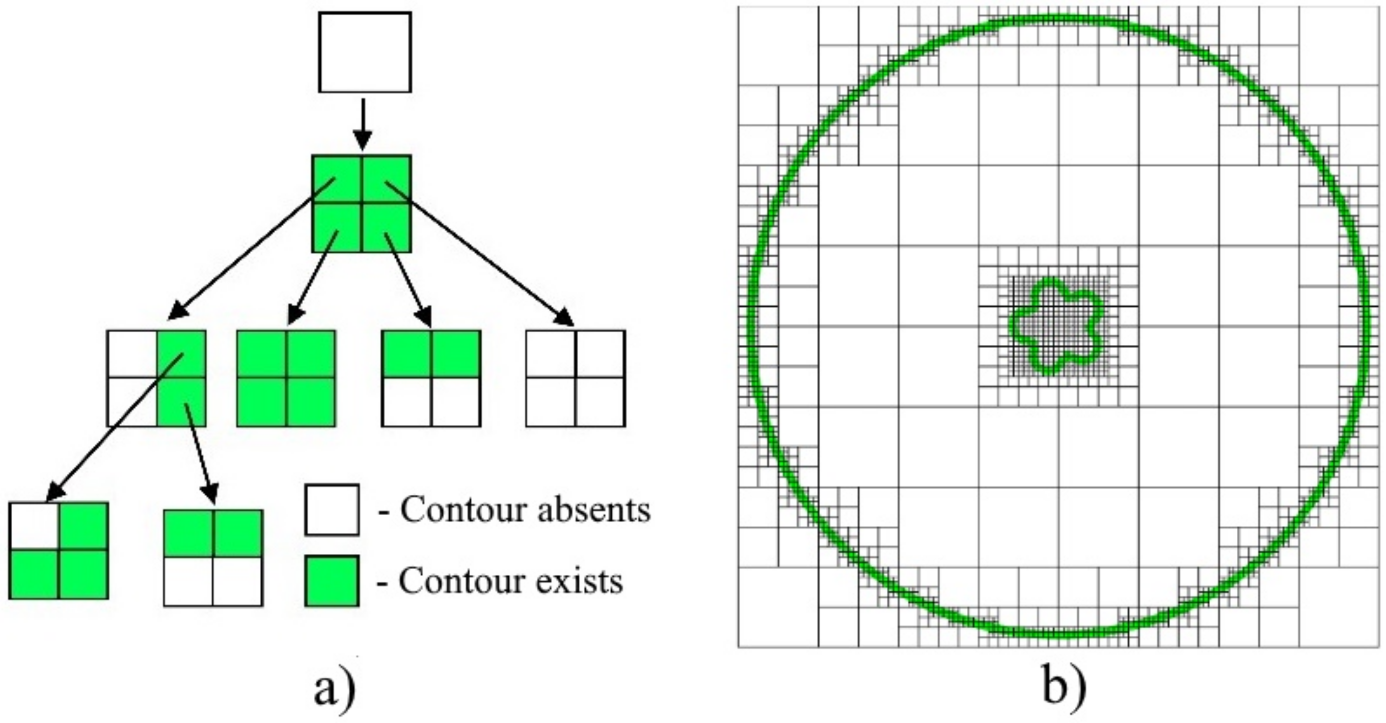
The slicing process is an essential part of additive manufacturing as well as the direct manufacturing method. The method of direct manufacturing [38] for 3D printing was developed for BRep CAD systems. Moreover, the direct manufacturing algorithm was implemented for row 3D scan data [39]. This method for AM was implemented for FRep in the FRepCAM software [19]. The slicing process obtains 2D contours of the model on each level along the Z-axis (Figure 1). A construction of the 2D contours of a FRep model is localization of the areas where . The typical slicing algorithm for the FRep models consists of the quadtree construction and the marching squares (MS) algorithm [40] with the adaptive criteria. The MS algorithm is used to construct the contour topology, quadtrees and adaptive criteria are used to speed up calculations.
The quadtree is built from the root node, which is the bounding box of the implicit curve. Then, it is divided into four equal regions, which form the child nodes. Every child node can be recursively divided further. The process of contour extraction using the quadtree for one Z-layer is shown in Figure (Figure 2a). The contouring process requires to calculate the value of the defining function of FRep model at very large number of points. An adaptive subdivision is used for decreasing the number of calculations of the defining function by localize the areas (cells of quadtree) which contains implicit curve. Adaptive subdivision can employ an interval [41,42] or affine arithmetic [17] as common adaptive criteria [16], which allows you to evaluate the upper and lower bounds of the range of values of the defining function for each cell of the quadtree and decide whether to split the cell or not. In interval arithmetic, every quantity is represented by an interval of real numbers. An interval is a set of such that . During functions processing in interval arithmetic, each quantity is replaced by its interval extension, and all computations are executed on intervals. If the upper and lower bounds of the interval are on opposite sides of zero, this means that the processed quadtree cell contains contours of the curve and should be divided.
In most cases, slicing FRep models constructed using the loop operation is often a computationally complex task. There are two main problems with 2D contour extraction from FRep models equipped with the loop operation. The first problem is that common adaptive criteria (interval, affine or revised affine arithmetic) do not work properly with such models due to interval overestimations. The intervals of values of the defining function becomes wide, and the algorithm divides all the cells of the quadtree without adaptivity. The second problem is the slow performance of the loop operation.
The proposed solution to both problems is to use an acceleration method based on the spatial indexes. We present the accelerated slicing algorithm, which uses this technique.
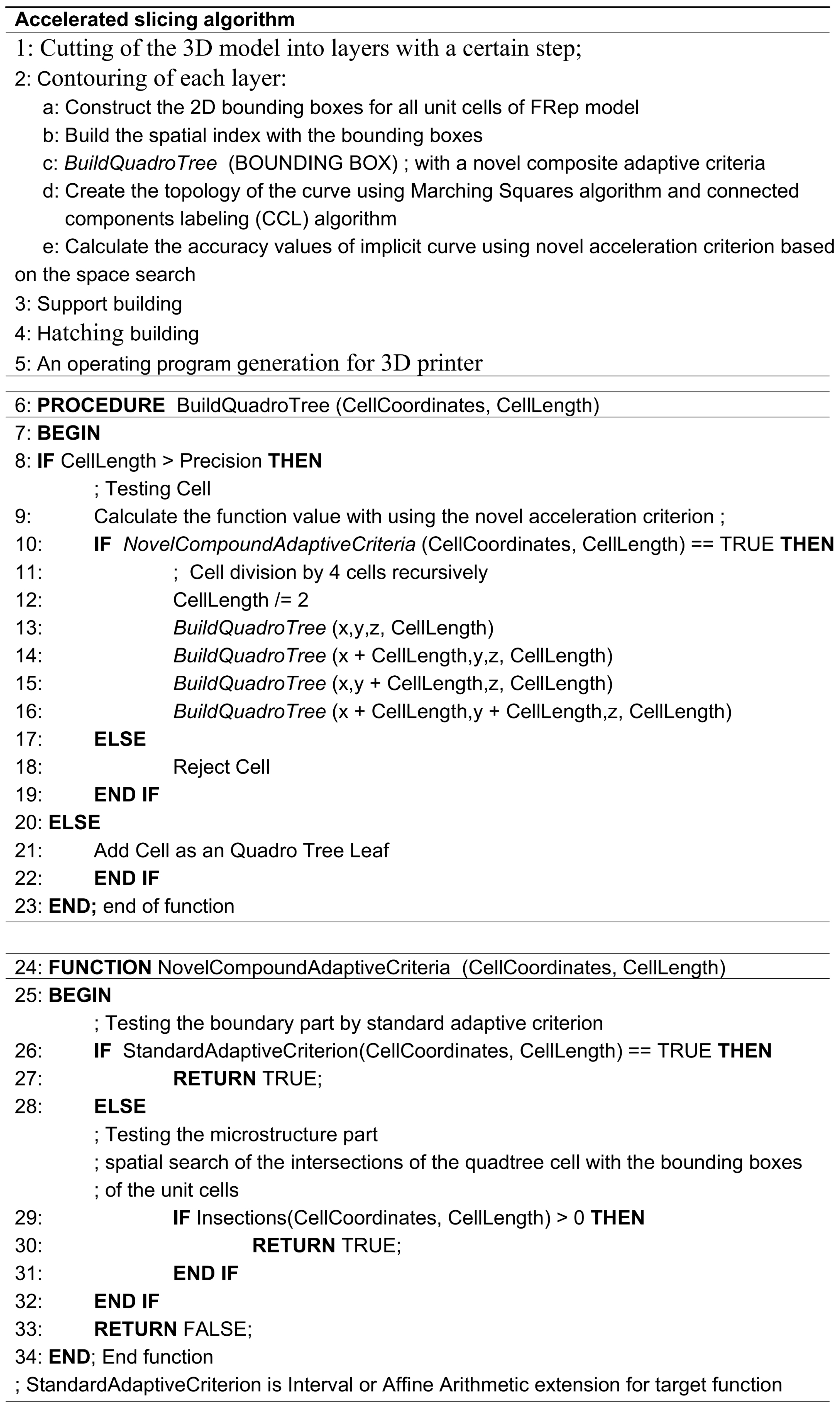
The accelerated slicing algorithm for FRep models satisfying Equation (2) contains the following steps:
- 1.
- Cutting the 3D model into layers with a certain step.
- 2.
- Contouring each layer.
- 3.
- Post-processing the obtained contours with support and hatching building.
- 4.
- Generating the operating program for a certain 3D printer.
An acceleration of the proposed slicing algorithm is reached by applying the specific contouring algorithm, which consists of the following steps:
- 1.
- Constructing the 2D bounding boxes for all the unit cells of the FRep model (Figure 3a red rectangles).
- 2.
- Building the spatial index structure with the precalculated bounding boxes of the unit cells in each layer of the sliced 3D model (Figure 3).
- 3.
- Applying the novel compound adaptive criterion based on the spatial query during quadtree construction for the FRep model (Figure 2a).
- 4.
- Applying the novel acceleration criterion based on the spatial search during calculating the defining function at every point of interest in the space.
- 5.
- Creating the topology of the curve using the MS algorithm and the connected component labelling (CCL) algorithm [43].
- 6.
- Calculating the exact values of the implicit curve on the edges of adjacent cells using numerical methods for solving nonlinear equations.
The detailed pseudocode of the algorithm is shown in Figure 4.
The detailed description of the novel compound adaptive criterion and the novel acceleration criterion will be given in the next sections. The CCL algorithm was implemented according to [43]. The simple bisection method is used for solving the nonlinear equation (the defining function of the FRep model in the contouring process). These steps of the algorithm are implemented in FRepCAM [19].
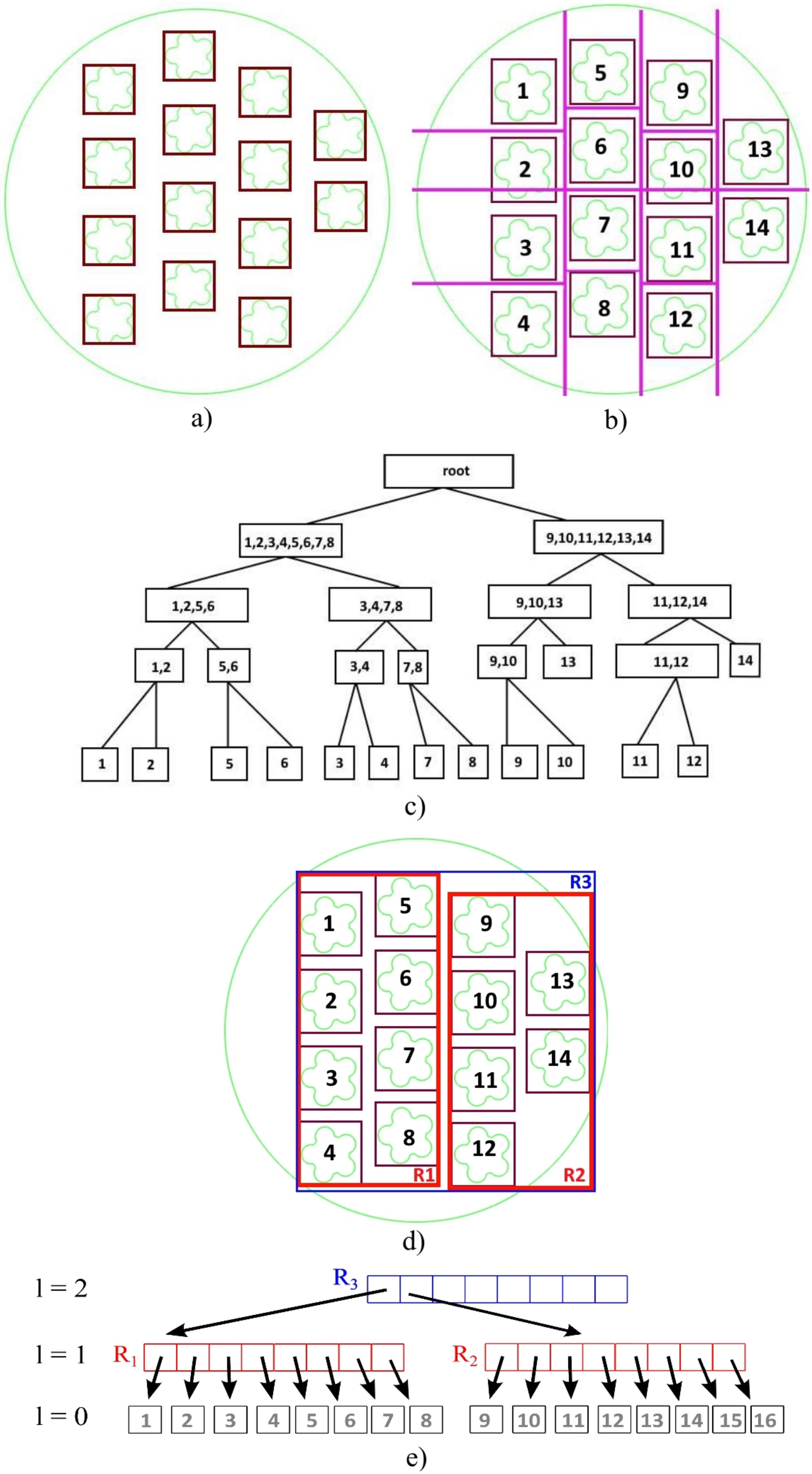
The process of constructing the spatial index (K-d tree) with 2D rectangles is shown in Figure 3b,c. The median thresholding strategy is used for the space division by a splitting plane. Every construction step divides the space at the median point of the arranged bounding boxes by X- and Y-aligned planes alternately. Unit cells on the left side of the median point are stored in the left subtree, and those on the right side of the median point are stored in the right subtree. The process stops after all the unit cells have been arranged or the width of the box of the leaf node is minimized. Every leaf of the K-d tree stores only one unit cell.
Instead of a K-d tree, an R-tree can also be used as the spatial index Figure 3d,e. There are linear and quadratic R-tree creation algorithms. The quadratic algorithm splits an overflow node by the two nodes with a minimal area of bounding boxes. The linear algorithm uses a splitting strategy based on the maximal distance between bounding boxes. We used the quadric R-tree creation algorithm, where the maximal number of elements in the node equals 8 and minimal number of elements in the node equals 2. This algorithm was chosen because of the simplicity of its implementation and the availability of non-commercial libraries with this algorithm. Additionally, hierarchical structures such as bounding volume hierarchies (BVHs) [26] can be used as the spatial index.
The postprocessing of the contours with the 3D printer operating program generation was performed in FRepCAM.
3.1. Novel Compound Adaptive Criterion
Application of the common adaptive criteria for slicing of FRep models with the loop operations faces the problem of the overestimation of the intervals [18]. It leads to the processing of almost all the quadtree cells in the space. In this case the adaptive contouring approach becomes the exhaustive enumeration method (Figure 5a). In the accelerated slicing algorithm during the quadtree construction process, the decision of dividing each cell of the quadtree is made based on the novel compound adaptive criterion.
Let us divide the initial FRep model by the boundary part and the microstructure part consisted of unit cell repetition. The novel compound adaptive criterion consists of the common adaptive criterion for the boundary of the 3D model (interval or affine arithmetic) and the spatial queries, which are applied to the microstructure. It works as an adaptive criterion for each quadtree cell in the following way: if the interrogated quadtree cell contains at least one bounding box of the microstructure unit cell, this criterion returns true; The spatial query (intersection of the bounding boxes) is used for verification. Thus, the novel compound adaptive criterion obtains its value from the common adaptive criteria for the boundary of the 3D model and from the intersection operation with the spatial search. If at least one of these two conditions is true, the quadtree cell is divided for further computations.
The novel compound adaptive criterion optimizes calculation of the FRep defining function. It reduces the number of processed cells as shown in (Figure 5b). More details about the efficiency of the novel compound adaptive criterion are shown in Case study 1.
3.2. Novel Acceleration Criterion
Applying the spatial search solves the performance problem for the loop operation by reducing the number of iterations. It allows for the evaluation only of a part of an FRep model.
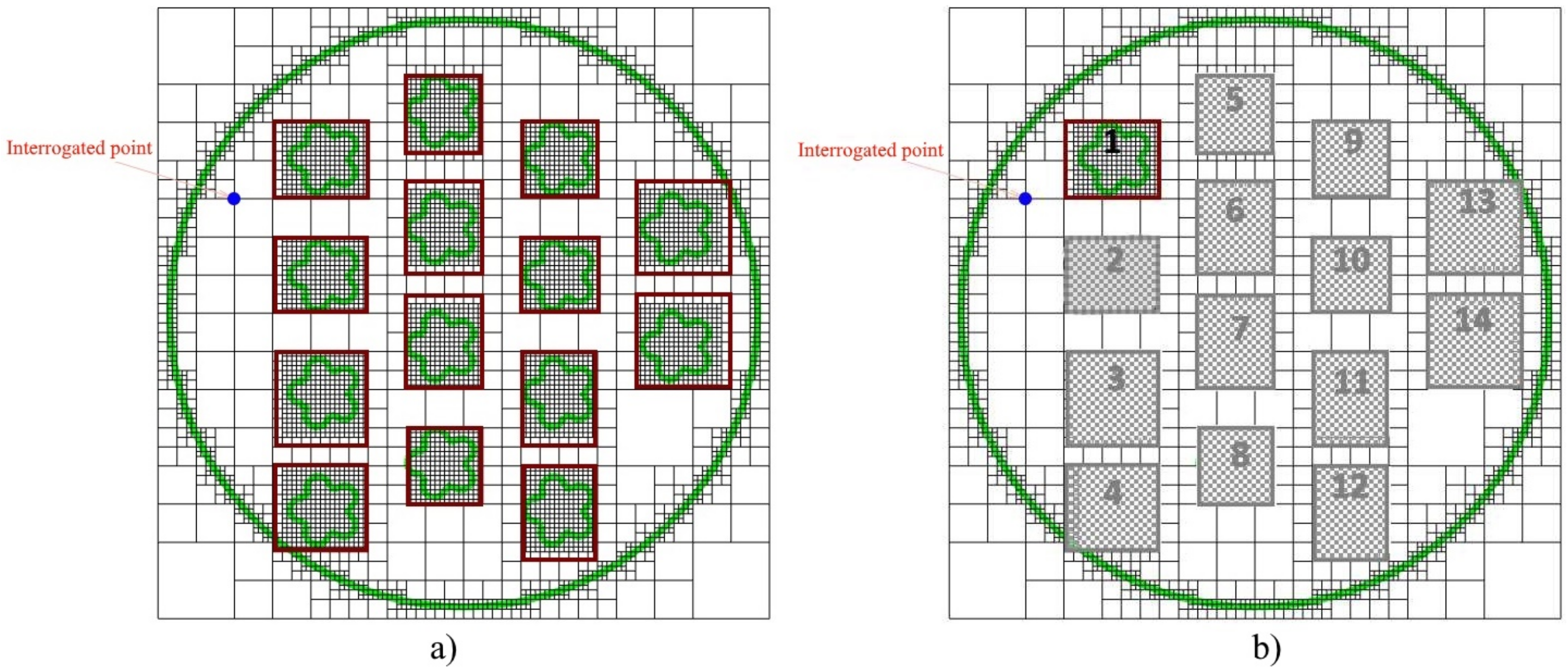
The distance field calculation at every point of interest in the space leads to the computation of all the loop operations to build all the parts of the microstructure. It performs, even if these parts are very far from the point of interest and do not influence its distance field value (Figure 6a). Applying the spatial index allows for processing of only the unit cell closest to the point of interest. The Euclidean distance to the bounding box is used to find the nearest unit cell. Thus, the loop operation is replaced by a spatial search of the unit cell closest to the contours construction. During the calculation of the defining function of the FRep model, only the nearest unit cell (channel number 1 in Figure 6b) is taken into account for the computation, replacing the loop operation.
The computational complexity of the search of the nearest elements to the point of interest is close to O (log n) using a spatial index, in contrast to performing the full loop operation with complexity O . The spatial index based on the K-d tree or R-tree is constructed for every layer of the sliced 3D model and is used to calculate the distance field value for 2D contour construction. It should be noted that the performance can be further improved by applying interval or affine arithmetic to the found unit cells.
Using this criterion makes the defining function of the FRep model discontinuous. It does not affect the contouring process, but the obtained model cannot be used as a primitive in further modelling process. This means that this criterion has to be applied at the end of the modelling process.
The accelerated slicing algorithm was implemented using C++17 and incorporated into the FRepCAM system. The template-based Boost library was used for R-tree construction with the quadric creation algorithm [44]. ALGLIB 3.16.0 was used to construct the K-d tree with the median thresholding strategy for space division [45].
Two examples of the application of the accelerated slicing algorithm will be given in the following sections. The tests for these case studies were performed using the following hardware: a PC with Intel Core i5-8250U CPU @ 1.80 GHz and 8 GB RAM.
4. Results
4.1. Case Study 1: Slicing of a Filter Model
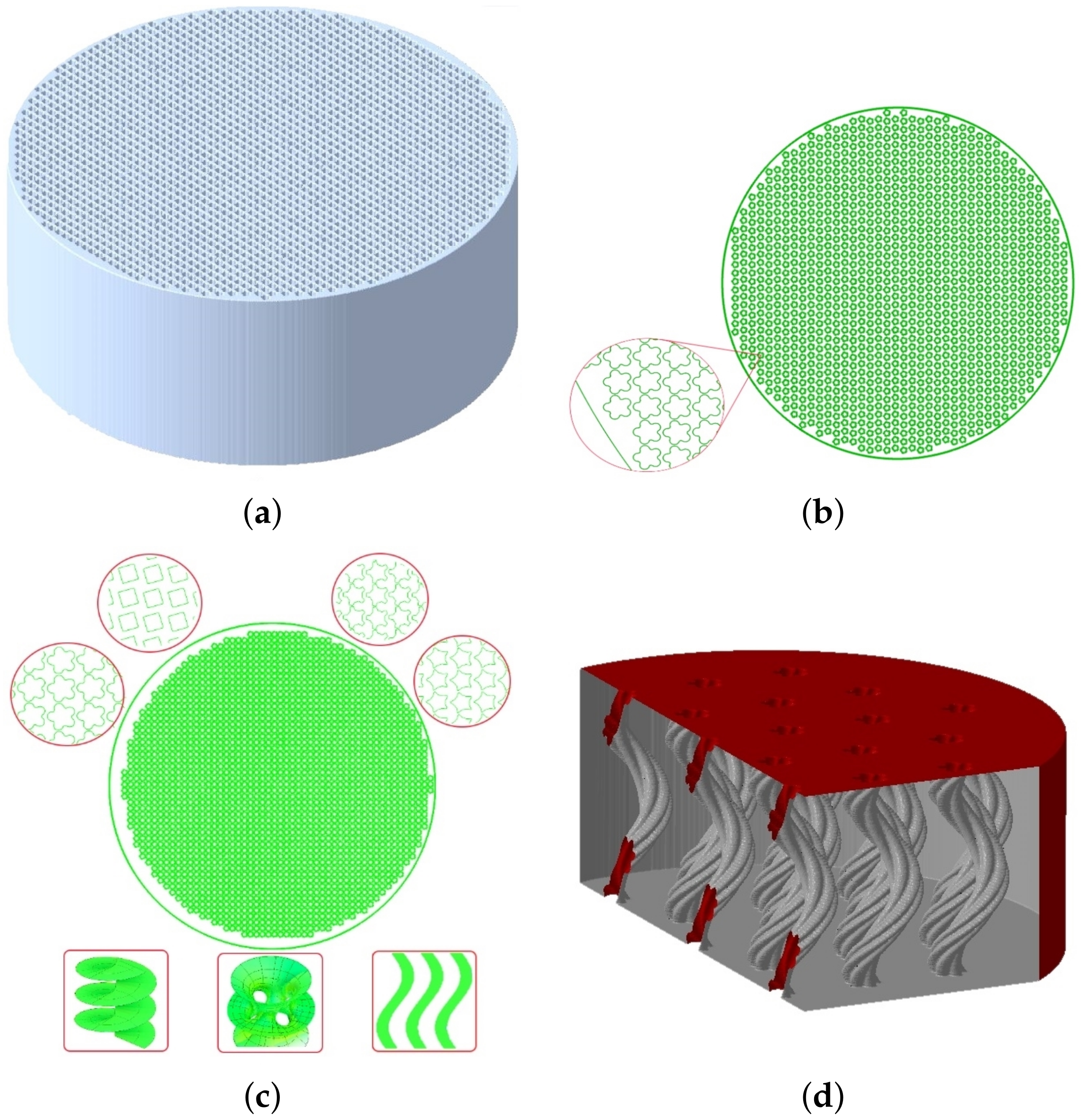
The first studied model was a filter for natural gas separation (Figure 7). This model could be used in optimization tasks, where the new geometry of the filter could be obtained by changing its parameters (Figure 7c). The reason for using the loop operation in the filter model was the complicated topology of its channels. Every channel should be placed in a specific area and rotated at different angles to reach the required density of the channels and the porosity of the whole filter. When the diameter of the channels was very tiny, the number of them increased dramatically. This phenomenon led to an increase in the slicing time. The unit cell in this model was one channel. Different shapes of one channel are shown in Figure 8.
The filter model had 13 parameters: the filter height; filter radius; channel radius; N-pointed star channel; maximal angle channel rotation; distance between channels; thickness shell; shift of the channel from the center; maximal number of channels; type filling for the channels; shape of the channel entry hole; and the shape of the channel Z line.
The unit cell function defines one channel of the filter FRep model. It is built from the profile function . The set of used profiles is shown in Figure 9. The simplest circle shape (Figure 9a) is defined by
The result has the following form
where the space mapping is defined by one of the following equations. For a sinusoidal mapping, it is
For a twisting mapping, it is
For a zigzag mapping, it is
In all the above-mentioned equations
where and are the bottom and top z coordinates of a channel, respectively; and are the rotation angles at the end points; is the amplitude of the space mapping.
The operator of unit cell replication is
where and are the centers of the channels in the loop operation and denotes the set-theoretic union.
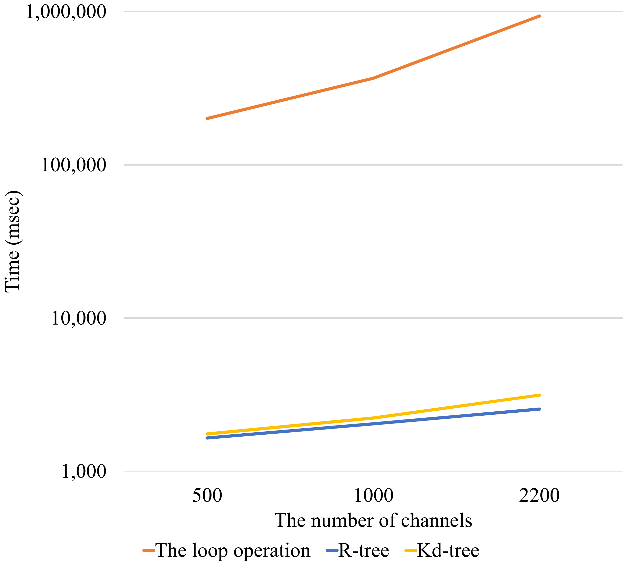
The application of the new slicing algorithm to the filter model with 2200 unit cells allows the reduction in the number of processed cells by 30% due to the novel compound adaptive criterion (Table 1). The contouring time was sped up 100-fold due to using the novel compound adaptive criterion with the novel acceleration criterion (Table 2).
The tests were conducted 20 times for each filter model with different parameters (Table 3) with an XY-resolution of 0.05 mm. The average values were calculated. The results of contouring the one layer of the filter model with a different number of channels and different shapes of the channel’s entry holes are presented in Table 1 and Table 2 and Figure 10. It should be noted that the shape of the channels (sinusoidal, twisting, zigzag) almost did not affect the slicing time.
The Table 2 with the experimental results shows that the use of spatial indexes significantly reduces the slicing time. At the same time, the R-tree and K-d tree data structures show almost the same performance. The shape of the channel entry hole affected the slicing time due to additional calculations of the channel shape.
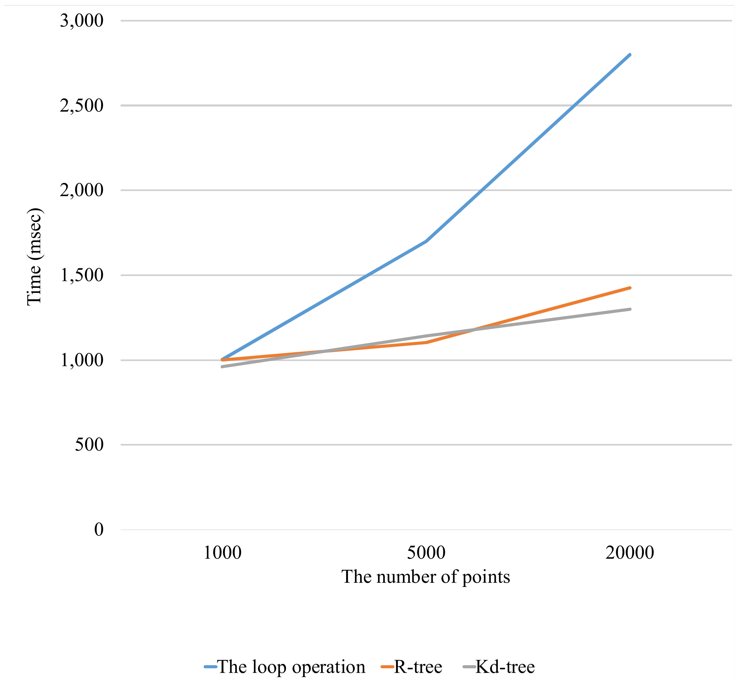
4.2. Case Study 2: Slicing of a Free-Form Model
A free-form model is an FRep model with the following defining function:
where are real number coefficients and are basis functions. In general, can be any continuous functions from some predefined class. In the considered example, we used bilinear spline functions. Computing the defining function is performed with the loop operation and depends on the number of the basis functions. The number of basis functions increases with the accuracy or the number of dimensions of the model together with the computational complexity. The proposed slicing algorithm is applied to with local support. It reduces the number of calculations of the basis functions in the FRep defining function computation. The set of calculated basis functions is limited by four nearest neighbour basis functions around the point of interest.
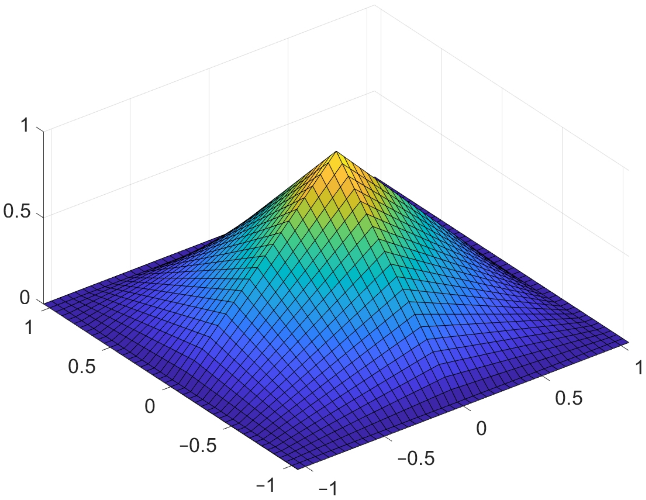
To construct the bilinear spline, the following function is used (Figure 11):
The free-form object consists of following basis functions:
The parameters and define the center of the support of , and define dimensions of the rectangular area the function affects. This area can be written as . Therefore, the defining function of the considered free-form object is
For this FRep model the following function exists:
This function , where is a set of intervals in R, returns the bounding boxes which are quarters of the supports of the basis function .
The unit function for the bounding box is:
where are basis functions with the supports that include . There can be one to four functions in the sum.
5. Discussion and Conclusions
Loop operations are often required for the 3D FRep modelling of complex forms using the unit cell replication. K-d trees and R-trees can be effectively used as acceleration data structures in slicing processes for 3D printing of such FRep models. The accelerated slicing algorithm was proposed, which is based on a novel compound adaptive criterion and a novel acceleration criterion. It reduces the number of processed cells during adaptive contouring and replaces the loop operation by a spatial search.
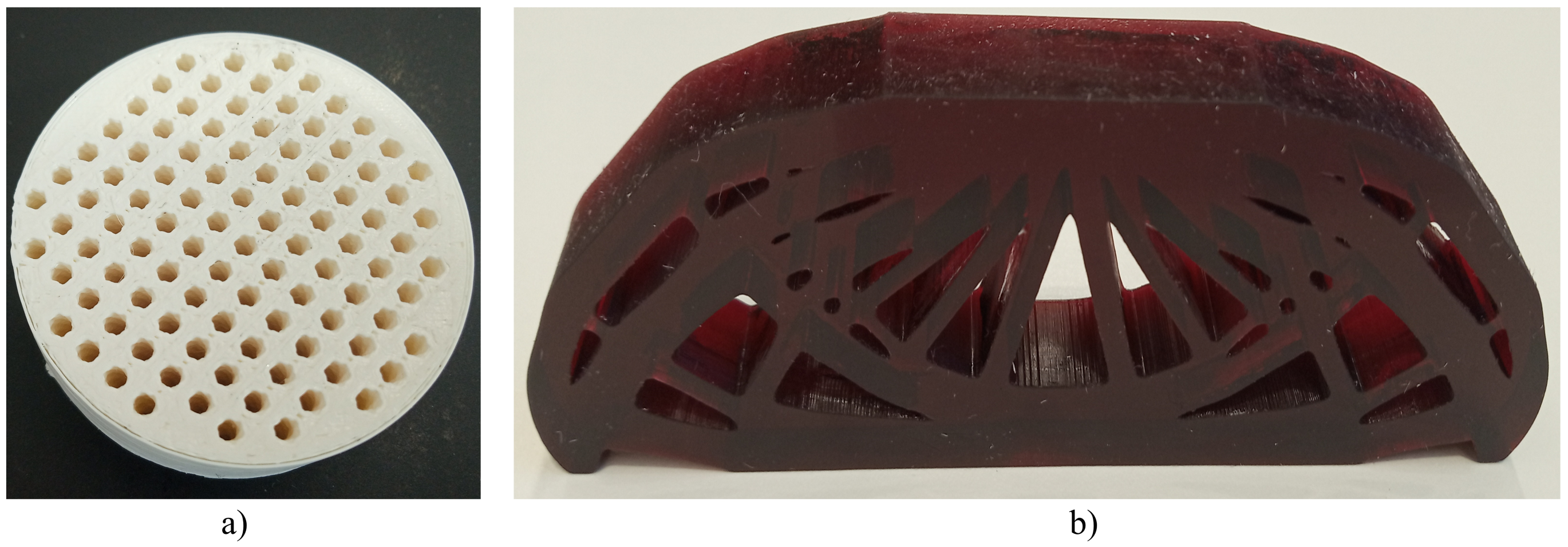
Computational tests of the new slicing algorithm were conducted for two examples of FRep models with complex geometries. It shows 30% reduction in the number of processed cells for the filter model; 100 times reduction in the contouring time for the filter model and 2 times reduction in the contouring time for the free-form model accordingly. The median threshold strategy of a space division was used for the K-d tree construction. The quadratic algorithm was employed for the R-tree construction. The R-tree application to the filter model shows a bit higher performance compared to K-d tree construction due to use of the spatial query for the search of intersections between the bounding boxes of the unit cells. Generally, the experimental results show equal performance for R-tree and K-d tree. The computation complexity of the contouring process using the novel accelerated slicing algorithm becomes O in contrast to O. The accelerated slicing algorithm was incorporated into the system of additive manufacturing for FRep modelling (FRepCAM). This system uses the direct manufacturing approach, which allows for printing FRep models directly without creating an intermediate STL file. The slicing algorithm significantly reduces the time needed to contour FRep models during 3D printing preparation. Both models (Figure 7 and Figure 12) were sliced with FRepCAM and fabricated. An Ultimaker S5 FDM 3D printer was used to construct the filter model (Figure 14a, radius 25 mm, height 20 mm). A Wanhao Duplicator 7 DLP 3D printer was used to construct the free-form FRep model (Figure 14b, length 100 mm, width 50 mm, height 20 mm).
Author Contributions
Conceptualization, E.M., D.P. and A.P.; Writing—original draft, E.M. and D.P.; Writing—review and editing, S.C., A.P. and I.A. All authors have read and agreed to the published version of the manuscript.
Funding
This research received no external funding.
Institutional Review Board Statement
Not applicable.
Informed Consent Statement
Not applicable.
Conflicts of Interest
The authors declare no conflict of interest.
References
- Roscoe, L. Stereolithography interface specification. In Stereolithography Interface Specification; 3D Systems Inc.: Valencia, CA, USA, 1988. [Google Scholar]
- Burns, M. Automated Fabrication: Improving Productivity in Manufacturing; PTR Prentice Hall: Englewood Cliffs, NJ, USA, 1993. [Google Scholar]
- 3MF-Consortium. 3Mf Format Specification; 3MF-Consortium: Wakefield, MA, USA, 2020. [Google Scholar]
- Pasko, A.; Adzhiev, V.; Sourin, A.; Savchenko, V. Function representation in geometric modeling: Concepts, implementation and applications. Vis. Comput. 1995, 11, 429–446. [Google Scholar] [CrossRef]
- Steuben, J.C.; Iliopoulos, A.P.; Michopoulos, J.G. Implicit slicing for functionally tailored additive manufacturing. Comput. Aided Des. 2016, 77, 107–119. [Google Scholar] [CrossRef]
- Chen, M.; Tucker, J.V. Constructive Volume Geometry. Comput. Graph. Forum 2000, 19, 281–293. [Google Scholar] [CrossRef] [Green Version]
- Rvachev, V.L. Theory of R-Functions and Some Applications; Naukova Dumka: Kyiv, Ukraine, 1982. [Google Scholar]
- Pasko, A.; Fryazinov, O.; Vilbrandt, T.; Fayolle, P.; Adzhiev, V. Procedural function-based modelling of volumetric microstructures. Graph. Model. 2011, 73, 165–181. [Google Scholar] [CrossRef] [Green Version]
- Schwarz, H. Gesammelte Mathematische Abhandlungen; Springer: Berlin/Heidelberg, Germany, 1890. [Google Scholar] [CrossRef] [Green Version]
- Pasko, G.; Pasko, A.; Ikeda, M.; Kunii, T. Bounded blending operations. In Proceedings of the SMI Shape Modeling International 2002, Banff, AB, Canada, 17–22 May 2002; pp. 95–103. [Google Scholar] [CrossRef]
- Safonov, A.; Maltsev, E.; Chugunov, S.; Tikhonov, A.; Konev, S.; Evlashin, S.; Popov, D.; Pasko, A.; Akhatov, I. Design and Fabrication of Complex-Shaped Ceramic Bone Implants via 3D Printing Based on Laser Stereolithography. Appl. Sci. 2020, 10, 7138. [Google Scholar] [CrossRef]
- Sanchez, M.; Fryazinov, O.; Fayolle, P.; Pasko, A. Convolution Filtering of Continuous Signed Distance Fields for Polygonal Meshes. Comput. Graph. Forum 2015, 34, 277–288. [Google Scholar] [CrossRef] [Green Version]
- Weisstein, E.W. Sawtooth Wave. In MathWorld—A Wolfram Web Resource. 2010. Available online: https://mathworld.wolfram.com/SawtoothWave.html (accessed on 5 March 2021).
- Weisstein, E.W. Triangle Wave. In MathWorld—A Wolfram Web Resource. 2010. Available online: https://mathworld.wolfram.com/TriangleWave.html (accessed on 5 March 2021).
- Fryazinov, O.; Vilbrandt, T.; Pasko, A. Multi-scale space-variant FRep cellular structures. Comput. Aided Des. 2013, 45, 26–34. [Google Scholar] [CrossRef] [Green Version]
- Stolte, N.; Kaufman, A. Parallel Spatial Enumeration of Implicit Surfaces using Interval Arithmetic for Octree Generation and its direct Visualization. In Proceedings of the Implicit Surfaces’98, Seattle, WA, USA, 15–16 June 1998; pp. 81–87. [Google Scholar]
- Stolfi, J.; De Figueiredo, L. An introduction to affine arithmetic. Trends Appl. Comput. Math. 2003, 4, 297–312. [Google Scholar] [CrossRef]
- Fryazinov, O.; Pasko, A.; Comninos, P. Fast Reliable Interrogation of Procedurally Defined Implicit Surfaces Using Extended Revised Affine Arithmetic. Comput. Graph. 2010, 34, 708–718. [Google Scholar] [CrossRef] [Green Version]
- Popov, D.; Maltsev, E.; Fryazinov, O.; Pasko, A.; Akhatov, I. Efficient contouring of functionally represented objects for additive manufacturing. Comput. Aided Des. 2020. [Google Scholar] [CrossRef]
- Bühler, K. Implicit linear interval estimations. In Proceedings of the 18th Spring Conference on Computer Graphics, Budmerice, Slovakia, 24–27 April 2002; pp. 123–132. [Google Scholar] [CrossRef]
- Havran, V.; Bittner, J. On Improving KD-Trees for Ray Shooting. In Proceedings of the WSCG 2002 Conference, Plzen-Bory, Czech Republic, 4–8 February 2002; pp. 209–217. [Google Scholar]
- Foley, T.; Sugerman, J. KD-Tree Acceleration Structures for a GPU Raytracer. In Proceedings of the ACM SIGGRAPH/EUROGRAPHICS Conference on Graphics Hardware, Los Angeles, CA, USA, 30–31 July 2005; pp. 15–22. [Google Scholar] [CrossRef]
- Wen, P.; Xiaojun, W.; Gao, T.; Wu, C. Kd-Tree Based OLS in Implicit Surface Reconstruction with Radial Basis Function. In Proceedings of the International Conference on Artificial Reality and Telexistence: Advances in Artificial Reality and Tele-Existence, Hangzhou, China, 29 November–1 December 2006; Volume 4282, pp. 861–870. [Google Scholar] [CrossRef]
- Feldmann, D. Accelerated ray tracing using R-trees. In Proceedings of the GRAPP 2015–10th International Conference on Computer Graphics Theory and Applications, Berlin, Germany, 11–14 March 2015; pp. 247–257. [Google Scholar]
- Wang, L.; Yu, Y.; Zhou, K.; Guo, B. Multiscale Vector Volumes. ACM Trans. Graph. 2011, 30, 1–8. [Google Scholar] [CrossRef]
- Gourmel, O.; Pajot, A.; Paulin, M.; Barthe, L.; Poulin, P. Fitted BVH for Fast Raytracing of Metaballs. Comput. Graph. Forum 2010, 29. [Google Scholar] [CrossRef] [Green Version]
- Bentley, J. Multidimensional Binary Search Trees Used for Associative Searching. Commun. ACM 1975, 18, 509–517. [Google Scholar] [CrossRef]
- MacDonald, J.; Booth, K. Heuristics for ray tracing using space subdivision. Vis. Comput. 1990, 6, 153–166. [Google Scholar] [CrossRef]
- Havran, V. Heuristic Ray Shooting Algorithms. Ph.D. Thesis, Czech Technical University, Prague, Czech Republic, 2000. [Google Scholar]
- Havran, V.; Kopal, T.; Bittner, J.; Zara, J. Fast Robust BSP Tree Traversal Algorithm For Ray Tracing. J. Graph. Tools 1998. [Google Scholar] [CrossRef]
- Guttman, A. R Trees: A Dynamic Index Structure for Spatial Searching. Sigmod Rec. 1984, 14, 47–57. [Google Scholar] [CrossRef]
- Sellis, T. Efficiently supporting procedures in relational database systems. In Proceedings of the 1987 ACM SIGMOD International Conference on Management of Data, San Francisco, CA, USA, 27–29 May 1987; pp. 278–291. [Google Scholar]
- Beckmann, N.; Kriegel, H.; Schneider, R.; Seeger, B. The R*-Tree: An Efficient and Robust Access Method for Points and Rectangles. In Proceedings of the 1990 ACM SIGMOD International Conference on Management of Data, Atlantic City, NJ, USA, 23–26 May 1990; pp. 322–331. [Google Scholar] [CrossRef] [Green Version]
- Beckmann, N.; Seeger, B. A revised R*-tree in comparison with related index structures. In Proceedings of the International Conference on Management of Data, Providence, RI, USA, 29 June–2 July 2009; pp. 799–812. [Google Scholar]
- Finkel, R.; Bentley, J. Quad trees: A data structure for retrieval on composite keys. Acta Inform. 1974, 4, 1–9. [Google Scholar] [CrossRef]
- Klinger, A.; Dyer, C. Experiments on picture representation using regular decomposition. Comput. Graph. Image Process. 1976, 5, 68–105. [Google Scholar] [CrossRef]
- Song, Y.; Yang, Z.; Liu, Y.; Deng, J. Function representation based slicer for 3D printing. Comput. Aided Geom. Des. 2018, 62, 276–293. [Google Scholar] [CrossRef]
- Jamieson, R.; Hacker, H. Direct slicing of CAD models for rapid prototyping. Rapid Prototyp. J. 1995, 1, 4–12. [Google Scholar] [CrossRef]
- Chen, Y.; Li, K.; Qian, X. Direct Geometry Processing for Telefabrication. J. Comput. Inf. Sci. Eng. 2013, 13. [Google Scholar] [CrossRef]
- Maple, C. Geometric design and space planning using the marching squares and marching cube algorithms. In Proceedings of the 2003 International Conference on Geometric Modeling and Graphics, London, UK, 16–18 July 2003; pp. 90–95. [Google Scholar] [CrossRef]
- Moore, R. Interval Analysis; Prentice-Hall: Englewood Cliff, NJ, USA, 1966. [Google Scholar]
- Sunaga, T. Theory of an interval algebra and its application to numerical analysis. Jpn. J. Ind. Appl. Math. 2009, 26, 125–143. [Google Scholar] [CrossRef]
- Shapiro, L. Connected Component Labeling and Adjacency Graph Construction. Mach. Intell. Pattern Recognit. 1996, 19, 1–30. [Google Scholar] [CrossRef]
- Gehrels, B.; Lalande, B.; Loskot, M.; Wulkiewicz, A. Boost Library. 2009. Available online: https://www.boost.org/ (accessed on 5 March 2021).
- ALGLIB-Project. Data Processing Library; ALGLIB-Project: Nizhny Novgorod, Russia, 1999. [Google Scholar]
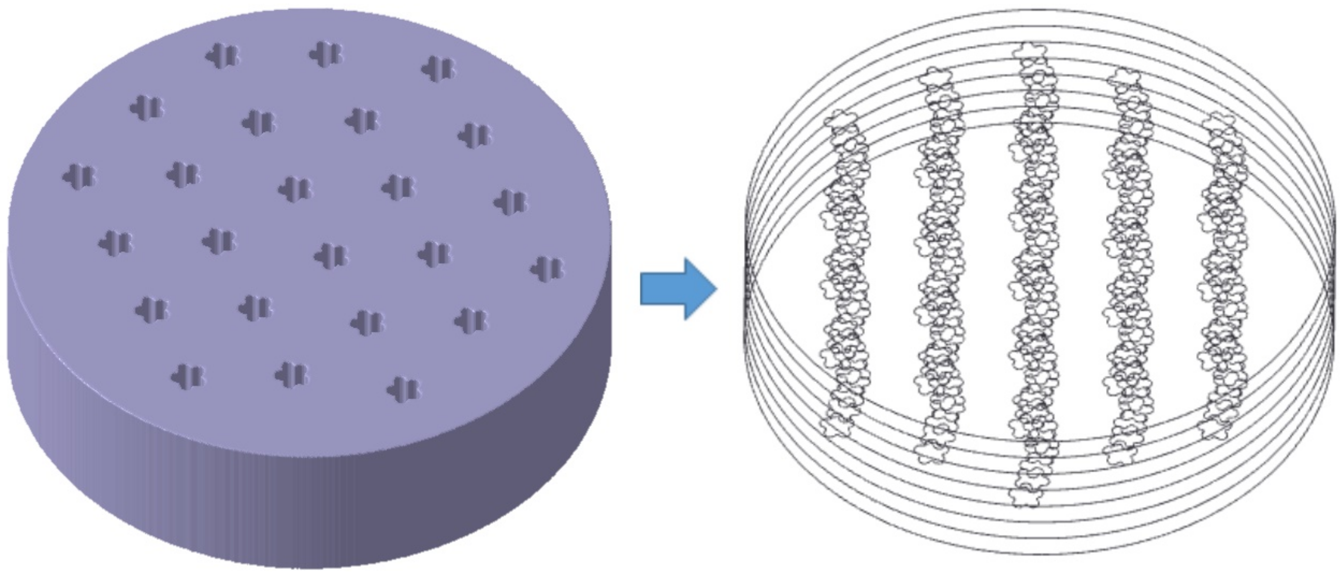
Figure 1.
Slicing of the FRep model allows obtaining 2D contours within each layer along the Z-axis.
Figure 1.
Slicing of the FRep model allows obtaining 2D contours within each layer along the Z-axis.

Figure 2.
The contour extraction process for one layer of the FRep model: (a) building a quadtree, (b) contouring of one layer using the quadtree.
Figure 2.
The contour extraction process for one layer of the FRep model: (a) building a quadtree, (b) contouring of one layer using the quadtree.

Figure 3.
The process of K-d tree and R-tree construction for one layer of the FRep model: (a) bounding boxes of the unit cells (green lines—extracted contours, red rectangles—bounding boxes), (b) K-d tree construction, division of the space (purple lines), (c) K-d tree, (d) R-tree construction (max. number of elements in the node = 8 and min. number of elements in the node = 2), (e) R-tree.

Figure 4.
An accelerated slicing algorithm for an FRep model.

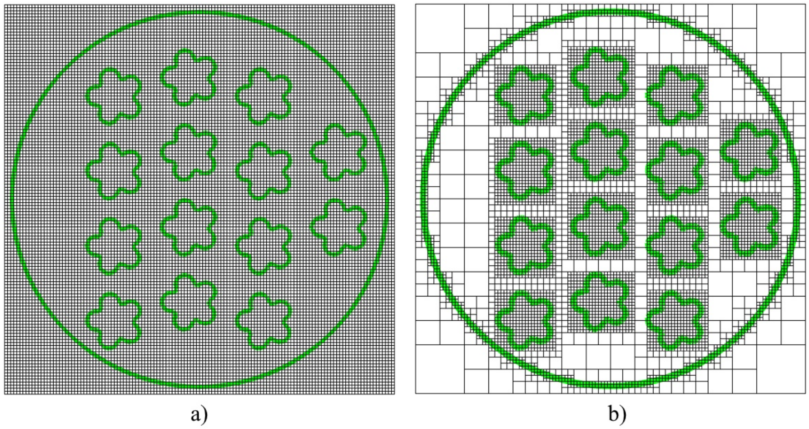
Figure 5.
The contour extraction of one layer of the FRep model (contours—green lines, quadtree cells—black lines): (a) using a common adaptive criterion (b) using the novel compound adaptive criterion.
Figure 5.
The contour extraction of one layer of the FRep model (contours—green lines, quadtree cells—black lines): (a) using a common adaptive criterion (b) using the novel compound adaptive criterion.

Figure 6.
The process of contour extraction in one layer of the FRep model: (a) the full loop operation (b) the novel compound adaptive and acceleration criteria. (green lines—extracted contours, black lines—quadtree structure, red rectangles—precalculated bounded boxes of each channel of microstructure, blue point—point of interest).

Figure 7.
The filter model with channels: (a) the 3D object of the filter model; (b) cross-section of the 3D model with zoom; (c) Cross-sections of the filter model with parameterization examples; (d) the 3D object of the filter model with an X-Y cross-section.
Figure 7.
The filter model with channels: (a) the 3D object of the filter model; (b) cross-section of the 3D model with zoom; (c) Cross-sections of the filter model with parameterization examples; (d) the 3D object of the filter model with an X-Y cross-section.

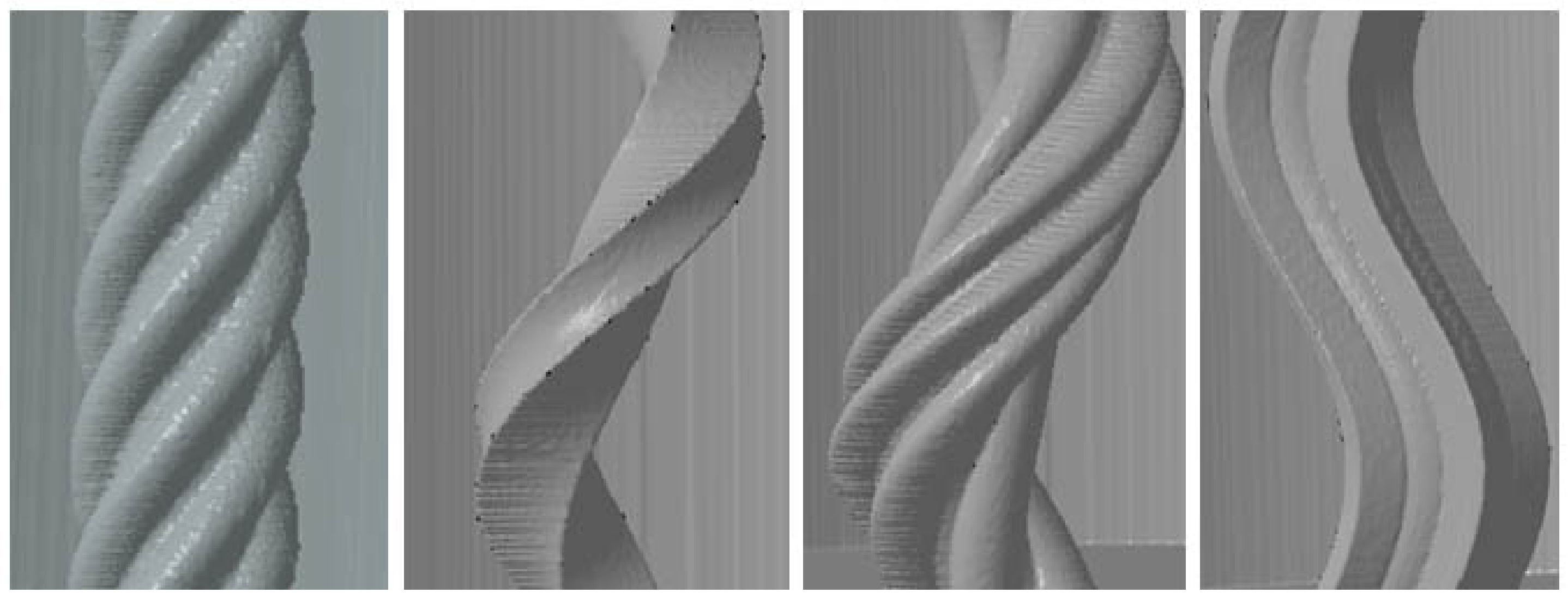
Figure 8.
Different shapes of channels.

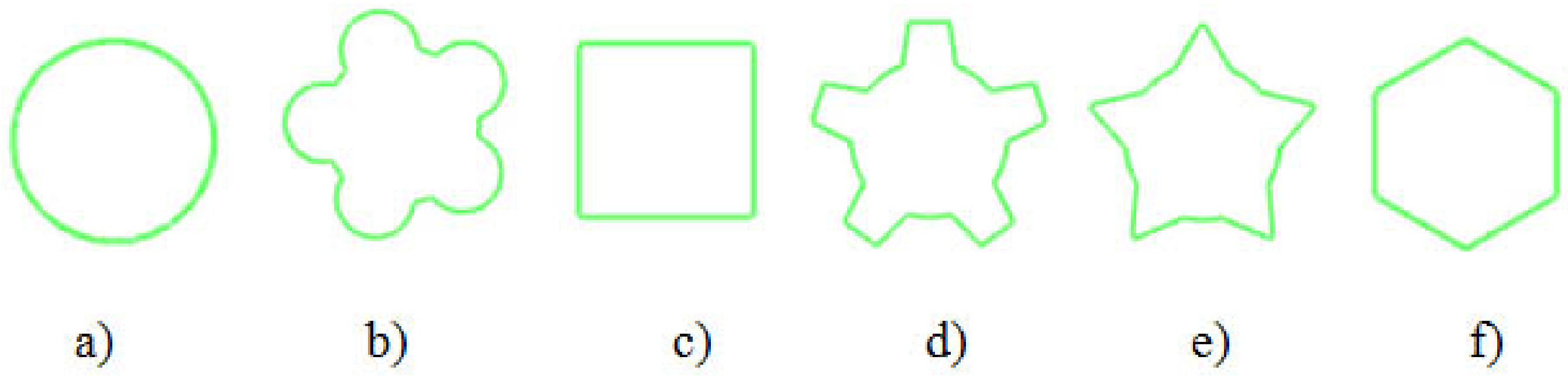
Figure 9.
The shapes of the entry holes: (a) circle, (b) circle with petals, (c) square, (d) gear, (e) star, (f) hexagon.
Figure 9.
The shapes of the entry holes: (a) circle, (b) circle with petals, (c) square, (d) gear, (e) star, (f) hexagon.

Figure 10.
Plot of the experimental results with the filter model (the shape of the channel’s entry holes: a circle with petals).
Figure 10.
Plot of the experimental results with the filter model (the shape of the channel’s entry holes: a circle with petals).

Figure 11.
Plot of .

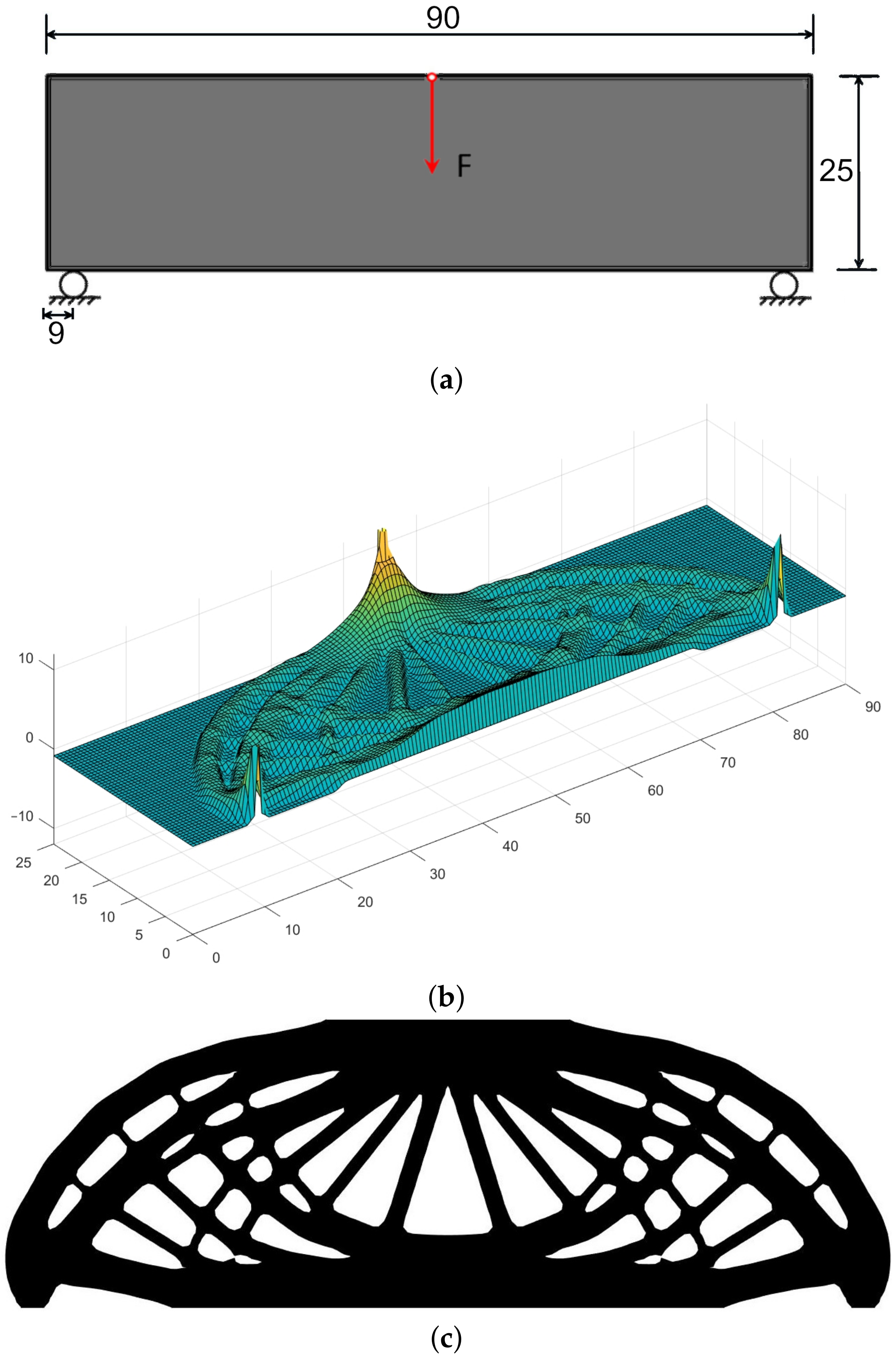
Figure 12.
An example of a free-form model obtained via topology optimization algorithm: (a) boundary conditions of the topology optimization task for compliance minimization, (b) the plot for the obtained free-form function and (c) the optimized shape defined by the free-form function .
Figure 12.
An example of a free-form model obtained via topology optimization algorithm: (a) boundary conditions of the topology optimization task for compliance minimization, (b) the plot for the obtained free-form function and (c) the optimized shape defined by the free-form function .

Figure 13.
Plot of the experimental results with the free-form model.

Figure 14.
Printed models: the filter model printed using an Ultimaker S5 3D FDM printer (a), the free-form FRep model printed using a Wanhao Duplicator 7 DLP 3D printer (b).
Figure 14.
Printed models: the filter model printed using an Ultimaker S5 3D FDM printer (a), the free-form FRep model printed using a Wanhao Duplicator 7 DLP 3D printer (b).


Table 1.
The number of processed cells of one layer of the filter model.
| Number of Unit Cells (Channels) | Number of Processed Cells | Reducing % of the Processed Cells | |
|---|---|---|---|
| Common Adaptive Criterion | Novel Compound Adaptive Criterion | ||
| 500 | 362,479 | 244,989 | 33 |
| 1000 | 362,479 | 249,269 | 32 |
| 2200 | 362,479 | 250,129 | 31 |
Table 2.
Experimental results of the filter model slicing step.
| Channel Diameter (mm) | Number of Channels | Slicing Time (ms) | ||
|---|---|---|---|---|
| Slicing with the Full Loop Operation | Accelerated Slicing Algorithm | |||
| R-Tree | K-d Tree | |||
| circle | ||||
| 1.8 | 500 | 63,552 | 1273 | 1222 |
| 1.5 | 1000 | 99,944 | 1351 | 1310 |
| 0.9 | 2200 | 297,326 | 1683 | 1779 |
| circle with petals | ||||
| 1.8 | 500 | 200,530 | 1651 | 1754 |
| 1.5 | 1000 | 367,219 | 2042 | 2230 |
| 0.9 | 2200 | 936,803 | 2550 | 3145 |
| square | ||||
| 1.8 | 500 | 82,073 | 1432 | 1875 |
| 1.5 | 1000 | 124,205 | 1550 | 2107 |
| 0.9 | 2200 | 390,451 | 1970 | 2584 |
| gear | ||||
| 1.8 | 500 | 1,063,341 | 2794 | 3328 |
| 1.5 | 1000 | 1,947,765 | 3001 | 3719 |
| 0.9 | 2200 | 4,454,432 | 4214 | 5205 |
| star | ||||
| 1.8 | 500 | 1,076,432 | 2487 | 2957 |
| 1.5 | 1000 | 1,971,207 | 2703 | 3436 |
| 0.9 | 2200 | 4,509,271 | 3738 | 4411 |
| hexagon | ||||
| 1.8 | 500 | 129,222 | 1436 | 1906 |
| 1.5 | 1000 | 214,078 | 1698 | 2147 |
| 0.9 | 2200 | 634,755 | 2008 | 2591 |
Table 3.
The filter model parameters.
| Parameter | Value |
|---|---|
| Height of the filter | 20 mm |
| Diameter of the filter | 50 mm |
| Channel diameter | 0.9–1.8 mm |
| Number of channels | 500–2200 |
Table 4.
Experimental results for the free-form model.
| Number of Points | Slicing Time (ms) | ||
|---|---|---|---|
| Slicing with the Full Loop Operation | Accelerated Slicing Algorithm | ||
| R-Tree | K-d Tree | ||
| 1250 | 1004 | 1000 | 960 |
| 5000 | 1699 | 1102 | 1143 |
| 20,000 | 2800 | 1425 | 1300 |
Publisher’s Note: MDPI stays neutral with regard to jurisdictional claims in published maps and institutional affiliations. |
© 2021 by the authors. Licensee MDPI, Basel, Switzerland. This article is an open access article distributed under the terms and conditions of the Creative Commons Attribution (CC BY) license (https://creativecommons.org/licenses/by/4.0/).
Share and Cite
MDPI and ACS Style
Maltsev, E.; Popov, D.; Chugunov, S.; Pasko, A.; Akhatov, I. An Accelerated Slicing Algorithm for Frep Models. Appl. Sci. 2021, 11, 6767. https://doi.org/10.3390/app11156767
AMA Style
Maltsev E, Popov D, Chugunov S, Pasko A, Akhatov I. An Accelerated Slicing Algorithm for Frep Models. Applied Sciences. 2021; 11(15):6767. https://doi.org/10.3390/app11156767
Chicago/Turabian StyleMaltsev, Evgenii, Dmitry Popov, Svyatoslav Chugunov, Alexander Pasko, and Iskander Akhatov. 2021. "An Accelerated Slicing Algorithm for Frep Models" Applied Sciences 11, no. 15: 6767. https://doi.org/10.3390/app11156767
Note that from the first issue of 2016, this journal uses article numbers instead of page numbers. See further details here.