
Geometric Deep Lean Learning: Evaluation Using a Twitter Social Network


1
Hochschule Heilbronn, Fakultät Management und Vertrieb, Campus Schwäbisch Hall, 74523 Schwäbisch Hall, Germany
2
Department of Artificial Intelligence, Escuela Técnica Superior de Ingenieros Informáticos, Universidad Politécnica de Madrid, 28660 Boadilla del Monte, Spain
3
Escuela Técnica Superior de Ingenieros Industriales (ETSII), Universidad Politécnica de Madrid, José Gutiérrez Abascal 2, 28006 Madrid, Spain
4
Matthews International GmbH, Gutenbergstraße 1-3, 48691 Vreden, Germany
*
Author to whom correspondence should be addressed.
Appl. Sci. 2021, 11(15), 6777; https://doi.org/10.3390/app11156777
Submission received: 8 June 2021
/
Revised: 21 July 2021
/
Accepted: 22 July 2021
/
Published: 23 July 2021
(This article belongs to the Special Issue Social Network Analysis)
Abstract
:The goal of this work is to evaluate a deep learning algorithm that has been designed to predict the topological evolution of dynamic complex non-Euclidean graphs in discrete–time in which links are labeled with communicative messages. This type of graph can represent, for example, social networks or complex organisations such as the networks associated with Industry 4.0. In this paper, we first introduce the formal geometric deep lean learning algorithm in its essential form. We then propose a methodology to systematically mine the data generated in social media Twitter, which resembles these complex topologies. Finally, we present the evaluation of a geometric deep lean learning algorithm that allows for link prediction within such databases. The evaluation results show that this algorithm can provide high accuracy in the link prediction of a retweet social network.
1. Introduction
Today, the fact that data are all around us appears to be almost a truism. According to recent studies, in the year 2025, humanity will create about 163 zettabytes of information [1]. The alarming aspect, however, is not that we will be overwhelmed by data, but that these data will be very different from what we are used to deal with in traditional disciplines such as signal or image processing, statistics, or automatic learning [2,3]. Moreover, the data that we will face will emerge from the billions of objects connected to the Internet of Things [4,5]. In an Industry 4.0 context, such as the industrial Internet of Things [6,7], these data are produced by decentralised sources such as thousands of sensors in factories [8], i.e., the data are distributed over networks [9]. Therefore, there is a pressing need for societies to understand data distributed in complex networks to, among other considerations, make predictions about their behaviour, and this is the main motivation for this work.
This work proposes an application that belongs to the emerging field of machine learning on graphs, which proceeds from algorithmic reasoning [10,11], relational structure discovery [12,13], or the application of dynamic graphs [14,15] with multiple applications in fake account detection [16] or fraud detection [17]. The major challenge in this area is to find a way to depict or encode the structure of graphs so that it can be easily exploited by machine learning models. Within this field, geometric deep learning is an emerging technique to generalise deep learning models to non-Euclidean domains such as certain graphs and manifolds [18,19,20,21,22,23], and has been previously used in graph-wise classification [24], signal processing [25], vertex-wise classification [26], or graph dynamics classification [18].
The main goal of this work is to evaluate a geometric deep learning algorithm for link prediction, which has previously been formulated theoretically by Villalba-Diez et al. [23], to be used in dynamic complex networks [18]. Scholars have shown how the evaluation of topic clusters through content-based social network analysis can be used to study the network evolution in terms of relevant topics within one type of node; however, these approaches typically need expert knowledge about the clusters under scrutiny [27,28]. Methods based on direct use of deep learning techniques have been used for dynamic network link prediction with a combination of long short-term memory decoders [29], other scholars assigned time-varying link weights at different times and executed link prediction with convolutional network methods based on common neighbours [30]; however, researchers have demonstrated the inherent difficulty of training deep learning algorithms with sparse and heterogeneous data [31].
The distinguishing feature of the proposed geometric deep learning algorithm is that it can be applied to link prediction in dynamic complex networks without prior knowledge, by using the network structure and the messages sent by the network nodes.
The contribution of this work is twofold. On the one hand, this work presents an evaluation dataset corresponding to a non-Euclidean network that has been created using Twitter messages. On the other hand, it presents the results of the evaluation procedure that uses this dataset to assess the geometric deep learning algorithm mentioned above. The evaluation results confirm the ability of the algorithm for link prediction in this type of network and present how the model accuracy can increase by using the content of messages between nodes. The results obtained in this work outperform the existing results on link prediction based on graph neural networks on datasets without the content of messages between nodes [32]. Other results show similar levels of performance but are applied solely to tree-like networks with noncomplex topologies [33], are applied solely to undirected networks [34] or are applied to preprocessed datasets that transform dynamic networks into a sequence of stationary graphs, hence losing information of the actual timely evolution of the network [29].
This work is structured into five further major sections. First, Section 2 summarises the geometric deep learning algorithm for link prediction in complex networked configurations. Second, Section 3 describes, through a case study, the technical side of Twitter data mining, visualisation, and analyse the collected data. Third, based on this dataset, in Section 4, we present the core of this work as geometric deep lean learning. Fourth, in Section 5, we discuss the results obtained. Finally, in Section 6 we present the conclusions and possible management implications.
2. Summary of Geometric Deep Lean Learning Algorithm
Geometric deep lean learning has been proposed [23] as a mathematical methodology that describes deep lean learning operations such as convolution and pooling on graphs. Complex networks, the object of this study, can be described by groups of nodes and edges. As it has been described before [35,36,37,38], these can be understood as manifolds to explain the problems related to evolutionary manifolds using the theory of complex evolutionary networks. Specifically, deep learning applied to graphs usually considers these as manifolds; for this reason, we can consider deep lean learning, as a manifold learning approach, a challenge [22].
Complex networked systems can be modeled as a graph with nontrivial topological features that do not occur in simple graphs such as lattices and random networks [39]. For any given time interval t, these graphs graphs are given by , which can be understood as lists of nodes and edges connecting them [23,40,41]. The graph is described by its structure, nodes, and edges, and a series of characterised signals on them:
- The structure of the graph is described by its adjacency matrix, the Laplacian of the graph , or any other normalisation of it, as a linear transformation to encode the structure of a graph. As described in [42], its topology is typically featured by a log–log long-tailed degree distribution, a degree exponent , an average path length in the range and high clustering coefficients.
- Each node and edge can be characterised by a series of signals expressed in the form of tensors for the nodes and for the edges. If these tensors are empty, i.e., formed by zeros, the node or edge would be considered nonexistent for our purposes. Subsequently, these signals are described by given by Equation (1).The information contained in both in the nodes and in the edges is usually structured information which almost always, depending on its nature, needs to be treated with appropriate data preprocessing techniques [13,14,43].
Consequently, for any given time interval t, the complex network can be described by . As a result, the system is described by a time-dependent graph considered as a sequence of graphs given by . Applications of deep learning to graphs [20] focuses on static networks; however, social network systems are dynamic, as the nodes and relations between them are constantly evolving. Therefore, the problem reduces to fitting a time-dependent tensor so that it fulfills the condition given by [44]. The hypothesis underlying this objective is given by , where is constant in a window of time. This method is most commonly used for modelling discrete time-dependent graphs and is suitable for the time-dependent graph with a specific time structure, especially in real-time networks such as complex networked cyber–physical systems [45]. Hereinafter, this modelling method is assumed and the time sequence of static graphs will not be mentioned explicitly when referring to time-dependent graphs.
Provided the preprocessed dataset within is available, the predictive algorithm starts by separating the data into a past and a future set, which is the set that actually occurred and is used to test the effectiveness of the algorithm. Because we are aiming to perform a temporal link prediction, the past set is formed by a sequence of graphs , and the future set is formed by a sequence of graphs , being m the temporal depth search and hyperparameter of the algorithm. Subsequently, as predictions on the probability of a connection between nodes can only be made between the known nodes in , we select these nodes for further processing. As we have indicated above, the problems of sparsity and heterogeneity are inherent to the application of deep learning to real complex graphs. Dall’Amaico et al. [43] have proposed that the reduced graph Laplacian matrix , in which , allows to perform an adequate preprocessing of the graph structure that generates efficient clusters in which the deep learning algorithm does not lose in performance.
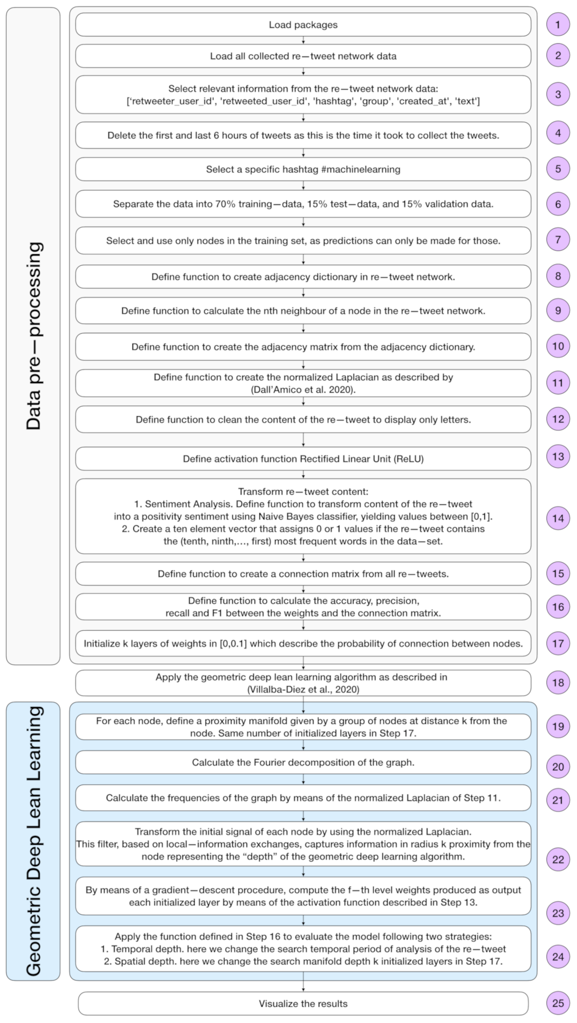
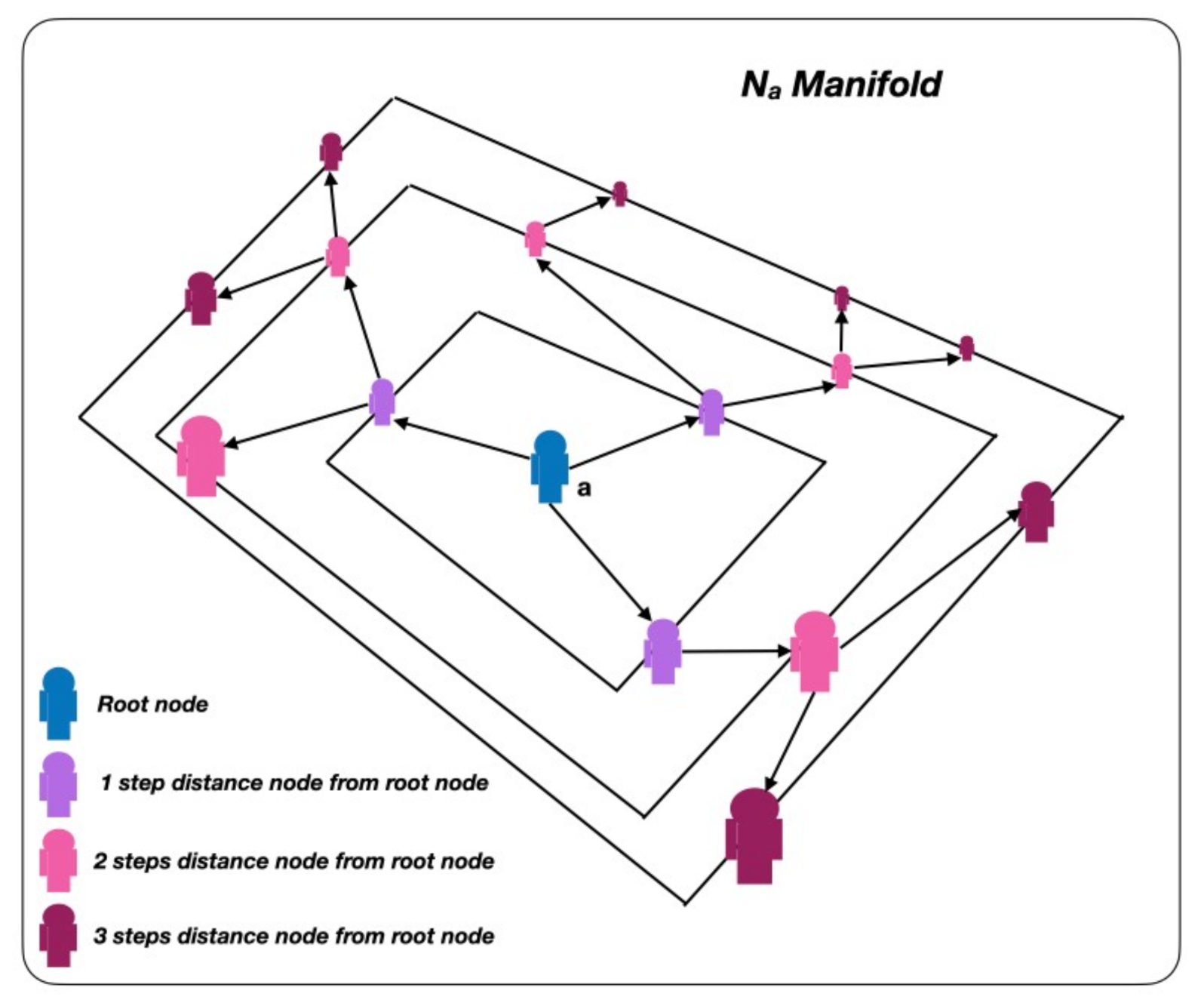
The algorithm is implemented following the mathematical formulation previously shown in [23]. A flow diagram of the algorithm is shown in Figure 1. As a rough outline, it would suffice to say that, as shown in Figure 2, for each a we define a proximity manifold given by a group of nodes at distance k from the node. This spatial manifold size is the third hyperparameter of the algorithm, which confers different learning properties and yields in different computational times.
We then initialise the weights or probabilities of the connection between the nodes in the interval . We perform a Fourier graph decomposition by eigendecomposing the reduced graph Laplacian matrix into eigenvalues and eigenvectors. Based on the Fourier decomposition of the reduced graph Laplacian, we calculate the graph frequencies which describe the graph structure. By means of the representation of the reduced graph Laplacian through the graph frequencies, the retweet signal between each node in the manifold is convoluted. This convolution operation lies at the heart of the geometric deep lean learning algorithm. The spatial depth of this convolutional operation is given by the number k of layers defined by the spatial depth of the manifold search.
3. Data Mining on Twitter
Social network analysis has seen a large rise since the advent of online social media networks and the resulting easier access to data [46]. The aim of the research can have different facets. It can include the analysis of information [47,48] and behaviour flow [49,50] or be used in the context of network theory [41]. In this field, Twitter, in particular, has rapidly become a source for research [51]. Twitter is a microblogging and social networking service that is one of the most popular global online social media sites, which is especially popular with a younger creative audience [52]. The interactions are through so-called tweets. These are messages that can be public posts or responses. Posts from other users that are resent are called retweets. Through this rebroadcasting of information, complex networks are formed. This network can be studied by methods developed in network theory.
Retweet networks on Twitter can be used and collected for different goals. These usually include semantic or network property analysis. In [53], a retweet network was built by mining the tweets of a specific group of users. Using the collected network, communities inside the European Parliament were able to be detected with high accuracy without knowing the ground truth. In a different approach, all tweets corresponding to a previously defined group of hashtags were collected to create a retweet network. By examining this data, organised trolling efforts were able to be detected [54]. The information contained in the nodes is structured and describes certain characteristics of the node such as its date of birth, gender, etc. controlled by the user. The edges of the network, the retweets, contain semi-structured information with a structured part that describes the temporal metadata of the retweet, as well as a non-structured part formed by its content.
In this Section 3, we will implement an example of data mining of the social network, as well as a detailed analysis of the obtained graph. As argued by Byrd and Turner [55], a single case study can be seen as a possible building block in the process of developing the validity and reliability of the proposed hypothesis. However, in this case, due to the standardised dataset structures involved in the social, we can accept the results as plausible and general. Following the recommendations of Eisenhardt [56], a clear case study road map is followed. This road map has several phases, namely, Section 3.1 experimental setup, Section 3.2 specification of population and sampling, Section 3.3 data collection, Section 3.4 standardisation procedure, and Section 3.5 data analysis. To ensure the replicability of the results obtained, the source code for data mining, tweet IDs, and network analysis is available under the Open Access Repository (https://github.com/danielschmidtschmidt/Geometric-deep-lean-learning-Evaluation-using-a-Twitter-social-network (accessed on 22 July 2021)) which was created with Jupyter Lab Version 1.2.6.
3.1. Experimental Setup
To mine the social network data from Twitter, an official application programming interface (API) is provided that can be used for different purposes, including academic research. In August 2020, Twitter announced version 2.0 with added features that, among other improvements, aid academic research by allowing further access. For this work, version 1.1 of the API is used. It is the newest stable version during the writing of this work and offers the needed features for the aggregation of the data. A paid and a free version of the API are available that mainly differ by the limits that are placed on the number of data that can be collected in a time frame. In addition, the time range to receive older tweets with the paid version is higher. This makes some tasks difficult or impossible, only using the free version.
For the chosen retweet network, tweets are selected by searching for specific hashtags. With the free version, only tweets of the last seven days can be garnered, although this step can be repeated to receive continuous data over a longer time frame. With this study, enough data could be collected in the 7-day time frame. Although some missing tweets can be expected for the free version [57], it is not anticipated to have a measurable influence on this research. To use the Twitter API, an application for a developer account must be filed. Therein, the use case needs to be stated. This can be used for academic research. Only the redistribution of the tweet IDs from the collected data is permitted. With these tweet IDs, the contained content of the tweets can be requested through the Twitter API. Therefore, only the tweet IDs of the collected tweets in this research can be shared.
The following software was used in this research for the collection, visualisation, and analysis of the retweet network:
- Programming language: Python 3.7.6 [58];
- Python wrapper for the Twitter API: Tweepy 3.8.0;
- Python package for the creation and study of complex networks: NetworkX 2.4 [59];
- Python plotting library: Matplotlib 3.1.3;
- Python package for data analysis and manipulation: Pandas 1.0.1;
- Network visualisation and exploration: Gephi 0.9.2 [60].
3.2. Specification of Population and Sampling
To examine the different forms of retweet networks, the three Twitter accounts of the journal were chosen as a starting point. For each, the 2000 most recent tweets of the Twitter accounts were inspected. The 25 most common hashtags of every account were selected and are visible in Table 1 with minimal overlap, as together these are 70 unique hashtags. This results in two different kinds of groups. A group formed by the tweets using a hashtag and by the group formed through a set of hashtags.
It is expected that this results in varied network properties, as different structures in these communities exist. Users using one of these hashtags do not necessarily form homogeneous groups, as they can appear in different contexts that do not have a big overlap. For example, #5g could be used by researchers to discuss technology. Moreover, it can be used to advertise it or discuss the cultural and societal implications of technology. Furthermore, all tweets form a network or, respectively, multiple networks that are not fully connected to each other.
3.3. Data Collection
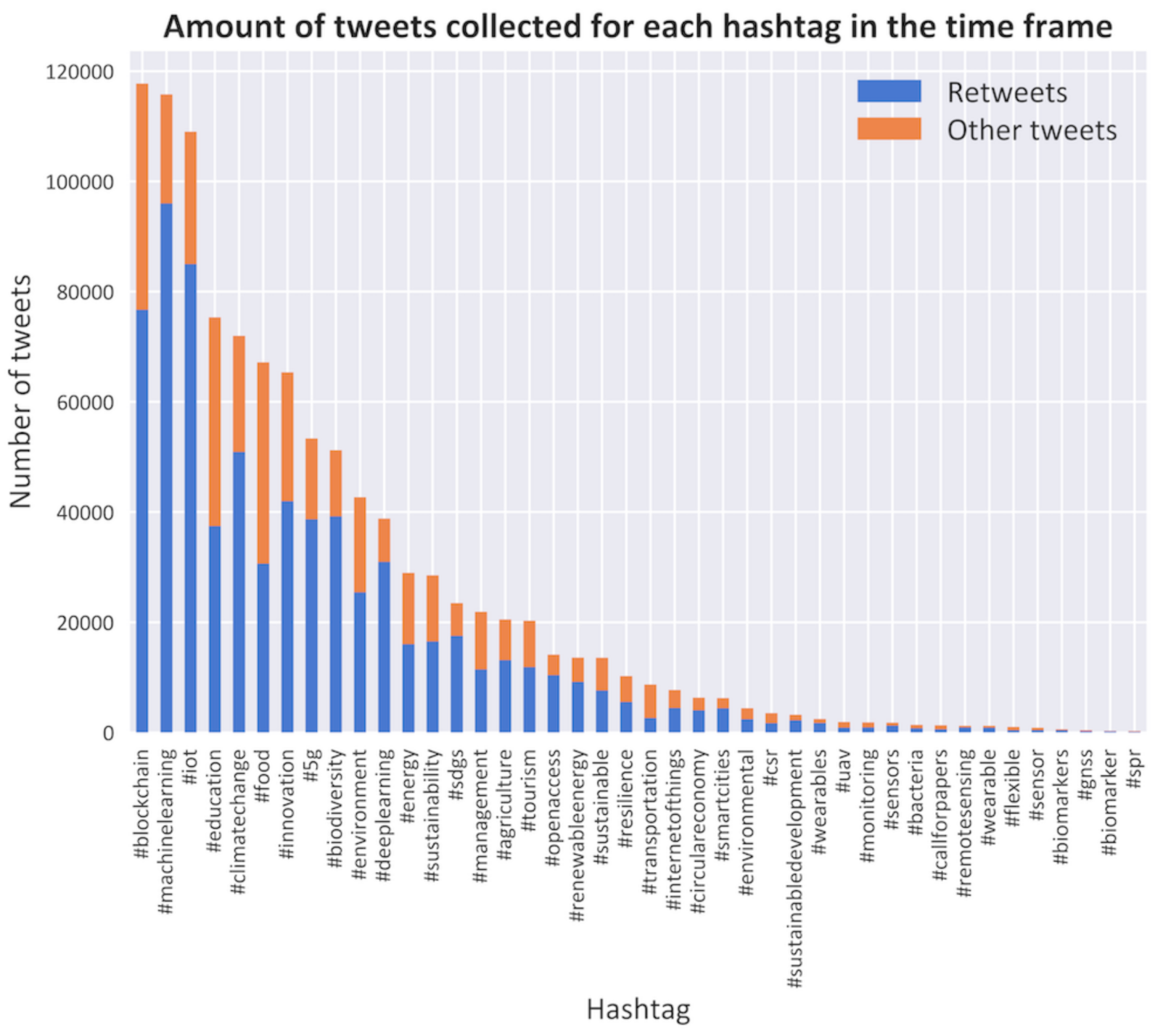
With API, all public tweets from 1 June 2020 at 13:50 until 9 June 2020 at 22:18 were collected that contained any of the 70 hashtags collected in Table 1. The number of tweets for each hashtag varies widely. This is visible in Figure 3, with only 42 of the 70 hashtags containing more than 100 retweets. It is possible to also take into account the tweets that are quotes and replies. The data include 71,741 quote tweets and 18,683 reply tweets. As this is only a small percentage of the total, only the retweets were used to build the network. Under both hashtags #machinelearning and #blockchain, 120,000 tweets were posted. For the hashtags #immunosensors and #i3s2017, there were no tweets available in the time frame. Especially biosensor-specific hashtags show a low number of tweets, with only 3800 tweets for all 25 hashtags. All collected tweets sum up to 1,060,319, and with almost two-thirds being retweets, 689,995 retweets were collected.
3.4. Standardisation Procedure
To have the same time frame for the tweets of all hashtags, the time passed during the collection of the tweets has to be taken into account. As this was almost 6 h, the first and last 6 h of tweets were deleted. This makes the data more comparable.
It would be possible to collect the same number of tweets for each hashtag. As this would mean a different time frame for the collection of each hashtag or removing some tweets, this is not useful for the analysis. All in all, this is also a property of the network.
3.5. Data Analysis
In the data analysis phase, two different approaches are taken. The first is to gain an understanding of the network by visualising the network, which has always been an important part of network research [61]. Qualitative insights can be developed and communicated in a direct way. The second is to analyse the social network’s properties.
Although it is possible to model a retweet network as a bipartite network [62], the retweet network was built as a non-directed network. In it, the users build the nodes and the edges are formed by a retweet. This allows an easier analysis. Our focus is set on a shared connection through the information retweeted. The created network focuses on the same interests and views of the users. All retweets in the specific time frames are used to create the non-directed retweet network. For the retweet, both the original writer and the user retweeting it are added to the nodes. Furthermore, a link is added between those two users. For the time frames, only one link between the two users is added and analysed. This action is repeated for all retweets. If the nodes are not already part of the network, these are added.
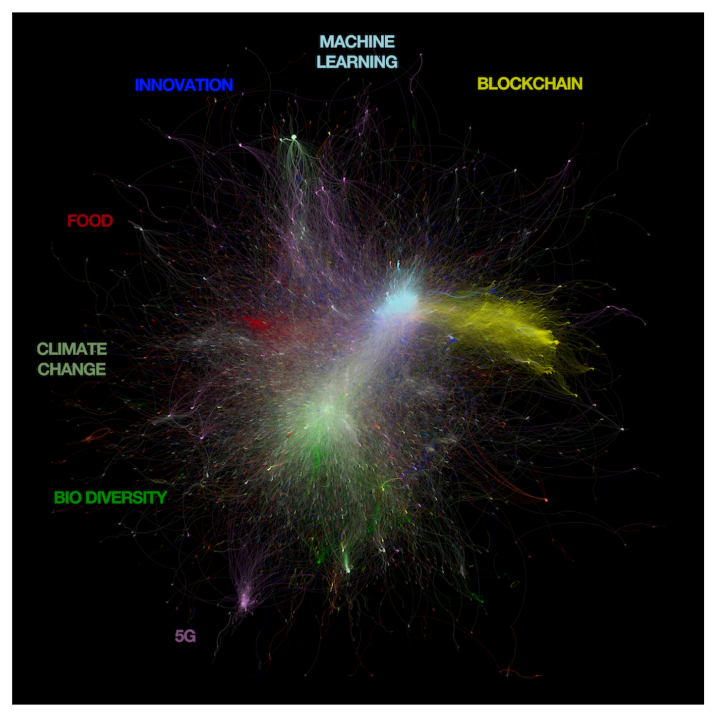
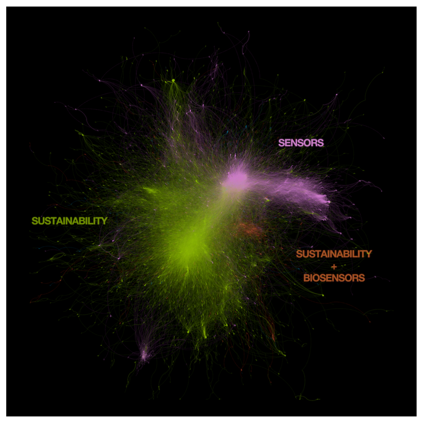
The visualisation of the retweet network in Figure 4 gives an overview and easier understanding of the complex network that is formed by the retweets. The figure shows in various colours the network of MDPI journals under study. It should be noted that not all retweets of the users are displayed, as only the tweets using the predefined hashtags form this network. Additionally, only the biggest connected component is shown as the unconnected parts of the network would be pushed to the edges of the image by the force-directed algorithm [63]. The hashtags of seven dominant groups are added in the image for easier identification, with the same colour and near to their biggest cluster.
The visualisation offers the following useful qualitative information:
- For most tweets of the dominant hashtags, distinct communities are formed that mostly have interactions with users that also use that hashtag. The strength of the interconnection can be seen by the density of the communities. Users with the #machinelearning tweets are at close distance, which indicates a high level of connectedness. This, in turn, is a sign that a low average path length and a high clustering coefficient exists within this group. On the other hand, #blockchain has a further stretched the patch, which indicates a higher average path length and lower clustering coefficient. These differences can be seen for all dominant tweets.
- Strong points of contact and overlap can be seen between some groups. As could be expected, one of the strongest can be seen between the tweets of #climatechange and #biodiversity, but also between #machinelearning and #blockchain, although the connection is weaker and limited to specific parts of the network, which is probably due to the users discussing the technical side of both. Strong connections can also be seen in other parts. This demonstrates the overlap of some communities.
- Although clear communities for #5g are visible, these are separated. This can be traced to the fact that it can be used in different contexts. More importantly, it can be used in tweets that are written in different languages, which is rarely the case with other hashtags, as they most often have a translation for that language.
The boundaries of the communities are even clearer through the classification by the journal. Most users are connected to other users in the respectable group. This can be seen in Figure 5 and is to be expected, as the hashtags of a journal form groups of similar interest. Only the two major groups and the smaller groups which are clearly visible form distinct communities. Most visible outliers can be traced back to #5g.
However, this analysis is particularly interesting due to being able to quantify the structure of the network, its nodes and edges, as well as the signals that characterise these elements. That is why we will now make a quantitative description of our findings.
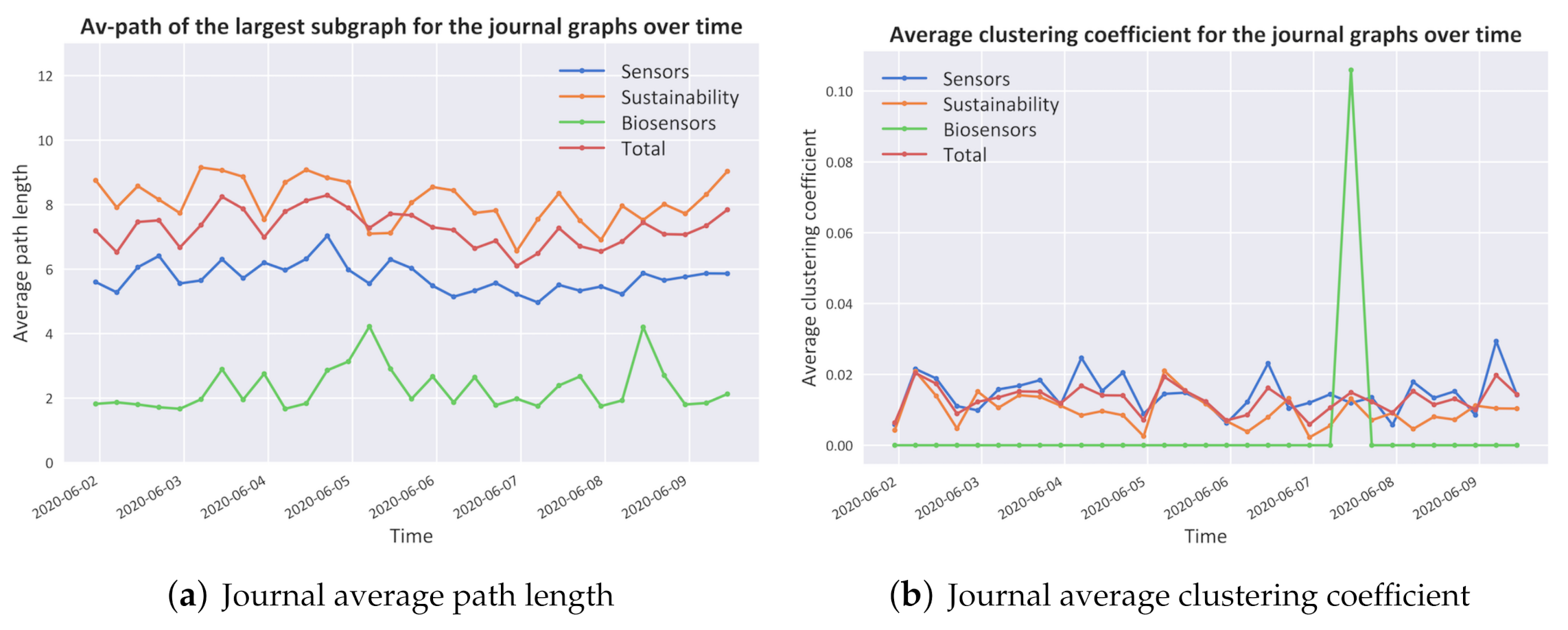
- Network StructureAs shown in Figure 6, the dataset presents a typical log–log long-tailed degree distribution which is typical of small-world/scale-free networks with a degree exponent of [41].In Figure 7, several other network metrics are shown. Specifically, in Figure 7a, the average path length, which is defined as the average number of steps along the shortest paths for all possible pairs of network nodes of all journals, is proved to be in the range which, together with the representation in Figure 7b of the high clustering coefficients, which is a measure of the degree to which nodes in a graph tend to cluster together, show a typical behaviour of small-world networks evolving towards a scale-free network topology [41].
- Network SignalsThe information contained in each retweet network about the nodes and edges can be mined in a semi-structured standard given by the platform. A truncated for our purposes example of a retweet is shown in Table 2.After this inspection, it will be easy for the reader to recognise that all information, both for the nodes and for the edges, except the text field, is structured. The information contained in the text field, which is the content of the retweet, can be considered as unstructured since it is given by the user who composes it.
4. Geometric Deep Lean Learning Evaluation
To validate the proposed geometric deep learning algorithm [23] and its use of the data—the set obtained in Section 3 —a study road map with several phases is tailored for the algorithm implementation as follows: Section 4.1 experimental setup, Section 4.2 data preprocessing explanation, Section 4.3 hyperparameter description, and Section 4.4 data analysis and results.
4.1. Experimental Setup
The experiments in this study were implemented with a computer equipped with an Intel(R) Xeon(R) Gold 6154 3.00GHz CPU and an NVIDIA Quadro P4000 Graphic Process Unit (GPU) with 96 GB of random access memory (RAM). The operating system was Red Hat Linux 16.04 64-bit version. When additional computational power was needed, Amazon Web Services and Azure ecosystem were employed [64].
The following software was used in this research for the collection, visualisation, and analysis of the retweet network:
- Programming language: Python 3.7.6 [58];
- Python plotting library: Matplotlib 3.1.3;
- Python package for data analysis and manipulation: Pandas 1.0.1;
- Python package for scientific computing and array calculation: Numpy 1.18.0.
4.2. Data Preprocessing
To facilitate a more efficient further processing, the relevant data concerning the structure and evolution of the retweet content are structured for further processing. The structure of the data is shown in Table 3.
Because it takes six hours to collect the data from the Twitter application programming interface (API), the first and last six hours of the retweets are deleted to ensure a clean and balanced dataset. To further focus the study framework, we inspect the network of retweets with the hashtag #machinelearning. To more effectively analyse the content of the retweet, we eliminate all contents that are not letters.
As described in Section 2, the content of the retweets is semi-structured and therefore must be transformed to ensure proper processing. For this purpose, we substitute the retweet content with a vector of 11 classes. The first element contains the result of the based standard sentiment analysis naive Bayes classifier algorithm [65], which allows a prior classification of the retweets by assigning them a score in the interval [0,1], into negative (values close to 0), neutral (values around 0.5) or positive (values close to 1). The rest of the 10 categories describe with binary classification, 0 or 1 if the retweet content contains 1, 2, 3, ..., or the 10 most used words in the overall retweet network, respectively.
4.3. Geometric Deep Lean Learning Hyperparameters
We implement the function defined to measure the performance of the model and compute its accuracy following two strategies: (1) variation of temporal depth t in which we change the search temporal period of analysis of the retweet following a standard time series split cross-validation method [66] and (2) spatial depth k in which we change the number of layers. Our model will predict the probability that a node will connect to another node, taking into account the structure and content of the time-dependent network.
The hyperparameter design decision depends on the dataset structure. Our geometric deep lean learning algorithm presents two hyperparameters: temporal depth and spatial depth search. In this specific case, we chose a temporal depth of days. Furthermore, we chose a spatial manifold depth search of because of the dataset size and related computational time.
4.4. Data Analysis and Results
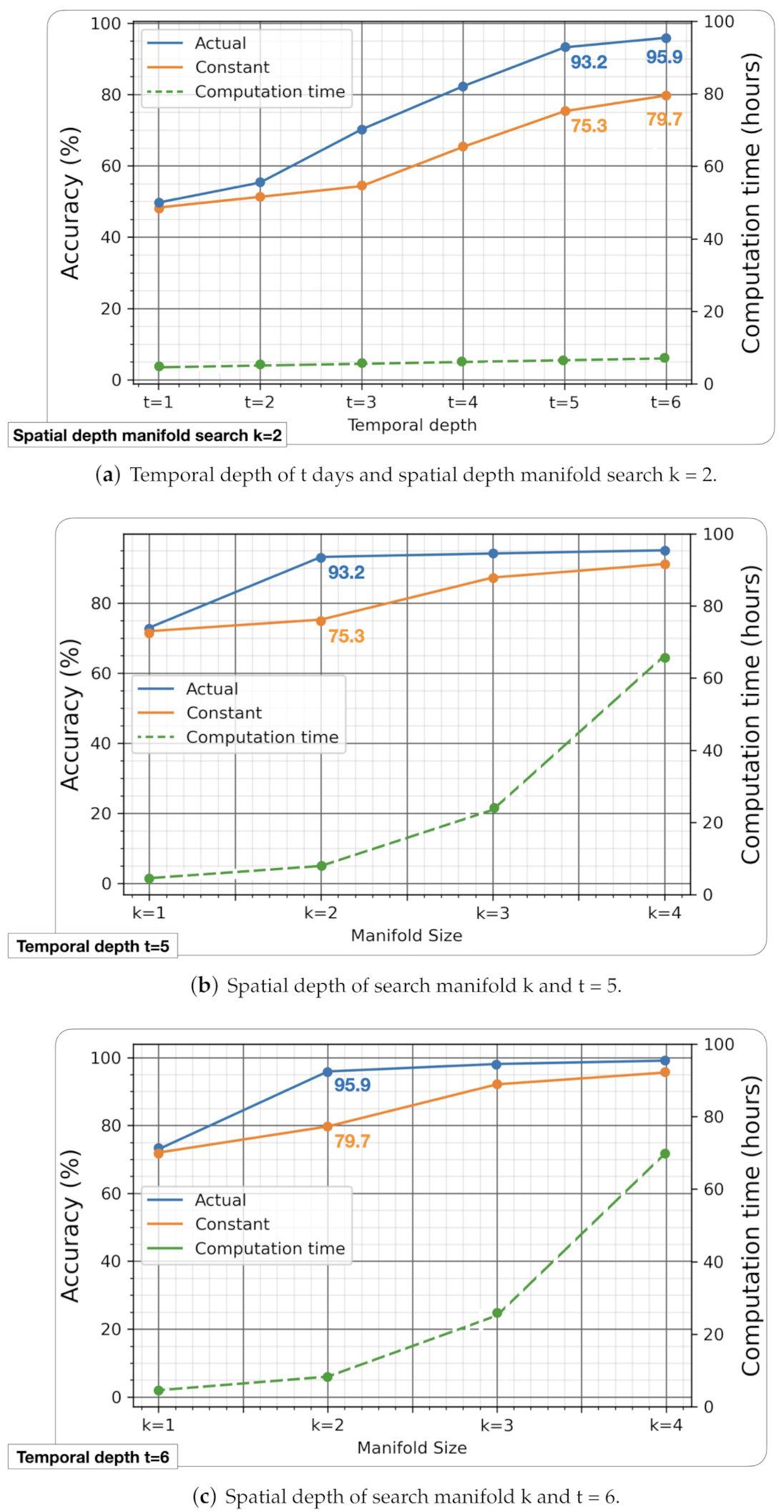
The geometric deep lean learning algorithm aims to predict the probability that two nodes will join in the future by learning from the evolution of the structure and content of the graph. As outlined in Section 4.2, we have applied this algorithm to two different signals with the same graph structure: one with the actual retweet content transformed through a naive Bayes and binary classification and one with the content of constant retweets (zero variability). To achieve the optimum computational time measured in hours, accuracy measured in %, and the cost of data mining, expressed by the temporal depth measured in days, we performed several experiments which are summarised in Figure 8.
- As shown in Figure 8a we perform several experiments for different temporal depth with a constant spatial depth of the search manifold of .
- As shown in Figure 8b,c, we performed several experiments for different spatial depths of the search manifold with a constant temporal depth of and , respectively.
5. Discussion
We inspected the retweet network of three journals by means of data mining techniques to obtain empirical evidence of the performance of the algorithm.
As we explained in Section 4, we performed two types of experiments: one in which we varied the temporal depth of our search while keeping the spatial depth of the search manifold constant, and vice versa.
To validate the performance of the model, we used [1].titfuture dataset. we combined contingency classes (TRUE, FALSE) and (connection, no-connection), hence building four categories: true negative (TN) is not a connection and has been predicted as a no-connection category; false positive (FP) is not a connection and has been predicted as a connection category; false negative (FN) is a connection but has been predicted as a no-connection category; true positive (TP) is a connection and has been predicted as a connection category. Derived from this categorisation, the performance measurement of accuracy can typically be measured by Acc = (TN + TP)/(TN + FP + FN + TP) [67]. Although another alternative way to measure the link prediction is to measure the area under the receiver operating characteristic curve (AUC) [68], we chose in this work to measure the accuracy because AUC ignores the predicted probability values and the goodness of fit of the model; it is only truly informative when there are true instances of absence available, and the objective is the estimation of the realised distribution. Moreover, AUC does not give information about the spatial distribution of model errors, which is a key feature in our geometric deep lean learning model [69].
We will now discuss the results of these experiments in detail.
5.1. Variation of Temporal Depth with Constant Spatial Depth
The results in Figure 8a show a linear growth of computation time t with the temporal depth of our search. The results show different behaviours depending on the content of the retweet. The geometric deep lean learning algorithm presents a typical sigmoid learning curve when the content of the retweets is actual or constant, and the accuracy of the model with actual content is always better than the one with constant content. This suggests that the algorithm is indeed extracting relevant information from the content of the retweet. This learning allows it to achieve better accuracy rates than in the case where the content of the retweet is constant, where the algorithm can only learn from the structure of the network since all nodes have the same information. The peak learning point is reached at a maximum time depth of days and with 95.2% of accuracy, followed by 93.2% attained for a slightly lower time depth of days and .
5.2. Variation of Spatial Depth with Constant Temporal Depth
The results in Figure 8b,c show an exponential growth of the computation time t with the spatial depth k of the search manifold of the form with and a coefficient of determination of in both cases. The exponential increase of computation time with the spatial depth of the search manifold enabled us to seek a practicable compromise solution. In industrial environments, computation time is a determining factor when integrating computational algorithms into real-time processes. The results show different behaviours depending on the content of the retweets. We can observe that the geometric deep lean learning algorithm learns better with real information from the retweets than with constant information. Specifically, on the one hand, in Figure 8b, we can observe how with a search manifold depth of only and , thus keeping a low computational time, the algorithm shows a performance of 93.2% with real information, versus 75.3% with constant information. On the other hand, in Figure 8c, we can observe how a search manifold depth of only and a linear increase in the temporal depth search , thus keeping the computational cost under control, the algorithm shows a performance of 95.9% with real information, versus 79.7% with constant information. Although in both cases, the performance of the algorithm increases to values above 99% with a search manifold depth of , this is at a high computational cost. For these reasons, we deem as the best optimum solution obtained with a temporal depth of , spatial depth of the manifold search .
The results of these combined experiments show the intrinsic value of our algorithm: on the one hand, they allow us to show what effects the signals contained in the nodes have on the predictive ability of the algorithm, and on the other, they show its predictive power.
6. Conclusions and Management Implications
In summary, our application shows how we can use a new deep learning model applied to non-Euclidean topologies such as complex graphs to predict the links that will occur in the network using the information contained in the network structure and within the nodes of the network. Specifically, we combined deep learning methods such as gradient descent and modified convolution on local manifolds at each node, with preprocessing techniques of complex sparse network structures and standard sentiment analysis naive Bayes and binary classifier algorithms. Our application of the geometric deep lean learning algorithm allows us to predict, with high probability and low computational cost, the evolution of a graph derived from a real complex network of retweets. We have also shown that the application of the algorithm is able to achieve this by means of a novel convolution process applied to non-Euclidean topology that takes into account both the time-dependent topology of the graph and the time-varying signals occurring within it.
The implications for the management of this novel application are profound since they allow predicting the evolution of networks associated with Industry 4.0 creation systems by taking into account their topology and the information contained within them. This provides insight into the potential evolution of the system. For example, we can predict which nodes are most likely to connect in a logistic chain or which process occurs—the owner node is most likely to connect within a chain of command. This could greatly help in the appropriate strategic organisational design, as the predictive geometric deep lean learning algorithm would anticipate possible less likely configurations. Our algorithm has therefore the potential to be integrated into an expert decision support system that helps industry leaders improve their decision-making process and could therefore help increase the performance of the associated value-creating processes.
Furthermore, for our Twitter dataset, the naive Bayes sentiment and binary classification allowed us to preprocess the dataset adequately and attain acceptable performance levels with low computational resources. When applying the geometric deep lean learning algorithm to Industry 4.0 cyber–physical networks, future challenges lie in finding a suitable representation of the semi-structured data that allows increasing the performance of the geometric deep learning algorithm on the real data with adequate levels of both the temporal depth and spatial depth of the search manifold and therefore with less computational time. The limitations of this work are limited to the analysis of complex time-dependent networks in which the temporal or spatial depth is too large to be computed. In an Industry 4.0 or Internet of Things environment, such topologies are to be expected. To overcome these obstacles, the authors envision the formation of suitable clusters, for example, based on expert knowledge, upon application of the geometric deep lean learning algorithm.
Author Contributions
Conceptualisation, J.V.-D. and M.M.; methodology, J.V.-D. and M.M.; software implementation, J.V.-D., D.S. and M.M.; validation, J.V.-D., M.M. and D.S.; formal analysis, J.V.-D., D.S. and M.M.; writing—original draft preparation, J.V.-D. and M.M.; writing—review and editing, J.V.-D. and M.M.; visualisation, D.S.; supervision, M.M. All authors have read and agreed to the published version of the manuscript.
Funding
J.V.-D. would like to acknowledge the Spanish Agencia Estatal de Investigacion, through research project code RTI2018-094614-B-I00 into the “Programa Estatal de I+D+i Orientada a los Retos de la Sociedad”.
Data Availability Statement
To ensure the replicability of the results obtained, the source code for data mining, tweet IDs, and network analysis is available under the Open Access Repository (https://github.com/danielschmidtschmidt/Geometric-deep-lean-learning-Evaluation-using-a-Twitter-social-network accessed on 22 July 2021) which was created with Jupyter Lab Version 1.2.6.
Conflicts of Interest
The authors declare no conflict of interest.
Abbreviations
The following abbreviations are used in this manuscript:
| API | Application programming interface |
| AUC | Area under the receiver operating characteristic curve |
| MDPI | Multidisciplinary Digital Publishing Institute |
References
- Reinsel, D.; Gantz, J.; Rydning, J. The Digitization of the World. From Edge to Core. 2018. Available online: https://resources.moredirect.com/white-papers/idc-report-the-digitization-of-the-world-from-edge-to-core (accessed on 2 April 2021).
- Froelicher, D.; Troncoso-Pastoriza, J.R.; Sousa, J.S.; Hubaux, J. Drynx: Decentralized, Secure, Verifiable System for Statistical Queries and Machine Learning on Distributed Datasets. IEEE Trans. Inf. Forensics Secur. 2020, 15, 3035–3050. [Google Scholar] [CrossRef]
- Verbraeken, J.; Wolting, M.; Katzy, J.; Kloppenburg, J.; Verbelen, T.; Rellermeyer, J.S. A Survey on Distributed Machine Learning. ACM Comput. Surv. 2020, 53. [Google Scholar] [CrossRef] [Green Version]
- Diène, B.; Rodrigues, J.J.; Diallo, O.; Ndoye, E.H.M.; Korotaev, V.V. Data management techniques for Internet of Things. Mech. Syst. Signal Process. 2020, 138, 106564. [Google Scholar] [CrossRef]
- Savaglio, C.; Ganzha, M.; Paprzycki, M.; Bădică, C.; Ivanović, M.; Fortino, G. Agent-based Internet of Things: State-of-the-art and research challenges. Future Gener. Comput. Syst. 2020, 102, 1038–1053. [Google Scholar] [CrossRef]
- Ordieres-Mere, J.; Villalba-Diez, J.; Zheng, X. Challenges and Opportunities for Publishing IIoT Data in Manufacturing as a Service Business. Procedia Manuf. 2019, 39, 185–193. [Google Scholar] [CrossRef]
- Khan, W.; Rehman, M.; Zangoti, H.; Afzal, M.; Armi, N.; Salah, K. Industrial internet of things: Recent advances, enabling technologies and open challenges. Comput. Electr. Eng. 2020, 81, 106522. [Google Scholar] [CrossRef]
- Evjemo, L.D.; Gjerstad, T.; Grøtli, E.I.; Sziebig, G. Trends in Smart Manufacturing: Role of Humans and Industrial Robots in Smart Factories. Curr. Robot. Rep. 2020, 1, 35–41. [Google Scholar] [CrossRef] [Green Version]
- Jardim-Goncalves, R.; Romero, D.; Grilo, A. Factories of the future: Challenges and leading innovations in intelligent manufacturing. Int. J. Comput. Integr. Manuf. 2017, 30, 4–14. [Google Scholar] [CrossRef]
- Huang, Q.; He, H.; Singh, A.; Lim, S.N.; Benson, A.R. Combining Label Propagation and Simple Models Out-performs Graph Neural Networks. arXiv 2020, arXiv:2010.13993. [Google Scholar]
- Frasca, F.; Rossi, E.; Eynard, D.; Chamberlain, B.; Bronstein, M.; Monti, F. SIGN: Scalable Inception Graph Neural Networks. arXiv 2020, arXiv:2004.11198. [Google Scholar]
- Löwe, S.; Madras, D.; Zemel, R.; Welling, M. Amortized Causal Discovery: Learning to Infer Causal Graphs from Time-Series Data. arXiv 2020, arXiv:2006.10833. [Google Scholar]
- Johnson, D.D.; Larochelle, H.; Tarlow, D. Learning Graph Structure With A Finite-State Automaton Layer. arXiv 2020, arXiv:2007.04929. [Google Scholar]
- Rossi, E.; Chamberlain, B.; Frasca, F.; Eynard, D.; Monti, F.; Bronstein, M. Temporal Graph Networks for Deep Learning on Dynamic Graphs. arXiv 2020, arXiv:2006.10637. [Google Scholar]
- Kumar, S.; Zhang, X.; Leskovec, J. Predicting Dynamic Embedding Trajectory in Temporal Interaction Networks. In Proceedings of the 25th ACM SIGKDD International Conference on Knowledge Discovery & Data Mining, Anchorage, AK, USA, 4–8 August 2019; Volume 2019, pp. 1269–1278. [Google Scholar] [CrossRef]
- Noorshams, N.; Verma, S.; Hofleitner, A. TIES: Temporal Interaction Embeddings for Enhancing Social Media Integrity at Facebook. arXiv 2020, arXiv:2002.07917. [Google Scholar]
- Wang, X.; Lyu, D.; Li, M.; Xia, Y.; Yang, Q.; Wang, X.; Wang, X.; Cui, P.; Yang, Y.; Sun, B.; et al. APAN: Asynchronous Propagation Attention Network for Real-time Temporal Graph Embedding. arXiv 2020, arXiv:2011.11545. [Google Scholar]
- Bronstein, M.M.; Bruna, J.; LeCun, Y.; Szlam, A.; Vandergheynst, P. Geometric deep learning: Going beyond euclidean data. IEEE Signal Process. Mag. 2017, 34, 18–42. [Google Scholar] [CrossRef] [Green Version]
- Monti, F.; Otness, K.; Bronstein, M.M. Motifnet: A Motif-Based Graph Convolutional Network for Directed Graphs. In Proceedings of the 2018 IEEE Data Science Workshop (DSW), Lausanne, Switzerland, 4–6 June 2018; pp. 225–228. [Google Scholar] [CrossRef] [Green Version]
- Zhang, Z.; Cui, P.; Zhu, W. Deep Learning on Graphs: A Survey. IEEE Trans. Knowl. Data Eng. 2020. [Google Scholar] [CrossRef] [Green Version]
- Mayer, R.; Jacobsen, H.A. Scalable Deep Learning on Distributed Infrastructures: Challenges, Techniques, and Tools. ACM Comput. Surv. 2020, 53, 1–37. [Google Scholar] [CrossRef] [Green Version]
- Lei, N.; An, D.; Guo, Y.; Su, K.; Liu, S.; Luo, Z.; Yau, S.T.; Gu, X. A Geometric Understanding of Deep Learning. Engineering 2020, 6, 361–374. [Google Scholar] [CrossRef]
- Villalba-Diez, J.; Molina, M.; Ordieres-Mere, J.; Sun, S.; Schmidt, D.; Wellbrock, W. Geometric Deep Lean Learning: Deep Learning in Industry 4.0 Cyber–Physical Complex Networks. Sensors 2020, 20, 763. [Google Scholar] [CrossRef] [PubMed] [Green Version]
- Duvenaud, D.; Maclaurin, D.; Aguilera-Iparraguirre, J.; Gómez-Bombarelli, R.; Hirzel, T.; Aspuru-Guzik, A.; Adams, R.P. Convolutional Networks on Graphs for Learning Molecular Fingerprints. arXiv 2015, arXiv:1509.09292. [Google Scholar]
- Stankovic, L.; Mandic, D.; Dakovic, M.; Brajovic, M.; Scalzo, B.; Li, S.; Constantinides, A.G. Graph Signal Processing—Part III: Machine Learning on Graphs, from Graph Topology to Applications. arXiv 2020, arXiv:2001.00426. [Google Scholar]
- Chen, L.C.; Barron, J.T.; Papandreou, G.; Murphy, K.; Yuille, A.L. Semantic Image Segmentation with Task-Specific Edge Detection Using CNNs and a Discriminatively Trained Domain Transform. arXiv 2015, arXiv:1511.03328. [Google Scholar]
- Velardi, P.; Navigli, R.; Cucchiarelli, A.; D’Antonio, F. A New Content-Based Model for Social Network Analysis. In Proceedings of the 2008 IEEE International Conference on Semantic Computing, Santa Clara, CA, USA, 4–7 August 2008; pp. 18–25. [Google Scholar] [CrossRef]
- Stilo, G.; Velardi, P. Time Makes Sense: Event Discovery in Twitter Using Temporal Similarity. In Proceedings of the 2014 IEEE/WIC/ACM International Joint Conferences on Web Intelligence (WI) and Intelligent Agent Technologies (IAT), Warsaw, Poland, 11–14 August 2014; Volume 2, pp. 186–193. [Google Scholar] [CrossRef]
- Chen, J.; Zhang, J.; Xu, X.; Fu, C.; Zhang, D.; Zhang, Q.; Xuan, Q. E-LSTM-D: A Deep Learning Framework for Dynamic Network Link Prediction. IEEE Trans. Syst. Man Cybern. Syst. 2021, 51, 3699–3712. [Google Scholar] [CrossRef] [Green Version]
- Yao, L.; Wang, L.; Pan, L.; Yao, K. Link Prediction Based on Common-Neighbors for Dynamic Social Network. Procedia Comput. Sci. 2016, 83, 82–89. [Google Scholar] [CrossRef] [Green Version]
- Evci, U.; Pedregosa, F.; Gomez, A.; Elsen, E. The Difficulty of Training Sparse Neural Networks. arXiv 2020, arXiv:1906.10732. [Google Scholar]
- Zhang, M.; Chen, Y. Link Prediction Based on Graph Neural Networks. arXiv 2018, arXiv:1802.09691. [Google Scholar]
- Shang, K.K.; Li, T.C.; Small, M.; Burton, D.; Wang, Y. Link prediction for tree-like networks. Chaos Interdiscip. J. Nonlinear Sci. 2019, 29, 061103. [Google Scholar] [CrossRef]
- Zhou, L.K.; Yang, Y.; Ren, X.; Wu, F.; Zhuang, Y. Dynamic Network Embedding by Modeling Triadic Closure Process. In Proceedings of the Thirty-Second AAAI Conference on Artificial Intelligence, (AAAI-18), the 30th Innovative Applications of Artificial Intelligence (IAAI-18), and the 8th AAAI Symposium on Educational Advances in Artificial Intelligence (EAAI-18), New Orleans, LA, USA, 2–7 February 2018; pp. 571–578. [Google Scholar]
- Keller, M. Curvature, Geometry and Spectral Properties of Planar Graphs. Discret. Comput. Geom. 2011, 46, 500–525. [Google Scholar] [CrossRef] [Green Version]
- Wu, Z.; Menichetti, G.; Rahmede, C.; Bianconi, G. Emergent complex network geometry. Sci. Rep. 2015, 5, 10073. [Google Scholar] [CrossRef] [Green Version]
- Bianconi, G.; Rahmede, C.; Wu, Z. Complex quantum network geometries: Evolution and phase transitions. Phys. Rev. E Stat. Nonlinear Soft Matter Phys. 2015, 92, 022815. [Google Scholar] [CrossRef] [Green Version]
- Bianconi, G.; Rahmede, C. Complex Quantum Network Manifolds in Dimension d > 2 are Scale-Free. Sci. Rep. 2015, 5, 13979. [Google Scholar] [CrossRef] [PubMed] [Green Version]
- Saleh, M.; Esa, Y.; Mohamed, A. Applications of Complex Network Analysis in Electric Power Systems. Energies 2018, 11, 1381. [Google Scholar] [CrossRef] [Green Version]
- Villalba-Diez, J.; Ordieres-Mere, J. Improving manufacturing operational performance by standardizing process management. Trans. Eng. Manag. 2015, 62, 351–360. [Google Scholar] [CrossRef]
- Barabási, A.L. Network Science; Cambridge University Press: Cambridge, UK, 2016. [Google Scholar]
- Villalba-Diez, J. The Lean Brain Theory. Complex Networked Lean Strategic Organizational Design; CRC Press: Boca Raton, FL, USA; Taylor and Francis Group LLC: Boca Raton, FL, USA, 2017. [Google Scholar]
- Dall’Amico, L.; Couillet, R.; Tremblay, N. A unified framework for spectral clustering in sparse graphs. arXiv 2020, arXiv:2003.09198. [Google Scholar]
- Harris, K.D.; Aravkin, A.; Rao, R.; Brunton, B.W. Time-varying Autoregression with Low Rank Tensors. arXiv 2019, arXiv:1905.08389. [Google Scholar]
- Wang, Y.; Yuan, Y.; Ma, Y.; Wang, G. Time-Dependent Graphs: Definitions, Applications, and Algorithms. Data Sci. Eng. 2019, 4, 352–366. [Google Scholar] [CrossRef] [Green Version]
- Borgatti, S.P.; Everett, M.G.; Johnson, J.C. Analyzing Social Networks; Sage: London, UK, 2018. [Google Scholar]
- Kim, J.; Hastak, M. Social network analysis: Characteristics of online social networks after a disaster. Int. J. Inf. Manag. 2018, 38, 86–96. [Google Scholar] [CrossRef]
- Arafeh, M.; Ceravolo, P.; Mourad, A.; Damiani, E.; Bellini, E. Ontology based recommender system using social network data. Future Gener. Comput. Syst. 2021, 115, 769–779. [Google Scholar] [CrossRef]
- Centola, D. The spread of behavior in an online social network experiment. Science 2010, 329, 1194–1197. [Google Scholar] [CrossRef] [PubMed]
- Arafeh, M.; Ceravolo, P.; Mourad, A.; Damiani, E. Sampling Online Social Networks with Tailored Mining Strategies. In Proceedings of the 2019 Sixth International Conference on Social Networks Analysis, Management and Security (SNAMS), Granada, Spain, 22–25 October 2019; pp. 217–222. [Google Scholar] [CrossRef]
- Ovadia, S. Exploring the potential of Twitter as a research tool. Behav. Soc. Sci. Libr. 2009, 28, 202–205. [Google Scholar] [CrossRef]
- Sloan, L.; Morgan, J.; Burnap, P.; Williams, M. Who tweets? Deriving the demographic characteristics of age, occupation and social class from Twitter user meta-data. PLoS ONE 2015, 10, e0115545. [Google Scholar] [CrossRef] [PubMed] [Green Version]
- Cherepnalkoski, D.; Mozetic, I. A retweet network analysis of the European Parliament. In Proceedings of the 2015 11TH International Conference on Signal-Image Technology & Internet-Based Systems (SITIS), Bangkok, Thailand, 23–27 November 2015; pp. 350–357. [Google Scholar]
- Stewart, L.G.; Arif, A.; Starbird, K. Examining trolls and polarization with a retweet network. In Proceedings of the ACM WSDM, Workshop on Misinformation and Misbehavior Mining on the Web, Los Angeles, CA, USA, 9 February 2018. [Google Scholar]
- Byrd, T.; Turner, D. Measuring the flexibility of information technology infrastructure: Exploratory analysis of a construct. J. Manag. Inf. Syst. 2000, 17, 167–208. [Google Scholar]
- Eisenhardt, K. Building theories from case study research. Acad. Manag. Rev. 1989, 14, 532–550. [Google Scholar] [CrossRef]
- Morstatter, F.; Pfeffer, J.; Liu, H.; Carley, K.M. Is the sample good enough? Comparing data from twitter’s streaming api with twitter’s firehose. arXiv 2013, arXiv:1306.5204. [Google Scholar]
- van Rossum, G. Python Tutorial, Technical Report CS-R9526; Centrum voor Wiskunde en Informatica (CWI): Amsterdam, The Netherlands, 1995. [Google Scholar]
- Hagberg, A.; Swart, P.; Chult, D.S. Exploring Network Structure, Dynamics, and Function Using NetworkX; Technical Report; Los Alamos National Lab. (LANL): Los Alamos, NM, USA, 2008.
- Bastian, M.; Heymann, S.; Jacomy, M. Gephi: An open source software for exploring and manipulating networks. In Proceedings of the Third International AAAI Conference on Weblogs and Social Media, San Jose, CA, USA, 17–20 May 2009; Volume 8, pp. 361–362. [Google Scholar]
- Freeman, L.C. Visualizing social networks. J. Soc. Struct. 2000, 1, 4. [Google Scholar]
- Bi, B.; Cho, J. Modeling a retweet network via an adaptive bayesian approach. In Proceedings of the 25th International Conference on World Wide Web, Montreal, QC, Canada, 11–15 April 2016; pp. 459–469. [Google Scholar]
- Jacomy, M.; Venturini, T.; Heymann, S.; Bastian, M. ForceAtlas2, a continuous graph layout algorithm for handy network visualization designed for the Gephi software. PLoS ONE 2014, 9, e98679. [Google Scholar] [CrossRef] [PubMed]
- Wali, M. Learn Microsoft Azure: Build, Manage, and Scale Cloud Applications Using the Azure Ecosystem; Packt Publishing: Birmingham, UK, 2018. [Google Scholar]
- Loria, S. Textblob Documentation. 2020. Available online: https://buildmedia.readthedocs.org/media/pdf/textblob/latest/textblob.pdf (accessed on 3 April 2021).
- Sheridan, R.P. Time-Split Cross-Validation as a Method for Estimating the Goodness of Prospective Prediction. J. Chem. Inf. Model. 2013, 53, 783–790. [Google Scholar] [CrossRef]
- Chollet, F. Deep Learning with Python; Manning Publications Co.: Shelter Island, NY, USA, 2018. [Google Scholar]
- Lü, L.; Zhou, T. Link prediction in complex networks: A survey. Phys. A Stat. Mech. Appl. 2011, 390, 1150–1170. [Google Scholar] [CrossRef] [Green Version]
- Jiménez-Valverde, A. Insights into the area under the receiver operating characteristic curve (AUC) as a discrimination measure in species distribution modelling. Glob. Ecol. Biogeogr. 2012, 21, 498–507. [Google Scholar] [CrossRef]
Figure 1.
Geometric deep lean learning algorithm flow diagram.

Figure 2.
Manifold of a given node a of spatial depth .

Figure 3.
Amount of retweets and other tweets collected for the selected hashtags that contain more than 100 retweets.
Figure 3.
Amount of retweets and other tweets collected for the selected hashtags that contain more than 100 retweets.

Figure 4.
Retweet network: the edges between two users are coloured according to the associated hashtag of the retweet.
Figure 4.
Retweet network: the edges between two users are coloured according to the associated hashtag of the retweet.

Figure 5.
Retweet network as shown in Figure 4. The edges between two users are coloured according to the group of hashtags.
Figure 5.
Retweet network as shown in Figure 4. The edges between two users are coloured according to the group of hashtags.

Figure 6.
log–log long-tailed degree distribution of the retweet network.

Figure 7.
Properties of the journal graphs for every 6-hour time frame in a week of tweets.

Figure 8.
Summary of results.


Table 1.
The 25 most common hashtags of three journals for 2000 examined tweets.
| Sensors | Sustainability | Biosensors | |
|---|---|---|---|
| 1. | #mdpisensors | #mdpisustainability | #mdpibiosensors |
| 2. | #sensors | #sustainability | #biosensors |
| 3. | #iot | #sustainable | #sers |
| 4. | #deeplearning | #sushighlycitedpaper | #electrochemical |
| 5. | #biosensors | #climatechange | #fret |
| 6. | #machinelearning | #susinterestingpaper | #spr |
| 7. | #internetofthings | #energy | #biomarkers |
| 8. | #sensor | #sdgs | #i3s2017 |
| 9. | #wearable | #circulareconomy | #biomarker |
| 10. | #remotesensing | #sustainabledevelopment | #raman |
| 11. | #uav | #tourism | #biosensor |
| 12. | #structuralhealthmonitoring | #callforpapers | #immunoassay |
| 13. | #wearablesensors | #agriculture | #microfluidic |
| 14. | #wirelesssensornetworks | #transportation | #i3s2019 |
| 15. | #i3s2019 | #biodiversity | #microfluidics |
| 16. | #sensornetworks | #environment | #wearables |
| 17. | #sensing | #csr | #microarray |
| 18. | #5g | #management | #bacteria |
| 19. | #monitoring | #food | #aptamer |
| 20. | #smartcities | #renewableenergy | #sensors |
| 21. | #gnss | #openaccess | #flexible |
| 22. | #biosensor | #innovation | #bret |
| 23. | #blockchain | #education | #lab_on_chip |
| 24. | #sensorfusion | #resilience | #immunosensors |
| 25. | #highlyaccessedpaper | #environmental | #openaccess |
Table 2.
Semi-structured network retweet signal.
| ’created at:’ | Tue Jun 09 14:42:30 +0000 2020, |
| ’id’: | ’1270365661215240192’, |
| ’username’: | ’MedGIFT group’, |
| ’user id’: | ’1012268385789513729’, |
| ’text’: | ’We are hiring! |
| ’quoted user’: | ’id’: ’1270359799201443840’, ... |
| ...’user id’: ’2163570636’,... | |
| ...’username’: ’adepeursinge’ |
Table 3.
Structured network retweet signal.
| Sender | retweeted_user_id |
| Receiver | retweeter_user_id |
| Evolution | created_at |
| Content | hashtag, group and retweet text |
Publisher’s Note: MDPI stays neutral with regard to jurisdictional claims in published maps and institutional affiliations. |
© 2021 by the authors. Licensee MDPI, Basel, Switzerland. This article is an open access article distributed under the terms and conditions of the Creative Commons Attribution (CC BY) license (https://creativecommons.org/licenses/by/4.0/).
Share and Cite
MDPI and ACS Style
Villalba-Diez, J.; Molina, M.; Schmidt, D. Geometric Deep Lean Learning: Evaluation Using a Twitter Social Network. Appl. Sci. 2021, 11, 6777. https://doi.org/10.3390/app11156777
AMA Style
Villalba-Diez J, Molina M, Schmidt D. Geometric Deep Lean Learning: Evaluation Using a Twitter Social Network. Applied Sciences. 2021; 11(15):6777. https://doi.org/10.3390/app11156777
Chicago/Turabian StyleVillalba-Diez, Javier, Martin Molina, and Daniel Schmidt. 2021. "Geometric Deep Lean Learning: Evaluation Using a Twitter Social Network" Applied Sciences 11, no. 15: 6777. https://doi.org/10.3390/app11156777
Note that from the first issue of 2016, this journal uses article numbers instead of page numbers. See further details here.