Quantifying the Impact of Production Globalization through Application of the Life Cycle Inventory Methodology and Its Influence on Decision Making in Industry

Prado-Galiñanes, Humberto. J.; Domingo, Rosario

doi:10.3390/pr9081271

Open AccessFeature PaperArticle

Quantifying the Impact of Production Globalization through Application of the Life Cycle Inventory Methodology and Its Influence on Decision Making in Industry

by

Humberto. J. Prado-Galiñanes

^*,†

and

Rosario Domingo

^*

Department of Construction and Manufacturing Engineering, Universidad Nacional de Educación a Distancia (UNED), C/Juan del Rosal 12, 28040 Madrid, Spain

^*

Authors to whom correspondence should be addressed.

^†

Programa de Doctorado en Tecnologías Industriales.

Processes 2021, 9(8), 1271; https://doi.org/10.3390/pr9081271

Submission received: 2 June 2021 / Revised: 18 July 2021 / Accepted: 19 July 2021 / Published: 23 July 2021

(This article belongs to the Special Issue Optimization Technology of Greenhouse Gas Emission Reduction)

Download

Browse Figures

Versions Notes

Abstract

:

Industries are nowadays not only expected to produce goods and provide services, but also to do this sustainably. What qualifies a company as sustainable implies that its activities must be defined according to the social and ecological responsibilities that are meant to protect the society and the environment in which they operate. From now on, it will be necessary to consider and measure the impact of industrial activities on the environment, and to do so, one key parameter is the carbon footprint. This paper demonstrates the utility of the LCI as a tool for immediate application in industries. Its application shall facilitate decision making in industries while choosing amongst different scenarios to industrialize a certain product with the lowest environmental impact possible. To achieve this, the carbon footprint of a given product was calculated by applying the LCI method to several scenarios that differed from each other only in the supply-chain model. As a result of this LCI calculation, the impact of the globalization of a good’s production was quantified not only financially, but also environmentally. Finally, it was concluded that the LCI/LCA methodology can be considered as a fundamental factor in the new decision-making strategy that sustainable companies must implement while deciding on the business and industrial plan for their new products and services.

Keywords:

life cycle inventory; life cycle assessment; carbon footprint; environment; ecological responsibility; social responsibility; impact

1. Introduction

In rapidly changing industries, making the right decisions at the right time may establish the difference between a successful and a disastrous enterprise. In this regard, one of the crucial decisions of the moment concerns the role of every industry in environmental preservation [1]. With climate change threating our current society [2] and the generations to come, and the pressure that industries are facing in order to decrease their impacts on the environment [3], diverse opportunities and directions must be deeply analyzed to properly decide not only which business plan will provide the biggest turnover, but also what environmental cost will need to be afforded. The challenge for industries starts with the estimation of the environmental impact of their daily activities [4]. With the habit of just basing their strategy on pure financial figures, adopting another vision and understanding, evaluating, and measuring the cost also in terms of environmental degradation might not be as simple as expected. Thus, suitable tools must be provided to industries by the scientific community in order to facilitate the appropriate collection of facts and data, as well as to accelerate the analysis of different production alternatives to understand not only the financial, but also the environmental risk of a certain decision [5].

This paper shows on the one hand the potential of the life cycle inventory (LCI) [6,7] methodology once applied to the industrialization of a product, and on the other hand it represents, through the analysis of a simple practical case, the different outcomes that the carbon footprint (CF) [8] of a product may have, depending on the chosen industrial supply-chain concept and the reliability of the selected LCI database [6]. Moreover, despite the complexity that collecting, analysing, contrasting, and optimizing an LCI demands, it is evinced that its application to industrial cases provides a very detailed output, analysing every material and energy flow, considering the contribution of automation [9], globalization [10], management of the process waste, and product end of life [11], amongst others.

1.1. Motivation to Research and Create This Paper

The current revolution that society needs to face demands the full involvement of the scientific community, as well as the leaders of the industries that are impacting the environment the most. Thus, looking for new applications for the LCA [12] to properly assess the impact of the supply chain and providing real facts and data to prove the different impacts that a good industrialization strategy implies towards the nature, was the main motivation that triggered the creation of this paper. In addition, the need to be useful as an engineer and to produce not at any cost, but sustainably, triggered the necessary drive to investigate in this regard.

1.2. Main Hypothesis, Assumptions and Considerations of the Article

For an analysis of this magnitude, it is fundamental to define, as accurately as possible, the different features (Table 1) of the case or cases to be considered in the LCI and subsequent life cycle assessment (LCA) [13].

In the absence of reliable and precise data linked to a certain product or a service study that already has been performed, different hypotheses, assumptions, and considerations must be selected and clearly stated so that they show the reliability of the outcome of this paper’s LCI.

It is important to emphasize that the cases that are analyzed in this paper (Table 2) are just fictitious examples of production or industrial scenarios that may be part of metal-forming industrial activities, such as those carried out by automotive official equipment manufacturers (OEMs) and automotive component suppliers [14].

For each and every case described in Table 2, there was a considerable amount of data to be collected, analyzed, and deployed in the paper so that it could be used for the necessary calculations aimed at estimating the CF. In particular, this data will be split into the fields and subfields represented in Table 1 in such a way that it will thoroughly describe the industrial scenarios to be evaluated.

Once the necessary data is at the concerned industry´s disposal, the LCI process [13,15] shall move on to the next stage, which in this paper consists of the pertinent calculations that lead to estimating the CF [16] of the scenarios at stake (Table 2).

Within each field represented in Table 1, there will be information easily accessible and data that will be assumed due to lack of reliable sources and in order to have a first estimation of the CF for each scenario within a reasonable time so that it meets the general project milestones considered. In any case, each assumption will be clearly identified, as well as the expected uncertainty for the values stated in the document so that the scientific community is also aware of the potential risks or deviations once the full data is available.

1.3. Article Structure

The structure of the paper will be the following. First, the methodology, as well as the assumptions and main data needed to obtain the expected results and conclusions, will be meticulously explained. Afterward, there will be a detailed explanation of how these different sorts of data combined and treated in various equations (Appendix A) provide complete CF results.

Once these results are properly explained, it will also be emphasized which future applications [17] the results may have in the industry, as well as in other papers of a similar kind. The first section of the paper is the introduction to the main research subject. This section is composed of five main subsections, namely the motivation that lead to creating this paper; the explanation of the main hypothesis, assumptions, and considerations of the article; an explanation of the article’s structure, a remark concerning the importance of the veracity of the databases used; and finally a brief explanation of the anticipated results.

The next section consists of a brief but necessary literature review in which other references related to the main topic of this article, the LCA methodology applied to assessing the impact of the globalization of a product; are analyzed to provide a good foundation to the sections and subsections to come in the article.

Following the literature review, there is the section named “Materials and Methods”. As subsections, there is first the “Goal and Scope Definition” regarding the LCA flow diagram. Second of all, there is the “Inventory Analysis”, in which the all the variables and information necessary to calculate the carbon footprint (CF) of the analyzed product will be presented. Finally, there is a subsection named “Functional Unit”, which is indispensable for every LCA applied.

To continue, once the LCI is complete, the next section consists of presenting the total results. These results will be split into four subsections according to the LCA flow diagram stages mentioned in the “Materials and Methods” section. The first subsection will cover the results linked to the product boundary conditions, the second will represent the CF of “Stages 0 and 1: Raw Material and Final Good Production” and the third and fourth sections will include the results linked to “Stage 2: Product Lifetime Usage” and “Stage 3: Waste Management”.

Close to the end of the article, the results will be interpreted and discussed to comprehend their environmental impact in a section named “Results Interpretation and Discussion”, which in turn is divided into three subsections: the analysis of the fields with the highest GHG emissions, the consideration of the complexity of the LCI methodology, and finally the potential further application of the LCI method.

To finalize the research, the conclusions are deployed, followed by Appendix A, in which the main equations used to estimate the CF of the LCI are presented.

1.4. Veracity of the Database amd Countermeasures: Uncertainty Assessment

In a paper of this kind, the need to treat many different sorts of data from a great variety of sources (Table 1) may lead to an accumulation of smaller or larger calculation errors, which at the end of the day will impact the results and thereby the conclusions of this research document.

Thus, in order to provide reliable results, it is also important to consider the veracity of each source of information, as well as the assumptions. In this particular case, it will be communicated which sort of reliability level is considered for each kind of data and factors. For instance, a certain GHG assigned to a certain source (materials, energy, waste, etc.) may be accompanied by a reliability factor of “X”% [18], which means that the results might vary within a certain range (X–100%), and this must be considered by the scientific community in order to make the right decisions while also pushing to have the lowest uncertainty for this objective. These uncertainties, for most of the LCAs, and in particular for the one deployed in this paper, are linked to the fact of making assumptions to fill “gaps” in the LCI creation, which are a crucial step to provide final and complete results [19].

1.5. Anticipated Results

It must be mentioned that for the products analyzed, we calculated a difference of +30.1% comparing the most polluting scenario (“3B”, considering there are different sub-scenarios that are also analyzed: A, B, and C) with the least globalized and thereby “greenest” scenario (“1”). We took this “Scenario 1” as reference for the ratio Equation (1):

R a t i o = \frac{C a r b o n f o o t p r i n t C a s e 3 B}{C a r b o n f o o t p r i n t C a s e 1},

(1)

The methodology and procedure to obtain the above result will be explained in the following article sections.

2. Literature Review

The LCA methodology is a standardized procedure (ISO 14,040 [12] and ISO 14,044 [12]) [20] that offers a tool to properly assess the impact of an entire product life cycle on a certain factor generally linked to the environment [21]. It has been already applied to different products and branches [15,22,23]; however, there is still some lack of knowledge within the industry for what the LCA utility concerns [24].

Its success as a methodology to provide a full environmental assessment of every variable embedded in a product’s life is based on the consideration of everything linked to the product itself [22], starting from the extraction of the raw material that composes it down to the processes for handling the product at its end of life (EOL) [22].

The Sustainable Development Goals urge the decarbonization of industrial activities [25,26], particularly for sectors as crucial as energy production and transportation [27]. Thus, it is indispensable to analyze the impact of every stage of the life cycle of the products manufactured and services provided by those sectors. Thereby, the scientific community shall be able to advise the industry so that it makes the right decisions in the right fields and with the appropriate efforts so that decarbonization comes at the expected pace.

Every manufactured good, especially those for which production and sales are globalized and that are pressed by highly demanding customers, especially for what the manufacturing cost of every good concerns [28], is playing a crucial role in climate change and the global CF. The reason is that the supply chain reaches further locations seeking lower material and production costs [29], often forgetting the environmental impact of such a strategy [30].

The need to rapidly industrialize new goods to come in a certain industry prevents the proper assessment of the entire business plan that the company commits to follow. Thus, a tool like the LCA needs to be more easily usable for the industry [31], providing a quick and reliable outcome for items such as supply panel impact, logistics footprint [32,33], and transport mean utilization impact [34], amongst others.

Although globalization cannot be easily prevented, and while from an economic growth and even social perspective it would not be desirable, it has to be applied in accordance with sustainability principles. Thus, its overall environmental footprint (environmental footprint families [35]) needs to be always considered so that the least-polluting and harmful option is the one always selected by those in charge of industrializing the product or service production.

3. Materials and Methods

The main method that is used in this analysis consists of the application of the LCA [36] standards to define the CF [37] of the different production scenarios (Table 2) for the same product life stages.

The basis of every LCA consists of creating the best LCI possible [38], with this being the main target of the investigation and results deployed in this scientific article.

3.1. Goal and Scope Definition

The main goal of this LCA consists of analyzing the production of a certain product (Figure 2) considering a series of scenarios whose main difference consists of the supply-chain definition (Table 2). The scenarios vary from a centralized production with considerably short distances between suppliers, the main production factory, and the customer nodes; to a very wide production footprint where the material and components suppliers are based in Asia, for instance, and the distribution or dispatch center and the sales market are located in Europe.

The outcome of the LCI will be the determination of the CF for each of the scenarios. This CF will be measured in kg of CO_2e. Once the CF is properly calculated for all the different product life cycle stages represented in the Figure 1, the production will be evaluated from an environmental point of view as well, differentiating the amount of production cases considered and concluding which one of those would provoke the lowest damage to the environment. It is also important to emphasize that the LCA scope will cover the entire product life customized for each scenario following the different stages described in Figure 1.

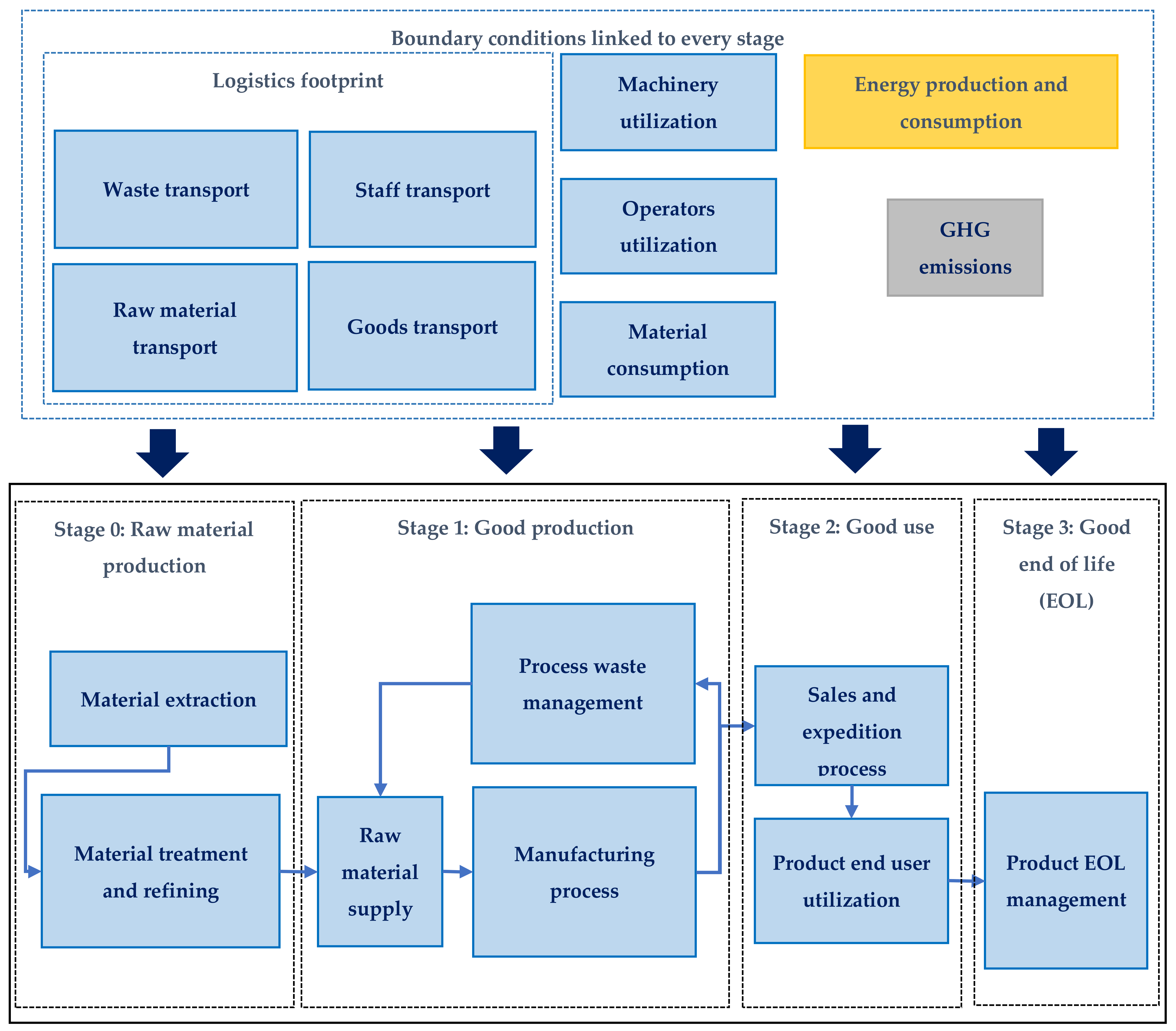
LCA Process Flow Diagram

The LCI will be carried out following the diagram represented in Figure 1. For more details linked to the specifics of every stage or boundary condition, Table 1 provides all necessary information.

The same diagram will be followed and applied to every scenario analyzed (Table 2). The difference between all three scenarios will be made by the variation on the boundary conditions.

3.2. Inventory Analysis

The necessary data that will constitute the LCI applied and that will be customized to every scenario will be divided into the following fields (Table 3), which represent a synthetized version of Table 1.

3.2.1. Equations Applied for Each Analyzed Field in Order to Calculate Their CF

To be able to gather enough data to feed the CF calculator, it is necessary to understand how the calculations will need to be done and which input variables will be crucial for the LCI.

In this regard, all needed and utilized equations to calculate the CF of the concerned product can be found in Appendix A.

3.2.2. LCI Input Applied to the Scenarios Considered in the Paper

Once the mathematical approach is clearly defined, it is necessary to begin collecting the necessary data that will be input in the equations (Appendix A) in order to get the CF results in return.

In the following sections, the concrete data employed for the three different scenarios that are compared in this paper will be explained. This has a double target. On the one hand, the main CF driving factors for a certain industrial activity [39] are clearly illustrated; and on the other hand, the research explains the structure and data size that every LCI requires [40].

Product Features Considered in the LCI: Real Data as Well as Assumptions

The concerned LCI analysis starts by defining the product whose production and overall industrial impact is analyzed.

In this particular case, the product will consist of a pipe used typically as main component of the hydraulic or exhaust systems of a certain internal combustion engine vehicle (ICVE) (Figure 2).

The product body will be made of stainless steel material with a very high CF [41] and overall impact on nature and climate preservation [42]. Furthermore, there is also a polymeric material (Figure 2A,B) involved in the packaging (PET) and transport protection (PP) of the good (Table 4).

Goods and Staff Transport

The transport of goods and passengers represents one of the most polluting human activities [45] to nature. Thus, its role in the CF estimation must be fully understood to properly quantify the impact on the environment of the raw material, product components, and final good logistics, as well as the contribution of the staff commuting to the concerned production and distribution centers.

As a starting point, it is imperative to define where every industrial activity will occur (Table 5).

Once the location of the industrial activities is identified, it is necessary to define the supply-chain network. To achieve this, the different paths established between the network nodes involved also must be analyzed in order to define the distance to travel and the sort of transport mean suitable to cover this distance within the expected time (Table 6).

Once the supply chain is confirmed, it is necessary to specify the main transport means’ features (Table 7, Table 8, Table 9 and Table 10) that will dictate the contribution of the logistic activities to the overall product CF.

To be precise, the main information that is indispensable for obtaining reliable CF results using the appropriate equations (Appendix A) are the following: transport mean type, needed fuel or energy type, mean load capacity, total amount of material to be transported, CO_2e implied in the energy consumption, top and average speed for each vehicle, maximum and nominal power, vehicle fuel consumption, distance to be driven, and number of necessary trips to carry the goods and employees either to the delivery destination or concerned work center.

Road transport:

Table 7. Road transport used for short and intermediate distance trips for goods and staff transportation [46,47,48].

Transport Mean Type	Load Capacity (t)	CO_2e (kg/km)
Small and medium-sized LVE	0.5 *	0.135
Large LVE	0.5 *	0.213
Van (small commercial vehicle (CVE))	1 *	0.252
Light/intermediate-duty truck (IDT)	2 *	0.45
Long-range bus (LRB)	21 *	0.688
Heavy-duty truck (HDT)	43 *	0.678

* Assumption.

Air transport:

Table 8. Air transport used for long-distance goods shipment and passenger transportation [49,50].

Aircraft Model	CO_2e	Unit	Load Capacity (t)	Energy Used	Considered Ground Distance (km)
B777-200	17.8	kg/km	82.9	Kerosene	*
B777-200	3.16	kg/kg fuel	82.9	Kerosene	*
A330-cargo	24.15	kg/km	33.18	Kerosene	6339
B747-400	17.80	kg/km	82.9	Kerosene	*
A380	66.89	kg/km	63.98	Kerosene	888 km
A380	24.15	kg/km	25.88	Kerosene	6339 km
B737-600	20.27	kg/km	13.95	Kerosene	499 km
B747-400	40.64	kg/km	39.08	Kerosene	7500 km
B747-400	36.19	kg/km	31.2	Kerosene	8000 km

* No reliable information found.

Maritime transport:

Table 9. Marine transport used for long-distance shipments of goods [51,52,53,54].

Mean Features	Data	Comments
Type of ship	Cargo vessel	-
Main engine	MAN B & W 7S80MC-C (Mark 7)	Low-speed engine
Load capacity (t)	3000–5000	-
Average power (kW)	18,620	-
Fuel specific consumption (g/kWh)	160.9	Fully loaded vessel *
CO_2e generated (g/kWh)	647	Fully loaded vessel *
Average speed (navigation knots)	15	-
Average speed (km/h)	27.78	-
Energy/fuel used	Diesel	Marine diesel used *

* Assumption.

Rail transport:

Table 10. Rail transport used for intermediate- and short-distance travels for goods and passenger transportation [55].

Main Features	Train Models/Types
Main Features	IC	SPR	FT
Energy used	Electric	Electric	Electric
Catenary efficiency (%)	80%	80%	80%
Engine reference	VIRM VI	SLT VI	BR186
Wagons	6	6	28
Empty train weight (kg)	391,000	198,000	2,400,000
Sort of load	Passengers	Passengers	Goods
Maximum load (kg)	15,582	8400	1,614,000
Maximum power (kW)	2157	1755	5600
Maximum traction force (kN)	142.5	150	-
Top speed (km/h)	160	160	95

Energy Production and Consumption

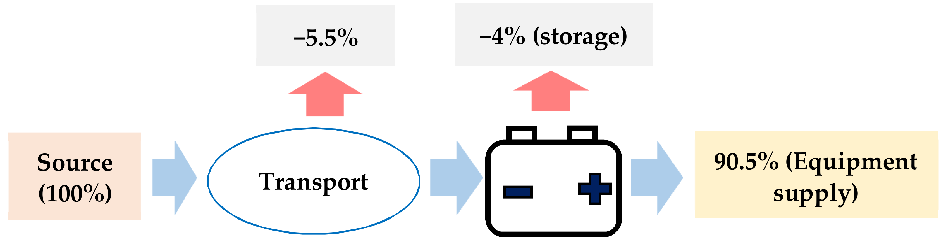
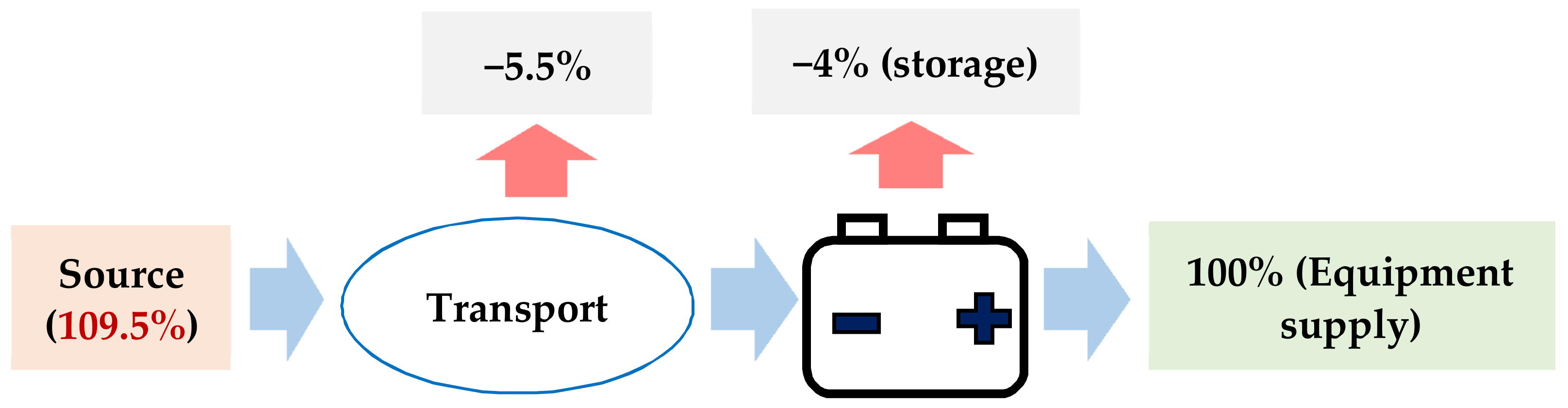
The energy sector is responsible for the most global GHG generation [45]. Thus, it is imperative to first properly consider the different sorts of energy that are utilized during all industrial activities (production and manipulation/logistics), and second, the CO_2e embedded in each fuel type.

In the analyzed industrial scenarios, the main sorts of energy were the following: electricity (Table 11), used in the product production and the rail transport of goods and passengers; gasoline and diesel (Table 12), used in the road and marine transport; and finally, kerosene, which is used in air transport (Table 8).

Energy Transport and Storage Efficiency

This section considers the fact of having inefficiencies during energy transport and storage, this being especially important for the transport and storage of electricity (Table 13), as this is a crucial factor that contributes to increases in GHG emissions during energy utilization.

The CF increase is due to the fact that, in order to compensate for the inefficiency during the electricity transport, as well as during the time the electricity remains stored in a certain battery, the electricity production at the source needs to be increased by at least the same percentage as the inefficiency that needs to be covered.

Increasing the energy consumption will thereby increase the GHG generation (CO_2e). In this case, it is expected to be an increase of 9.5% (Figure 3 and Figure 4).

Raw Material, Intermediate, and Final Product Production

It is important to emphasize that to be able to provide a reliable production CF, the following items need to be defined with the highest accuracy possible: production volume (Table 14), production time needed based on the process steps and process flow defined (Table 15, Table 16 and Table 17), product manufacturing cycle time (Table 18), equipment involved (Table 18, Table 19, Table 20, Table 21 and Table 22), equipment energy consumption (Table 18, Table 19, Table 20, Table 21 and Table 22), number of operators (Table 23), the production line automation level (Table 24) and the equipment efficiency (Table 25).

Product production features

Table 14. Main product industrial scenario—production features for the business case [62,63,64].

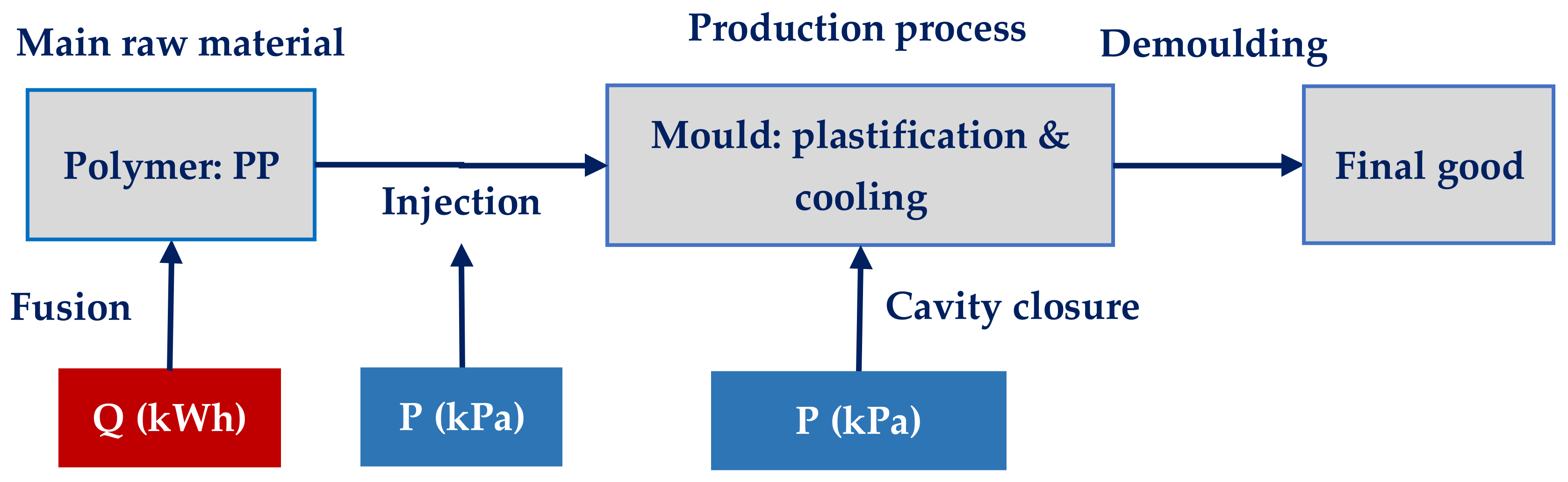
Features	Values	Unit
Production volume/sales (items)	200,000 *	(parts/year)
Production lifetime/duration (years)	5 *	(years)
Product manufacturing cycle time	65 *	(s)
Production time	3611	(h/year)
Working days (India)	250	(days)
Working days (Germany)	220	(days)
Working days (China)	249	(days)
Shifts a day (India)	2–3 *	-
Shifts a day (Germany)	2–3 *	-
Shifts a day (China)	2–3 *	-

* Assumed value to define the complete production scenario.

Raw material production

Raw material production has demonstrated to have one of the largest environmental impacts worldwide [65]. Many of the most common materials used, such as polymers (Figure 5) or metals (Figure 6), need massive amounts of energy and minerals to be manufactured and processed [66].

It is also important to emphasize the tough financial targets that many companies have in terms of material cost decrement and that provoke, under a pure economic assessment, that “greener materials” shall hardly ever defeat conventional ones (e.g., “green vs. conventional steel” [67]).

Table 15. Polymer injection energy and material consumption data [57].

Process.	Machine	Specific Energetic Consumption (SEC) (kWh/kg)	Type of Energy Used	Cycle Time (s)
Polymer injection	BOY 22E	0.9085	Hydraulic/electric	105

Figure 6. Steel production process [68]. Necessary to produce the main product structure/body (Table 4 and Table 17).

Table 16. Steel production energy and material consumption data [69].

Consumption		Unity	Details
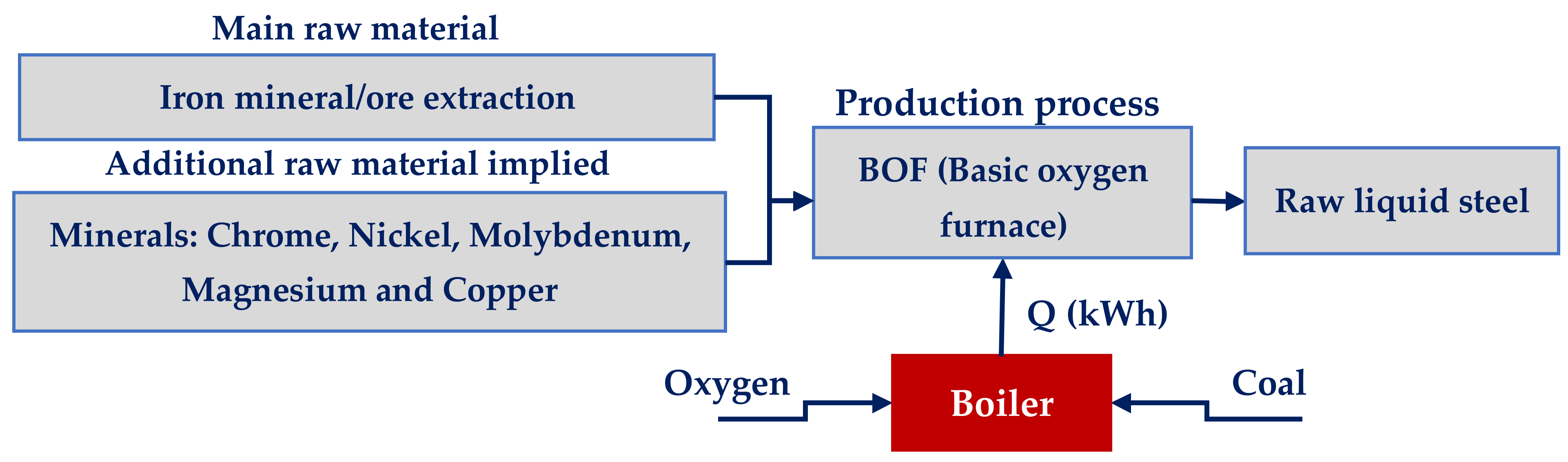
Energy	5555.56	(kWh/t)	Fossil fuel combustion
Agua	3300	(dm³/t)	-
CF	1.9	(t CO_2e/t Steel)	-

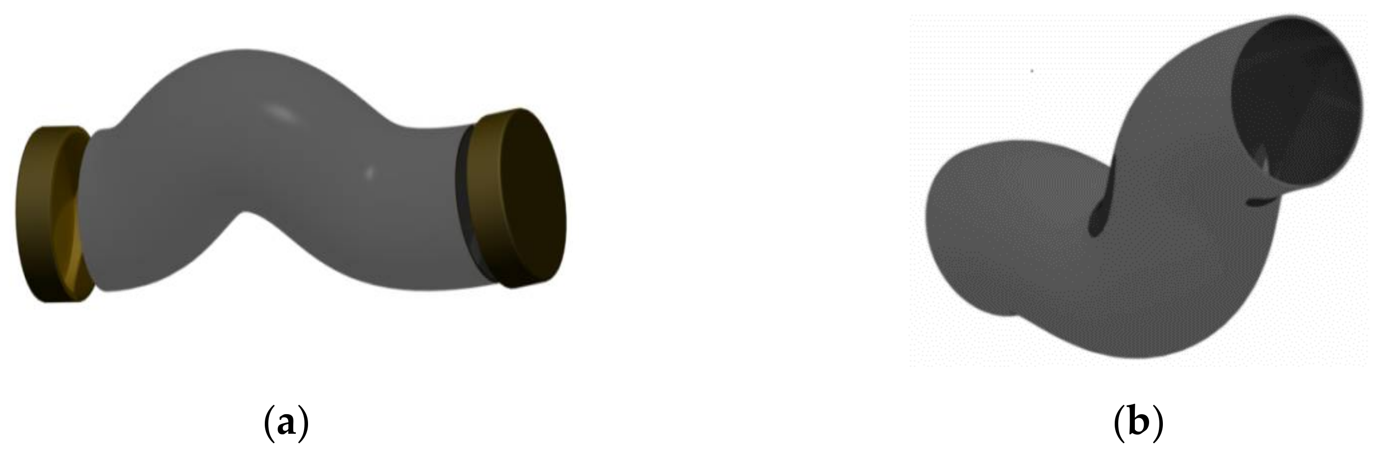
Main product manufacturing processes

Within the industrial operations of the concerned company, the production of the product is one of the main contributors toward climate change, and particularly toward its CF, currently the third-largest global contributor [45].

To be able to estimate the CF of the product-manufacturing process, the following items must be considered: different operations, from the raw material supply to the product packaging (Table 17); types and number of machines used, as well as their energy consumption (Table 18, Table 19, Table 20, Table 21 and Table 22); and finally the number of operators (Table 23) and robots or handling systems utilized at any stage of the product lifetime (Table 24).

Table 17. Manufacturing process description for the concerned product (Figure 2).

	Process Step	Description
1	Raw component supply	Steel tubes
2	Laser cutting	Adjusting the raw tube length to the product needs
3	Tube bending	Tube adopts the right shape
4	Tube stamping	Bent tube acquires necessary features
5	Tube CNC machining	Bent tube acquires necessary features and quality
6	Polymer protections assembly	Tube protections are assembled to protect the most important surfaces during shipment
7	Product quality control and packaging	Final quality check and packing prior to dispatching

Table 18. Laser-cutting equipment’s main features necessary for the CF calculation [70].

Feature	Value
Power (kW) (CO₂ as source)	4
Electric energy consumed
Cutting operation (kWh)	55.22
Secondary movements (kWh)	4.79

Table 19. Hydraulic bending cell’s main features necessary for the CF calculation [71].

Feature	Value
Number of movements	8
Hydraulic flow per machine movement (l/min)	41
Average hydraulic pressure (bar)	120
Power per movement (kW)	8.3

Table 20. Electric press’s main features necessary for the CF calculation [72].

Feature	Value
Servo consumption (kWs)	2742.7

Table 21. Five-axis CNC center’s main features necessary for the CF calculation [73].

Feature	Value
Electric power (kW)	44
Speed range (RPM)	0–10,000
Maximum torque (Nm)	242

Table 22. Robots’ main features necessary for the CF calculation [74].

	Model	Payload (kg)	Voltage (VAC)	Power (kW)
1	Yaskawa GP165R	165	380–480	4
2	Yaskawa GP50	50	380–480	3.6
3	Yaskawa AR2010	12	380–480	1.6

Table 23. Number of estimated/assumed operators involved in production.

Scenario	Steel Production	Polymer Production	Main Product Production	Main Product Assembly	Quality Check and Supervision	Product Dispatch
Scenario 1	0	0	0	0	4	1
Scenario 2	3	3	0	0	4	1
Scenario 3	3	3	2	1	4	1

Table 24. Number of estimated/assumed robots involved in the manipulation of different elements.

Scenario	Steel Production	Polymer Production	Main Product Production	Main Product Assembly	Product Dispatch
Scenario 1	2	2	2	2	1
Scenario 2	0	0	2	2	1
Scenario 3	0	0	1	0	1

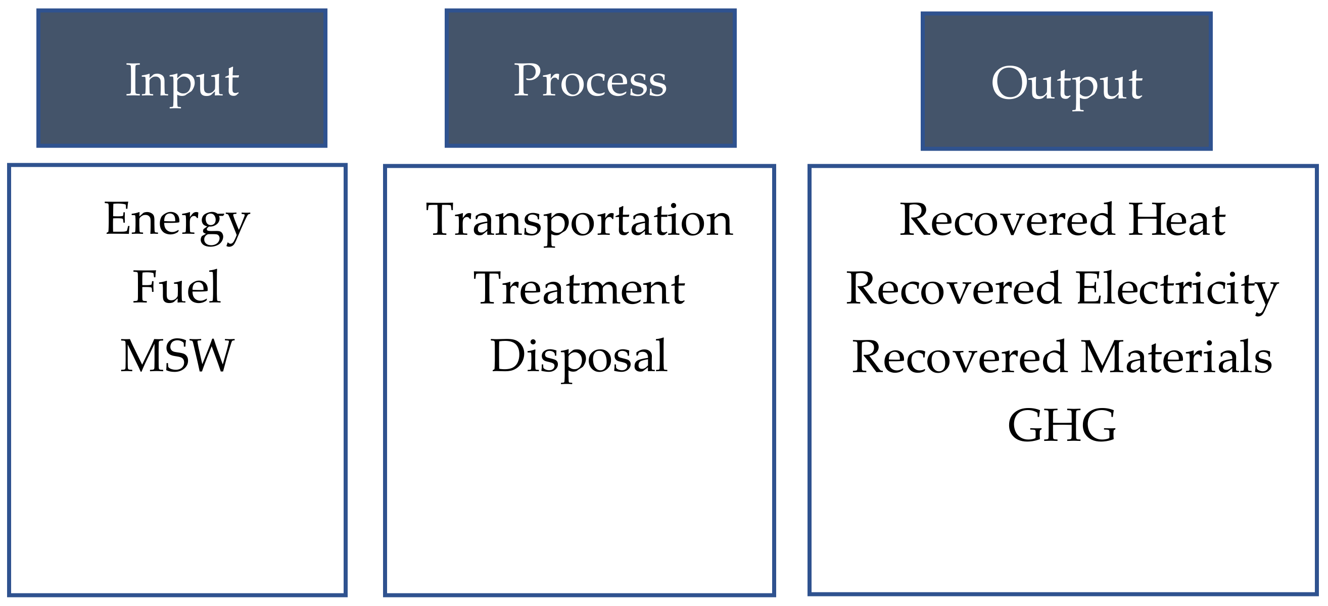
Product End-of-Life Management (Overall Waste Treatment)

Waste disposal and treatment represents one of the biggest issues for human society [75]. In this regard, waste disposal goes hand-in-hand with the CF of every product’s production and utilization. The reason is fairly simple: even if the CF of every industrial production activity linked to the analyzed product had a neutral or even negative result, there would be still a need to manage the end of life of the product itself. This is a complex task that, depending on the waste-disposal procedure and technology used, increases the CF considerably [76].

To properly estimate the overall CF of the total waste generated during the product’s life, it is necessary to understand and to classify the different sorts of waste that are created during every stage of the product’s manufacturing and following utilization.

Process waste

As for most of the analyzed fields (Section 3.2), the efficiency of every utilized process and machine possesses a crucial role in the CF estimate. Thus, comprehending the impact of this inefficiency on the treatment of the material is key to defining the amount of waste generated during the manufacturing process.

Table 25. Process efficiency of the main material-consuming and energy-demanding processes involved in the analyzed product’s production [77,78,79].

	Process	Implied Material	Process Efficiency	Comments
1	Pellet forming	PP and PE	95% *	Assumption
2	Plastic injection	PP and PE	99.59%	Due to preheating the granulated plastic, machine adjustments, and mould defects
3	Mineral extraction	Iron, chrome, nickel, etc.	76%	Considering the influence of the acid degradation using vanadium
4	Steel production	Iron	41.7%	For each tonne of raw steel, it is necessary to invest 2.4 tonnes of iron, amongst other additives
5	Casting	Steel EN 1.4507	95% *	Assumption
6	Forming and cutting	Steel EN 1.4507	90% *	Assumption: it is considered as 10% of technical scrap as a consequence of the different processes and machines used

* Assumption taken to move forward.

This amount of inefficiency represented in Table 25 unleashes an additional overproduction of the necessary materials (Table 26) to be able to guarantee that the final product will be composed of the expected amount of material regardless of the inefficiencies registered during the manufacturing processes.

Scaling the above values (Table 26) up to the final produced volumes (Table 14), it is possible to estimate the total amount of process waste Equation (2) that must be treated during the product’s production duration (Table 27).

T o t a l p r o c e s s w a s t e (k g) = P r o c e s s i n e f f i c i e n c y (%) \times T r e a t e d m a t e r i a l d u r i n g t h e p r o c e s s (k g / p r o d u c t) \times P r o d u c t l i f e t i m e p r o d u c t i o n (N u m b e r o f i t e m s)

(2)

Product End-of-Life (EOL) waste

First of all, the final amount of product waste, once it has been dismissed by the end user, must be quantified. To achieve that, it is necessary to know the final product sales (Table 14), as well as the final product weight (Table 4).

Using the above information as input in Equation (3) and breaking it down into the different materials used, the total generated waste can be deployed as illustrated in Table 28.

T o t a l p r o d u c t E O L w a s t e (k g) = T o t a l p r o d u c t s a l e s \times P r o d u c t w e i g h t (k g)

(3)

Waste-management location

Due to the fact that the waste-management strategy varies amongst different countries, it is crucial to understand on one hand where the process waste is caused (Table 4), and on the other hand, how the product sales are split within the targeted market (Table 29).

It is important to underline that in order to split the product EOL waste amongst a certain number of countries, it was assumed that the final market was only composed of several European countries, so the sales and thereby the waste generated by them were split according to the population of each concerned European country.

Waste-disposal methodologies considered for this LCI

Once the waste values have been estimated, it is important to consider two facts: the total waste split into the different management possibilities (landfilling, incineration [75], recycling [82], reusing, and Waste-to-Energy (WtE) [83], amongst others (Table 30 and Table 31)), and the different methodologies or technologies that are used to treat the split waste (Table 32, Table 33 and Table 34).

Considering that there are only three materials whose disposal needs to be managed, the waste split was evaluated only for the plastics (Table 30) and the steel (Table 31). Due to the difficulties encountered during the search of steel waste-management statistics, we considered the same split as for the municipal solid waste (MSW) (Table 31) in order to still be able to calculate the full CF of the total waste management.

Final Product Utilization (Item Use vs. Production)

To be able to estimate the GHG contribution of the product utilization, it was considered, as explained in the Section 3, that the produced good (Figure 2) would be assembled and used in different sorts of vehicles (Table 35).

The CF calculation was carried out by computing the information deployed in Table 35 and Equation (A25) (Appendix A).

Understanding the details represented in Table 35, the CF of each vehicle was calculated by gathering the GHG measured in grams per driven kilometers [48] and assuming a certain life expectancy for each sort of vehicle, which was measured in kilometers. The reason why the life expectancy of a passenger vehicle is considered to be shorter than the one of a commercial vehicle (Table 3) is because the utilization of a truck or a bus is considered to last longer than that expected of a lighter-utility vehicle.

Another important factor that will dictate the CF results is the weight of the analyzed item (Table 4), as well as the weight of the system in which it is assembled (Table 35). Due to the wide variety of vehicles available in the market, their weight needs to be carefully selected for both light vehicles (LVE) [46] and commercial vehicles (CVE) [48,87].

3.3. Functional Unit

As the standard ISO 14,040 mandates [12], for every LCA, it is crucial to define a functional unit that will allow the comparison of the different scenarios analyzed. In this particular case, the functional unit consists of the product composition (Table 4), manufacturing process steps (Table 17), and the sales amount and market (Table 14). Thus, in every scenario the same product volumes are produced following the same process steps, regardless of the variables that are selected. All the other parameters, such as energy use, amount of operators, level of automation, logistics footprint, or waste-management strategy, are dependent on the scenario to be treated. Due to this, they are defined as the input variables that, when applied to the functional unit, provide a different but comparable outcome for every scenario (CF).

4. Results

The results were obtained once the information contained in Section 3.2.2 was properly input in the equations illustrated in Appendix A. After compiling the equations output and splitting it into the different fields described throughout the paper (goods and staff transport, energy consumption linked to the product manufacturing process, energy transport and storage efficiency, product lifetime usage, and product and process waste management), the results of the LCI applied to the CF calculation can be presented.

The task that comes directly after collecting and treating the information in the appropriate equations consists of analyzing the output data in two steps:

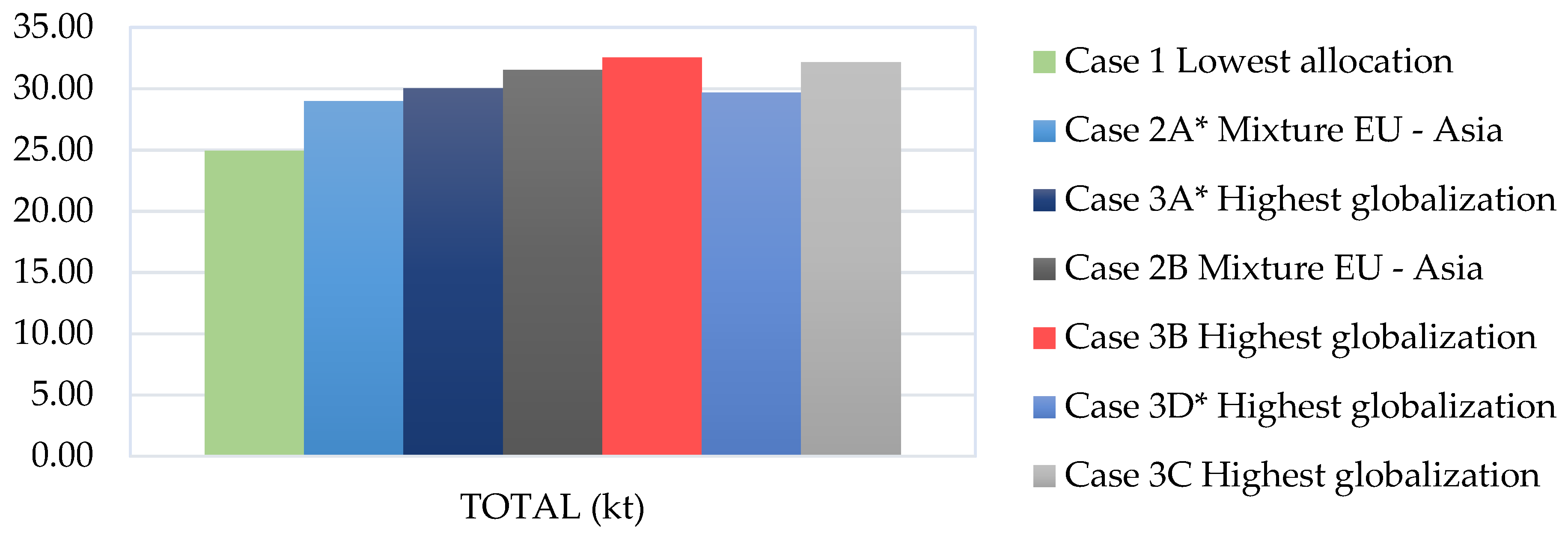
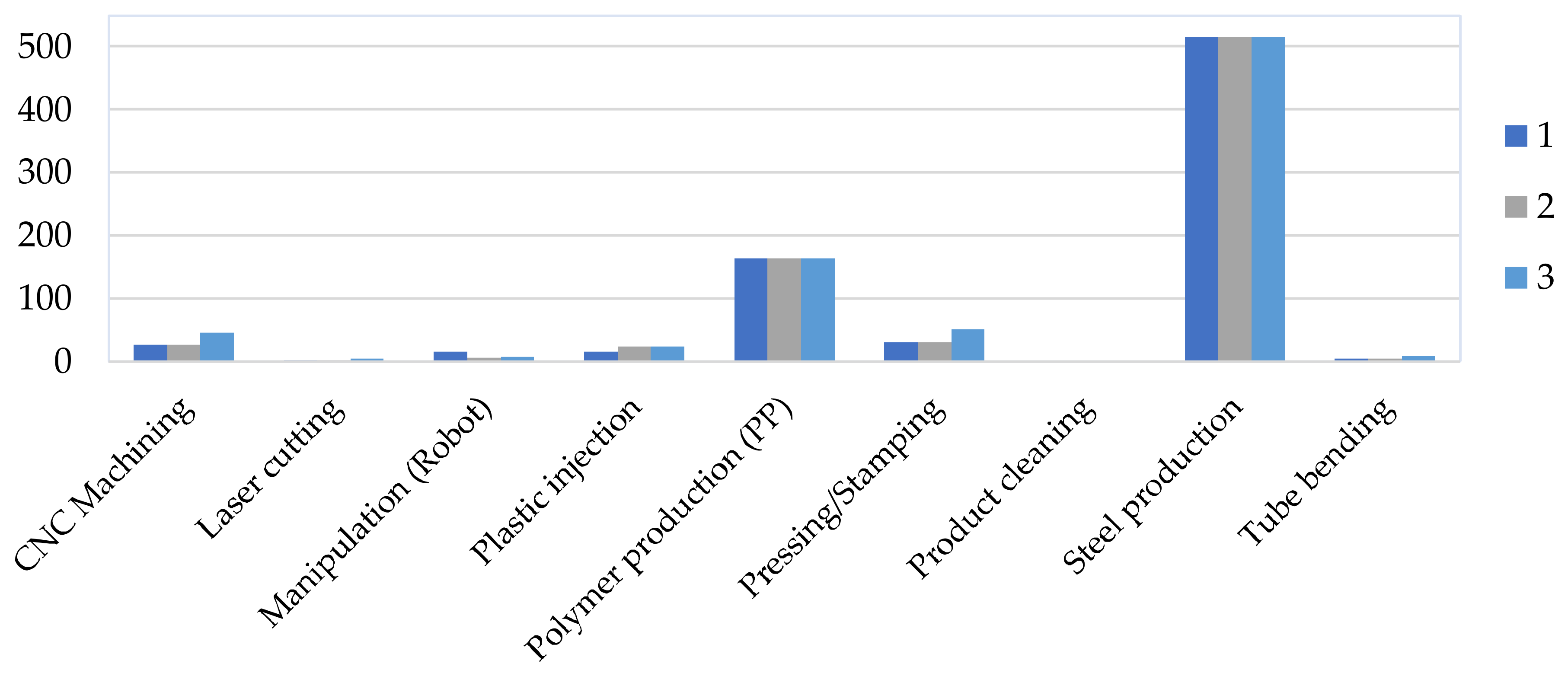
Data analysis as a whole. This means that the CF results for every single equation, applied to all scenarios, will be summed and represented in a single graph (Figure 7) to compare the scenarios with each other and to demonstrate which one possesses or provokes the biggest CF, and thereby the highest pollution and harm toward the environment.
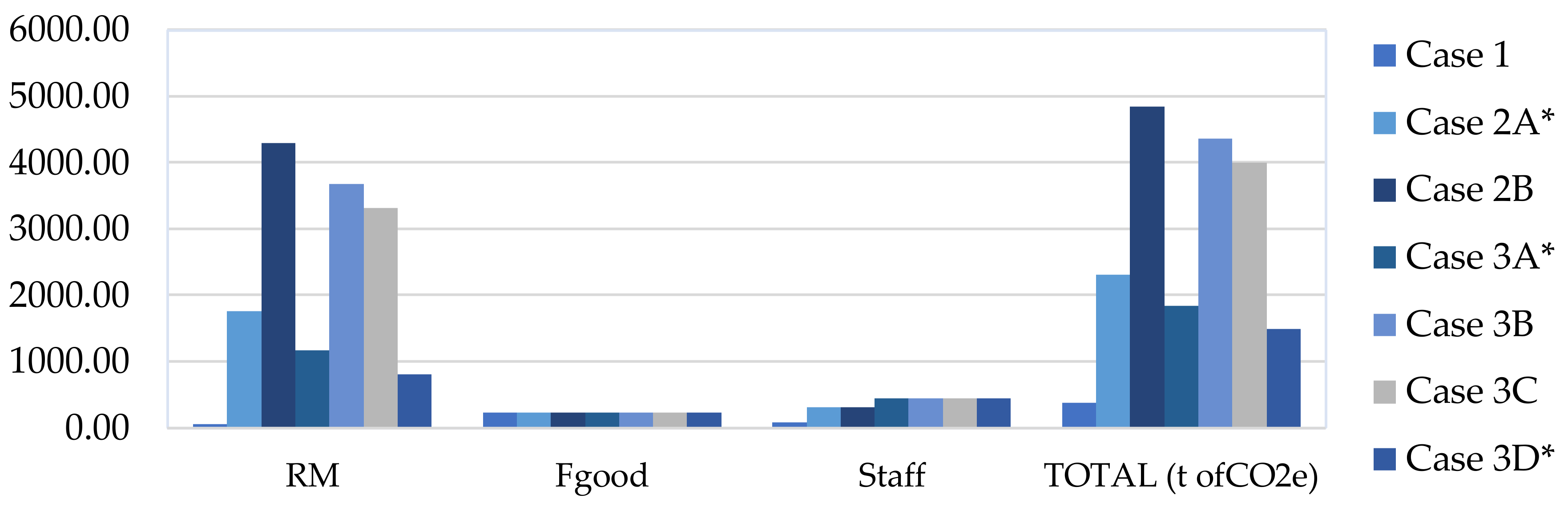
Once the overall CF for each scenario is calculated, it must be broken down into its different contributors in order to classify them according to the percentage of the overall CF for which they are responsible. This allows finding the main contributor or driver of the GHG generation per analyzed scenario.

4.1. Total LCI Results: Environmental Impact Assessment

In Figure 7, the total CO_2e generation per scenario is represented. It is important to emphasize that within each scenario, different variations of the same industrial case have been considered (e.g., A, B, C, and D). The variations themselves correspond to the different transport means that could be considered, especially for goods shipment during the logistics scenario definition. For instance, in Case 3B, part of the goods transport, specifically the raw material (polymer) shipment from China to Germany, was done by airplane, whereas in Case 3D, it was carried out by marine transport.

Comparing the different values represented in Figure 7, the most important takeaway is that the scenario with the widest supply chain (Scenario 3B) would pollute 30.1% more than the industrial case that prioritizes having the suppliers as close as possible to the dispatch area and the sales units (Case 1A) (Table 36).

4.1.1. Boundary Conditions

Goods and Staff Transportation

To understand how and where to start reducing GHG generation, aiming at mitigating the effects of the climate change [88,89], it is indispensable to break down the overall CF per scenario represented in Figure 7 into the different CF sources.

Starting with the influence of the staff and the goods transportation, by comprehending the information illustrated in Figure 8, it is shown that for Case 1 (smallest supply chain—suppliers remaining in a single country), the highest GHG contribution is linked to the final goods dispatch, downstream from the product-manufacturing activities. However, for Scenario 3A, the largest contributor is the raw material (RM), which occurs upstream the final goods production process.

Energy consumption linked to the raw material and part-manufacturing process

Considering that the main energy source used in the production of both the raw material and the final good is electricity, the CF of its production dictates the CF of the total manufacturing process.

As illustrated in Figure 9, although the amount of robots used for Case 1 was higher than those utilized in Scenarios 2 and 3 (Table 24), the total CF for each case remained considerably similar. The root cause of such fact is that the CF of the electricity production in Germany is much lower than that in India (Table 11), and considering that in the third scenario most of the production activities are undertaken in India (Table 5), despite a much lower automation level, the CF of the third scenario’s manufacturing process was higher than the two first cases considered.

Energy transport and storage efficiency

As represented in Figure 10, even if the transport and storage efficiency of the electricity used is assumed to be the same for every machine or process, the energy intensity of the raw material production (polymer and stainless steel) means that the highest GHG contribution in this case is also associated with this field (Figure 10).

4.1.2. Stage 0 and 1: Raw Material and Final Good Production

Besides the information provided above concerning the energy consumption involved in the production of the raw material and final good, it was important to split this CF so that the impact that both may have on the environment could be properly presented and understood. As represented in Table 37, the CF embedded in the raw material production massively exceeded that of the final good.

4.1.3. Stage 2: Product Lifetime Usage

The results represented in Figure 11 clearly explain and justify the current regulations that led the automotive manufacturers to decrease the CF of the vehicles’ utilization [90].

In contrast to the production of the good considered in this paper, its use in the different sorts of vehicles analyzed generated between 1.9 and 3.9 times more CO_2e (Figure 11).

4.1.4. Stage 3: Waste Management

In Figure 12, it is illustrated how the CF varied depending on the waste origin (raw material (“Rmaterial (RM)”), final good manufacturing process (“Mprocess (FG)”) and final good end-of-life (“EOLife FG”)), as well as on the scenario constraints considered.

Due to the larger amount of waste generated during the raw material production compared to that found during the final good manufacturing process (Table 25), the CF of the raw material waste management was substantially higher than that of the manufacturing process (Figure 12).

However, the management of the good itself, once reached its end of life, contained the highest CF overall (Figure 12).

5. Results Interpretation and Discussion

There are three different takeaways or conclusions out of this research that must be emphasized and discussed:

Data analytics: extracting the main CF sources responsible for at least 80% of the GHG emissions and clearing out the influence of the product logistics globalization;
Complexity of the LCI calculations;
Further application of the approach followed in this paper.

5.1. Fields with the Highest GHG Emissions

A very important milestone consisted of extracting, out of the LCI results, the fields whose contribution to the overall CF was the highest. Thus, the total environmental impact of the concerned product industrialization could be mitigated by making the right decisions in the necessary fields.

In this particular case, as represented in Table 38, the biggest contributors to the LCI in terms of CF were first the raw material production, and second the waste disposal.

As one of the main goals of the research, the role of the globalization as a main contributor to the environmental degradation was clearly demonstrated in Case 1, which had the smallest logistics footprint, and generated 30.1% less CO₂ than Case 3B (Table 36), for which a wider supply chain was chosen.

The substantial difference between both cases’ logistics contribution toward the CF can be seen in Table 39.

With all that said, it was clearly proven that the supply chain of a product must be carefully selected, and global logistics might show profitability in terms of pure cost per piece, but once the full environmental impact of the good’s production was taken into account, the negative effect of long-distance shipments was demonstrated. Thus, the supplier panel of a certain industry must not be only based on a cost-effectiveness principle, but also on environmental concerns as well. This means that for a certain project’s industrialization, the project manager must consider the supplier panel based on shipment distance and frequency reduction, as well as on the sustainability actions that the supplier is undertaking (such as improving the transport means used, electrification, etc.).

5.2. Complexity of the LCI Methodology

The major difficulty that such a study presents is in the data collection. In most cases, it is not the size of the data belonging to a certain field, but the immense variety of data sources that need to be managed. Thus, the first immediate finding that the study shows is that even the most accurate LCI will demand certain assumptions.

As a matter of fact, the need to make certain assumptions does not discredit the overall results, as long as it is clearly represented what the level of reliability of the assumptions is.

In this particular paper, there were up to 24 assumptions that were key to providing the results represented in the previous section (Section 4). Each of them was linked to a certain reliability percentage (Table 40). This reliability includes, for instance, considering the assumption of the van weight (Table 40) used to calculate the CF of the product utilization once it is installed in this particular vehicle (Table 35). A 50% reliability implies that the van weight could be 50% higher or lower than the assumption, and thereby the CF of the product use would vary accordingly.

5.3. Further Application of the LCI Method: Life Cycle Assessment (LCA) and Estimate Automation

As stated in the LCA methodology and the related standards [12], once the LCI is available, it must be assessed so that the main purpose, which is to serve as a decision-making tool for the industry [91], is fulfilled.

In this case, the assessment to be done must provide an insight into the items that must be improved in order to reduce the CF, as mandated by the Sustainable Development Goals (SDGs) [85,92,93], and it should also give clear alternatives to the items or features included in the LCI presented in this paper so that a variety of the so-called “greener scenarios” can be added to Table 2.

Moreover, the “greener scenarios” should go hand-in-hand with an economical assessment. Especially considering the initiatives linked to the CO₂ prizing [94], the viability of an alternative green technology must be economically assessed so that the cost of the improvement is compared to the environmental cost, as well as to the economic cost of polluting (CO₂ taxation).

It goes without saying that the industry demands quick reactions, and therefore the LCI and LCA must be provided on time and with the expected quality. Thus, the entire calculator used for this paper needs to be automated by choosing a suitable software so that the time spent looking for reliable databases, structuring the entire business and industrial case, etc., is reduced to the minimum possible.

6. Conclusions

It has been proven that the search for strategies and new technologies to meet the Sustainable Development Goals requires an understanding of the real impact that the production of industrial goods and services causes to the well-being of the environment and living beings [95].

To achieve this level of comprehension within the industry, companies are in need of a suitable methodology that can be easily applied to their day-to-day business, helping to boost sustainable initiatives [96] that will reduce their overall manufacturing footprint and mitigate the impact of CO₂ emissions on the environment wherever it is most efficient and effective [97].

In particular, the environmental impact of the globalization of a product also has been demonstrated, and therefore the application of the LCI method can be considered key to defining the supply chain of a business case while also taking into account what the data that the transportation of goods and employees will mean in terms of product sustainability [98].

Furthermore, the sustainability strategies that most companies commit to follow nowadays [99,100,101,102] also challenge the industry to analyze the viability of a product due to its negative contribution toward the global nature and living beings’ well-being. This analysis aimed to help companies decide which strategy will provide both profit and sustainability.

Thus, this paper serves as an example of the methodology that any company may follow to analyze a CF by focusing on the fields represented in Table 37, and in particular, on the impact of the supply-chain selection on the environment. It is also important to highlight the data that it provides demonstrating the usefulness of the LCA to compare different scenarios in which the same product, along with its life stages, is assessed only by varying the boundary conditions for the concerned scenarios, amongst which the LCA user intends to choose the one that provides the lowest negative environmental impact (Figure 7).

It goes without saying that even if the LCI shows great effectiveness as a decision tool within the industry, there is still much to be improved in order to accelerate the data collection and compilation, as well as to refine the data quality, to be able to obtain the highest reliability in the LCI results, which goes hand-in-hand with having the best LCA.

Author Contributions

Conceptualization, H.J.P.-G. and R.D.; methodology, H.J.P.-G.; formal analysis, H.J.P.-G., R.D.; investigation, H.J.P.-G.; resources, H.J.P.-G., R.D.; writing—original draft preparation, H.J.P.-G.; writing—review and editing, H.J.P.-G., R.D.; supervision, R.D.; funding acquisition, R.D. Both authors have read and agreed to the published version of the manuscript.

Funding

The authors thank the Spanish Ministry of Science, Innovation, and Universities for support through the RTI2018-102215-B-I00 project.

Conflicts of Interest

The authors declare no conflict of interest.

Appendix A

Goods transport CF calculations

Considering utilization of an internal combustion engine vehicle (ICEV):

$C F (k g C O 2 e) = D i s t a n c e (k m) \times G H G f a c t o r (\frac{k g C O 2 e}{k m}) \times T r i p s n u m b e r (-)$

(A1)

$Number of trips = 2 \times \frac{Full load to be transported}{Vehicle load capacity}$

(A2)
Considering the utilization of BEV public transport or another smaller private vehicle:

$C F (k g C O 2 e) = G H G f a c t o r (\frac{k g C O 2 e}{k W h}) \times J o u r n e y c o n s u m p t i o n (k W h) \times N u m b e r o f t r i p s$

(A3)

$N u m b e r o f t r i p s * = 2 \times \frac{F u l l l o a d t o b e t r a n s p o r t e d}{V e h i c l e l o a d c a p a c i t y}$

(A4)

$J o u r n e y c o n s u m p t i o n (k w h) = M e a n p o w e r (k W) \times t r i p d u r a t i o n (h) = M e a n p o w e r (k w) \times \frac{T r i p d i s t a n c e (k m)}{A v e r a g e m e a n s p e e d (\frac{k m}{h})}$

(A5)

* Important to consider the implication of the round trip if the vehicle comes back to the dispatch center empty.

Staff transport CF calculations

Considering utilization of an internal combustion engine vehicle (ICEV):

$C F (k g C O 2 e) = D i s t a n c e (k m) \times G H G f a c t o r (\frac{k g C O 2 e}{k m}) \times N u m b e r o f t r i p s (-) \times N u m b e r o f o p e r a t o r s$

(A6)

$N u m b e r o f t r i p s = 2 \times \frac{A m o u n t o f w o r k i n g h o u r s n e e d e d}{S h i f t d u r a t i o n}$

(A7)
Considering the utilization of BEV public transport or another smaller private vehicle:

$C F (k g C O 2 e) = G H G f a c t o r (\frac{k g C O 2 e}{k W h}) \times J o u r n e y c o n s u m p t i o n (k W h) \times N u m b e r o f t r i p s (-) \times N u m b e r o f o p e r a t o r s \times O p e r a t o r w e i g h t r a t i o (%) / 1000$

(A8)

$N u m b e r o f t r i p s = 2 \times \frac{A m o u n t o f w o r k i n g h o u r s n e e d e d}{S h i f t d u r a t i o n}$

(A9)

$O p e r a t o r w e i g h t r a t i o (%) = \frac{O p e r a t o r a v e r a g e w e i g h t}{T r a n s p o r t m e a n l o a d c a p a c i t y}$

(A10)

$O p e r a t o r w e i g h t r a t i o (%) = \frac{O p e r a t o r a v e r a g e w e i g h t}{T r a n s p o r t m e a n l o a d c a p a c i t y}$

(A11)

* Considering the round trip (from and to the working place) which every operator needs to do every shift.

Energy production and consumption CF calculations

Energy consumption:

$C F (k g C O 2 e) = C o n s u m e d e n e r g y (k w h) \times G H G e n e r g y p r o d u c t i o n (\frac{k g C O 2 e}{k W h})$

(A12)
Energy production:

$C F (k g C O 2 e) = P r o d u c e d e n e r g y (k w) \times G H G u t i l i z e d f o s s i l f u e l (\frac{k g C O 2 e}{k W})$

(A13)

Energy transport and storage CF calculations

Electricity transport (ET):

$C F (k g C O 2 e) = I t e m c o n s u m p t i o n (k w h) \times (1 - \frac{E T e f f i c i e n c y}{100}) \times G H G e l e c t r i c i t y p r o d u c t i o n * (\frac{k g C O 2 e}{k W h})$

(A14)
Electricity storage (ES):

$C F (k g C O 2 e) = I t e m c o n s u m p t i o n (k w h) \times (1 - \frac{E S e f f i c i e n c y}{100}) \times G H G e l e c t r i c i t y p r o d u c t i o n * (\frac{k g C O 2 e}{k W h})$

(A15)

Raw material, intermediate, and final product production CF calculations

Raw material production

$C F (k g C O 2 e) = N u m b e r o f p a r t s (\frac{-}{y e a r}) \times P r o d u c e d m a t e r i a l (k g / p a r t) \times G H G f a c t o r (\frac{k g C O 2 e}{k g o f r a w m a t e r i a l})$

(A16)
Process/machine consumption

$C F (k g C O 2 e) = M a c h i n e o r p r o c e s s p o w e r (k w) \times O p e r a t i n g t i m e (h) \times G H G f a c t o r (\frac{k g C O 2 e}{k w h})$

(A17)

Waste-management CF calculations

Manufacturing process waste (final and intermediate good):

$C F (k g C O 2 e) = N u m b e r o f p a r t s (\frac{-}{y e a r}) \times W a s t e d m a t e r i a l d u r i n g t h e p r o c e s s (k g / p a r t) \times G H G f a c t o r * (\frac{k g C O 2 e}{k g o f w a s t e d m a t e r i a l})$

(A18)

$W a s t e d m a t e r i a l (k g) = P r o d u c e d m a t e r i a l (k g) \times P r o c e s s i n e f f i c i e n c y (%)$

(A19)
Raw material production waste:

$C F (k g C O 2 e) = N u m b e r o f p a r t s (\frac{-}{y e a r}) \times W a s t e d m a t e r i a l (k g / p a r t) \times G H G f a c t o r * (\frac{k g C O 2 e}{k g o f w a s t e d m a t e r i a l})$

(A20)

$W a s t e d m a t e r i a l (k g / p a r t) = \sum_{0}^{i} P r o c e s s e s w a s t e = P r o d u c e d r a w m a t e r i a l (k g) \times (E x t r a c t i o n P r o c e s s i n e f f i c i e n c y (%) + T r e a t m e n t p r o c e s s i n e f f i c i e n c y (%))$

(A21)
Final good end-of-life waste:

$C F (t o f C O 2 e) = \sum_{0}^{i} C O 2 e l i n k e d t o w a s t e d c o m p o n e n t s = N u m b e r o f f i n a l p r o d u c t s (\frac{-}{y e a r}) \times [1 s t C o m p o n e n t w e i g h t (k g) \times G H G f a c t o r * (\frac{k g C O 2 e}{k g o f w a s t e d m a t e r i a l}) + 2 n d C o m p o n e n t w e i g h t (k g) \times G H G f a c t o r * (\frac{k g C O 2 e}{k g o f w a s t e d m a t e r i a l}) + [\dots]$

(A22)

It is crucial to consider each waste-management procedure and the material treated.

Waste-management procedures considered

First, there is the incineration process, which is especially focused on incinerating municipal solid waste (MSW) Equation (A23), (Table A1)) [66].

C F (k g C O 2 e) = I W \times C C W \times F C F \times E F \times \frac{44}{12}

(A23)

Table A1. Variables/factors needed to calculate the GHG generated linked to incineration [93].

Variable	Description	Value
IW	Incinerated MSW volume (kg)
CCW	Proportion of carbon in MSW
FCF	Proportion of mineral carbon content in MSW
EF	Complete combustion intensity of the waste incinerator from MSW (95–99%)	0.975
44/12	CO₂/C molecular weight	3.67

As a second waste-management procedure, there is the so-called “Waste-to-Energy (WtE)”, which basically consists of the incineration of MSW with the intention of recovering energy [83]. The main factors involved in this process are represented in Figure A1.

Figure A1. WtE process description. The graph is based on reference [75].

The third method that was considered was the recycling of every material utilized for the production of the final product.

This particular procedure has shown its utility to be able to use the waste as raw material for manufacturing a new series of product, either of the same kind as the original waste or of a completely different one.

Table A2 highlights the different GHG emissions that the production of raw material provides versus the utilization of recycled waste as renewed raw material for the same aim.

Table A2. Differences between the embodied carbon in the raw material vs. the carbon contained in the recyclable material [82].

Material	Embodied Carbon in Raw Material (kg CO_2e/kg)	Carbon in Recyclable Material	Carbon Emission Reduction by Recycling	In %
General	2.82	0.57	2.25	79.8%
ABS	3.715	0.23	3.485	93.8%
High-density polyethylene (HDPE)	1.31	0.39	0.92	70.2%
LDPE	1.4	0.25	1.15	82.1%
Nylon 6	16.66	0.05	16.61	99.7%
Polypropylene (PP)	5.66	0.59	5.07	89.6%
Expanded polystyrene	2.93	2.55	0.38	13.0%
General-purpose polystyrene	3.25	2.82	0.43	13.2%
Polyurethane	5.45	0.57	4.88	89.5%
Polyethylene terephthalate (PET)	5.7	0.46	5.24	91.9%
PVC (general)	2.23	0.47	1.76	78.9%
PVC pipe	2.5	0.04	2.46	98.4%
Rubber (general)	1.79	0.38	1.41	78.8%

Moreover, there is the process known as landfilling, especially landfilling of MSW, which basically consists of depositing the waste in a certain area, the so-called landfill, in which the waste will remain accumulated and thereby produce CH₄ and CO₂ during its decomposition [98]. The main features and parameters that allow the proper CF estimate (Equation (A24)) of the CH₄ GHG contribution can be seen in Table A3.

C H 4 (t p e r y e a r o r l i f e t i m e) = [(M S W t \times M S W f \times L o) - R] \times (1 - O X)

(A24)

Table A3. Variables/factors needed to calculate the GHG generated linked to landfilling [83].

Variable	Description
MSWt	Total MSW generated
MSWF	Fraction of MSW disposed at the landfill
Lo	Methane generation potential
F	Fraction by volume of CH₄ in landfill gas
R	Recovered CH₄ (Gg/year)
OX	Oxidation factor (fraction)

Final product utilization (item use vs. production) CF calculations

The intention of this analysis consists of comprehending the difference between the GHG emissions embedded in a certain product or component production and those generated during the utilization of the same component.

It goes without saying that the procedure needed for obtaining the CF of the product utilization (Equation (A25)) depends thoroughly on the final use that the product possesses, and whether it will be used on its own or integrated into another system (“mother item”).

In this particular case, the analyzed product is assumed to be a component of a major transport system. For instance: light vehicles (LVEs), heavy-duty transport (HDT), and commercial vehicles (CVEs), amongst others. Thus, the main parameters required to estimate the CF of this component once integrated in the concerned transport system can be observed in Table A4.

Table A4. Variables needed to estimate the CF of the concerned product utilization.

Features	Sort of Vehicle
Life expectancy (km) (A)	LVE, HDT, Light CVE, etc.
Son element weight (g) (B)	LVE, HDT, Light CVE, etc.
Mother element weight (g) (C)	LVE, HDT, Light CVE, etc.
GHG emission (mother element) (kg/km) * (D)	LVE, HDT, Light CVE, etc.
Product weight ratio (%) (E)	LVE, HDT, Light CVE, etc.
Total CO2e caused by the use of the “mother element” (=vehicle) (kg of CO₂) (F)	LVE, HDT, Light CVE, etc.

* Dependent on the fuel utilized by each selected transport mean.

To be able to compare the CF of the product production and its use, it is necessary to establish a weight ratio (E) (Table A4) so that the CO_2e per kg of component versus the CO_2e per kg of the automobile in which the component is assembled and carries its function out can be compared.

C F e m b e d d e d i n t h e p r o d u c t u t i l i z a t i o n (t o f C O 2 e) = E = A \times D \times E = A \times D \times \frac{B}{C}

(A25)

References

Herrmann, C.; Cerdas, F.; Abraham, T.; Büth, L.; Mennenga, M. Biological transformation of manufacturing as a pathway towards environmental sustainability: Calling for systemic thinking. CIRP J. Manuf. Sci. Technol. 2020. [Google Scholar] [CrossRef]
Barry, D.; Hoyne, S. Sustainable measurement indicators to assess impacts of climate change: Implications for the New Green Deal Era. Curr. Opin. Environ. Sci. Health 2021, 22, 100259. [Google Scholar] [CrossRef]
Llopis-Albert, C.; Palacios-Marqu, D.; Sim, V. Fuzzy set qualitative comparative analysis (fsQCA) applied to the adaptation of the automobile industry to meet the emission standards of climate change policies via the deployment of electric vehicles (EVs). Technol. Forecast. Soc. Chang. 2021, 169, 120843. [Google Scholar] [CrossRef]
Barbanera, M.; Castellini, M.; Tasselli, G.; Turchetti, B.; Cotana, F.; Buzzini, P. Prediction of the environmental impacts of yeast biodiesel production from cardoon stalks at industrial scale. Fuel 2021, 283, 118967. [Google Scholar] [CrossRef]
Salvador, R.; Barros, M.V.; dos Santos, G.E.T.; van Mierlo, K.G.; Piekarski, C.M.; de Francisco, A.C. Towards a green and fast production system: Integrating life cycle assessment and value stream mapping for decision making. Environ. Impact Assess. Rev. 2021, 87, 106519. [Google Scholar] [CrossRef]
Kalverkamp, M.; Helmers, E.; Pehlken, A. Impacts of life cycle inventory databases on life cycle assessments: A review by means of a drivetrain case study. J. Clean. Prod. 2020, 269, 121329. [Google Scholar] [CrossRef]
Moro, A.; Lonza, L. Electricity carbon intensity in European Member States: Impacts on GHG emissions of electric vehicles. Transp. Res. Part D Transp. Environ. 2018, 64, 5–14. [Google Scholar] [CrossRef] [PubMed]
Schoeppe, H.; Kleine-Moellhoff, P.; Epple, R. Energy and Material Flows and Carbon Foorprint Assessment Concerning the Production of HMF and Furfural from a Cellulosic Biomass. Processes 2021, 8, 1–12. [Google Scholar]
Ribeiro, J.; Lima, R.; Eckhardt, T.; Paiva, S. Robotic Process Automation and Artificial Intelligence in Industry 4.0—A Literature review. Procedia Comput. Sci. 2021, 181, 51–58. [Google Scholar] [CrossRef]
Aslam, B. Applying environmental Kuznets curve framework to assess the nexus of industry, globalization, and CO₂ emission. Environ. Technol. Innov. 2021, 21, 1–14. [Google Scholar] [CrossRef]
Muthu, S.S. End-of-Life Management of Textile Products. Assessing the Environmental Impact of Textiles and the Clothing Supply Chain; Woodhead Publishing: Swaston, UK, 2014; Volume 157, pp. 143–160. [Google Scholar]
ISO 14040: 2006. 2006 Environmental Management—Life cycle Assessment—Principles and Framework; International Organization for Standardization: Geneva, Switzerland, 2006. [Google Scholar]
Ferrari, A.M.; Volpi, L.; Settembre-Blundo, D.; García-Muiña, F.E. Dynamic life cycle assessment (LCA) integrating life cycle inventory (LCI) and Enterprise resource planning (ERP) in an industry 4.0 environment. J. Clean. Prod. 2021, 286, 125314. [Google Scholar] [CrossRef]
Tisza, M.; Czinege, I. Comparative study of the application of steels and aluminium in lightweight production of automotive parts. Int. J. Light. Mater. Manuf. 2018, 1, 229–238. [Google Scholar] [CrossRef]
Gebler, M.; Cerdas, J.F.; Thiede, S.; Herrmann, C. Life cycle assessment of an automotive factory: Identifying challenges for the decarbonization of automotive production—A case study. J. Clean. Prod. 2020, 270, 122330. [Google Scholar] [CrossRef]
Kashyap, D.; Agarwal, T. Carbon footprint and water footprint of rice and wheat production in Punjab, India. Agric. Syst. 2021, 186, 102959. [Google Scholar] [CrossRef]
Maury, T.; Loubet, P.; Serrano, S.M.; Gallice, A.; Sonnemann, G. Application of environmental life cycle assessment (LCA) within the space sector: A state of the art. Acta Astronaut. 2020, 170, 122–135. [Google Scholar] [CrossRef]
Fathallahi, A.; Coupe, S.J. Life cycle assessment (LCA) and life cycle costing (LCC) of road drainage systems for sustainability evaluation: Quantifying the contribution of different life cycle phases. Sci. Total Environ. 2021, 776, 145937. [Google Scholar] [CrossRef]
Van der Giesen, C.; Cucurachi, S.; Guinée, J.; Kramer, G.J.; Tukker, A. A critical view on the current application of LCA for new technologies and recommendations for improved practice. J. Clean. Prod. 2020, 259, 120904. [Google Scholar] [CrossRef]
Pérez, J.; de Andrés, J.M.; Lumbreras, J.; Rodríguez, E. Evaluating carbon footprint of municipal solid waste treatment: Methodological proposal and application to a case study. J. Clean. Prod. 2018, 205, 419–431. [Google Scholar] [CrossRef]
Suski, P.; Speck, M.; Liedtke, C. Promoting sustainable consumption with LCA—A social practice based perspective. J. Clean. Prod. 2021, 283, 125234. [Google Scholar] [CrossRef]
Wu, Y.; Su, D. LCA of an industrial luminaire using product environmental footprint method. J. Clean. Prod. 2021, 305, 127159. [Google Scholar] [CrossRef]
Ortiz, O.; Castells, F.; Sonnemann, G. Sustainability in the construction industry: A review of recent developments based on LCA. Constr. Build. Mater. 2009, 23, 28–39. [Google Scholar] [CrossRef]
Dal Lago, M.; Corti, D.; Wellsandt, S. Reinterpretring the LCA Standard Procedure for PSS. Procedia CIRP 2017, 64, 73–78. [Google Scholar] [CrossRef]
Falcone, P.M.; Hiete, M.; Sapio, A. Hydrogen economy and sustainable development goals: Review and policy insights. Curr. Opin. Green Sustain. Chem. 2021, 31, 100506. [Google Scholar] [CrossRef]
Campbell, B.M.; Hansen, J.; Rioux, J.; Stirling, C.M.; Twomlow, S.; Wollenberg, E. Urgent action to combat climate change and its impacts (SDG 13): Transforming agriculture and food systems. Curr. Opin. Environ. Sustain. 2018, 34, 13–20. [Google Scholar] [CrossRef]
Papadis, E.; Tsatsaronis, G. Challenges in the decarbonization of the energy sector. Energy 2020, 205, 118025. [Google Scholar] [CrossRef]
Duffner, F.; Mauler, L.; Wentker, M.; Leker, J.; Winter, M. Large-scale automotive battery cell manufacturing: Analyzing strategic and operational effects on manufacturing costs. Int. J. Prod. Econ. 2021, 232, 107982. [Google Scholar] [CrossRef]
Guo, W.; Tian, Q.; Jiang, Z.; Wang, H. A graph-based cost model for supply chain reconfiguration. J. Manuf. Syst. 2018, 48, 55–63. [Google Scholar] [CrossRef]
Almena, A.; Lopez-Quiroga, E.; Fryer, P.; Bakalis, S. Towards the decentralisation of food manufacture: Effect of scale production on economics, carbon footprint and energy demand. Energy Procedia 2019, 161, 182–189. [Google Scholar] [CrossRef]
Schlanbusch, R.D.; Fufa, S.M.; Häkkinen, T.; Vares, S.; Birgisdottir, H.; Ylmén, P. Experiences with LCA in the Nordic Building Industry—Challenges, Needs and Solutions. Energy Procedia 2016, 96, 82–93. [Google Scholar] [CrossRef] [Green Version]
Muthu, S.S. Measuring the Environmental Impact of Textiles in Practice: Calculating the Product Carbon Footprint (PCF) and Life Cycle Assessment (LCA) of Particular Textile Products; Elsevier–Woohead Publishing: Cambridge, MA, USA, 2014; pp. 163–179. [Google Scholar] [CrossRef]
Singh, A.; Mishra, N.; Ali, S.I.; Shukla, N.; Shankar, R. Cloud computing technology: Reducing carbon footprint in beef supply chain. Int. J. Prod. Econ. 2015, 164, 462–471. [Google Scholar] [CrossRef] [Green Version]
Croci, E.; Donelli, M.; Colelli, F. An LCA comparison of last-mile distribution logistics scenarios in Milan and Turin municipalities. Case Stud. Transp. Policy 2021, 9, 181–190. [Google Scholar] [CrossRef]
Vanham, D.; Leip, A.; Galli, A.; Kastner, T.; Bruckner, M.; Uwizeye, A.; van Dijk, K.; Ercin, E.; Dalin, C.; Brandão, M.; et al. Environmental footprint family to address local to planetary sustainability and deliver on the SDGs. Sci. Total Environ. 2019, 693, 133642. [Google Scholar] [CrossRef]
Corominas, L.; Byrne, D.M.; Guest, J.S.; Hospido, A.; Roux, P.; Shaw, A.; Short, M.D. The application of life cycle assessment (LCA) to wastewater treatment: A best practice guide and critical review. Water Res. 2020, 184, 116058. [Google Scholar] [CrossRef]
Buslaev, G.; Morenov, V.; Konyaev, Y.; Kraslawski, A. Reduction of carbon footprint of the production and field transport of high-viscosity oils in the Arctic region. Chem. Eng. Process. Process. Intensif. 2021, 159, 108189. [Google Scholar] [CrossRef]
Skone, T.J.; Curran, M.A. LCAccess—Global Directory of LCI resources. J. Clean. Prod. 2005, 13, 1345–1350. [Google Scholar] [CrossRef]
Yang, Y.; Meng, G. The decoupling effect and driving factors of carbon footprint in megacities: The case study of Xi’an in western China. Sustain. Cities Soc. 2019, 44, 783–792. [Google Scholar] [CrossRef]
Khoo, H.H.; Isoni, V.; Sharratt, P.N. LCI data selection criteria for a multidisciplinary research team: LCA applied to solvents and chemicals. Sustain. Prod. Consum. 2018, 16, 68–87. [Google Scholar] [CrossRef]
Liu, Y.; Li, H.; Huang, S.; An, H.; Santagata, R.; Ulgiati, S. Environmental and economic-related impact assessment of iron and steel production. A call for shared responsibility in global trade. J. Clean. Prod. 2020, 269, 122239. [Google Scholar] [CrossRef]
Xue, Y.-N.; Luan, W.-X.; Wang, H.; Yang, Y.-J. Environmental and economic benefits of carbon emission reduction in animal husbandry via the circular economy: Case study of pig farming in Liaoning, China. J. Clean. Prod. 2019, 238. [Google Scholar] [CrossRef]
Biron, M. The Plastics Industry, Thermosets and Composites, 2nd ed.; Elsevier Ltd: Amsterdam, Oxford, UK, 2014; pp. 1–560. [Google Scholar]
Horvath, C.D. Advanced steels for lightweight automotive structures. In Materials, Design and Manufacturing for Lightweight Vehicles, 2nd ed.; Mallick, P.K., Ed.; Woodhead Publishing: Duxford, UK, 2021; Volume 1, pp. 39–95. [Google Scholar]
Gielen, D.; Boshell, F.; Saygin, D.; Bazilian, M.D.; Wagner, N.; Gorini, R. The role of renewable energy in the global energy transformation. Energy Strat. Rev. 2019, 24, 38–50. [Google Scholar] [CrossRef]
Cuenot, F. CO₂ emissions from new cars and vehicle weight in Europe; How the EU regulation could have been avoided and how to reach it? Energy Policy 2009, 37, 3832–3842. [Google Scholar] [CrossRef]
Krause, J.; Thiel, C.; Tsokolis, D.; Samaras, Z.; Rota, C.; Ward, A.; Prenninger, P.; Coosemans, T.; Neugebauer, S.; Verhoeve, W. EU road vehicle energy consumption and CO₂ emissions by 2050—Expert-based scenarios. Energy Policy 2020, 138, 111224. [Google Scholar] [CrossRef]
Kubáňová, J.; Kubasáková, I.; Dočkalik, M. Analysis of the Vehicle Fleet in the EU with Regard to Emissions Standards. Transp. Res. Procedia 2021, 53, 180–187. [Google Scholar] [CrossRef]
Dinc, A. NOx emissions of turbofan powered unmanned aerial vehicle for complete flight cycle. Chinese J. Aeronaut. 2020, 33, 1683–1691. [Google Scholar] [CrossRef]
Turgut, E.T.; Usanmaz, O.; Cavcar, M. The effect of flight distance on fuel mileage and CO₂ per passenger kilometer. Int. J. Sustain. Transp. 2018, 13, 224–234. [Google Scholar] [CrossRef]
El-Taybany, A.; Moustafa, M.; Mansour, M.; Tawfik, A.A. Quantification of the exhaust emissions from seagoing ships in Suez Canal waterway. Alex. Eng. J. 2019, 58, 19–25. [Google Scholar] [CrossRef]
Kokubun, N.; Ko, K.; Ozaki, M. Cargo conditions of CO₂ in shuttle transport by ship. Energy Procedia 2013, 37, 3160–3167. [Google Scholar] [CrossRef] [Green Version]
Park, N.-K.; Yoon, D.-G.; Park, S.-K. Port Capacity Evaluation Formula for General Cargo. Asian J. Shipp. Logist. 2014, 30, 175–192. [Google Scholar] [CrossRef] [Green Version]
Tran, T.A. Investigate the energy efficiency operation model for bulk carriers based on Simulink/Matlab. J. Ocean Eng. Sci. 2019, 4, 211–226. [Google Scholar] [CrossRef]
Scheepmaker, G.M.; Willeboordse, H.Y.; Hoogenraad, J.H.; Luijt, R.S.; Goverde, R.M. Comparing train driving strategies on multiple key performance indicators. J. Rail Transp. Plan. Manag. 2020, 13, 100163. [Google Scholar] [CrossRef]
Laha, P.; Chakraborty, B. Low carbon electricity system for India in 2030 based on multi-objective multi-criteria assessment. Renew. Sustain. Energy Rev. 2021, 135, 110356. [Google Scholar] [CrossRef]
Liu, H.; Zhang, X.; Quan, L.; Zhang, H. Research on energy consumption of injection molding machine driven by five different types of electro-hydraulic power units. J. Clean. Prod. 2020, 242, 118355. [Google Scholar] [CrossRef]
Meynerts, L.; Brito, J.; Ribeiro, I.; Pecas, P.; Claus, S.; Götze, U. Life Cycle Assessment of a Hybrid Train—Comparison of Different Propulsion Systems. Procedia CIRP 2018, 69, 511–516. [Google Scholar] [CrossRef]
Kawamoto, R.; Mochizuki, H.; Moriguchi, Y.; Nakano, T.; Motohashi, M.; Sakai, Y.; Inaba, A. Estimation of CO₂ Emissions of Internal Combustion Engine Vehicle and Battery Electric Vehicle Using LCA. Sustainability 2019, 11, 2690. [Google Scholar] [CrossRef] [Green Version]
Pizzol, M. Deterministic and stochastic carbon footprint of intermodal ferry and truck freight transport across Scandinavian routes. J. Clean. Prod. 2019, 224, 626–636. [Google Scholar] [CrossRef]
Koj, J.C.; Wulf, C.; Linssen, J.; Schreiber, A.; Zapp, P. Utilisation of excess electricity in different Power-to-Transport chains and their environmental assessment. Transp. Res. Part D Transp. Environ. 2018, 64, 23–35. [Google Scholar] [CrossRef]
Working Days in China. Available online: https://china.workingdays.org/EN/workingdays_holidays_2019.htm (accessed on 14 May 2021).
Working Days in Germany. Available online: https://www.steuergo.de/en/rechner/arbeitstage (accessed on 14 May 2021).
Working Days in India. Available online: https://excelnotes.com/working-days-in-india-in-2019/#:~:text=2019%20%7C%202020,fall%20on%20weekdays%20in%202019 (accessed on 14 May 2021).
Kosai, S.; Yamasue, E. Global warming potential and total material requirement in metal production: Identification of changes in environmental impact through metal substitution. Sci. Total Environ. 2019, 651, 1764–1775. [Google Scholar] [CrossRef]
Liu, Y.; Chen, S.; Chen, A.Y.; Lou, Z. Variations of GHG emission patterns from waste disposal processes in megacity Shanghai from 2005 to 2015. J. Clean. Prod. 2021, 295, 126338. [Google Scholar] [CrossRef]
Baena-Moreno, F.; Cid-Castillo, N.; Arellano-García, H.; Reina, T. Towards emission free steel manufacturing—Exploring the advantages of a CO2 methanation unit to minimize CO₂ emissions. Sci. Total Environ. 2021, 781, 146776. [Google Scholar] [CrossRef]
Song, J.; Jiang, Z.; Ding, Y. Analysisand evaluation of material flow in different steel production processes by gPROMS-based simulation. Energy Procedia 2019, 158, 4218–4223. [Google Scholar] [CrossRef]
Sun, W.; Wang, Q.; Zhou, Y.; Wu, J. Material and energy flows of the iron and steel industry: Status quo, challenges and perspectives. Appl. Energy 2020, 268, 114946. [Google Scholar] [CrossRef]
Kellens, K.; Rodrigues, G.C.; Dewulf, W.; Duflou, J.R. Energy and Resource Efficiency of Laser Cutting Processes. Phys. Procedia 2014, 56, 854–864. [Google Scholar] [CrossRef] [Green Version]
Lin, M.-H.; Renn, J.-C. Design of a Novel Energy Efficient Hydraulic Tube Bender. Procedia Eng. 2014, 79, 555–568. [Google Scholar] [CrossRef] [Green Version]
Meza-García, E.; Rautenstrauch, A.; Bräunig, M.; Kräusel, V.; Landgrebe, D. Energetic evaluation of press hardening processes. Procedia Manuf. 2019, 33, 367–374. [Google Scholar] [CrossRef]
Wirtz, A.; Meißner, M.; Wiederkehr, P.; Biermann, D.; Myrzik, J. Evaluation of cutting processes using geometric physically-based process simulations in view of the electric power consumption of machine tools. Procedia CIRP 2019, 79, 602–607. [Google Scholar] [CrossRef]
Yaskawa. Products. Industrial robots. Available online: https://www.motoman.com/en-us/products/robots/industrial (accessed on 14 May 2021).
Pepe, F. Environmental impact of the disposal of solid by-products from municipal solid waste incineration processes. In Environmental Geochemistry: Site Characterization, Data Analysis and Case Histories; Elsevier: Amsterdam, The Netherlands, 2008; pp. 317–332. [Google Scholar] [CrossRef]
Malakahmad, A.; Abualqumboz, M.S.; Kutty, S.R.M.; Abunama, T.J. Assessment of carbon footprint emissions and environmental concerns of solid waste treatment and disposal techniques; case study of Malaysia. Waste Manag. 2017, 70, 282–292. [Google Scholar] [CrossRef] [PubMed]
De Araújo, J.A.; Schalch, V. Recycling of electric arc furnace (EAF) dust for use in steel making process. J. Mater. Res. Technol. 2014, 3, 274–279. [Google Scholar] [CrossRef] [Green Version]
Cheung, W.M.; Leong, J.T.; Vichare, P. Incorporating lean thinking and life cycle assessment to reduce environmental impacts of plastic injection moulded products. J. Clean. Prod. 2017, 167, 759–775. [Google Scholar] [CrossRef]
Li, X.; Yu, H.; Xue, X. Extraction of Iron from Vanadium Slag Using Pressure Acid Leaching. Procedia Environ. Sci. 2016, 31, 582–588. [Google Scholar] [CrossRef] [Green Version]
EU Population in 2020: Almost 448 million. Available online: https://ec.europa.eu/eurostat/web/products-euro-indicators/-/3-10072020-ap (accessed on 15 May 2021).
Population of Norway. Available online: Tradingeconomics.com (accessed on 16 May 2021).
Devasahayam, S.; Raju, G.B.; Hussain, C.M. Utilization and recycling of end of life plastics for sustainable and clean industrial processes including the iron and steel industry. Mater. Sci. Energy Technol. 2019, 2, 634–646. [Google Scholar] [CrossRef]
Papageorgiou, A.; Barton, J.; Karagiannidis, A. Assessment of the greenhouse effect impact of technologies used for energy recovery from municipal waste: A case for England. J. Environ. Manag. 2009, 90, 2999–3012. [Google Scholar] [CrossRef]
Egüez, A. Compliance with the EU waste hierarchy: A matter of stringency, enforcement, and time. J. Environ. Manag. 2021, 280, 111672. [Google Scholar] [CrossRef]
Cohen, B.; Cowie, A.; Babiker, M.; Leip, A.; Smith, P. Co-benefits and trade-offs of climate change mitigation actions and the Sustainable Development Goals. Sustain. Prod. Consum. 2021, 26, 805–813. [Google Scholar] [CrossRef]
Jigar, E.; Bairu, A.; Gesessew, A. Application of IPCC model for estimation of methane from municipal solid waste landfill. J. Environ. Sci. Water Resour. 2014, 3, 52–58. [Google Scholar]
Hjelkrem, O.A.; Lervåg, K.Y.; Babri, S.; Lu, C.; Södersten, C.-J. A battery electric bus energy consumption model for strategic purposes: Validation of a proposed model structure with data from bus fleets in China and Norway. Transp. Res. Part D Transp. Environ. 2021, 94, 102804. [Google Scholar] [CrossRef]
Azevedo, I.; Leal, V. A new model for ex-post quantification of the effects of local actions for climate change mitigation. Renew. Sustain. Energy Rev. 2021, 143, 110890. [Google Scholar] [CrossRef]
Oh, I.; Wehrmeyer, W.; Mulugetta, Y. Decomposition analysis and mitigation strategies of CO₂ emissions from energy consumption in South Korea. Energy Policy 2010, 38, 364–377. [Google Scholar] [CrossRef]
Morfeldt, J.; Kurland, S.D.; Johansson, D.J. Carbon footprint impacts of banning cars with internal combustion engines. Transp. Res. Part D Transp. Environ. 2021, 95, 102807. [Google Scholar] [CrossRef]
Borghino, N.; Corson, M.; Nitschelm, L.; Wilfart, A.; Fleuet, J.; Moraine, M.; Breland, T.A.; Lescoat, P.; Godinot, O. Contribution of LCA to decision making: A scenario analysis in territorial agricultural production systems. J. Environ. Manag. 2021, 287, 112288. [Google Scholar] [CrossRef]
Halkos, G.; Gkampoura, E.-C. Where do we stand on the 17 Sustainable Development Goals? An overview on progress. Econ. Anal. Policy 2021, 70, 94–122. [Google Scholar] [CrossRef]
Morton, S.; Pencheon, D.; Bickler, G. The sustainable development goals provide an important framework for addressing dangerous climate change and achieving wider public health benefits. Public Health 2019, 174, 65–68. [Google Scholar] [CrossRef]
Cadavid-Giraldo, N.; Velez-Gallego, M.C.; Restrepo-Boland, A. Carbon emissions reduction and financial effects of a cap and tax system on an operating supply chain in the cement sector. J. Clean. Prod. 2020, 275, 122583. [Google Scholar] [CrossRef]
Prado-Galinanes, H.J.; Domingo, R. Impact of the current production, supply and consumption standards on the Sustainable Development Goals. In Proceedings of the IOP Conference Series: Materials Science and Engineering (MSE), Manila, Phillipines, 2021. (In Press). [Google Scholar]
Aguado, S.; Alvarez, R.; Domingo, R. Model of efficient and sustainable improvements in a lean production system through process of environmental innovation. J. Clean. Prod. 2013, 47, 141–148. [Google Scholar] [CrossRef]
Domingo, R.; Marín, M.M.; Claver, J.; Calvo, R. Selection of Cutting Inserts in Dry Machining for Reducing Energy Consumption and CO₂ Emissions. Energies 2015, 8, 13081–13095. [Google Scholar] [CrossRef] [Green Version]
Yang, Y.; Wang, Y. Supplier Selection for the Adoption of Green Innovation in Sustainable Supply Chain Management Practices: A Case of the Chinese Textile Manufacturing Industry. Processes 2020, 8, 717. [Google Scholar] [CrossRef]
Barletta, I.; Despeisse, M.; Hoffenson, S.; Johansson, B. Organisational sustainability readiness: A model and assessment tool for manufacturing companies. J. Clean. Prod. 2021, 284, 125404. [Google Scholar] [CrossRef]
Wolff, S.; Brönner, M.; Held, M.; Lienkamp, M. Transforming automotive companies into sustainability leaders: A concept for managing current challenges. J. Clean. Prod. 2020, 276, 124179. [Google Scholar] [CrossRef]
Trujillo-Gallego, M.; Sarache, W.; Sellitto, M.A. Identification of practices that facilitate manufacturing companies’ environmental collaboration and their influence on sustainable production. Sustain. Prod. Consum. 2021, 27, 1372–1391. [Google Scholar] [CrossRef]
Arrieta, E.M.; González, A.D. Energy and carbon footprints of chicken and pork from intensive production systems in Argentina. Sci. Total Environ. 2019, 673, 20–28. [Google Scholar] [CrossRef]

Figure 1. LCA flow diagram.

Figure 2. Physical appearance of the concerned product: (a) Product composed by a steel body tube and two polymer protections; (b) Product composed by a steel body tube.

Figure 3. Electricity flow from the source to the equipment supplied considering no compensation of the transport and storage inefficiency [61].

Figure 4. Electricity flow from the source to the equipment supplied considering overproduction at the source node to compensate for the transport and storage inefficiency [61].

Figure 5. Polymer production process [57]. Necessary for protecting the product during transport (Table 15).

Figure 7. Total generation of CO_2e per analyzed scenario (kt of CO_2e/production lifetime).

Figure 8. Total CO_2e generated due to the product logistics system, split into the different sorts of goods shipped and the staff commuting.

Figure 9. CF generated during the product-manufacturing process for every scenario/case considered.

Figure 10. Total CO_2e generated depending on the analyzed scenario and on the concerned machine due to the transport and storage of the electricity used (t of CO_2e).

Figure 11. CF of the product during its utilization versus the product’s production CF.

Figure 12. Total CO_2e generated due to waste management (t of CO_2e).

Table 1. Crucial information to create the life cycle inventory. Linked to Figure 1.

1. General Features (Stages 0 and 1—Figure 1)
Production duration (years)	Production volume (parts)	Line capacity (parts/hour)
Operator availability	Sales market	Plant opening time (days/year)
Production footprint	Product description	Product bill of material
2. Material Production and Consumption (Stages 0, 1, and partially 2—Figure 1)
Extracted raw material (kg)	Treated raw material (final) (kg)	Amount of intermediate parts (kg)
Amount of final parts (kg)	Material extraction efficiency (%)	Material treatment efficiency (%)
Material extraction energy consumption (kWh)	Material extraction energy efficiency (%)	Extraction and treatment energy GHG emissions (kg CO_2e/kg material)
3. Logistics Impact (Boundary Condition—Figure 1)
Number of involved countries	Distance between logistic targets (km)	Transport mean used
Transport load capacity (t)	Amount to be loaded (t/year)	Number of trips per year
CO_2e generated (kg/km)	Transport mean power (kW)	Main power source type
Mean average speed (km/h)	Number of operators (-)	Operator average weight (kg)
4. Product Manufacturing Features (Stage 1—Figure 1)
Amount of used machinery (-)	Machinery energy supply (-)	Machinery energy consumption (kWh)
Automation level (-)	Machine efficiency (%)	Emitted GHG (kg CO_2e/kWh)
Number of operators (-)	Machine operating time (h)	Machine power (kW)
5. Energy Production and Consumption (Boundary Condition—Figure 1)
Energy type (-)	Energy production efficiency (%)	Energy mix per considered country (% each source, non-RE vs. RE *)
Energy production GHG generation (kg CO_2e/kWh)	Energy consumption (kWh/km; kg Diesel/km; kWh/Kg; etc.)	Energy generation origin (-)
6. Energy Transport and Storage (Boundary Condition—Figure 1)
Energy transport and storage efficiency (%)	Energy transport and storage system (-)	Sort and amount of transported and stored energy (-) (kW, l, kg, etc.)
7. Process Waste and Final Product EOL (Stages 1 and 3—Figure 1)
Amount of process waste (kg)	Amount of wasted final products (EOL waste) (kg)	Waste management procedures split (%)
Incineration process used (-)	Recycling process used (-)	Waste-to-Energy process (WtE) used (-)
Landfilling process used (-)	Incineration process GHG generation (kg CO_2e/kg of waste)	Recycling process GHG generation (kg CO_2e/kg of waste)
WtE GHG generation (kg CO_2e/kg of waste)	Landfilling GHG generation (kg CO_2e/kg of waste)	Proportion of carbon in MSW (%)
MSW oxidation factor (%)
8. Product Final Use (Stage 2—Figure 1)
Where product will be assembled (-)	GHG of final utilization product (kg CO_2e/Year)	Final utilization product weight (kg)
Final utilization product life expectancy (years)	GHG of final utilization product applied only to the weight of the “son item” analyzed (kg CO_2e/kg)

* RE = renewable energy.

Table 2. Main scenarios that compose the LCI and subsequent LCA.

Main Features	Scenario 1	Scenario 2	Scenario 3
Final good (FG) delivery management	Germany	Germany	Germany
Final good (FG) production	Germany	Germany	India
Raw material extraction	Germany	India and China	India and China
Raw material production	Germany	India and China	India and China
Sales market	EU	EU	EU
Sales volume (parts/year)	2 × 10⁵	2 × 10⁵	2 × 10⁵
Production lifetime (years)	5	5	5
Energy production	Germany	Germany, China, and India (average)	Germany, China, and India (average)
Electrical supply (RE) (% of total)	37.5%	25%	12%
Electrical supply (non-RE) (% of total)	53.9%	43%	56%
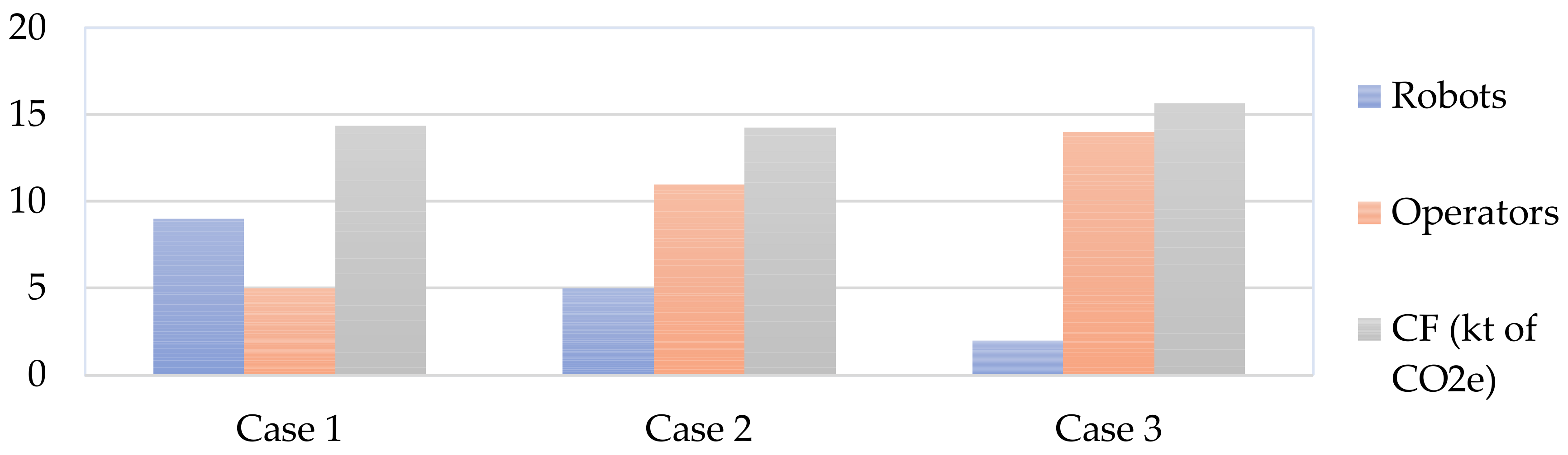
Number of operators (total—including all lines and cells)	5	11	14
Automation level	High (83%)	Medium (50%)	Low (33%)
Number of robots	9	5	2
Number of electrical machines	5	5	5
Number of hydraulic machines	1	1	1
Main used transport means	Road	Sea/road/air	Sea/road/air

Table 3. LCI fields of analysis.

Fields of Analysis
Goods and staff transport
Energy production and consumption
Energy transport and storage
Raw material, intermediate and final product production
Product end-of-Life management (overall waste treatment)
Final product utilization

Table 4. Material composing the final product. These are common materials used in the automotive industry [43,44].

Implied Material	Quantity (g)	Origin
Polymer: polypropylene (PP)	500	Chengdu, China
Polymer: polyethylene terephthalate (PET) *	200	Chengdu, China
Stainless steel: UNS S31640	2500	Pune, India

* Used for the product packaging.

Table 5. Geographical areas where the main industrial activities are carried out.

Industrial Activities	Scenario 1	Scenario 2	Scenario 3
Raw material extraction and processing	Germany	India and China	India and China
Component production	Germany	India and China	India and China
Final good production	Germany	Germany	India
Final good expedition and distribution center	Germany	Germany	Germany

Table 6. Different geographical points that compose the logistic network involved in this product’s production.

Scenario	Variant	Path		Distance (km)	Main Features
1	A	Chengdu	Pune	3330	Air transport
1	B	Chengdu	Pune	4714.48	Road transport: HDT
2	A	Chengdu	Munich	7695.67	Air transport
2	B	Chengdu	Rotterdam	21,742.08	Maritime transport
2	B	Rotterdam	Munich	839.85	Road transport: HDT
3	A	Pune	Munich	6451	Air transport
3	B	Pune	Rotterdam	11,718.22	Maritime transport
3	B	Rotterdam	Munich	839.85	Road transport: HDT
All	All	Munich	Bilbao	1628	Road transport: HDT
All	All	Munich	Porto	2292.8	Road transport: HDT
All	All	Munich	Milan	497.8	Rail transport: train
All	All	Munich	Prague	381.2	Road transport: HDT
All	All	Munich	Krakow	912.27	Road transport: HDT
All	All	Munich	Oslo	1307.05	Air transport
All	All	Munich	Newcastle	1190.52	Air transport
1	All	Cologne	Munich	574.5	Road transport: HDT
1	All	Hamburg	Munich	790.9	Road transport: HDT

Table 11. GHGs generated by electricity generation in each concerned country [56,57,58].

Region	Energy Type	CO_2e	Unit	Comments
Germany	Electricity	686.00	(g/kWh)	Considering generation of CF
India	Electricity	1413.09	(g/kWh)	Considering generation of CF
China	Electricity	893.17	(g/kWh)	Considering generation of CF

Table 12. GHGs emitted by different sorts of fuel used during the overall product life management [57,59,60].

Region	Energy Type	CO_2e	Unit	Comments
Global/General	Gasoline	2280	(g/L of gasoline)	Conventional LVE (gasoline density: 0.720 kg/L) (general combustion)
	Disel_1	2620	(g/L of diesel)	Conventional LVE (diesel density: 0.850 kg/L) (general combustion)
	Diesel_2	3150	(g/L of diesel)	Marine diesel (general combustion)
	Coal_1	2700	(g/kg of coal)	Generation of CF
	Coal_2	900	(g/kWh)	Generation of CF

Table 13. Electricity storage and transport efficiency [61].

Feature	Energy Type	Efficiency Factor (%)
Storage	Electricity	96
Transport	Electricity	94.5

Table 26. Amount of raw material to be treated considering the final product weight and the inefficiencies registered for each process used (Table 25).

Used Materials	Final Amount Needed (g)	Compensation Due to the Process Inefficiency (%)	Needed Raw Material (g)
Polypropylene (PP)	500	5.41%	527.06
Polyethylene terephthalate (PET)	200	5.41%	210.82
Stainless steel: UNS S31640	2500	97.30%	4932.5

Table 27. Total process waste (kg) per material type by the end of the product lifetime production.

PP	PET	Stainless Steel
27,050	10,820	2,307,500

Table 28. Total product EOL waste per material type.

PP	PET	Stainless Steel
500,000	200,000	2,500,000

Table 29. Waste split according to the sales market and the material that composes the product as well as its packaging [80,81].

Country	Population (Millions of Inhabitants)	Product Market Share (%)	Product EOL Waste per Country (kg)
Country	Population (Millions of Inhabitants)	Product Market Share (%)	PP	UNS S31640	PET
Germany	83.1	26%	128,846	644,228	51,538
Spain	47.1	15%	73,028	365,140	29,211
Portugal	10.3	3%	15,970	79,850	6388
Czech	10.7	3%	16,590	82,951	6636
Italy	60.3	19%	93,494	467,472	37,398
Poland	38.4	12%	59,539	297,694	23,816
Norway	5.319	2%	8247	41,235	3299
UK	67.26	21%	104,286	521,429	41,714

Table 30. Plastic waste split depending on the country and the management strategy or process chosen [83,84,85].

Country	Pure Incineration	No Proper Treatment	Recycling	Energy Recovery	Landfilling
Germany	0%	0%	38.6%	60.6%	0.8%
UK	0%	0%	32.1%	38.3%	29.6%
Italy	0%	0%	29.0%	33.8%	37.2%
Spain	0%	0%	36.5%	17.1%	46.4%
Poland	0%	0%	26.8%	29.1%	44.1%
Czechia	0%	0%	38.0%	23.0%	39.0%
Portugal	0%	0%	37.0%	33.0%	30.0%
Norway	0%	0%	42.0%	56.0%	2.0%
China	12%	17%	29%	0%	42.0%
India	35%	0%	20.0%	0.0%	35.0%

Table 31. Total municipal solid waste (MSW) split depending on the country and the management strategy or process chosen [66,84,85].

Country	Landfilling	Incineration	WtE	Recycling
Germany	13	5	21	61
UK	37	9	6	48
Italy	22	7	5	66
Spain	43.5	0	6.5	50
Poland	31	1	7	61
Czechia	35	0	9	56
Portugal	39.5	0.5	17	43
Norway	31 *	26 *	0 *	43*
China	72.9	15.3	No data	No data
India	**	**	**	**

* Replaced by the statistics of the EU. Assumed to be comparable and due to lack of specific and convincing data related to the waste management in Norway. ** Due to unavailability of data, it is assumed that 30% of the steel is recycled in India, and the rest (70%) is 90% landfilled and 10% incinerated.

Table 32. PP waste-management technologies used [66,82,83].

Waste-Management Strategy	PP
Waste-Management Strategy	Method	GHG Contribution
Incineration	Mass burn incineration (MBI)—IPCC calculation	Equation (A23) (Appendix A)
Landfilling	IPCC method	Equation (A24) (Appendix A)
WtE	NA	NA
Recycling	Feedstock of plastic in blast furnace (BF)	0.59 (kg CO_2e/kg of PP)

Table 33. PET waste-management technologies used [66,82,86].

Waste-Management Strategy	PET
Waste-Management Strategy	Method	GHG Contribution
Incineration	Mass burn incineration (MBI)—IPCC calculation	Equation (A23) (Appendix A)
Landfilling	IPCC method	Equation (A24) (Appendix A)
WtE	NA	NA
Recycling	Feedstock of plastic in blast furnace (BF)	0.46 (kg CO_2e/kg of PET)

Table 34. Stainless steel waste-management technologies used [66,85,86].

Waste-Management Strategy	UNS S31640
Waste-Management Strategy	Method	GHG Contribution
Incineration	Mass burn incineration (MBI)—IPCC calculation	Equation (A23) (Appendix A)
Landfilling	Direct reduced iron (coal)—electric arc furnace without added steel scrap	3.2 (kg CO_2e/kg of steel)
WtE	NA	NA
Recycling	Direct reduced iron (gas)—electric arc furnace with 400 kg of steel scrap added to the process	1.16 (kg CO_2e/kg of steel)

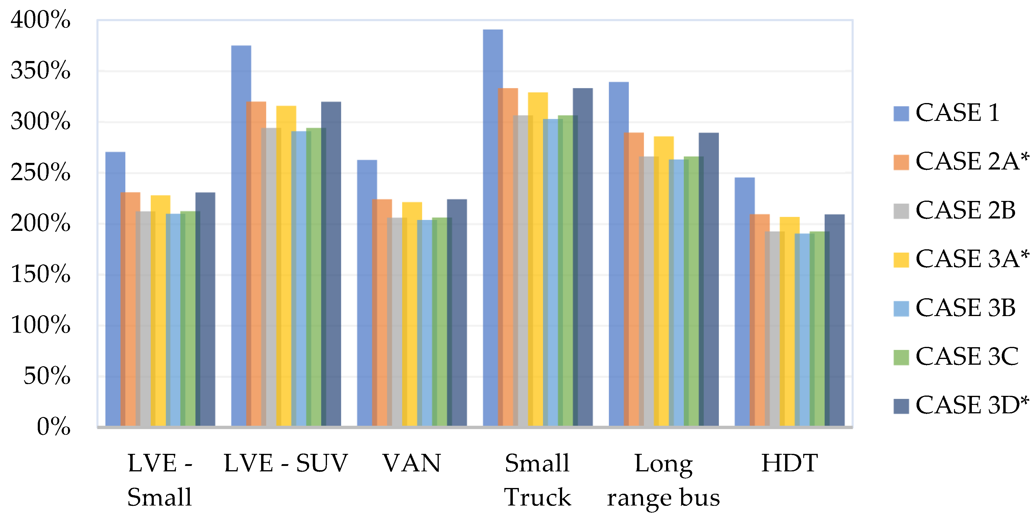
Table 35. Main features of the analyzed product that are necessary to calculate the CF of the product once assembled and used in the final assembly/vehicle [46,47,48,87].

Features	Sort of Vehicle
Features	Small LVE	LVE—SUV	VAN	LCV ¹	Long Range Bus	HDT ²
Life expectancy (km)	200,000 *	200,000 *	200,000 *	500,000 *	500,000 *	500,000 *
Son element weight (g)	3200	3200	3200	3200	3200	3200
Mother element weight (g)	1,300,000	1,480,000	2,500,000 *	7,500,000	13,210,000 *	18,000,000
GHG emission (mother element) (kg/km)	135	213	252	450	688	678
Product weight ratio (%)	0.32%	0.21%	0.13%	0.05%	0.03%	0.02%
Total CO₂e caused by the use of the mother element (=vehicle) (kg of CO₂)	27,000	42,600	50,400	225,000	344,000	339,000

* Assumption; ¹ light commercial vehicle; ² heavy-duty truck.

Table 36. Most centralized production compared to the most globalized scenario. CF measured in CO_2e.

Simplified LCA Assessment—CO_2e Generation (CF)
Best case	1	Base
Worst case	3B	+30.1%

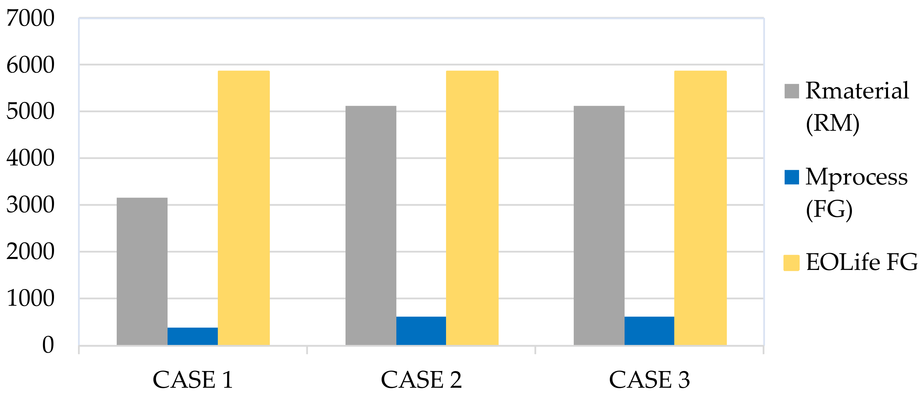
Table 37. CF differentiating the raw material production from the production of the good.

	Raw Material Production (kt of CO_2e)	Final Good Production (kt of CO_2e)
Case 1	12.68	1.67
Case 2	12.78	1.49
Case 3	12.78	2.90

Table 38. Segregation and classification of the overall CF into the different industrial fields that compose every item in production.

	Product Production and Energy use (Boundary, Stages 0 and 1)		Energy Transport and Storage (Boundary Condition)		Waste Disposal (Stage 3)		Transport (Boundary Condition)
	Raw Material	Final Good	Transport	Storage	EOL	Production	Goods	Staff
Case 1	49.53%	8.00%	3.176%	0.008%	23.511%	14.224%	1.191%	0.36%
Case 2A	42.70%	6.64%	2.738%	0.018%	20.270%	19.880%	6.894%	0.87%
Case 3A	41.27%	11.11%	2.913%	0.024%	19.593%	19.216%	4.689%	1.18%
Case 2B	39.26%	6.10%	2.518%	0.017%	18.639%	18.281%	14.385%	0.80%
Case 3B	38.08%	10.25%	2.688%	0.022%	18.075%	17.728%	12.071%	1.09%
Case 3D	41.77%	11.24%	2.949%	0.024%	19.831%	19.450%	3.530%	1.20%
Case 3C	38.50%	10.36%	2.718%	0.022%	18.278%	17.927%	11.085%	1.10%

Table 39. Logistics CF of Case/Scenario 1 vs. Case/Scenario 3B.

Transport (t CO₂)
Case	Short Description	Goods	Employees
Case 1	Smallest logistics footprint	297.02	89.68
Case 3B	Widest supply chain	3916.93	354.57

Table 40. Main assumptions used to complete the CF estimate linked to the expected reliability level presumed. Important to consider that the Reliability (%) is just a rough estimate based on the sort of missing data and/or the data sources found.

Field	Assumption	Reliability
Transport of goods	If the total weight to be shipped is lower than the transport mean capacity, the CF calculated only considers the CO_2e linked to the weight of the goods shipped and not the CF of the full vehicle	80%
Transport of goods	The return for each transport mean is not considered as a source of CO_2e	75%
Transport of staff	Average speed of a train = 130 km/h	75%
Energy transport and storage	It is considered that the energy is stored in a machine as long as there is a battery. Thus, for regular electrical machines, it is considered only the electrical energy performance (95%)	75%
Energy transport and storage	Efficiency considered the same for all sorts of machines used	50%
Lifetime product use	Weight of a VAN is assumed to be 2.5 tonnes	60%
Lifetime product use	Life expectancy of each vehicle (certain amount of km per transport mean)	75%
RM production	Polymer is produced in China for Cases 2 and 3	50%
RM production	Steel is produced in India for Cases 2 and 3	50%
Manufacturing processes	It is considered that the main energy source is electricity	80%
Cargo train	If the max speed is 95 km/h, the average speed is considered to be 80 km/h	75%
Minerals extraction for steel production	Efficiency considered to be around 76%	90%
Casting (steel) and plastic pellet production	It is considered that the efficiency of these two processes is 95%	60%
Metal forming and cutting	It is considered to have an efficiency of 90%, which leaves 10% of the material as waste	60%
Pressing and stamping	Process/machine considered to be electric	75%
Press used	Power considered to be 50 kW	40%
Product-cleaning process	Considered to be a manual process—no energy implied during the action	50%
Plastic incineration CF	Proportion of carbon in MSW (FCF) considered to be 1	80%
Landfilling CF	Degradable organic carbon (DOC) is considered to be 0.15 (kg of C/kg SW)	95%
Landfilling CF	Fraction of DOC (DOCF) dissimilated is considered to be 0.77	95%
Steel waste management in the European market	In absence of data, it is considered that the steel waste-management split is according to the overall MSW split in the concerned country	35%
Waste management—India	It is assumed that 30% of the steel is recycled in India and the rest is 90% to landfilling and 10% to energy recovery/incineration	20%
Steel CF calculation	If the steel is not recycled, the waste-management process used is the “direct reduced iron (coal)—electric arc furnace” with a CF of (3.2 kg CO_2e/kg material) without scrap added. However, if the steel is recycled, the process used is the “direct reduced iron (gas)—electric arc furnace with 400 kg of scrap steel added to the process”, this having a CF of 1.16 kg CO_2e/kg of product	30%
MSW in Norway	Waste-management split assumed to be the same as the average in the EU	60%

Publisher’s Note: MDPI stays neutral with regard to jurisdictional claims in published maps and institutional affiliations.

© 2021 by the authors. Licensee MDPI, Basel, Switzerland. This article is an open access article distributed under the terms and conditions of the Creative Commons Attribution (CC BY) license (https://creativecommons.org/licenses/by/4.0/).

Share and Cite

MDPI and ACS Style

Prado-Galiñanes, H.J.; Domingo, R. Quantifying the Impact of Production Globalization through Application of the Life Cycle Inventory Methodology and Its Influence on Decision Making in Industry. Processes 2021, 9, 1271. https://doi.org/10.3390/pr9081271

AMA Style

Prado-Galiñanes HJ, Domingo R. Quantifying the Impact of Production Globalization through Application of the Life Cycle Inventory Methodology and Its Influence on Decision Making in Industry. Processes. 2021; 9(8):1271. https://doi.org/10.3390/pr9081271

Chicago/Turabian Style

Prado-Galiñanes, Humberto. J., and Rosario Domingo. 2021. "Quantifying the Impact of Production Globalization through Application of the Life Cycle Inventory Methodology and Its Influence on Decision Making in Industry" Processes 9, no. 8: 1271. https://doi.org/10.3390/pr9081271

Note that from the first issue of 2016, this journal uses article numbers instead of page numbers. See further details here.

Article Menu

Quantifying the Impact of Production Globalization through Application of the Life Cycle Inventory Methodology and Its Influence on Decision Making in Industry

Abstract

1. Introduction

1.1. Motivation to Research and Create This Paper

1.2. Main Hypothesis, Assumptions and Considerations of the Article

1.3. Article Structure

1.4. Veracity of the Database amd Countermeasures: Uncertainty Assessment

1.5. Anticipated Results

2. Literature Review

3. Materials and Methods

3.1. Goal and Scope Definition

LCA Process Flow Diagram

3.2. Inventory Analysis

3.2.1. Equations Applied for Each Analyzed Field in Order to Calculate Their CF

3.2.2. LCI Input Applied to the Scenarios Considered in the Paper

Product Features Considered in the LCI: Real Data as Well as Assumptions

Goods and Staff Transport

Energy Production and Consumption

Energy Transport and Storage Efficiency

Raw Material, Intermediate, and Final Product Production

Product End-of-Life Management (Overall Waste Treatment)

Final Product Utilization (Item Use vs. Production)

3.3. Functional Unit

4. Results

4.1. Total LCI Results: Environmental Impact Assessment

4.1.1. Boundary Conditions

4.1.2. Stage 0 and 1: Raw Material and Final Good Production

4.1.3. Stage 2: Product Lifetime Usage

4.1.4. Stage 3: Waste Management

5. Results Interpretation and Discussion

5.1. Fields with the Highest GHG Emissions

5.2. Complexity of the LCI Methodology

5.3. Further Application of the LCI Method: Life Cycle Assessment (LCA) and Estimate Automation

6. Conclusions

Author Contributions

Funding

Conflicts of Interest

Appendix A

References

Share and Cite

Article Metrics

Article Access Statistics

Further Information

Guidelines

MDPI Initiatives

Follow MDPI