
Frequency and Characteristics of Inland Advecting Sea Breezes in the Southeast United States
by
 ,
,
Brian Viner
1,*, 
Stephen Noble
1,
Jian-Hua Qian
1,
David Werth
1,
Paul Gayes
2,
Len Pietrafesa
3 and
Shaowu Bao
2 
1
Atmospheric Technologies Group, Savannah River National Laboratory, Aiken, SC 29829, USA
2
Department of Coastal and Marine Systems Science, Coastal Carolina University, Conway, SC 29528, USA
3
Department of Marine, Earth and Atmospheric Sciences, North Carolina State University, Raleigh, NC 27695, USA
*
Author to whom correspondence should be addressed.
Atmosphere 2021, 12(8), 950; https://doi.org/10.3390/atmos12080950
Submission received: 22 June 2021
/
Revised: 15 July 2021
/
Accepted: 20 July 2021
/
Published: 23 July 2021
(This article belongs to the Section Biosphere/Hydrosphere/Land–Atmosphere Interactions)
Abstract
:Sea breezes have been observed to move inland over 100 km. These airmasses can be markedly different from regional airmasses, creating a shallow layer with differences in humidity, wind, temperature and aerosol characteristics. To understand their influence on boundary layer and cloud development on subsequent days, we identify their frequency and characteristics. We visually identified sea breeze fronts on radar passing over the Savannah River Site (SRS) between March and October during 2015–2019. The SRS is ~150 km from the nearest coastal location; therefore, our detection suggests further inland penetration. We also identified periods when sea breeze fronts may have passed but were not visually observed on radar due to the shallow sea breeze airmass remaining below the radar beam elevation that ranges between approximately 1–8 km depending on the beam angle and radar source (Columbia, SC or Charleston, SC). Near-surface atmospheric measurements indicate that the dew point temperature increases, the air temperature decreases, the variation in wind direction decreases and the aerosol size increases after sea breeze frontal passage. A synoptic classification procedure also identified that inland moving sea breezes are more commonly observed when the synoptic conditions include weak to moderate offshore winds with an average of 35 inland sea breezes occurring each year, focused primarily in the months of April, May and June.
1. Introduction
Coastal regions are impacted by sea breeze circulations driven by thermal differences between the ocean and land. In the southeast United States, the coastal region is characterized by a long coastline extending thousands of miles along the Gulf of Mexico, around the Florida peninsula and extending northward along the Atlantic Ocean. The waters of the Gulf of Mexico and the Gulf Stream moving northward along the western Atlantic Ocean tend to be particularly warm, while the inland regions are generally characterized by a flat coastal plain covered in a range of coastal wetlands, forests and agricultural regions. Generally flat topography means that there are no topographical hinderances to sea-breeze-related airmasses moving inland, unlike in the western United States, where large coastal hills and mountains can limit the inland transport of a sea breeze airmass in many places.
Sea breeze circulations can impact regions far from the coast depending on the strength of the circulation and other regional atmospheric conditions. Sea breeze fronts have been observed to travel inland as a transient gravity current that persists even after being cut-off from the initial coastal circulation [1,2]. In regions characterized by mountainous or complex coastlines, the inland travel of sea breezes may be limited to 30–40 km [3,4], but in regions that are broadly flat with onshore prevailing winds, they can be observed to push to 80–100 km inland with regularity [2,5]. The movement of sea breezes inland can bring a distinct airmass with atmospheric properties and aerosol characteristics relative to the prevailing airmass over a region.
Given the prevalence of aerosol formation near the surface, a modified surface environment would be expected to affect the generation and growth of aerosols as well as the formation of secondary particles. Prior work has yielded measurements that show how the source of an airmass has significant impacts on the distribution of cloud condensation nuclei (CCN) and subsequent cloud microphysical properties [6] for both maritime [7] and continental airmasses [8]. Additionally, variations in atmospheric aerosol concentrations lead to differences in the type and rate of precipitation that occurs from deep convective clouds [9,10]. This suggests that accurate modeling of the frequency of sea breezes may be an important component for simulating the formation of aerosols and clouds in coastal regions and for regions some distance inland.
A complicating factor in studying sea breezes over long time scales is that numerical models tend to have difficulty resolving them due to their limited horizontal extent and the local gradients that drive their formation, often requiring a coupled Large-Eddy Simulation model to more accurately predict them [11]. Horizontal grid resolutions, particularly of regional-scale earth system models, are improving, but will still have difficulty accurately capturing the onset and inland intrusion of the sea breeze. Equally important in modeling sea breezes is the vertical grid spacing, which may need to be quite fine near the surface due to the shallow nature of sea breezes.
This study is designed to identify the frequency of intruding sea breezes at the Savannah River Site, Aiken, SC, which is located approximately 150 km inland near the edge of the coastal plain. In the southeast United States, a large portion of the region is classified as coastal plain due to the presence of the Atlantic Ocean and the Gulf of Mexico, and it is a region where inland moving sea breezes have been identified in the region previously [1]. The region is broadly characterized with forested regions that play a role in the development of the formation of aerosols through their release of biogenic volatile organic compounds.
The significance of the work lies in developing a basis for understanding the frequency with which sea breezes may influence the development of clouds by modifying the surface layer. While the presence of inland advecting sea breezes has been identified in previous studies, there has been little work to understand whether this is an isolated phenomena or a regularly occurring weather pattern that can influence the climatological characteristics of an inland region apart from the synoptic forcing.
It is expected that the development of such a climatology can lend itself to identifying key contributors that determine the extent of the inland movement of sea breezes as well as capture the expected conditions following a sea breeze passage at the Savannah River Site. While the specific characteristics that affect the sea breeze and the conditions following the sea breeze passage are likely to exhibit variation with geographic location, this study establishes the characteristics of inland sea breezes, including their frequency, general atmospheric properties and identification of signals representative of the sea breeze, in order to provide a basis for comparison in future studies of sea breezes in other regions.
2. Materials and Methods
2.1. Identifying Sea Breezes
Sea breeze signals can be masked within larger synoptic flows or exhibit signals similar to a frontal passage or other change in airmass properties. For those reasons, we used radar to perform an initial examination of the frequency of sea breezes. This provides us with a set of days from which we can examine the expected changes in meteorological variables that result from a sea breeze passing over an inland region. Once those characteristics have been identified, we can then rely on surface-based measurements to identify the potential frequency of inland advecting sea breezes.
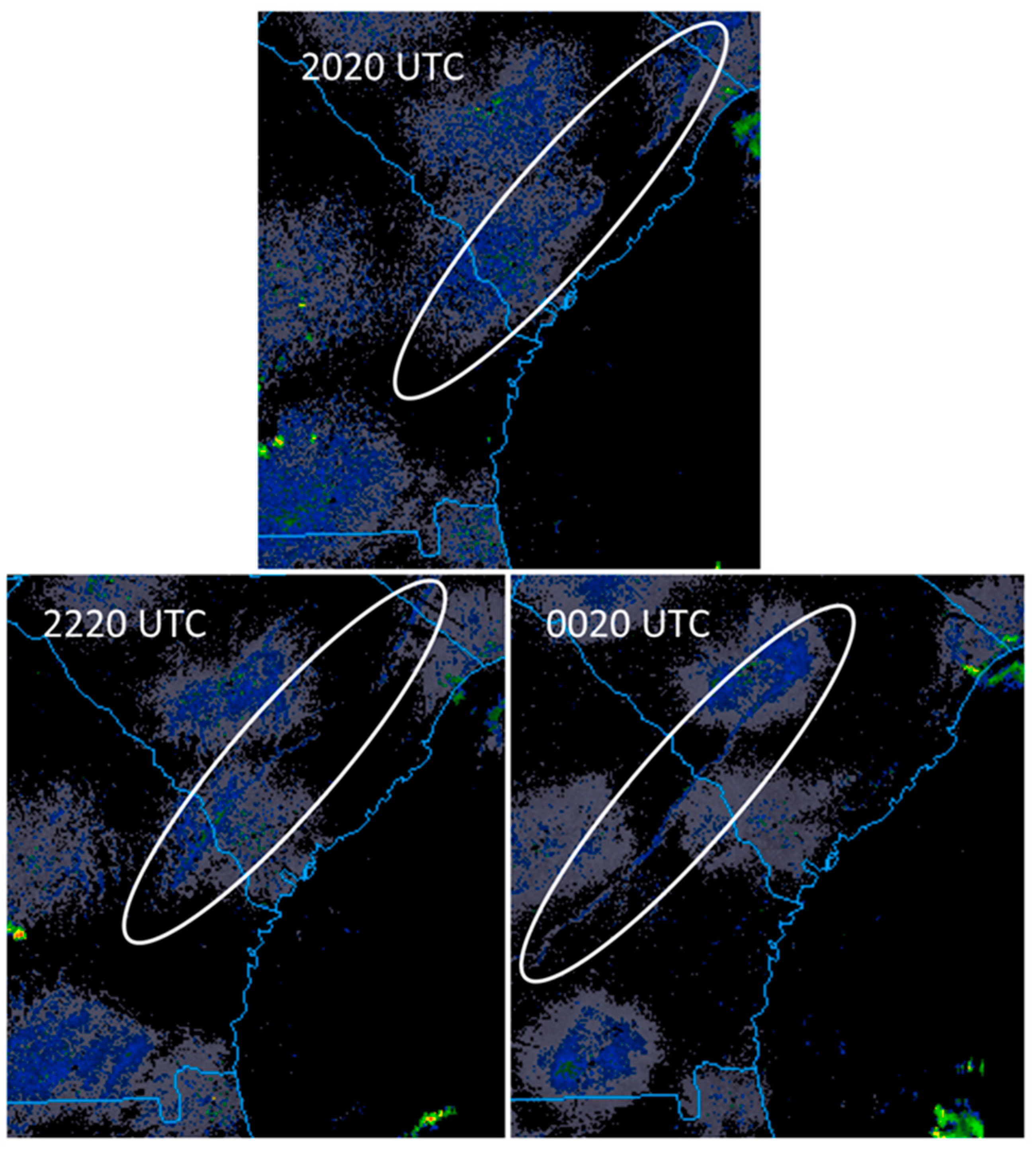
Dates with inland-moving sea breezes were identified using visual analysis of radar images during the months of March–October in 2015–2019. The sea breeze creates a localized radar signature due to the density differences between the air over a location and the advancing sea breeze air mass illustrated in Figure 1. Dates were recorded where there was visual evidence of a sea breeze passing over the SRS. We expect that this does not represent a fully comprehensive set of sea breezes passing over the region due to complicating factors that prevented a clear analysis on many days. The first factor was thunderstorm or precipitation in the area, which would obscure the sea breeze signal. We did not specifically dismiss cases where rain was occurring in the region, but in most cases, it was difficult to tell if the signals being observed on radar were due to a sea breeze or some other phenomenon such as a gust front or weak reflectivity in the radar signature from low precipitation. The second factor occurred when a sea breeze front signal was lost from radar due to its shallow nature, which was contained below the radar beam elevation that ranges between approximately 1–8 km depending on the beam angle and radar source (Columbia, SC, USA or Charleston, SC, USA). In these cases, we did not include the date nor data in our analysis because we could not confirm that the sea breeze reached the SRS.
2.2. Meteorological Measurements
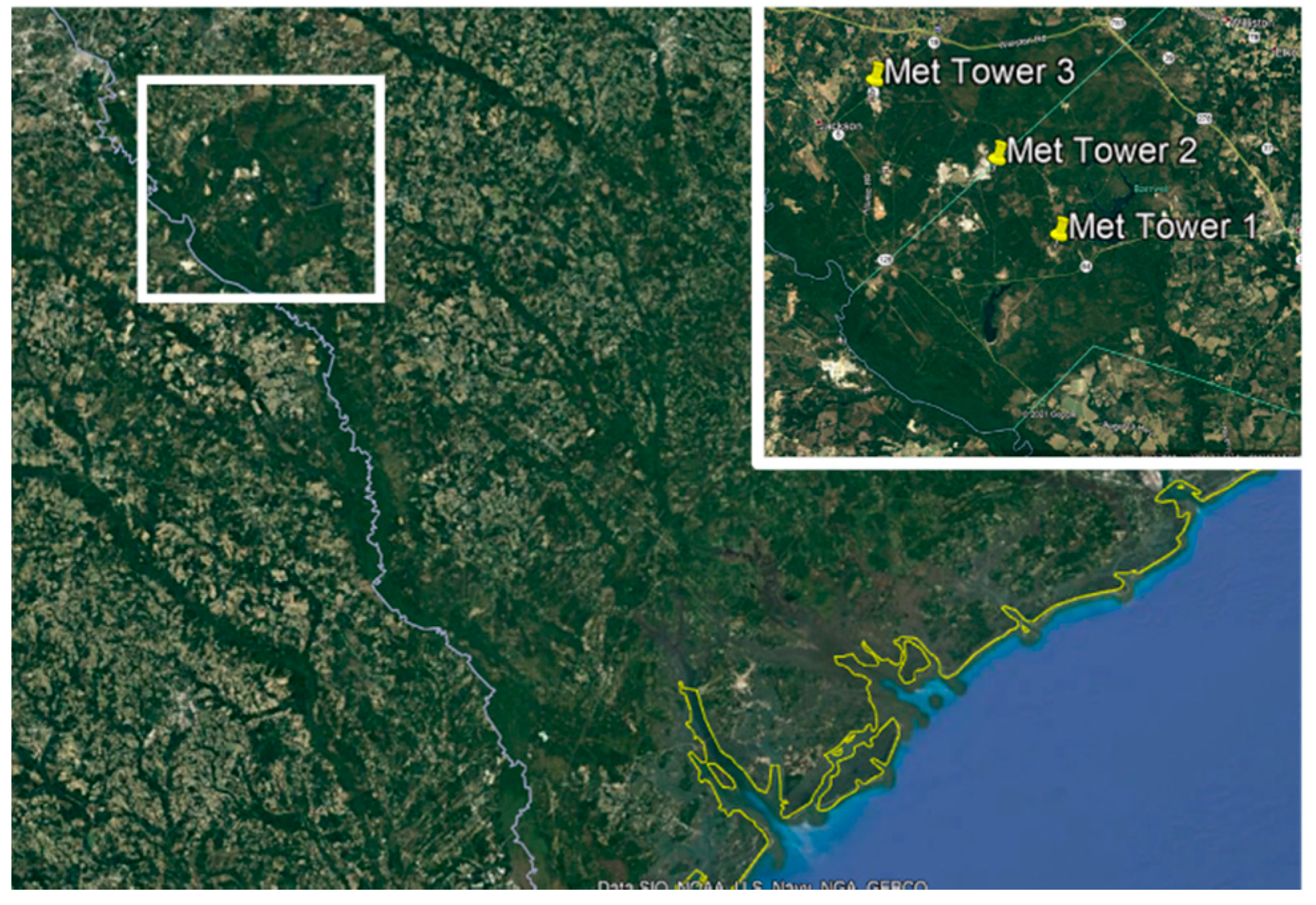
Measurements were taken at the SRS, which maintains a network of 61 m towers instrumented with RM Young 81,000 sonic anemometers and RM Young 41382VC temperature/RH probes providing humidity, temperature and wind measurements that are averaged at 15-min intervals and were used to identify the arrival of the sea breeze over the SRS. Three towers were selected from the SRS network (identified as Met Tower 1, 2 and 3 in the inset in Figure 2, henceforth abbreviated as MT1, MT2 and MT3), which provided a transect across the SRS that was perpendicular to the coast and the expected direction of sea breeze front movement. The purpose of this transect was to identify a time-series of meteorological data that could detail the movement and change of the associated meteorological parameters at each tower in succession. The distance from the coast ranged from ~140 km for MT1 to ~160 km for MT3. Data for the meteorological tower network has undergone quality assurance checks [12].
Aerosol characteristics are estimated using a Vaisala CL31 ceilometer (910 nm) deployed at the SRS. Based on the measurements of the two-way attenuated backscattered energy, we can estimate changes in the air mass as a result of the sea breeze. While the changes cannot be specifically identified based on the backscatter measurements alone, an increase in backscatter would be attributable to either an increase in aerosol size or concentration. For the purpose of this study, the specific changes are not the focus, but rather an identification that the aerosol properties of the atmosphere do change following the passing of a sea breeze front and identifying for how long they may persist.
2.3. Synoptic Pattern Classification
To analyze whether the frequency of inland moving sea breezes is affected by ambient synoptic atmospheric conditions, we classified daily weather types by a K-Means clustering method using 850 hPa winds of the National Center for Environmental Prediction (NCEP) reanalysis data over the domain of (100° W–65° W, 20° N–45° N) as in [13] and as used for weather and climate studies in southeast Asia [14,15,16] and northeast U.S. [17]. Using the 850 hPa winds allows for a broad analysis that is not heavily affected by small-scale topographically influenced surface measurements and, therefore, results in a smoother analysis. The purpose of the analysis is to identify general weather patterns over the region in terms of pressure systems, identifying general positions of troughs and ridges over the region and relative wind strength.
The horizontal components of winds of the NCEP reanalysis data in the chosen domain are normalized for each component, then filtered by using an empirical orthogonal function analysis, by keeping 75% of the variance. The clustering method is applied on the phase space of the chosen modes. The key is to find an optimum number of clusters (k) that maximize the difference between the clusters and minimize variance within each cluster. A classifiability index (CI, see [17]) is used to find the optimum k. The result is a calendar-like table with each day assigned with a weather type, an integer number between 1 and k.
3. Results and Discussion
3.1. Measured Effects of the Sea Breeze
Radar analysis of sea breezes found a total of 177 sea breezes passed over the SRS region during the months from March through October in the period from 2015–2019. Individual years ranged from 28 to 47 sea breezes with the highest monthly totals of sea breezes frequently occurring from April through June (Table 1).
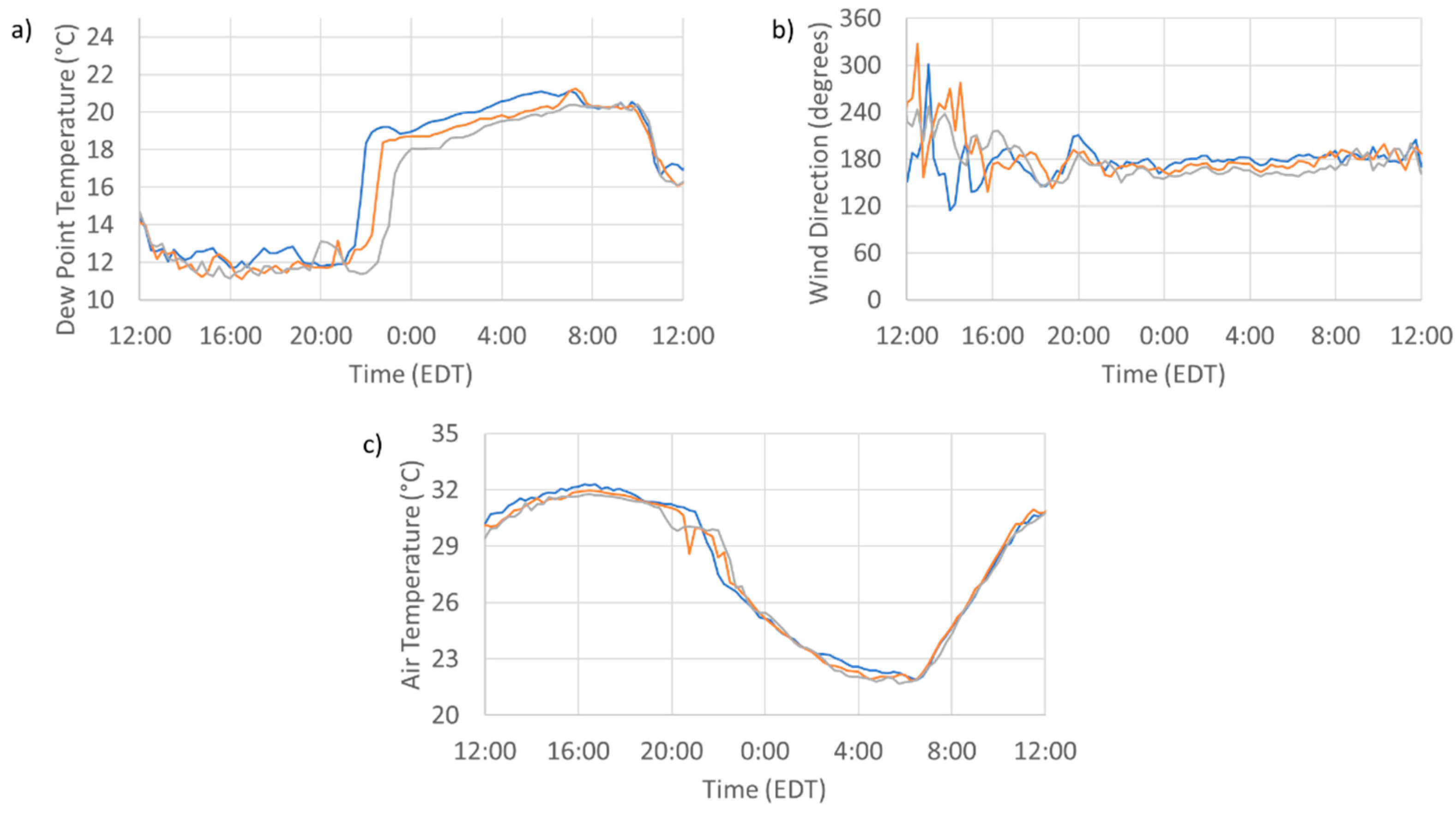
An example of the meteorological conditions during a sea breeze passage is shown in Figure 3 for 22 May 2019. The sea breeze passed over the SRS at approximately 22:00 EDT and can be seen through the modification of atmospheric variables first at MT1, then followed at MT2 and MT3. The dew point temperatures rose six degrees at each tower in succession before continuing to rise throughout the night. The wind direction following the passage of the sea breeze became very consistent with a marked reduction in variation. While this is somewhat consistent with the expected overnight conditions, the fact that the reduction in variance occurred at the same time as the sea breeze passage indicates a contributing influence. The change in the temperature for this case was less pronounced as the temperature is expected to drop overnight. However, at the time of the sea breeze passage, a more noticeable drop of 2–4 °C during a short period of time was observed before resuming a slower rate of decreasing temperature through the night.
To examine the more general behavior of sea breezes, meteorological variables for each day of sea breeze passage were adjusted to be normalized to the time when the sea breeze passed over the region.
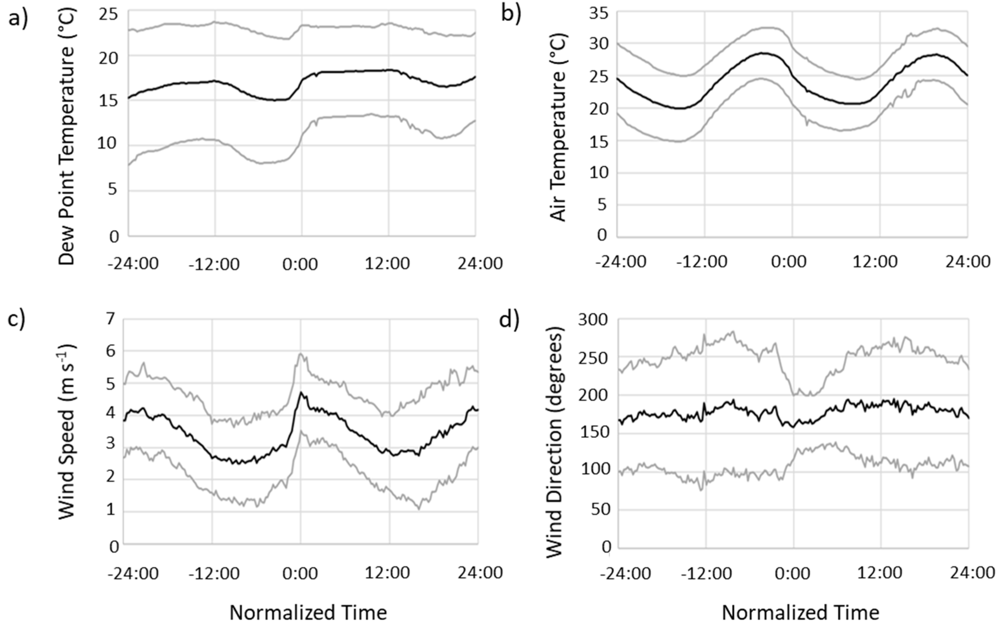
This allows for the changes in meteorological variables at the time of, and following, the sea breeze front passage to be compared. The results are shown in Figure 4 for the average dew point temperature, air temperature, wind direction and wind speed and one standard deviation above and below the average for the 24 h leading up to the sea breeze passage and the 24 h following. The dew point temperature shows a general increase in the hours around the passage of a sea breeze of approximately 3–4 °C, followed by a slow increase during the following night. The dew point temperatures the day following a sea breeze front passing tend to be 2–3 °C higher than the preceding day. The air temperature, however, shows no significant change at the time of the sea breeze frontal passage. Analysis of the raw temperature data suggests that there may be a slightly accelerated cooling effect when the sea breeze passes, but the signal is not robust enough to be separated from the general cooling that is usually occurring when sea breezes arrived at SRS.
Winds also show a distinct pattern of sea breeze passage. While wind speeds tend to follow a pattern that increases during the day and decreases at night, there appears to be a distinct increase in the wind speeds in the hours leading up to the sea breeze that is not apparent on the preceding or following days. The increasing wind speed during the early part, and middle, of the day (generally corresponding to 1500–2200 in Figure 4) is likely the result of the convective turbulence that is acting to mix down higher wind speeds but does not explain the sharp jump at the time of the sea breeze passage that tended to occur after 2000 local time. At that time, convectively driven mixing should have ended, suggesting that the wind speed increase is more likely the result of the sea breeze front arriving. The wind speed then decreased slightly, immediately following the sea breeze passing but then remained steady for a few hours before beginning to decrease through the remainder of the overnight period. While low-level jets do occur over the region, the wind measurement heights are likely to be close enough to the surface that they reside below the height of the jet [18].
Wind direction shows a distinct turning of the winds to the southeast and the south when the sea breeze front passes. While winds on these days tend to be from the south in general, the variation of the winds narrows when the sea breeze passes and remains that way for up to 6 h following the sea breeze front.
An examination of ceilometer backscatter at SRS shows that in many cases, the backscatter increase coincided with when the sea breeze front passed over the site (Figure 5). The change in backscatter indicates changes to the aerosol properties at the surface, which could include larger particles, typical of marine aerosol; swollen particles, deliquesced from higher dewpoints; or a greater particle concentration. Based on the attenuated backscatter profile, it appears the modified near-surface airmass, including aerosols, resulting from the sea breeze would persist overnight until convective mixing began the following day.
3.2. Influence of Synoptic Case on Sea Breeze Frequency
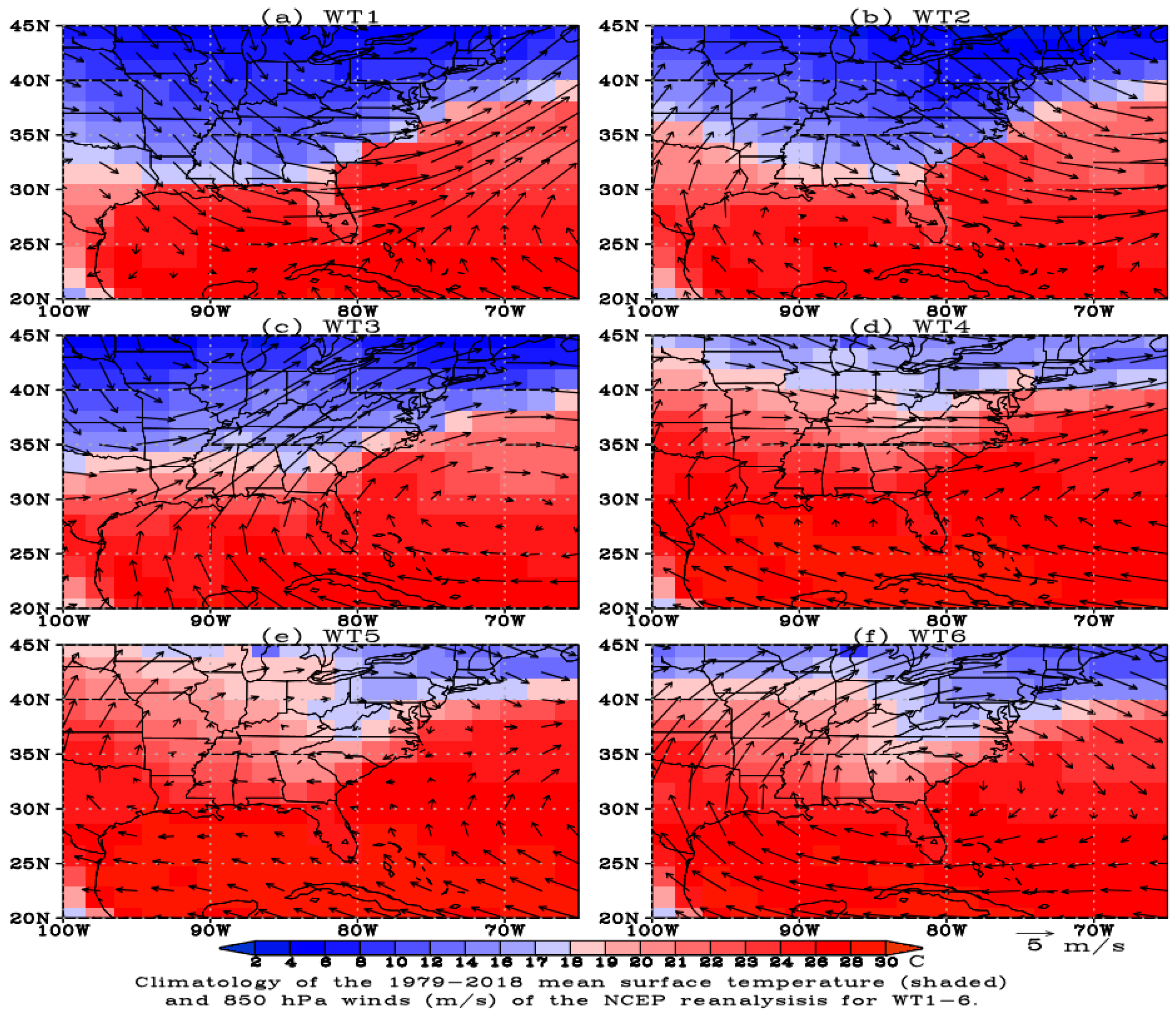
Using K-Means clustering to identify the synoptic wind field classes across the southeastern United States, the maximum CI was found to indicate six classes [19]. The 850 mb wind and surface temperature fields for the classes that were identified are shown in Figure 6. Classes one and two describe the passage of a trough over the eastern United States, leading to strong (class one) and moderate (class two) offshore flow over the SEUS. Class three represents an offshore high-pressure system with moderate flow moving parallel to the coast in the SEUS. Class four represents a fairly zonal flow over the SEUS. Classes five and six represent cases with moderate to broad high-pressure systems over the SEUS with light and variable winds over the region.
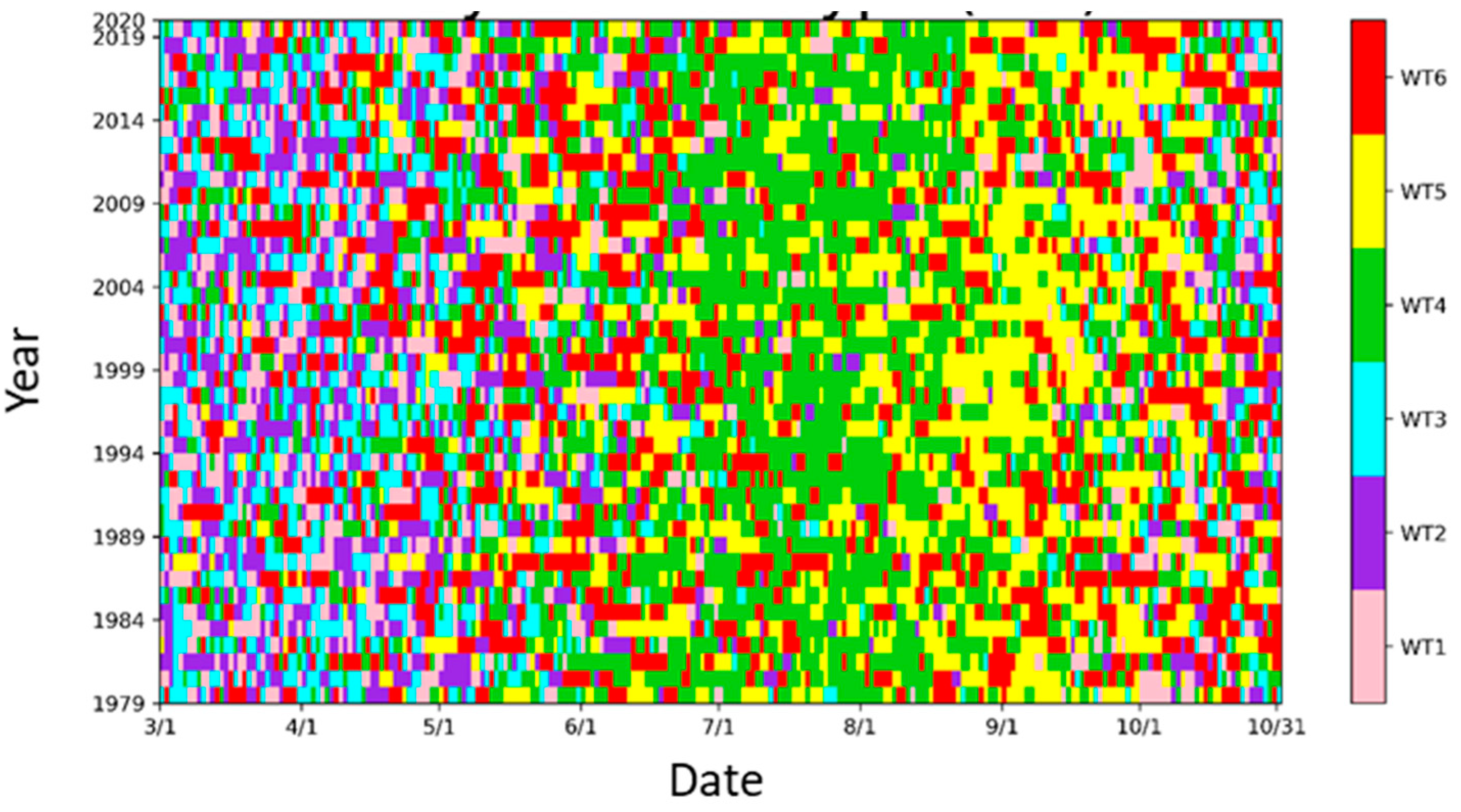
An analysis of the frequency of each classification as a function of the time of year shows a distinct trend in the type of synoptic pattern expected over the SEUS during the course of the spring, summer and early fall [19]. During the months of March and April, there is a mix that consists predominantly of classes one, two, three and six. These cases represent a pattern of high- and low-pressure systems moving over the region during the spring. Beginning in May, classes four, five and six become more prevalent, representing a shift to more high-pressure systems and zonal flow cases with generally lighter wind speeds. From June to August, the prevailing pattern is dominated by class four with generally low-wind cases. Beginning in September, the synoptic flow begins to shift to class five and then slowly returns to a mix of classes one, two, three and six in October.
The number of sea breeze cases identified, classified according to synoptic classification, are shown in Table 2, along with the total number of days (sea breeze and non-sea breeze) that fall under each classification for the March–October period. The majority of sea breeze cases, approximately 63%, occurred under classes four and six. The remaining proportion were spread through classes two, three and five, while only a few inland penetrating sea breezes occurred during class one.
Classes four and six, despite having the majority of sea breeze cases, were not necessarily substantially more prone to sea breeze formation. An analysis of the frequency of sea breeze formation during the occurrence of each synoptic classification shows that 21% of the days with classification two or six had sea breezes, while only 17% of the days in classification four had a sea breeze. This is followed by 13% of the class three days, and less than 10% of the class one and five days. Comparing the precipitation in the six WTs (figure not shown; please refer to [19]) indicated that WT two and six are dry over coastal SEUS. That explains why these two WTs are prone to sea breezes that are mainly driven by the solar radiative heating over coastal land in fair weather.
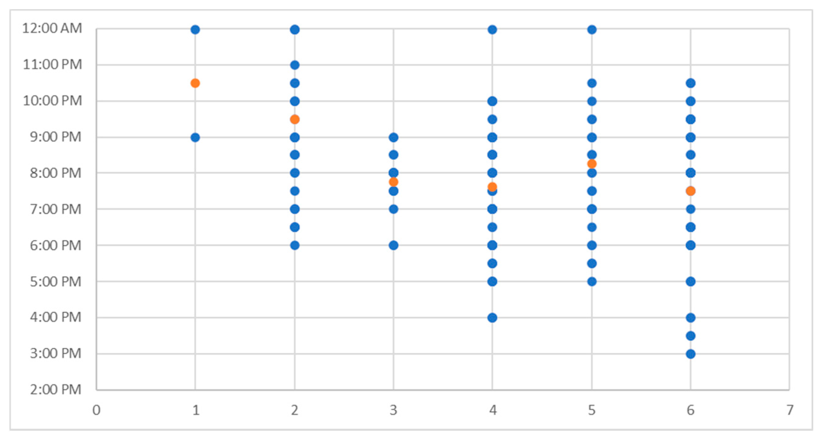
The timing of the sea breeze exhibited a range between arriving between 1500 and 2200 Local Daylight Time (Figure 7). On average, the sea breeze passed over the SRS region at approximately 2000 Local Daylight Time, though for classes one and two, with moderate to strong offshore flow, the arrival of a sea breeze was found to be generally 1–2 h later.
The impact of wind speed on the ability of a sea breeze to move inland is noted in the frequency of sea breezes observed for conditions described by class one and class four. In both these cases, there is southwest synoptic flow in the southeast U.S. and along the coast, but the stronger wind speeds characterized by class one seem to inhibit the ability of sea breezes from moving inland. These findings are consistent with prior studies that, using numerical simulations, reported that sea breezes were suppressed when the flow was directed onshore or when the flow was strongly directed offshore [20,21]. In the case of the flow moving onshore, the signal of the sea breeze would be hidden enmeshed with the broader flow that would have similar characteristics to that of the sea breeze. In the case of a strong offshore flow, the inertia of the sea breeze is unable to overcome the synoptic flow and is confined closer to the coastal region.
Seasonal variations in air and sea surface temperatures clearly play a role in the distribution of sea breezes among the synoptic classes. For instance, the light winds characteristic of class five would seem ideal for sea breeze formation, but a lower proportion of these days exhibited a sea breeze relative to any other class except one. This can be attributed to the fact that class five is more likely to occur in the late summer to early fall, when the sea surface temperature over the Gulf stream area is high; thus, the difference between sea surface temperatures and air temperatures over the land will be reduced, as shown in Figure 8.
We examined the potential for cloud cover to be a contributing factor to the development of a sea breeze as widespread cloud cover would hinder warming during the day. In particular, we hypothesized that an inland sea breeze movement would have some correlation with low cloud fractions. However, no clear signal emerged when comparing days with sea breezes and cloud cover. In fact, there was significant variation with cloud cover on sea breeze days ranging from clear to overcast using cloud data collected at SRS and at ASOS stations located between the South Carolina coast and the SRS.
3.3. Identification of Additional Sea Breezes
The signals observed in the sea breeze air mass are consistent with previously reported analyses of inland moving sea breezes [5]. Given our reliance on using visible signals on radar to identify sea breezes, it is expected that some number of sea breeze fronts were not identified, suggesting that we are underestimating the number of sea breezes that influence inland areas. To examine whether we were missing sea breezes that were not observed passing the SRS on radar, we analyzed the expected conditions in the confirmed cases and then searched for similar cases. The criteria we focused on were indications of an airmass shift based on increased attenuated backscatter profiles from the ceilometer combined with increases in the dew point temperature of 2 °C or greater within an hour, shifts in wind direction to the southeast and reductions in the standard deviation of wind direction at each of the meteorological measurement sites; in particular we looked for these signals to occur in sequential order, beginning with the tower nearest the coast and moving farther inland. This yielded a number of additional days with potential sea breeze, many of which had supporting visual evidence on radar images where a sea breeze was not observed passing over the SRS, but a sea breeze signal was seen nearby and then disappearing from radar. In these cases, based on ceilometer measurements, the sea breeze appeared shallower and, thus, was likely passing under the radar beam by the time it reached the SRS. In some cases where there was no evidence of a sea breeze on radar, it was determined that the cause of the indicative signals was often related to storm activity in the region.
More recently, a Scanning Mobility Particle Sizer (SMPS) was established at the SRS to aid in studying inland sea breeze properties. While the instrument was deployed in 2021, after the period of study, the initial results suggest that the aerosols associated with the sea breeze do tend to be larger than the ambient aerosols observed earlier, preceding the sea breeze arrival (Figure 9). We expect future work to focus on analyzing the difference in aerosol properties and their potential impact on next-day convective boundary layer and cloud formation.
For broader studies to identify the generality of the results of this work, automated methods of identifying sea breezes or those developed through the use of machine learning techniques such as neural networks or random forest models would be worthwhile. For example, one technique was able to identify approximately a third of the sea breezes compared to visual identification [22]. While the goal of AI is to mine through data to identify signals that identify a particular phenomenon, it is helpful to have some idea of what the precursors are that we expect to be identifying. From this work, we would expect wind direction and dew point temperature to be two key parameters that could be used to indicate sea breeze passage.
4. Conclusions
By performing an analysis of sea breeze inland intrusion based on the observations made on radar, we were able to identify some of the underlying conditions that may promote the inland intrusion of sea breeze and the potential effects of the sea breeze. Sea breezes were found to be more prevalent when the synoptic flow was moderately directed offshore (against the direction of sea breeze inland movement) than when the conditions were either strongly opposed to sea breeze movement or when the synoptic flow was moving in the same direction as the sea breeze. For the synoptic cases with a strong offshore flow (class one) and a moderate offshore flow (class two), the average time of the sea breeze arrival was found to be 1 to 2 h later than in any other case.
We have used archived radar imagery in combination with available measurements at the SRS to assess the frequency of sea breezes to move inland. For sea breezes passing over the SRS, this represents a distance of 150–200 km. We have identified that inland advecting sea breezes are a regular occurrence over the region, with approximately 50 sea breezes passing over the SRS each year. These sea breezes result in a modification of the atmosphere that persists overnight and into the morning, most notably including a rise in the dew point temperature and a shift in wind direction to the south or southeast. We have also identified that the aerosol concentration of the atmosphere changes as a result of the sea breeze, leading to higher concentrations of aerosols and generally larger aerosols overnight. Regardless of the specific physics involved in the generation of larger aerosols, whether due to the advection of marine aerosols or a rapid growth of local aerosols as a result of the more humid airmass, these sea breeze intrusions are likely to affect the development of the convective boundary layer and clouds on the following day. Sea breezes were found to occur during all the months from March to October, but with greatest frequency in the spring to early summer, when the landmass is heating up more quickly from solar radiation than the ocean. It was also found that synoptic conditions that consist of moderate offshore flow produced the greatest number of observed inland-moving sea breezes. The sea breeze often modified the atmospheric conditions near the surface to be more humid and developed a southeasterly flow, creating a separate airmass from the synoptic conditions aloft. These conditions would often persist through the night until convective mixing would begin the next morning.
We expect future work to be able to incorporate a spatially distributed dataset of meteorological and satellite observations to identify the frequency and extent of inland moving sea breezes. Accurate characterizations and identification of the underlying signals would be expected to help improve forecasts in a number of areas ranging from cloud predictions to patterns in the rate of nighttime cooling following a sea breeze passage and the daytime warming on the subsequent day. Satellite imagery may depict along-shore coherency in the sea breeze front. Understanding the role of sea breezes has the potential to improve coastal forecasting on scales from regional earth system models to smaller scales of forecasting for solar power and energy consumption. In the SEUS, given the extent of the region that is coastal and the inland areas that are subject to sea breezes, improvements in the forecasting of sea breezes could make substantial improvements to weather forecast accuracy in the region.
Author Contributions
Conceptualization, B.V., S.N., J.-H.Q. and D.W.; methodology, B.V., S.N. and J.-H.Q.; formal analysis, B.V., S.N. and J.-H.Q.; data curation, B.V., S.N. and J.-H.Q.; writing-original draft preparation, B.V.; writing-review and editing, B.V., S.N., J.-H.Q., D.W., P.G., L.P. and S.B.; project administration, S.N.; funding acquisition, S.N. All authors have read and agreed to the published version of the manuscript.
Funding
This work was supported by the Laboratory Directed Research and Development (LDRD) program within the Savannah River National Laboratory (SRNL). This document was prepared in conjunction with work accomplished under Contract No. DE-AC09-08SR22470 with the U.S. Department of Energy (DOE) Office of Environmental Management (EM).
Institutional Review Board Statement
Not applicable.
Informed Consent Statement
Not applicable.
Data Availability Statement
The data presented in this study are available on request from the corresponding author. The data are not publicly available due to database access restrictions.
Acknowledgments
We would like to acknowledge Chuck Hunter who was instrumental in helping establish this research program.
Conflicts of Interest
The authors declare no conflict of interest.
References
- Buckley, R.L.; Kurzeja, R.J. An observational and numerical study of the nocturnal sea breeze. J. Appl. Meteorol. 1997, 36, 531–546. [Google Scholar]
- Miller, S.T.K.; Keim, B.D.; Talbot, R.W.; Mao, H. Sea breeze: Structure, forecasting and impacts. Rev. Geophys. 2003, 41, 1011. [Google Scholar] [CrossRef] [Green Version]
- Simpson, J.E.; Mansfield, D.A.; Milford, J.R. Inland penetration of sea breeze fronts. Q. J. R. Meteorol. Soc. 1977, 103, 47–76. [Google Scholar] [CrossRef]
- Zhou, Y.; Guan, H.; Gharib, S.; Batelaan, O.; Simmons, C.T. Cooling power of sea breezes and its inland penetration in dry-summer Adelaide, Australia. Atmos. Res. 2021, 250, 105409. [Google Scholar] [CrossRef]
- Muppa, S.K.; Anandan, V.K.; Kesarkar, K.A.; Rao, S.V.B.; Reddy, P.N. Study on deep inland penetration of sea breeze over complex terrain in the tropics. Atmos. Res. 2012, 104–105, 209–216. [Google Scholar] [CrossRef]
- Yum, S.S.; Hudson, J.G. Maritime/continental microphysical contrasts in stratus. Tellus B Chem. Phys. Meteorol. 2002, 54, 61–73. [Google Scholar] [CrossRef]
- Dong, X.; Xi, B.; Kennedy, A.; Minnis, P.; Wood, R. A 19-month record of marine aerosol-cloud-radiation properties derived from DOE ARM mobile facility deployment at the Azores. Part I: Cloud fraction and single-layered MBL cloud properties. J. Clim. 2013, 27, 3665–3682. [Google Scholar] [CrossRef] [Green Version]
- Logan, T.; Dong, X.; Xi, B. Aerosol properties and their impacts on surface CCN at the ARM Southern Great Plains Site during the 2011 Midlatitude Continental Convective Clouds Experiment. Adv. Atmos. Sci. 2018, 35, 224–233. [Google Scholar] [CrossRef]
- Lee, S.S.; Donner, L.J.; Phillips, T.J.; Ming, Y. Examination of aerosol effects on precipitation in deep convective clouds during the 1997 ARM summer experiment. Q. J. R. Meteorol. 2008, 134, 1201–1220. [Google Scholar] [CrossRef]
- O’Halloran, T.L.; Fuentes, J.K.; Tao, W.K.; Li, X. Sensitivity of convection to observed variation in aerosol size distributions and composition at a rural site in the southeastern United States. J. Atmos. Chem. 2015, 72, 441–454. [Google Scholar] [CrossRef]
- Chen, G.; Iwai, H.; Ishii, S.; Saito, K.; Seko, H.; Sha, W.; Iwasaki, T. Structures of the sea breeze front in dual-doppler lidar observation and coupled mesoscale-to-LES modeling. J. Geophys. Res. Atmos. 2019, 124, 2397–2413. [Google Scholar] [CrossRef]
- Weinbeck, S.; Viner, B.; Rivera-Giboyeaux, A. Meteorological monitoring program at the Savannah River Site. In SRNL-TR-2020-00197 Rev. 0; Savannah River National Laboratory: Aiken, SC, USA, 2020. [Google Scholar]
- Moron, V.; Robertson, A.W.; Ward, M.N.; Ndiaye, O. Weather types and rainfall over Senegal. J. Clim. 2008, 21, 266–287. [Google Scholar] [CrossRef] [Green Version]
- Qian, J.-H.; Robertson, A.W.; Moron, V. Interaction among ENSO, the monsoon and diurnal cycle in rainfall variability over Java, Indonesia. J. Atmos. Sci. 2010, 67, 3509–3524. [Google Scholar] [CrossRef]
- Qian, J.-H.; Robertson, A.W.; Moron, V. Diurnal cycle in different weather regimes and rainfall variability over Borneo associated with ENSO. J. Clim. 2013, 26, 1772–1790. [Google Scholar] [CrossRef]
- Qian, J.-H. Multi-scale climate processes and rainfall variability in Sumatra, Peninsula Malaysia and Singapore associated with ENSO in boreal fall and winter. Int. J. Clim. 2020, 40, 4171–4188. [Google Scholar] [CrossRef]
- Roller, C.D.; Qian, J.-H.; Agel, L.; Barlow, M.; Moron, V. Winter weather regimes in the Northeast United States. J. Clim. 2016, 29, 2963–2980. [Google Scholar] [CrossRef]
- Werth, D.; Buckley, R.; Zhang, G.; Kurzeja, R.; Leclerc, M.; Duarte, H.; Parker, M.; Watson, T. Quantifying the local influence at a tall tower site in nocturnal conditions. Theor. Appl. Clim. 2017, 127, 627–642. [Google Scholar] [CrossRef]
- Qian, J.-H.; Viner, B.; Noble, S.; Werth, D. Precipitation characteristics of warm season weather types in the southeastern United States of America. Mon. Wea. Rev. 2021. In Review. [Google Scholar]
- Arritt, R.W. Effects of the large-scale flow on characteristic features of the sea breeze. J. Appl. Meteorol. 1993, 32, 116–125. [Google Scholar] [CrossRef] [Green Version]
- Chen, F.; Miao, S.; Tewari, M.; Bao, J.-W.; Kusaka, H. A numerical study of interactions between surface forcing and sea breeze circulations and their effects on stagnation in the greater Houston area. J. Geophys. Res. 2011, 116, D12105. [Google Scholar] [CrossRef] [Green Version]
- Azorin-Molina, C.; Tijm, S.; Chen, D. Development of selection algorithms and databases for sea breeze studies. Theor. Appl. Clim. 2011, 106, 531–567. [Google Scholar] [CrossRef]
Figure 1.
A depiction of the sea breeze signal as observed on radar from 13–14 May 2018.

Figure 2.
Map of the geographical region between the South Carolina coast and the SRS. The inset in the upper-right shows the locations of MT1, MT2 and MT3 on the SRS.
Figure 2.
Map of the geographical region between the South Carolina coast and the SRS. The inset in the upper-right shows the locations of MT1, MT2 and MT3 on the SRS.

Figure 3.
Depiction of 61 m (a) dew point temperature, (b) wind direction and (c) temperature on 22 May 2019 at MT1 (blue), MT2 (orange) and MT3 (gray).
Figure 3.
Depiction of 61 m (a) dew point temperature, (b) wind direction and (c) temperature on 22 May 2019 at MT1 (blue), MT2 (orange) and MT3 (gray).

Figure 4.
Average (thick) and one standard deviation above and below for (a) dew point temperature, (b) temperature, (c) wind speed and (d) wind direction for sea breeze cases at MT1, including the 24 h prior to and after the time of sea breeze passage at MT1. Times have been normalized to ensure that the time of the sea breeze passage is adjusted to be 0:00 in the center of the plots.

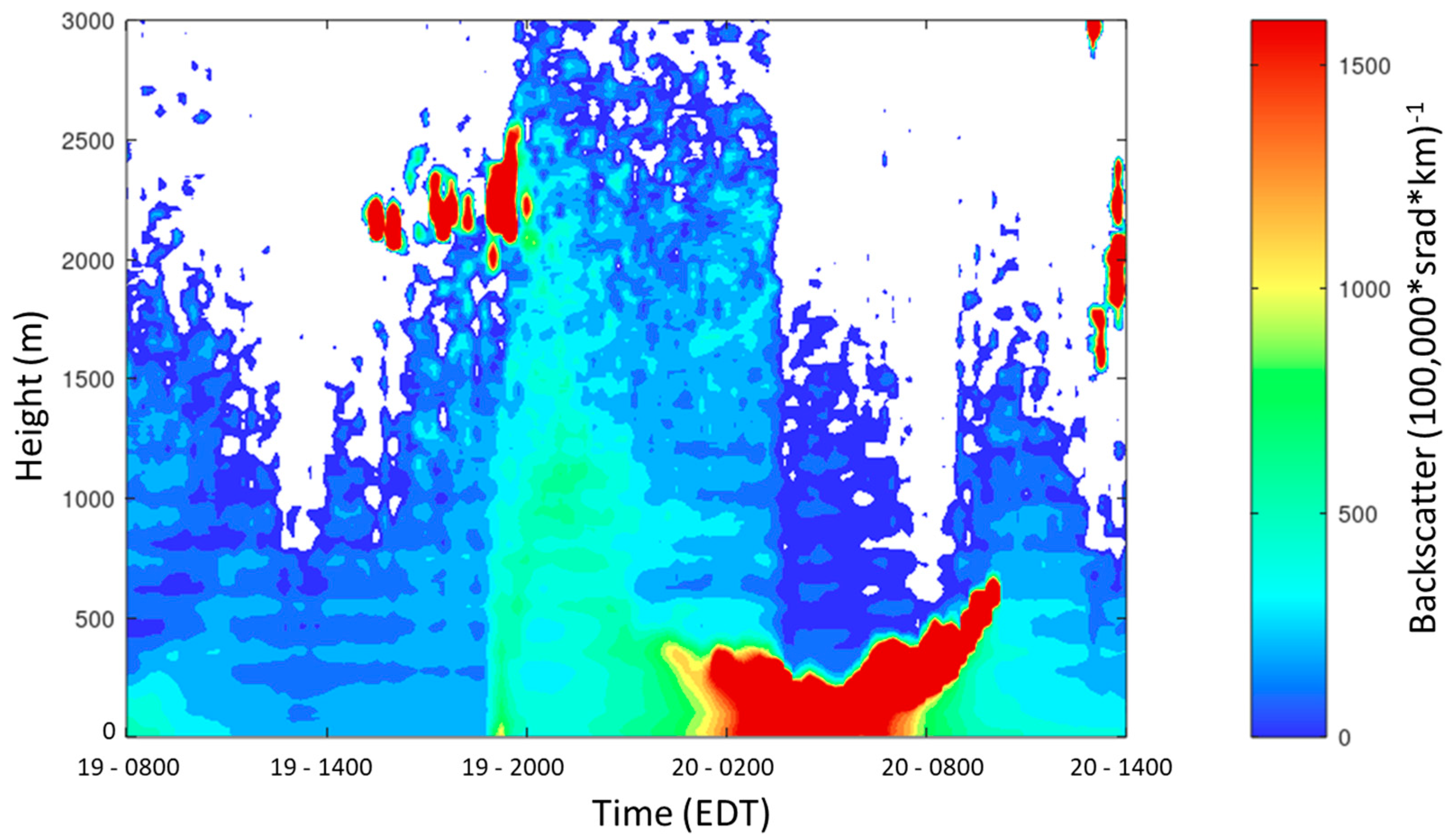
Figure 5.
Backscatter from the SRS ceilometer for 2019 May 19 and 20. A sea breeze front passes at 1900 EDT on May 19.
Figure 5.
Backscatter from the SRS ceilometer for 2019 May 19 and 20. A sea breeze front passes at 1900 EDT on May 19.

Figure 6.
Description of the 850 mb wind fields for each of the six synoptic-scale classifications identified using K-means clustering analysis.
Figure 6.
Description of the 850 mb wind fields for each of the six synoptic-scale classifications identified using K-means clustering analysis.

Figure 7.
Depiction of the occurrence of different synoptic classification over the SEUS as a function of time of year for the March–October study period between 1979 and 2020.
Figure 7.
Depiction of the occurrence of different synoptic classification over the SEUS as a function of time of year for the March–October study period between 1979 and 2020.

Figure 8.
Summary of estimated times when the sea breeze was observed to arrive at the SRS based on 30-min visual observation of radar imagery and grouped by synoptic case (blue) and the average time that the sea breeze arrived for each synoptic case (orange).
Figure 8.
Summary of estimated times when the sea breeze was observed to arrive at the SRS based on 30-min visual observation of radar imagery and grouped by synoptic case (blue) and the average time that the sea breeze arrived for each synoptic case (orange).

Figure 9.
Particle size and concentrations for a sea breeze on 10 March 2021 using an SMPS. The sea breeze passed at approximately 0030 UTC, which coincides with a rapid increase in particle concentrations in the 50–200 nm range. Times in the top plot are relative to the approximate time the sea breeze arrived at the SMPS.


Table 1.
Frequency of sea breeze occurrence as observed using radar categorized by month and year. The two months in each year with the highest frequency are italicized; 2016 has three months italicized because March and April each had 6 observed sea breezes.
Table 1.
Frequency of sea breeze occurrence as observed using radar categorized by month and year. The two months in each year with the highest frequency are italicized; 2016 has three months italicized because March and April each had 6 observed sea breezes.
| Year | Month | |||||||
|---|---|---|---|---|---|---|---|---|
| Mar | Apr | May | Jun | Jul | Aug | Sep | Oct | |
| 2015 | 2 | 3 | 9 | 5 | 6 | 3 | 0 | 0 |
| 2016 | 6 | 6 | 4 | 9 | 3 | 2 | 0 | 0 |
| 2017 | 6 | 14 | 6 | 7 | 3 | 5 | 1 | 1 |
| 2018 | 2 | 8 | 11 | 6 | 6 | 6 | 6 | 2 |
| 2019 | 3 | 5 | 7 | 1 | 2 | 7 | 4 | 0 |
Table 2.
Number of days between March and October, categorized by year and synoptic case, for (top) sea breeze cases only, (middle) all days and (bottom) the fraction of days experiencing a sea breeze.
Table 2.
Number of days between March and October, categorized by year and synoptic case, for (top) sea breeze cases only, (middle) all days and (bottom) the fraction of days experiencing a sea breeze.
| Year | Class | ||||||
| 1 | 2 | 3 | 4 | 5 | 6 | Total | |
| 2015 | 0 | 4 | 2 | 8 | 5 | 9 | 28 |
| 2016 | 0 | 7 | 4 | 8 | 2 | 9 | 30 |
| 2017 | 1 | 5 | 5 | 17 | 3 | 12 | 43 |
| 2018 | 1 | 3 | 5 | 16 | 8 | 14 | 47 |
| 2019 | 0 | 8 | 1 | 10 | 1 | 9 | 29 |
| 2015–2019 | 2 | 27 | 17 | 59 | 19 | 53 | |
| Year | Class | ||||||
| 1 | 2 | 3 | 4 | 5 | 6 | Total | |
| 2015 | 15 | 25 | 18 | 73 | 61 | 53 | 245 |
| 2016 | 24 | 24 | 30 | 61 | 47 | 59 | 245 |
| 2017 | 24 | 21 | 33 | 84 | 41 | 42 | 245 |
| 2018 | 29 | 31 | 19 | 75 | 43 | 48 | 245 |
| 2019 | 20 | 28 | 30 | 64 | 47 | 56 | 245 |
| 2015–2019 | 112 | 129 | 130 | 357 | 239 | 258 | |
| Year | Class | ||||||
| 1 | 2 | 3 | 4 | 5 | 6 | ||
| 2015 | 0 | 0.16 | 0.11 | 0.11 | 0.08 | 0.17 | |
| 2016 | 0 | 0.29 | 0.13 | 0.13 | 0.04 | 0.15 | |
| 2017 | 0.04 | 0.24 | 0.15 | 0.2 | 0.07 | 0.29 | |
| 2018 | 0.03 | 0.1 | 0.26 | 0.21 | 0.19 | 0.29 | |
| 2019 | 0 | 0.29 | 0.03 | 0.16 | 0.02 | 0.16 | |
| 2015–2019 | 0.02 | 0.21 | 0.13 | 0.17 | 0.08 | 0.21 | |
Publisher’s Note: MDPI stays neutral with regard to jurisdictional claims in published maps and institutional affiliations. |
© 2021 by the authors. Licensee MDPI, Basel, Switzerland. This article is an open access article distributed under the terms and conditions of the Creative Commons Attribution (CC BY) license (https://creativecommons.org/licenses/by/4.0/).
Share and Cite
MDPI and ACS Style
Viner, B.; Noble, S.; Qian, J.-H.; Werth, D.; Gayes, P.; Pietrafesa, L.; Bao, S. Frequency and Characteristics of Inland Advecting Sea Breezes in the Southeast United States. Atmosphere 2021, 12, 950. https://doi.org/10.3390/atmos12080950
AMA Style
Viner B, Noble S, Qian J-H, Werth D, Gayes P, Pietrafesa L, Bao S. Frequency and Characteristics of Inland Advecting Sea Breezes in the Southeast United States. Atmosphere. 2021; 12(8):950. https://doi.org/10.3390/atmos12080950
Chicago/Turabian StyleViner, Brian, Stephen Noble, Jian-Hua Qian, David Werth, Paul Gayes, Len Pietrafesa, and Shaowu Bao. 2021. "Frequency and Characteristics of Inland Advecting Sea Breezes in the Southeast United States" Atmosphere 12, no. 8: 950. https://doi.org/10.3390/atmos12080950
Note that from the first issue of 2016, this journal uses article numbers instead of page numbers. See further details here.