
Bayesian and E-Bayesian Estimations of Bathtub-Shaped Distribution under Generalized Type-I Hybrid Censoring


Department of Mathematics, Beijing Jiaotong University, Beijing 100044, China
*
Author to whom correspondence should be addressed.
Entropy 2021, 23(8), 934; https://doi.org/10.3390/e23080934
Submission received: 5 June 2021
/
Revised: 8 July 2021
/
Accepted: 17 July 2021
/
Published: 22 July 2021
Abstract
:For the purpose of improving the statistical efficiency of estimators in life-testing experiments, generalized Type-I hybrid censoring has lately been implemented by guaranteeing that experiments only terminate after a certain number of failures appear. With the wide applications of bathtub-shaped distribution in engineering areas and the recently introduced generalized Type-I hybrid censoring scheme, considering that there is no work coalescing this certain type of censoring model with a bathtub-shaped distribution, we consider the parameter inference under generalized Type-I hybrid censoring. First, estimations of the unknown scale parameter and the reliability function are obtained under the Bayesian method based on LINEX and squared error loss functions with a conjugate gamma prior. The comparison of estimations under the E-Bayesian method for different prior distributions and loss functions is analyzed. Additionally, Bayesian and E-Bayesian estimations with two unknown parameters are introduced. Furthermore, to verify the robustness of the estimations above, the Monte Carlo method is introduced for the simulation study. Finally, the application of the discussed inference in practice is illustrated by analyzing a real data set.
1. Introduction
1.1. Bathtub-Shaped Distribution
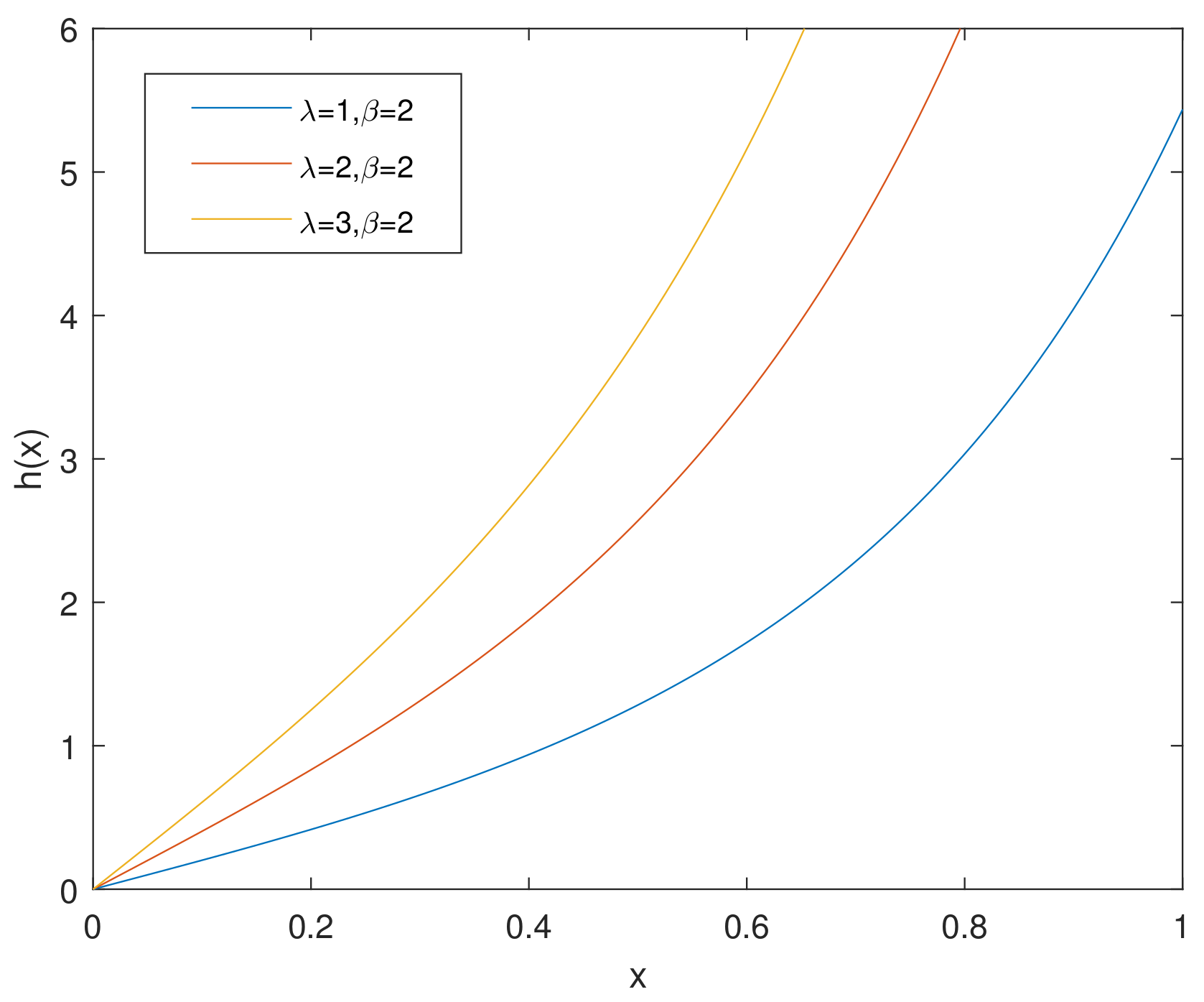
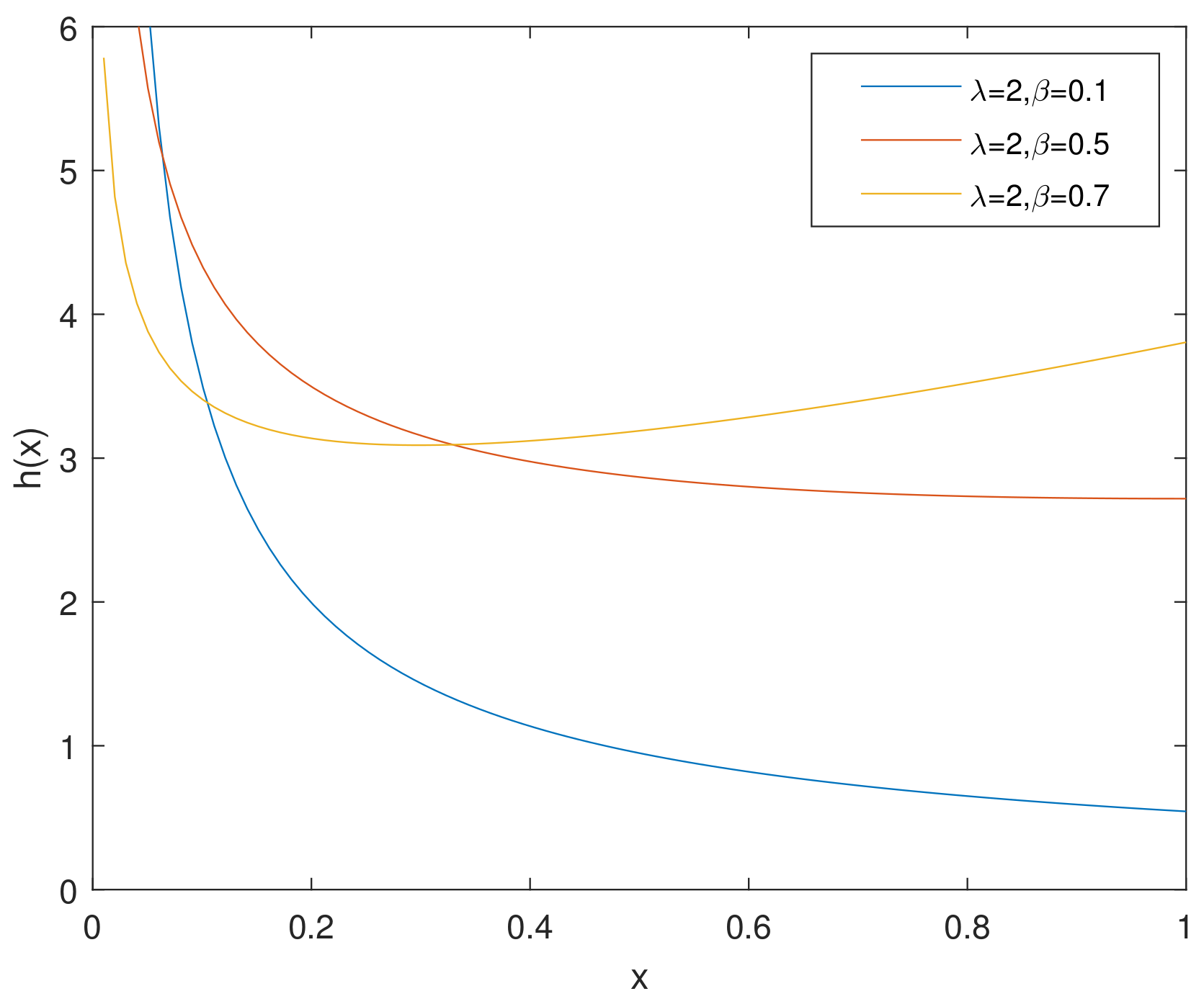
Chen [1] used the term ‘bathtub-shaped distribution’ to refer to a lifetime distribution that possesses an increasing or bathtub-shaped hazard function with two parameters. As it could depict the lifetimes for multiple mechanical and electrical products, this distribution is widely used in practice. There have been several further investigations into the study of bathtub-shaped distribution. Before [1] named the two-parameter lifetime distribution with the above characteristics of a hazard rate function as a bathtub-shaped distribution, a reliability distribution with a bathtub-shaped failure rate was proposed by [2], and ref. [3] employed an effective method to analyze data with a bathtub failure rate by introducing the exponentiated Weibull family.
Furthermore, ref. [4] considered the Bayes estimations and estimates of two unknown parameters based on the maximum likelihood method under a bathtub-shaped distribution. Additionally, a considerable amount of literature has been published on estimations under bathtub-shaped distribution based on a censoring scheme. The authors in [5] focused on the maximum likelihood method to calculate point estimators and derived an exact joint confidence region and confidence interval of parameters based on a progressively Type-II censoring sample. The researchers in [6] investigated the Fisher information matrix, maximum likelihood estimates, and confidence intervals for unknown parameters under hybrid censored data.
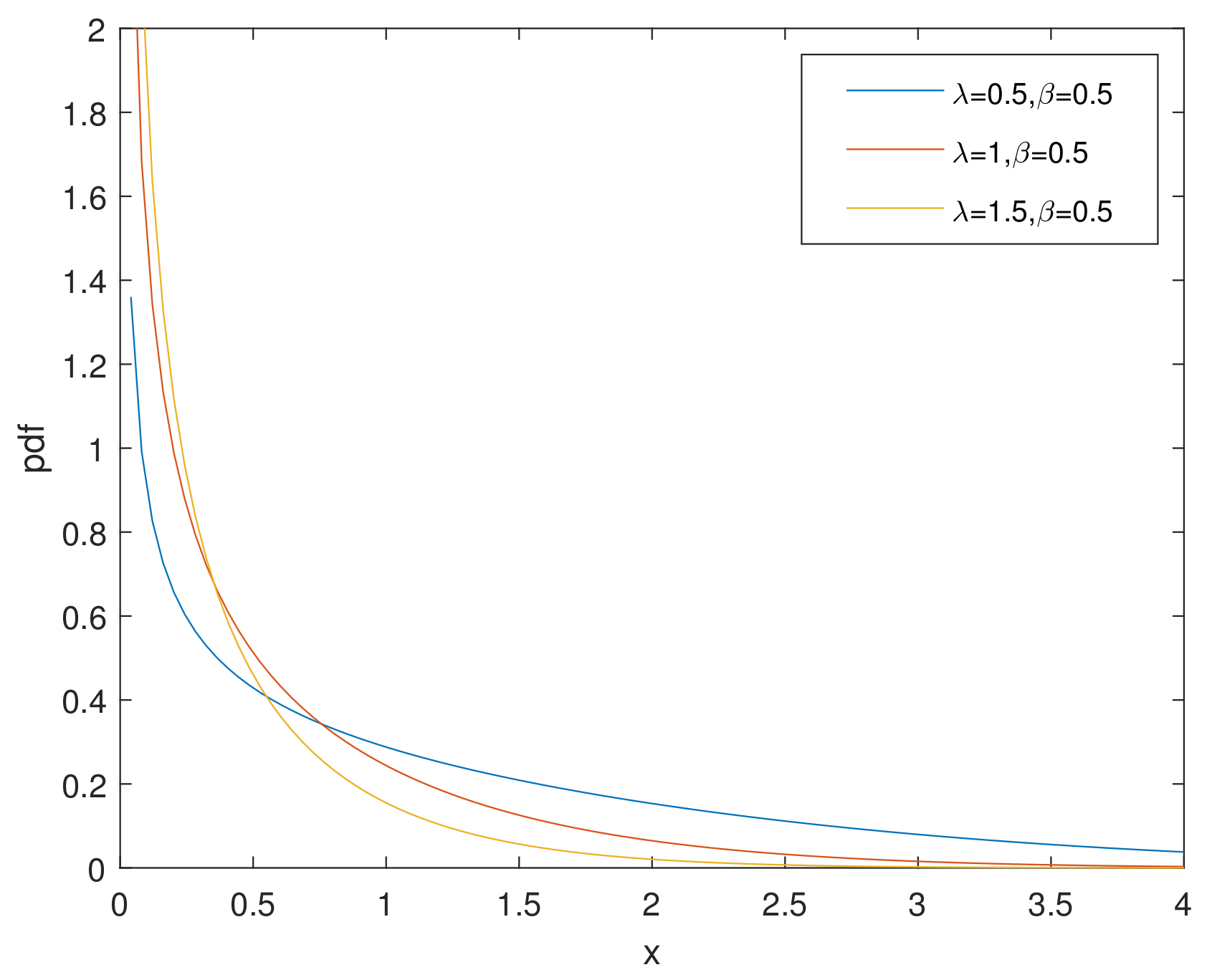
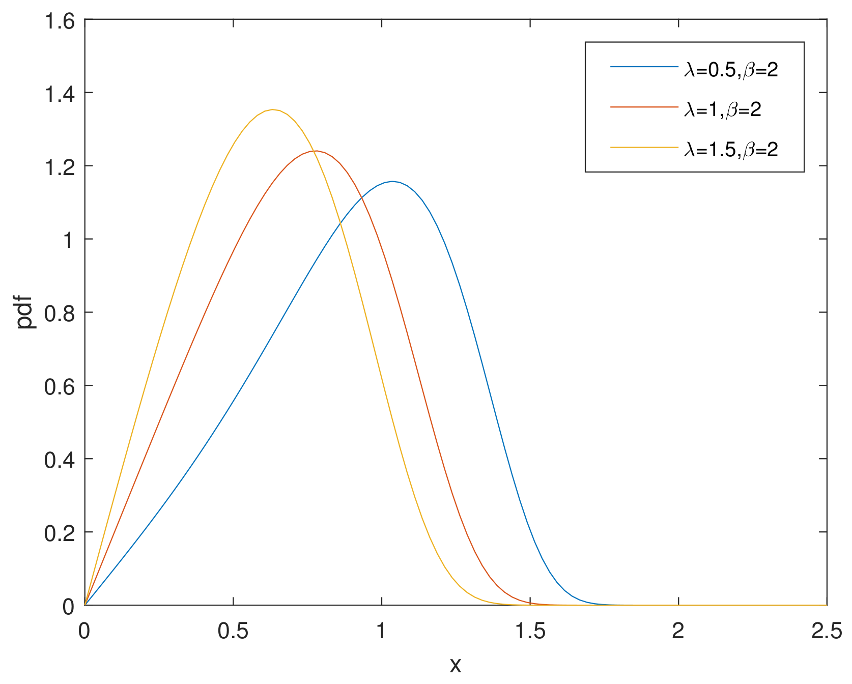
The probability density function (pdf) and cumulative distribution function of a bathtub-shaped distribution take the forms, respectively,
The reliability function and hazard rate function are given by
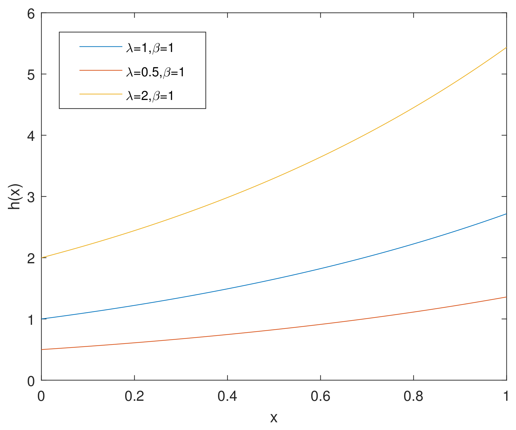
For simplicity, we denote the bathtub-shaped distribution as with the parameters . The parameter has few influence on the shape of its hazard rate function; however, makes a difference to the hazard rate function instead. is bathtub-shaped if the shape parameter , otherwise it appears as an increasing function. In particular, according to [7], when , reduces to the exponential power distribution. Figure 1 and Figure 2 and Figure 3, Figure 4 and Figure 5 show the pdf and of a bathtub-shaped distribution, respectively.
1.2. Generalized Hybrid Type-I Censoring Scheme
There is no doubt that estimations based on complete samples are more accurate. However, it is inevitable to use censoring for lifetime experiments due to time constraints and expense reduction. Type-I and Type-II censoring are usually considered as two fundamental methods to conduct lifetime experiments, where we terminate these experiments at a certain time point or upon the occurrence of a certain number of failures. With the rapid development of science and technology, products have higher reliability and longer life spans, resulting in a longer time of life-testing to obtain sufficient failure samples.
In order to cut down the life-testing duration, ref. [8] carried out a hybrid Type-I censoring scheme that could be considered as a combination of those two fundamental censoring schemes discussed above. Under this scheme, lifetime experiments operate after a specific point of time and the number of failures is pre-fixed. As long as either of these occurs, the test will be terminated. However, this scheme also has limitations as it has a possibility that extremely few failures occur before the pre-determined time. As a result, it may be impractical to make statistical inferences under such a scheme.
In order to overcome this disadvantage and improve the efficiency of estimators in the life-testing experiment as well as to guarantee that a certain number of failures appear before the end of the experiment as well as saving the time of testing and the cost resulted from failures of units, ref. [9] introduced a generalized hybrid Type-I censoring scheme. Generalized hybrid Type-I censoring assures a minimum number of failures, which could mitigate the short back that exists in hybrid Type-I censoring. For simplicity, we denote this as Type-I GHCS.
We assume that , are n ordered observations of failure lifetime. r and T are fixed in advance, where r represents the ideal number of failures and T is the timepoint. These three mentioned censoring models can be expressed as
- Type-I censoring: terminate at T.
- Hybrid Type-I censoring: terminate at .
- Type-I GHCS: terminate at where and k is the minimum acceptable number of failures fixed before the experiment.
In this article, we focus on Type-I GHCS, and it can be divided into three cases:
- Case I: , when .
- Case II: , when .
- Case III: , when .
Ref. [9] introduced exact likelihood estimation of exponential lifetime distribution based on GHCS. Ref. [10] discussed inferential issues under hybrid censoring schemes and presented details on developments regarding generalized hybrid censoring. Ref. [11] studied estimations of a single parameter from a Burr-X distribution under Type-I GHCS. Furthermore, ref. [12] applied an acceptance sampling plan under Weibull distribution under GHCS.
Suppose that is the i-th failure time based on samples from a bathtub-shaped distrubtion under Type-I GHCS. The likelihood function is shown as
where , , , , and D represents the number of failures before timepoint T.
The MLE of parameter can be derived by the equation below,
.
From the equation above, the MLE of is obtained as
By the same method, the MLE of parameter can be derived by the equation,
Previous studies based on bathtub-shaped distribution have always dealt with censored samples under a typical statistical inference method—maximum likelihood estimation for instance. Ref. [13] investigated the estimation problems of unknown parameters, reliability, hazard rate functions, and their approximate confidence intervals under the maximum likelihood method and credible intervals under the Bayesian estimation method.
However, there has been no previous study to coalesce a generalized Type-I hybrid censoring scheme with a bathtub-shaped distribution under the E-Bayesian method. Therefore, our main purpose is to investigate estimations of the scale parameters and reliability function of bathtub-shaped distribution under E-Bayesian and Bayesian methods based on a generalized Type-I hybrid censoring scheme with the presupposition that the shape parameter is known.
The remainder of this paper is organized as follows. Section 2 investigates Bayesian estimations against squared error and LINEX loss functions under Type-I GHCS. Section 3 compares the E-Bayesian estimations derived from three different prior distributions. Section 4 introduces Bayesian and E-Bayesian estimations with two unknown parameters. Section 5 establishes the results of a Monte Carlo simulation study with the Metropolis–Hasting algorithm for the purpose of evaluating the effects of different methods and prior distributions on estimators. Section 5 presents a numerical example from a real data set for the purpose of examining the theoretical inference discussed above.
2. Bayesian Estimation
Bayesian estimation measures the uncertainties of unknown parameters by connecting the prior information from a random sample with certain distributions. Prior distributions as well as loss functions affect the accuracy of estimation under the Bayesian method. In this section, under two different loss functions, we assume the parameter is known and calculate the estimation of scale parameter and the reliability function under a bathtub-shaped distribution based on Type-I GHCS. Then, we derive Bayesian estimations.
First, we suppose that follows the gamma conjugate prior distribution given by:
On the basis of the Bayesian method, we multiply (10) by (5) to obtain the posterior distribution of
where and could be written in the following form
First, we adopt a symmetrical loss function called the squared error (SE) loss function, which lays weight equally on overestimation and underestimation. Based on this loss function, Bayesian estimations are equivalent to the posterior means, which could be obtained to be, respectively,
where .
Secondly, we consider a LINEX loss function with an asymmetric shape, which is commonly used in practice as it is more realistic to illustrate the loss according to ratio. The Bayesian estimation of against the LINEX loss function can be given by
Similarly, the Bayesian estimator of , under a LINEX loss function, is derived in the following form:
3. E-Bayesian Estimation
Considering that the prior information may be deficient, the E-Bayesian method could be used to settle the uncertainty by introducing a class of priors. The authors in [14] demonstrated that, based on a specified prior distribution, the purpose of the E-Bayesian method is to estimate unknown parameters or to predict values of a sequence of random variables.
Under SE and LINEX loss functions, we derive E-Bayesian estimators of and the reliability function. Additionally, for the purpose of perceiving the effects of prior distributions on E-Bayesian estimations, three different prior distributions are considered. The authors in [15] indicated that, in order to ensure that is decreasing, the hyper parameters a and b are chosen. In the case of , the derivative of could be obtained as
It is apparent that the prior distribution is a decreasing function in when and . Assume that the bivariate density function in which a and b are independent is
According to [16], when the parameter a is given, with the increase of b, the tailed prior distribution will be thinner, which would likely reduce the robustness of Bayesian estimations. Therefore, b is selected to be smaller than a pre-determined constant c. In this case, for parameter and , the E-Bayesian estimations are obtained as
Next, for the purpose of exploring the influence of a prior distribution on an estimator under the E-Bayesian method, we derive the estimates under three different prior distributions. These three different prior distributions are selected as follows:
where is the beta function. is a constant in b, while is a decreasing function in b and is an increasing function in b.
3.1. E-Bayesian Estimations Based on SE Loss Function
Based on the SE loss function, the E-Bayesian estimations of with the prior distribution can be obtained from (13), (17) and (19) as
where , , .
Likewise, the E-Bayesian estimations of under and could be written, respectively, in the following forms:
3.2. E-Bayesian Estimations Based on a LINEX Loss Function
Under a LINEX loss function, the E-Bayesian estimation of with the prior distribution can be obtained from (14), (17), and (19) as
Under the same method, the E-Bayesian estimations of under and could be written, respectively, as
3.3. E-Bayesian Estimations of
The E-Bayesian estimation of under an SE loss function can be derived from (15), (17) and (19) by using the prior distribution ,
where is the generalized hypergeometic function. For more details, one can refer to [17].
Under and , the E-Bayesian estimations of are written in the following forms under the same method.
4. Estimation with Two Unknown Parameters
4.1. Bayesian Estimation
In this section, we assume that and are independent and follow a gamma prior distribution:
Thus, the joint prior distribution is obtained as
On the basis of Bayesian method, we multiply (32) by (5) to obtain the joint posterior distribution
where and could be written in the following form
Similarly, we could obtain the Bayesian estimations of two unknown parameters and under SE and LINEX loss functions.
We could not directly calculate these above integrals in simple closed form, but the approximate Bayesian estimators could be derived under Lindley’s aprroximation. For more details, one can refer to [18].
4.2. E-Bayesian Estimation
According to E-Bayesian estimation with unknown parameter , we select the prior distributions for parameter and as follows,
where and are beta functions. Under an SE loss function, the E-Bayesian estimations can be obtained from (40), (41), (35), and (37) as,
Under a LINEX loss function, the E-Bayesian estimations can be obtained from (40), (41), (36), and (38) as,
Similarly, we could use the MCMC method to compute E-Bayesian estimations.
5. MCMC Method and Simulation Study
According to the Markov Chain Monte Carlo algorithm, we could approximate the integral when it cannot be generated explicitly for multidimensional problems. Therefore, the MCMC algorithm is a widely used and effective method to obtain samples from complex posterior distributions. We apply the Monte Carlo simulation under Type-I GHCS in this section to compute E-Bayesian estimates of and against different prior distributions and loss functions.
According to (11), the full conditional posterior probability density function of the parameter is written as,
As the conditional posterior PDF of is complex, we introduce the MCMC method to obtain random samples by considering a normal distribution as the proposal distribution.
The MCMC approach is shown in Algorithm 1. We could refer to [19,20] for more details regarding the implementation of MCMC algorithm.
| Algorithm 1 MCMC algorithm. |
|
For Bayesian and E-Bayesian methods, for the purpose of evaluating and comparing the performance of estimators against different loss functions, we perform simulation comparisons with data derived from different scenarios. We assume that parameter is fixed as constant 1. Given a particular value to c, a and b can be obtained according to (19). The algorithm of generating and analyzing data based on Type-I GHCS under the bathtub-shaped distribution is shown in Algorithm 2.
| Algorithm 2 The algorithm of generating and analyzing data. |
|
Under different , we draw samples from every simulation, and values of are computed. Additionally, we obtain the and Bayesian estimation under each simulation.
In order to facilitate the simulation, according to [21], we take the special case
where .
In this case, the of could be obtained as,
The sample size is fixed from the data under Type-I GHCS and is set to with three sets of fixed numbers presented respectively for each size. Simultaneously, for the purpose of studying the reliability function under a bathtub-shaped distribution, we set T as .
Based on the tabulated estimates and the mean square errors of the estimations whose statistical inference processes are computed from software R, the following conclusion can be drawn from Table 1, Table 2, Table 3, Table 4, Table 5 and Table 6 and Table 7, Table 8 and Table 9, in which the true value of takes 4.37 and 2.5, respectively, and represents the mean square error of the E-Bayesian estimations. Table 1, Table 2, Table 3 and Table 4 show the results of estimations when in detail. Table 5, Table 6, Table 7, Table 8 and Table 9 guarantee the robustness of the conclusion. See more details on the MCMC outputs in Appendix A.
- 1.
- Both estimates are close to their theoretical values under different methods and loss functions.
- 2.
- The mean square errors of the E-Bayesian estimations of parameter and are smaller than those of the Bayesian estimations. Therefore, the efficiency of the E-Bayesian method is higher in the sense of a smaller .
- 3.
- The of estimations under an SE loss function are less than those based on a LINEX loss function. Thus, the SE loss function is more efficient to generate estimates.
- 4.
- As increases, the of the estimate decreases, and the average interval length of reduces. To conclude, the performance of estimates will improve with the size of the sample increases.
6. Illustrative Example
In order to clarify the algorithms and examine the accuracy and robustness of the theoretical results discussed above, we analyze a real data set of the number of cycles to failure from the electrical devices given by [22]. The authors in [4] divided each data point by 1000 in order to compute effectively, and they tested and concluded that the hazard rate of this data set was bathtub-shaped. Table 10 illustrates the electrical lifetime data in detail in which the unit of the data is the number of cycles.
When analyzing this data set under Type-I GHCS, we assume that and evaluate estimates against SE and LINEX loss functions.
Under this assumption, .
Thus, the terminated time will be , and the number of failures is 18. According to (8), the MLE of parameter is obtained as: .
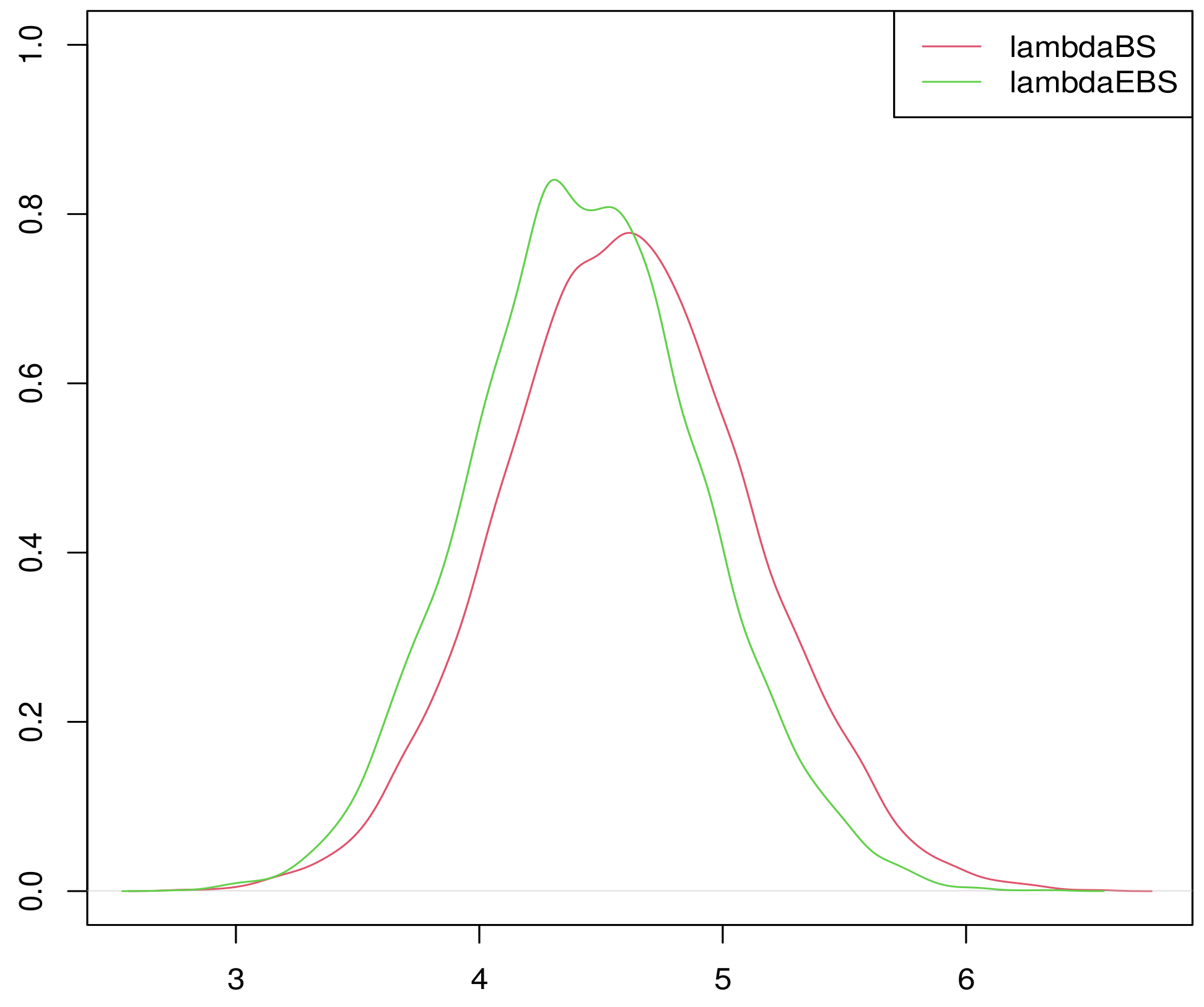
According to Table 11 and Table 12, the good performance of Bayesian and E-Bayesian estimations against different loss functions can be certified. The estimates are consistent with the real data sets. Similarly, we can determine that the of parameter and based on the E-Bayesian approach are smaller than those under the Bayesian approach. It is also more efficient to evaluate estimates against the SE loss function. These are consistent with the statistical inference and numerical simulation results. Thus, it is reasonable to conclude that the theoretical results discussed above are accurate and robust.
7. Conclusions
The bathtub-shaped distribution is crucial in mechanical and electronic research. In addition, it is more efficient to estimate parameters under Type-I GHCS for product testing situations in practice, as this could save the time of testing and the cost resulting from failures of units.
In this article, in order to make estimations under a bathtub-shaped distribution, the Bayesian and E-Bayesian methods were introduced. According to Bayesian theory, we could generate statistical inference from the prior information. With the assumption that the prior distribution follows a gamma distribution, we could derive the estimates of parameter and reliability functions under different loss functions.
We presented the MCMC method in simulation and with a real lifetime example of electronic data to illustrate the statistical inferences discussed above. Under different sample sizes, parameter values and loss functions, we observed that the E-Bayesian method and SE loss function were more efficient in terms of the mean square error. Our study is useful and efficient for experimenters to examine the quality of industrial products. Additionally, this research can be further developed to address practical problems based on multiple censoring schemes.
Author Contributions
Investigation, Y.Z.; Investigation, K.L.; Supervision, W.G. All authors have read and agreed to the published version of the manuscript.
Funding
This research received no external funding.
Data Availability Statement
The data presented in this study are openly available in [22].
Conflicts of Interest
The authors declare no conflict of interest.
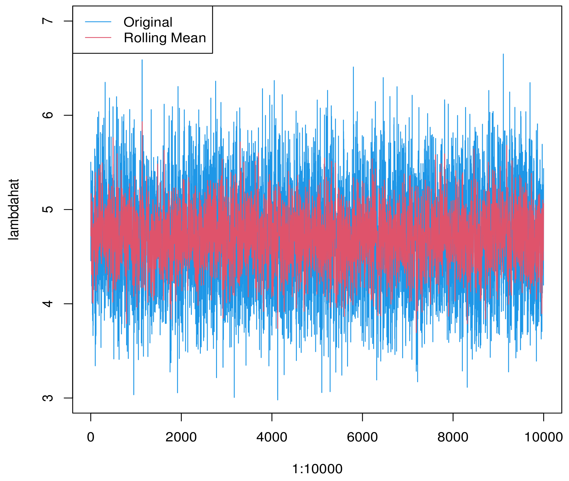
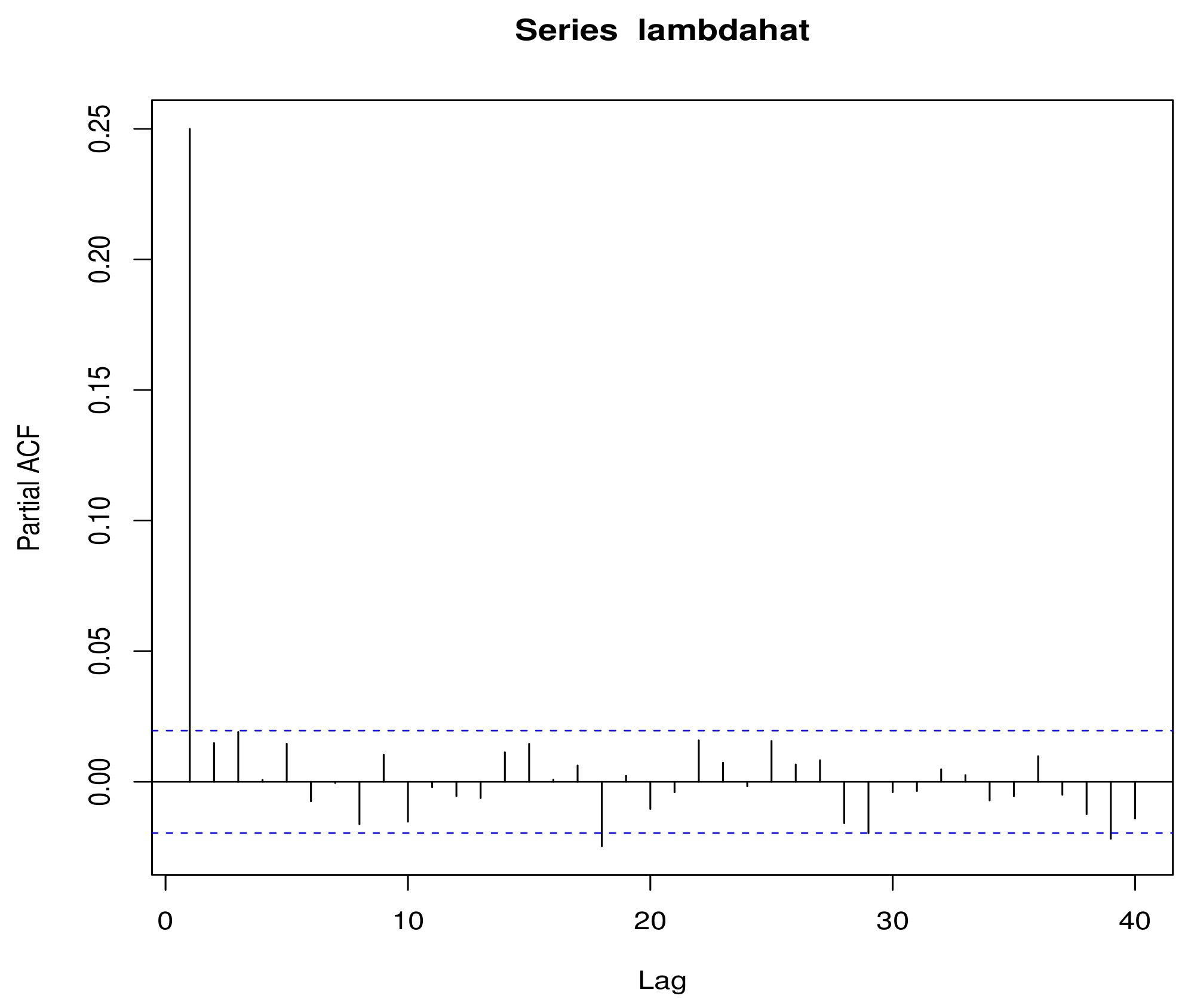
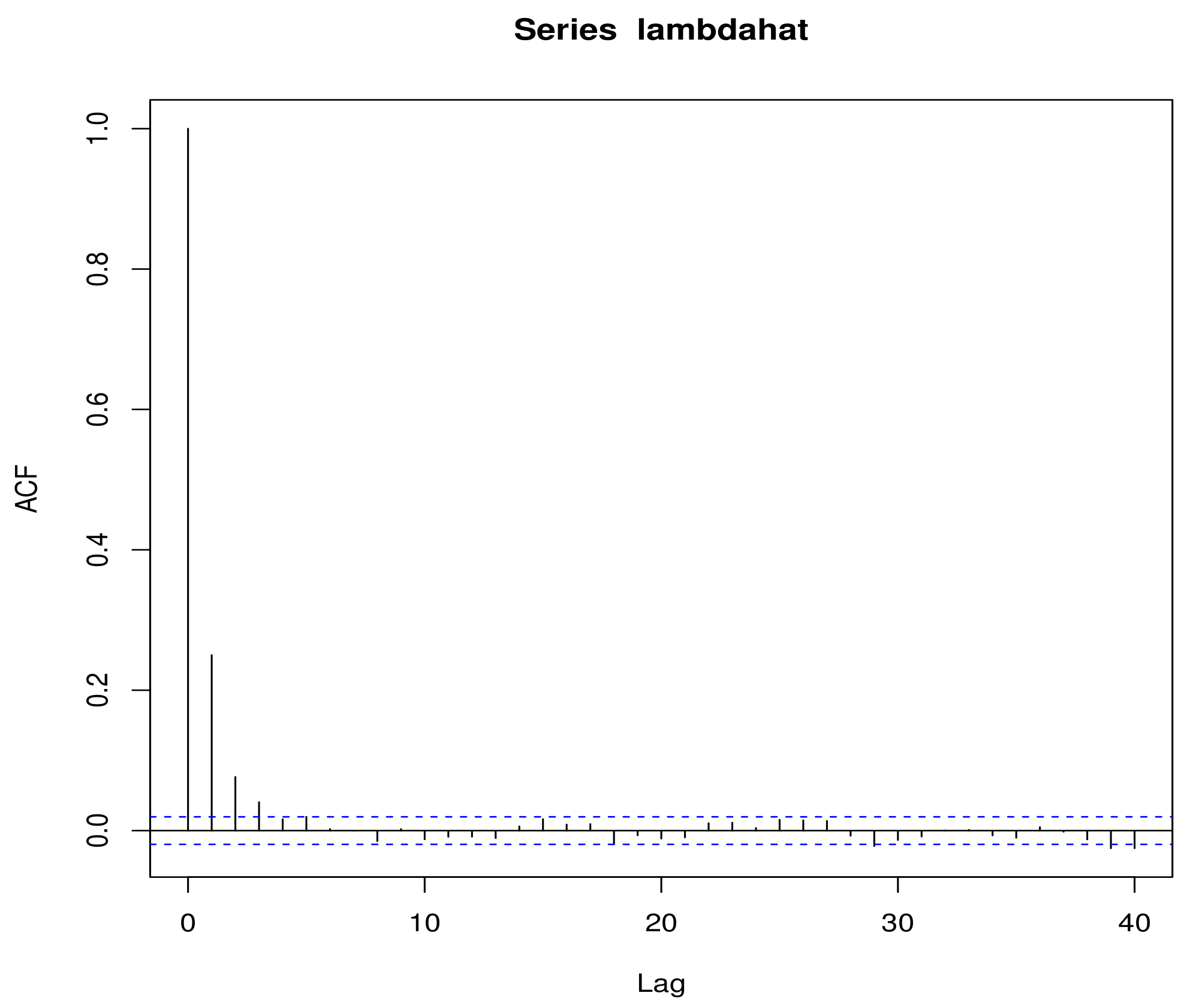
Appendix A. MCMC Outputs
According to Figure A1, we can determine than the sample density of approximately obeys the law of normal distribution. Figure A2, Figure A3 and Figure A4 show the stationarity of the Markov Chain.
Figure A1.
The sample density of when .

Figure A2.
The sequence of white noise in the draws.

Figure A3.
The autocorrelation coefficient of in the draws.

Figure A4.
The partial autocorrelation coefficient of in the draws.

Appendix B. The Robustness of the Simulation with Different h
Table A1 and Table A2 show that the difference of estimations between different h values is relatively small, and the results still follow the statistical inference discussed above. Therefore, the robustness of the simulations with different h values is verified.

Table A1.
Estimates of parameter for different loss functions when and .
| n | T | c | |||||||||
|---|---|---|---|---|---|---|---|---|---|---|---|
| 50 | (40,30) | 0.2 | 0.5 | 2.6054 | 0.2292 | 2.5742 | 0.2245 | 2.3134 | 0.3251 | 2.2878 | 0.3166 |
| 0.4 | 2.5541 | 0.1832 | 2.5287 | 0.1801 | 2.3135 | 0.2450 | 2.2920 | 0.2399 | |||
| 80 | (60,40) | 0.2 | 2.5796 | 0.1665 | 2.5567 | 0.1640 | 2.3585 | 0.2193 | 2.3387 | 0.2152 | |
| 0.4 | 2.5377 | 0.1142 | 2.5217 | 0.1130 | 2.3804 | 0.1402 | 2.3661 | 0.1384 | |||
| 120 | (90,60) | 0.2 | 2.5481 | 0.1085 | 2.5329 | 0.1074 | 2.3981 | 0.1324 | 2.3844 | 0.1308 | |
| 0.4 | 2.5221 | 0.0751 | 2.5115 | 0.0745 | 2.4158 | 0.0867 | 2.4060 | 0.0860 | |||
| 50 | (40,30) | 0.2 | 1 | 2.6092 | 0.2299 | 2.5779 | 0.2251 | 2.3164 | 0.3262 | 2.2908 | 0.3177 |
| 0.4 | 2.5552 | 0.1833 | 2.5298 | 0.1802 | 2.3145 | 0.2451 | 2.2930 | 0.2401 | |||
| 80 | (60,40) | 0.2 | 2.5645 | 0.1646 | 2.5418 | 0.1621 | 2.3457 | 0.2163 | 2.3261 | 0.2123 | |
| 0.4 | 2.5385 | 0.1143 | 2.5226 | 0.1131 | 2.3812 | 0.1403 | 2.3668 | 0.1385 | |||
| 120 | (90,60) | 0.2 | 2.5523 | 0.1089 | 2.5371 | 0.1078 | 2.4018 | 0.1329 | 2.3881 | 0.1313 | |
| 0.4 | 2.5243 | 0.0752 | 2.5137 | 0.0747 | 2.4179 | 0.0869 | 2.4080 | 0.0862 | |||
| 50 | (40,30) | 0.2 | 1.5 | 2.6017 | 0.2285 | 2.5706 | 0.2238 | 2.3105 | 0.3237 | 2.2850 | 0.3153 |
| 0.4 | 2.5570 | 0.1835 | 2.5316 | 0.1805 | 2.3161 | 0.2456 | 2.2945 | 0.2406 | |||
| 80 | (60,40) | 0.2 | 2.5778 | 0.1663 | 2.5548 | 0.1638 | 2.3569 | 0.2190 | 2.3372 | 0.2150 | |
| 0.4 | 2.5392 | 0.1144 | 2.5233 | 0.1132 | 2.3818 | 0.1404 | 2.3675 | 0.1386 | |||
| 120 | (90,60) | 0.2 | 2.5416 | 0.1080 | 2.5266 | 0.1069 | 2.3924 | 0.1316 | 2.3788 | 0.1300 | |
| 0.4 | 2.5258 | 0.0752 | 2.5153 | 0.0747 | 2.4193 | 0.0869 | 2.4095 | 0.0863 |
Table A2.
Estimates of parameter for different loss functions when and .
| n | T | c | |||||||||
|---|---|---|---|---|---|---|---|---|---|---|---|
| 50 | (40,30) | 0.2 | 0.5 | 2.6014 | 0.2285 | 2.5703 | 0.2238 | 2.5460 | 0.2320 | 2.5160 | 0.2272 |
| 0.4 | 2.5572 | 0.1835 | 2.5318 | 0.1804 | 2.5124 | 0.1857 | 2.4877 | 0.1825 | |||
| 80 | (60,40) | 0.2 | 2.5721 | 0.1656 | 2.5493 | 0.1631 | 2.5316 | 0.1674 | 2.5094 | 0.1648 | |
| 0.4 | 2.5373 | 0.1142 | 2.5213 | 0.1130 | 2.5092 | 0.1150 | 2.4935 | 0.1138 | |||
| 120 | (90,60) | 0.2 | 2.5559 | 0.1092 | 2.5407 | 0.1081 | 2.5290 | 0.1100 | 2.5140 | 0.1088 | |
| 0.4 | 2.5281 | 0.0754 | 2.5175 | 0.0748 | 2.5095 | 0.0757 | 2.4990 | 0.0752 | |||
| 50 | (40,30) | 0.2 | 1 | 2.6168 | 0.2312 | 2.5854 | 0.2265 | 2.5607 | 0.2348 | 2.5304 | 0.2299 |
| 0.4 | 2.5595 | 0.1837 | 2.5341 | 0.1806 | 2.5146 | 0.1859 | 2.4900 | 0.1827 | |||
| 80 | (60,40) | 0.2 | 2.5747 | 0.1659 | 2.5519 | 0.1634 | 2.5342 | 0.1677 | 2.5119 | 0.1651 | |
| 0.4 | 2.5361 | 0.1141 | 2.5201 | 0.1129 | 2.5079 | 0.1150 | 2.4923 | 0.1137 | |||
| 120 | (90,60) | 0.2 | 2.5527 | 0.1089 | 2.5376 | 0.1078 | 2.5259 | 0.1097 | 2.5110 | 0.1086 | |
| 0.4 | 2.5216 | 0.0750 | 2.5111 | 0.0745 | 2.5030 | 0.0754 | 2.4926 | 0.0748 | |||
| 50 | (40,30) | 0.2 | 1.5 | 2.6069 | 0.2297 | 2.5757 | 0.2249 | 2.5512 | 0.2332 | 2.5211 | 0.2283 |
| 0.4 | 2.5543 | 0.1831 | 2.5290 | 0.1801 | 2.5096 | 0.1853 | 2.4850 | 0.1821 | |||
| 80 | (60,40) | 0.2 | 2.5765 | 0.1661 | 2.5536 | 0.1636 | 2.5359 | 0.1679 | 2.5136 | 0.1653 | |
| 0.4 | 2.5309 | 0.1138 | 2.5149 | 0.1126 | 2.5028 | 0.1146 | 2.4872 | 0.1134 | |||
| 120 | (90,60) | 0.2 | 2.5459 | 0.1084 | 2.5308 | 0.1073 | 2.5192 | 0.1091 | 2.5044 | 0.1080 | |
| 0.4 | 2.5283 | 0.0754 | 2.5177 | 0.0749 | 2.5096 | 0.0757 | 2.4991 | 0.0752 |
Appendix C. MCMC Method for Two Unknown Parameters
| Algorithm A1 The MCMC algorithm for two unknown parameters. |
|
References
- Chen, Z. A new two-parameter lifetime distribution with bathtub shape or increasing failure rate function. Stat. Probab. Lett. 2008, 49, 155–161. [Google Scholar] [CrossRef]
- Hjorth, U. A reliability distribution with increasing, decreasing, and bathtub-shaped failure rate data. Technometrics 1980, 22, 99–107. [Google Scholar] [CrossRef]
- Mudholkar, G.S.; Srivastava, D.K. Exponentiated Weibull family for analyzing bathtub failure-rate data. IEEE Trans. Reliab. 1993, 42, 299–302. [Google Scholar] [CrossRef]
- Sarhan, A.M.; Hamilton, D.C.; Smith, B. Parameter estimation for a two-parameter bathtub-shaped lifetime distribution. Appl. Math. Model. 2012, 36, 5380–5392. [Google Scholar] [CrossRef]
- Wu, S. Estimation of the two-parameter bathtub-shaped lifetime distribution with progressive censoring. J. Appl. Stat. 2008, 35, 1139–1150. [Google Scholar] [CrossRef]
- Rastogi, M.K.; Tripathi, Y.M. Estimation using hybrid censored data from a two-parameter distribution with bathtub shape. Comput. Stat. Data Anal. 2013, 67, 268–281. [Google Scholar] [CrossRef]
- Smith, R.M.; Bain, L.J. An Exponential Power Life-Testing Distribution. Commun. Stat. Theory Methods 1975, 4, 469–481. [Google Scholar]
- Epstein, B. Truncated Life Tests in the Exponential Case. Ann. Math. Stat. 1954, 25, 555–564. [Google Scholar] [CrossRef]
- Chandrasekar, B.; Childs, A.; Balakrishnan, N. Exact Likelihood Inference for the Exponential Distribution under Generalized Type-I and Type-II Hybrid Censoring. Nav. Res. Logist. 2004, 51, 994–1004. [Google Scholar] [CrossRef]
- Balakrishnan, N.; Kundu, D. Hybrid censoring: Models, inferential results and applications. Comput. Stat. Data Anal. 2013, 57, 166–209. [Google Scholar] [CrossRef]
- Rabie, A.; Li, J. E-Bayesian Estimation for Burr-X Distribution Based on Generalized Type-I Hybrid Censoring Scheme. Am. J. Math. Manag. Sci. 2018, 41–55. [Google Scholar] [CrossRef] [Green Version]
- Sen, T.; Bhattacharya, R.; Tripathi, Y.M. Generalized hybrid censored reliability acceptance sampling plans for the Weibull distribution. Am. J. Math. Manag. Sci. 2018, 37, 324–343. [Google Scholar] [CrossRef]
- Nassar, M.; Dobbah, S.A. Analysis of Reliability Characteristics of Bathtub-Shaped Distribution Under Adaptive Type-I Progressive Hybrid Censoring. IEEE Access 2020, 8, 181796–181806. [Google Scholar] [CrossRef]
- Kiapour, A. Bayes, E-Bayes and Robust Bayes Premium Estimation and Prediction under the Squared Log Error Loss Function. J. Iran. Stat. Soc. 2018, 17, 33–47. [Google Scholar] [CrossRef] [Green Version]
- Han, M. The structure of hierarchical prior distribution and its applications. Chin. Oper. Res. Manag. Sci. 1997, 6, 31–40. [Google Scholar]
- Berger, J.O. Statistical Decision Theory and Bayesian Analysis, 2nd ed.; Springer: New York, NY, USA, 1985. [Google Scholar]
- Dziok, J.; Srivastava, H.M. Classes of analytic functions associated with the generalized hypergeometric function. Appl. Math. Comput. 1999, 103, 1–13. [Google Scholar] [CrossRef]
- Lavanya, A.; Alexander, T.L. Estimation of parameters using Lindley’s method. Int. J. Adv. Res. 2016, 4, 1767–1778. [Google Scholar] [CrossRef] [Green Version]
- Kozumi, H.; Kobayashi, G. Gibbs sampling methods for Bayesian quantile regression. J. Stat. Comput. Simul. 2011, 81, 1565–1578. [Google Scholar] [CrossRef] [Green Version]
- Ahmed, E.A. Bayesian estimation based on progressive Type-II censoring from two-parameter bathtub-shaped lifetime model: A Markov chain Monte Carlo approach. J. Appl. Stat. 2014, 41, 752–768. [Google Scholar] [CrossRef]
- Han, M. The E-Bayesian estimation and its E-MSE of Pareto distribution parameter under different loss functions. J. Stat. Comput. Simul. 2020, 90, 1834–1848. [Google Scholar] [CrossRef]
- Lawless, J.F. Statistical models and methods for lifetime data. Publ. Am. Stat. Assoc. 2003, 45, 264–265. [Google Scholar]
Figure 1.
pdf of CHD when .

Figure 2.
pdf of CHD when .

Figure 3.
of CHD when .

Figure 4.
of CHD when .

Figure 5.
of CHD when .

Figure 6.
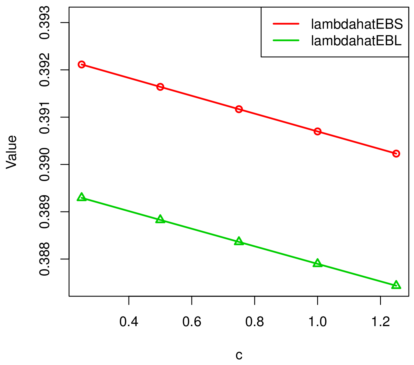
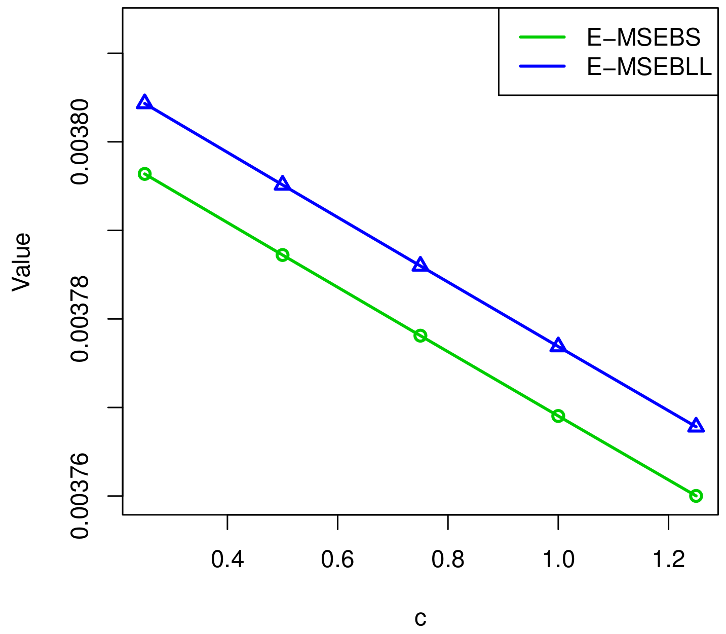
The relationship between c and , .

Figure 7.
The relationship between c and , .

Table 1.
Estimations of under an SE loss function when and .
| n | 50 | 80 | 120 | |||
| (30,40) | (60,40) | (90,60) | ||||
| T | 0.2 | 0.4 | 0.2 | 0.4 | 0.2 | 0.4 |
| 4.4335 | 4.4768 | 4.3911 | 4.4303 | 4.3831 | 4.4187 | |
| 0.6119 | 0.5065 | 0.3862 | 0.3293 | 0.2570 | 0.2179 | |
| min | 1.7563 | 2.5385 | 2.9202 | 2.9999 | 3.4522 | 3.5749 |
| max | 7.1331 | 6.2912 | 5.9283 | 5.7578 | 5.3641 | 5.2460 |
| length | 5.3767 | 3.7527 | 3.0081 | 2.7579 | 1.9120 | 1.6711 |
| n | 50 | 80 | 120 | |||
| (30,40) | (60,40) | (90,60) | ||||
| T | 0.2 | 0.4 | 0.2 | 0.4 | 0.2 | 0.4 |
| 4.3613 | 4.4168 | 4.3447 | 4.3908 | 4.3519 | 4.3923 | |
| 0.5942 | 0.4943 | 0.3790 | 0.3240 | 0.2538 | 0.2155 | |
| min | 2.1555 | 2.5336 | 2.9889 | 3.1245 | 3.3145 | 3.5509 |
| max | 6.3399 | 5.8610 | 5.5518 | 5.4765 | 5.3042 | 5.0982 |
| length | 4.1844 | 3.3274 | 2.5628 | 2.3520 | 1.9897 | 1.5473 |
Table 2.
Estimations of under an SE loss function when and .
| n | 50 | 80 | 120 | |||
| (30,40) | (60,40) | (90,60) | ||||
| T | 0.2 | 0.4 | 0.2 | 0.4 | 0.2 | 0.4 |
| 0.73977 | 0.73287 | 0.74154 | 0.74467 | 0.74416 | 0.74291 | |
| 0.00109 | 0.00088 | 0.00057 | 0.00038 | 0.00019 | 0.00012 | |
| min | 0.61717 | 0.65334 | 0.66958 | 0.67735 | 0.69564 | 0.70122 |
| max | 0.88796 | 0.84219 | 0.82072 | 0.81631 | 0.7917 | 0.78515 |
| length | 0.27079 | 0.18885 | 0.15113 | 0.13895 | 0.09607 | 0.08394 |
| n | 50 | 80 | 120 | |||
| (30,40) | (60,40) | (90,60) | ||||
| T | 0.2 | 0.4 | 0.2 | 0.4 | 0.2 | 0.4 |
| 0.74913 | 0.74328 | 0.74888 | 0.74962 | 0.74867 | 0.74657 | |
| 0.00096 | 0.00077 | 0.00047 | 0.00033 | 0.00017 | 0.00011 | |
| min | 0.65119 | 0.67264 | 0.68686 | 0.69037 | 0.69846 | 0.70826 |
| max | 0.864300 | 0.84247 | 0.81691 | 0.80945 | 0.79911 | 0.78643 |
| length | 0.213100 | 0.16983 | 0.13005 | 0.11908 | 0.10065 | 0.07817 |
Table 3.
Estimations of under a LINEX loss function when and .
| n | 50 | 80 | 120 | |||
| (30,40) | (60,40) | (90,60) | ||||
| T | 0.2 | 0.4 | 0.2 | 0.4 | 0.2 | 0.4 |
| 4.0436 | 4.1358 | 4.1247 | 4.2005 | 4.2009 | 4.2630 | |
| 0.7860 | 0.6341 | 0.4601 | 0.3856 | 0.2911 | 0.2432 | |
| min | 1.2176 | 1.2062 | 2.2857 | 2.5972 | 2.9827 | 3.2330 |
| max | 7.2472 | 7.137 | 5.8513 | 5.6587 | 5.2302 | 5.0823 |
| length | 6.0296 | 5.9308 | 3.5656 | 3.0615 | 2.2475 | 1.8493 |
| n | 50 | 80 | 120 | |||
| (30,40) | (60,40) | (90,60) | ||||
| T | 0.2 | 0.4 | 0.2 | 0.4 | 0.2 | 0.4 |
| 3.9688 | 4.0837 | 4.0831 | 4.1645 | 4.1720 | 4.2382 | |
| 0.7590 | 0.6160 | 0.4502 | 0.3785 | 0.2870 | 0.2403 | |
| min | 0.8753 | 1.5263 | 2.3519 | 2.5144 | 2.9413 | 3.3233 |
| max | 6.3150 | 5.9493 | 5.5490 | 5.6569 | 5.2711 | 5.0406 |
| length | 5.4397 | 4.4230 | 3.1970 | 3.1425 | 2.3298 | 1.7173 |
Table 4.
Estimations of under a LINEX loss function when and .
| n | 50 | 80 | 120 | |||
| (30,40) | (60,40) | (90,60) | ||||
| T | 0.2 | 0.4 | 0.2 | 0.4 | 0.2 | 0.4 |
| 0.76178 | 0.75368 | 0.75179 | 0.75539 | 0.75372 | 0.75066 | |
| 0.00173 | 0.00128 | 0.00073 | 0.00055 | 0.00028 | 0.00016 | |
| min | 0.61242 | 0.61700 | 0.67308 | 0.68191 | 0.70197 | 0.70903 |
| max | 0.92092 | 0.92163 | 0.85672 | 0.83885 | 0.81725 | 0.80353 |
| length | 0.30850 | 0.30463 | 0.18364 | 0.15694 | 0.11529 | 0.09450 |
| n | 50 | 80 | 120 | |||
| (30,40) | (60,40) | (90,60) | ||||
| T | 0.2 | 0.4 | 0.2 | 0.4 | 0.2 | 0.4 |
| 0.77050 | 0.76209 | 0.75857 | 0.76036 | 0.75788 | 0.75433 | |
| 0.00141 | 0.00107 | 0.00064 | 0.00047 | 0.00026 | 0.00015 | |
| min | 0.65229 | 0.66863 | 0.68699 | 0.68199 | 0.70003 | 0.71103 |
| max | 0.94250 | 0.90189 | 0.85289 | 0.84356 | 0.81954 | 0.79863 |
| length | 0.29021 | 0.23325 | 0.16590 | 0.16157 | 0.11952 | 0.08761 |
Table 5.
Estimates of parameter for different loss functions when and .
| n | T | c | |||||||||
|---|---|---|---|---|---|---|---|---|---|---|---|
| 50 | (40,30) | 0.2 | 0.5 | 4.5025 | 0.6847 | 4.4226 | 0.6627 | 4.0575 | 0.9078 | 3.9910 | 0.8723 |
| 0.4 | 4.4863 | 0.6670 | 4.4081 | 0.6462 | 4.0509 | 0.8746 | 3.9856 | 0.8418 | |||
| 80 | (60,40) | 0.2 | 4.4771 | 0.5060 | 4.4172 | 0.4937 | 4.1365 | 0.6330 | 4.0844 | 0.6150 | |
| 0.4 | 4.4097 | 0.4456 | 4.3564 | 0.4360 | 4.1060 | 0.5420 | 4.0590 | 0.5286 | |||
| 120 | (90,60) | 0.2 | 4.4369 | 0.3304 | 4.3972 | 0.3250 | 4.2064 | 0.3870 | 4.1703 | 0.3799 | |
| 0.4 | 4.3957 | 0.2976 | 4.3598 | 0.2933 | 4.1866 | 0.3427 | 4.1536 | 0.3371 | |||
| 50 | (40,30) | 0.2 | 1 | 4.5057 | 0.6857 | 4.4257 | 0.6637 | 4.0601 | 0.9093 | 3.9935 | 0.8738 |
| 0.4 | 4.4867 | 0.6669 | 4.4085 | 0.6462 | 4.0513 | 0.8748 | 3.9860 | 0.8419 | |||
| 80 | (60,40) | 0.2 | 4.4645 | 0.5037 | 4.4049 | 0.4916 | 4.1254 | 0.6303 | 4.0735 | 0.6123 | |
| 0.4 | 4.4041 | 0.4448 | 4.3509 | 0.4353 | 4.1009 | 0.5409 | 4.0540 | 0.5275 | |||
| 120 | (90,60) | 0.2 | 4.4302 | 0.3291 | 4.3907 | 0.3238 | 4.2005 | 0.3852 | 4.1646 | 0.3781 | |
| 0.4 | 4.3878 | 0.2969 | 4.3519 | 0.2926 | 4.1791 | 0.3417 | 4.1462 | 0.3362 | |||
| 50 | (40,30) | 0.2 | 1.5 | 4.4795 | 0.6779 | 4.4003 | 0.6563 | 4.0386 | 0.8973 | 3.9726 | 0.8624 |
| 0.4 | 4.4829 | 0.6657 | 4.4049 | 0.6450 | 4.0484 | 0.8729 | 3.9831 | 0.8401 | |||
| 80 | (60,40) | 0.2 | 4.4681 | 0.5038 | 4.4085 | 0.4917 | 4.1289 | 0.6298 | 4.0770 | 0.6119 | |
| 0.4 | 4.4199 | 0.4470 | 4.3665 | 0.4374 | 4.1152 | 0.5440 | 4.0681 | 0.5305 | |||
| 120 | (90,60) | 0.2 | 4.4341 | 0.3298 | 4.3945 | 0.3245 | 4.2040 | 0.3861 | 4.1680 | 0.3791 | |
| 0.4 | 4.4051 | 0.2986 | 4.3691 | 0.2943 | 4.1953 | 0.3440 | 4.1622 | 0.3384 |
Table 6.
Estimates of parameter for different loss functions when and .
| n | T | c | |||||||||
|---|---|---|---|---|---|---|---|---|---|---|---|
| 50 | (40,30) | 0.2 | 0.5 | 4.5097 | 0.6869 | 4.4295 | 0.6648 | 4.0633 | 0.9114 | 3.9966 | 0.8757 |
| 0.4 | 4.4996 | 0.6837 | 4.4198 | 0.6618 | 4.0552 | 0.9063 | 3.9887 | 0.8709 | |||
| 80 | (60,40) | 0.2 | 4.4523 | 0.5004 | 4.3930 | 0.4884 | 4.1152 | 0.6249 | 4.0637 | 0.6071 | |
| 0.4 | 4.4692 | 0.5041 | 4.4095 | 0.4920 | 4.1298 | 0.6303 | 4.0779 | 0.6123 | |||
| 120 | (90,60) | 0.2 | 4.4306 | 0.3292 | 4.3911 | 0.3239 | 4.2009 | 0.3854 | 4.1649 | 0.3783 | |
| 0.4 | 4.4220 | 0.3280 | 4.3826 | 0.3227 | 4.1931 | 0.3837 | 4.1573 | 0.3767 | |||
| 50 | (40,30) | 0.2 | 1 | 4.5168 | 0.6895 | 4.4363 | 0.6673 | 4.0688 | 0.9161 | 4.0020 | 0.8802 |
| 0.4 | 4.4953 | 0.6826 | 4.4156 | 0.6607 | 4.0515 | 0.9044 | 3.9852 | 0.8691 | |||
| 80 | (60,40) | 0.2 | 4.4642 | 0.5032 | 4.4046 | 0.4910 | 4.1254 | 0.6290 | 4.0736 | 0.6111 | |
| 0.4 | 4.4663 | 0.5038 | 4.4066 | 0.4916 | 4.1271 | 0.6301 | 4.0752 | 0.6121 | |||
| 120 | (90,60) | 0.2 | 4.4228 | 0.3282 | 4.3834 | 0.3229 | 4.1938 | 0.3840 | 4.1580 | 0.3770 | |
| 0.4 | 4.4383 | 0.3306 | 4.3986 | 0.3252 | 4.2077 | 0.3873 | 4.1716 | 0.3802 | |||
| 50 | (40,30) | 0.2 | 1.5 | 4.5030 | 0.6847 | 4.4231 | 0.6628 | 4.0579 | 0.9078 | 3.9914 | 0.8723 |
| 0.4 | 4.4950 | 0.6821 | 4.4154 | 0.6603 | 4.0515 | 0.9033 | 3.9852 | 0.8681 | |||
| 80 | (60,40) | 0.2 | 4.4738 | 0.5053 | 4.4140 | 0.4931 | 4.1336 | 0.6321 | 4.0816 | 0.6140 | |
| 0.4 | 4.4621 | 0.5029 | 4.4025 | 0.4908 | 4.1234 | 0.6289 | 4.0717 | 0.6110 | |||
| 120 | (90,60) | 0.2 | 4.4304 | 0.3292 | 4.3908 | 0.3239 | 4.2007 | 0.3853 | 4.1647 | 0.3782 | |
| 0.4 | 4.4410 | 0.3310 | 4.4013 | 0.3257 | 4.2101 | 0.3879 | 4.1740 | 0.3808 |
Table 7.
Estimates of parameter for different loss functions when and .
| n | T | c | |||||||||
|---|---|---|---|---|---|---|---|---|---|---|---|
| 50 | (40,30) | 0.2 | 0.5 | 2.6002 | 0.2284 | 2.5691 | 0.2237 | 2.443 | 0.2564 | 2.415 | 0.2505 |
| 0.4 | 2.5623 | 0.1843 | 2.5368 | 0.1812 | 2.4334 | 0.2021 | 2.41 | 0.1984 | |||
| 80 | (60,40) | 0.2 | 2.5758 | 0.166 | 2.5529 | 0.1635 | 2.459 | 0.1808 | 2.4378 | 0.1778 | |
| 0.4 | 2.538 | 0.1144 | 2.522 | 0.1131 | 2.4559 | 0.1214 | 2.4408 | 0.1201 | |||
| 120 | (90,60) | 0.2 | 2.549 | 0.1087 | 2.5339 | 0.1076 | 2.4709 | 0.1151 | 2.4565 | 0.1139 | |
| 0.4 | 2.5278 | 0.0753 | 2.5172 | 0.0748 | 2.473 | 0.0784 | 2.4627 | 0.0779 | |||
| 50 | (40,30) | 0.2 | 1 | 2.5973 | 0.2279 | 2.5663 | 0.2232 | 2.4405 | 0.2558 | 2.4125 | 0.25 |
| 0.4 | 2.5545 | 0.1831 | 2.5291 | 0.1801 | 2.4263 | 0.2007 | 2.4031 | 0.1971 | |||
| 80 | (60,40) | 0.2 | 2.5708 | 0.1654 | 2.5479 | 0.1629 | 2.4543 | 0.1801 | 2.4332 | 0.1772 | |
| 0.4 | 2.5338 | 0.114 | 2.5178 | 0.1128 | 2.452 | 0.121 | 2.4369 | 0.1196 | |||
| 120 | (90,60) | 0.2 | 2.5494 | 0.1087 | 2.5342 | 0.1076 | 2.4712 | 0.1151 | 2.4569 | 0.1139 | |
| 0.4 | 2.529 | 0.0754 | 2.5184 | 0.0749 | 2.4741 | 0.0785 | 2.4639 | 0.0779 | |||
| 50 | (40,30) | 0.2 | 1.5 | 2.6051 | 0.2291 | 2.5739 | 0.2244 | 2.4474 | 0.2573 | 2.4194 | 0.2514 |
| 0.4 | 2.5485 | 0.1826 | 2.5232 | 0.1796 | 2.4207 | 0.2001 | 2.3975 | 0.1965 | |||
| 80 | (60,40) | 0.2 | 2.5743 | 0.1658 | 2.5514 | 0.1633 | 2.4575 | 0.1806 | 2.4364 | 0.1777 | |
| 0.4 | 2.5402 | 0.1144 | 2.5243 | 0.1132 | 2.4581 | 0.1215 | 2.443 | 0.1202 | |||
| 120 | (90,60) | 0.2 | 2.5516 | 0.1088 | 2.5364 | 0.1077 | 2.4733 | 0.1153 | 2.4589 | 0.1141 | |
| 0.4 | 2.5217 | 0.075 | 2.5111 | 0.0745 | 2.467 | 0.0781 | 2.4569 | 0.0776 |
Table 8.
Estimates of parameter for different loss functions when and .
| n | T | c | |||||||||
|---|---|---|---|---|---|---|---|---|---|---|---|
| 50 | (40,30) | 0.2 | 0.5 | 2.6032 | 0.2288 | 2.5720 | 0.2240 | 2.4457 | 0.2568 | 2.4177 | 0.2510 |
| 0.4 | 2.6071 | 0.2298 | 2.5758 | 0.2250 | 2.4490 | 0.2583 | 2.4209 | 0.2524 | |||
| 80 | (60,40) | 0.2 | 2.5813 | 0.1683 | 2.5581 | 0.1657 | 2.4629 | 0.1838 | 2.4415 | 0.1807 | |
| 0.4 | 2.5817 | 0.1682 | 2.5586 | 0.1656 | 2.4634 | 0.1835 | 2.4420 | 0.1805 | |||
| 120 | (90,60) | 0.2 | 2.5466 | 0.1088 | 2.5315 | 0.1077 | 2.4684 | 0.1154 | 2.4540 | 0.1141 | |
| 0.4 | 2.5556 | 0.1096 | 2.5403 | 0.1085 | 2.4768 | 0.1163 | 2.4623 | 0.1150 | |||
| 50 | (40,30) | 0.2 | 1 | 2.5997 | 0.2283 | 2.5686 | 0.2236 | 2.4426 | 0.2562 | 2.4146 | 0.2504 |
| 0.4 | 2.6085 | 0.2299 | 2.5773 | 0.2252 | 2.4503 | 0.2583 | 2.4222 | 0.2524 | |||
| 80 | (60,40) | 0.2 | 2.5714 | 0.1670 | 2.5484 | 0.1645 | 2.4539 | 0.1823 | 2.4326 | 0.1792 | |
| 0.4 | 2.5718 | 0.1670 | 2.5487 | 0.1644 | 2.4543 | 0.1821 | 2.4330 | 0.1791 | |||
| 120 | (90,60) | 0.2 | 2.5544 | 0.1095 | 2.5391 | 0.1084 | 2.4756 | 0.1162 | 2.4612 | 0.1149 | |
| 0.4 | 2.5541 | 0.1094 | 2.5389 | 0.1083 | 2.4754 | 0.1160 | 2.4610 | 0.1148 | |||
| 50 | (40,30) | 0.2 | 1.5 | 2.5966 | 0.2279 | 2.5655 | 0.2232 | 2.4397 | 0.2560 | 2.4118 | 0.2501 |
| 0.4 | 2.6042 | 0.2294 | 2.5730 | 0.2246 | 2.4464 | 0.2578 | 2.4183 | 0.2519 | |||
| 80 | (60,40) | 0.2 | 2.5766 | 0.1678 | 2.5535 | 0.1652 | 2.4586 | 0.1831 | 2.4373 | 0.1801 | |
| 0.4 | 2.5842 | 0.1687 | 2.5610 | 0.1661 | 2.4655 | 0.1843 | 2.4441 | 0.1812 | |||
| 120 | (90,60) | 0.2 | 2.5479 | 0.1089 | 2.5327 | 0.1078 | 2.4696 | 0.1155 | 2.4552 | 0.1142 | |
| 0.4 | 2.5490 | 0.1090 | 2.5339 | 0.1079 | 2.4707 | 0.1156 | 2.4563 | 0.1143 |
Table 9.
Estimates of parameter for different loss functions when and .
| n | T | c | |||||||||
|---|---|---|---|---|---|---|---|---|---|---|---|
| 50 | (40,30) | 0.2 | 0.5 | 2.6063 | 0.2295 | 2.5750 | 0.2247 | 2.4484 | 0.2578 | 2.4203 | 0.2519 |
| 0.4 | 2.6006 | 0.2286 | 2.5695 | 0.2239 | 2.4433 | 0.2568 | 2.4153 | 0.2509 | |||
| 80 | (60,40) | 0.2 | 2.5750 | 0.1675 | 2.5519 | 0.1649 | 2.4572 | 0.1827 | 2.4359 | 0.1797 | |
| 0.4 | 2.5793 | 0.1681 | 2.5562 | 0.1655 | 2.4611 | 0.1835 | 2.4398 | 0.1805 | |||
| 120 | (90,60) | 0.2 | 2.5610 | 0.1101 | 2.5456 | 0.1090 | 2.4818 | 0.1168 | 2.4673 | 0.1155 | |
| 0.4 | 2.5565 | 0.1097 | 2.5412 | 0.1086 | 2.4776 | 0.1163 | 2.4632 | 0.1151 | |||
| 50 | (40,30) | 0.2 | 1 | 2.6065 | 0.2296 | 2.5753 | 0.2249 | 2.4485 | 0.2581 | 2.4204 | 0.2522 |
| 0.4 | 2.6147 | 0.2311 | 2.5833 | 0.2263 | 2.4558 | 0.2598 | 2.4275 | 0.2538 | |||
| 80 | (60,40) | 0.2 | 2.5758 | 0.1675 | 2.5527 | 0.1650 | 2.4579 | 0.1828 | 2.4366 | 0.1798 | |
| 0.4 | 2.5810 | 0.1682 | 2.5579 | 0.1656 | 2.4627 | 0.1836 | 2.4413 | 0.1806 | |||
| 120 | (90,60) | 0.2 | 2.5532 | 0.1094 | 2.5379 | 0.1083 | 2.4746 | 0.1160 | 2.4601 | 0.1147 | |
| 0.4 | 2.5505 | 0.1091 | 2.5353 | 0.1080 | 2.4721 | 0.1157 | 2.4577 | 0.1145 | |||
| 50 | (40,30) | 0.2 | 1.5 | 2.6066 | 0.2296 | 2.5753 | 0.2249 | 2.4485 | 0.2581 | 2.4204 | 0.2522 |
| 0.4 | 2.6105 | 0.2306 | 2.5792 | 0.2258 | 2.4519 | 0.2593 | 2.4237 | 0.2534 | |||
| 80 | (60,40) | 0.2 | 2.5752 | 0.1673 | 2.5522 | 0.1648 | 2.4575 | 0.1826 | 2.4362 | 0.1795 | |
| 0.4 | 2.5788 | 0.1680 | 2.5557 | 0.1654 | 2.4607 | 0.1833 | 2.4393 | 0.1803 | |||
| 120 | (90,60) | 0.2 | 2.5443 | 0.1086 | 2.5291 | 0.1075 | 2.4662 | 0.1151 | 2.4518 | 0.1139 | |
| 0.4 | 2.5531 | 0.1094 | 2.5378 | 0.1083 | 2.4745 | 0.1160 | 2.4600 | 0.1147 |
Table 10.
Real data set of 60 observations of electrical appliances.
| 0.014 | 0.034 | 0.059 | 0.061 | 0.069 | 0.080 | 0.123 | 0.142 | 0.165 | 0.210 |
| 0.381 | 0.464 | 0.479 | 0.556 | 0.574 | 0.839 | 0.917 | 0.969 | 0.991 | 1.064 |
| 1.088 | 1.091 | 1.174 | 1.270 | 1.275 | 1.355 | 1.397 | 1.477 | 1.578 | 1.649 |
| 1.702 | 1.893 | 1.932 | 2.001 | 2.161 | 2.292 | 2.326 | 2.337 | 2.628 | 2.785 |
| 2.811 | 2.886 | 2.993 | 3.122 | 3.248 | 3.715 | 3.790 | 3.857 | 3.912 | 4.100 |
| 4.106 | 4.116 | 4.315 | 4.510 | 4.580 | 5.267 | 5.299 | 5.583 | 6.065 | 9.701 |
Table 11.
The results of estimates of for the real data set.
| c | ||||||||
|---|---|---|---|---|---|---|---|---|
| 0.25 | 0.3931 | 0.003801 | 0.3921 | 0.003796 | 0.3903 | 0.003812 | 0.3893 | 0.003804 |
| 0.50 | 0.3931 | 0.003801 | 0.3916 | 0.003787 | 0.3903 | 0.003812 | 0.3888 | 0.003795 |
| 1.00 | 0.3931 | 0.003801 | 0.3912 | 0.003778 | 0.3903 | 0.003812 | 0.3884 | 0.003785 |
| 1.25 | 0.3931 | 0.003801 | 0.3907 | 0.003769 | 0.3903 | 0.003812 | 0.3879 | 0.003776 |
| 1.50 | 0.3931 | 0.003801 | 0.3902 | 0.003759 | 0.3903 | 0.003812 | 0.3874 | 0.003771 |
Table 12.
The results of estimates of for the real data set.
| c | ||||
|---|---|---|---|---|
| 0.25 | 0.730308 | 0.731945 | 0.730892 | 0.732531 |
| 0.50 | 0.730308 | 0.731945 | 0.731185 | 0.732823 |
| 1.00 | 0.730308 | 0.731945 | 0.731419 | 0.733058 |
| 1.25 | 0.730308 | 0.731945 | 0.731711 | 0.733351 |
| 1.50 | 0.730308 | 0.731945 | 0.732004 | 0.733644 |
Publisher’s Note: MDPI stays neutral with regard to jurisdictional claims in published maps and institutional affiliations. |
© 2021 by the authors. Licensee MDPI, Basel, Switzerland. This article is an open access article distributed under the terms and conditions of the Creative Commons Attribution (CC BY) license (https://creativecommons.org/licenses/by/4.0/).
Share and Cite
MDPI and ACS Style
Zhang, Y.; Liu, K.; Gui, W. Bayesian and E-Bayesian Estimations of Bathtub-Shaped Distribution under Generalized Type-I Hybrid Censoring. Entropy 2021, 23, 934. https://doi.org/10.3390/e23080934
AMA Style
Zhang Y, Liu K, Gui W. Bayesian and E-Bayesian Estimations of Bathtub-Shaped Distribution under Generalized Type-I Hybrid Censoring. Entropy. 2021; 23(8):934. https://doi.org/10.3390/e23080934
Chicago/Turabian StyleZhang, Yuxuan, Kaiwei Liu, and Wenhao Gui. 2021. "Bayesian and E-Bayesian Estimations of Bathtub-Shaped Distribution under Generalized Type-I Hybrid Censoring" Entropy 23, no. 8: 934. https://doi.org/10.3390/e23080934
Note that from the first issue of 2016, this journal uses article numbers instead of page numbers. See further details here.