Expressions of forward starting option price in Hull–White stochastic volatility model

Abstract

We are interested in problems related to forward starting options for Hull–White stochastic volatility model. Our objective is to obtain analytical, semi-analytical, or approximated expressions of its price for simulation. To obtain an analytical representation of the price, we use Yor’s formula. However, the analytical formula is difficult to implement. Next we consider semi-analytical expressions for the price. In order to have them, we use the tower property for conditional expectations with a certain filtration and explicitly calculate it. Then, we consider an expansion expression for the price using the semi-analytical expression to have a simple expression. The semi-analytical expressions and the expansion expression can reduce computational costs and standard errors when the Monte Carlo method is used. Finally, some numerical results are given to show their accuracy and efficiency.

Appendices

Greeks of the forward starting option

1.1 Greeks based on first semi-analytical expression

In this subsection, we calculate Greeks based on the first semi-analytical expression given in Theorem 2.

1.1.1 Delta

In this subsection, we give expressions of delta which are calculated based on Theorem 2.

Lemma 3

• (i) $\frac{\partial d^{(2),1}_{s,t}}{\partial S_s} = \frac{\partial d^{(2),2}_{s,t}}{\partial S_s} = \frac{1}{S_s\sqrt{V^{(2)}_{s,t}}}$ holds.

• (ii) For $0\le s<t$ and $i=1,2$, ${\mathrm {e}}^{\theta ^{(i)}_{s,t}}n\left( d^{(i),1}_{s,t} \right) =K^i_{s,t^*}n\left( d^{(i),2}_{s,t} \right)$ holds, where $K^1_{s,u}:=k$ and $K^2_{s,u}:=k\frac{S_u}{S_s}$ and $n(x):=\frac{1}{\sqrt{2\pi }}{\mathrm {e}}^{-\frac{x^2}{2}}$.

From the definition of $d^{(2),i}_{s,t}$ for $i=1,2$, the result follows.

Proposition 4

We have the following expressions for delta:

• (i) For $0\le t\le t^*<T$, we have

  $$\begin{aligned} \frac{\partial C_{FWS}}{\partial S_t}(t,\sigma _t,S_t) = {\mathrm {e}}^{-r(T-t)}E^Q\left[ \left. F^{(1)}_{t^*,T}\frac{S_{t^*}}{S_t} \right| {{\mathcal {F}}}_t \right] = \frac{C_{FWS}(t,\sigma _t,S_t)}{S_t}. \end{aligned}$$

• (ii) For $0\le t^*\le t<T$, we have

  $$\begin{aligned} \frac{\partial C_{FWS}}{\partial S_t}(t,\sigma _t,S_t) = E^Q\left[ \left. {\mathrm {e}}^{\theta ^{(2)}_{t,T}-r(T-t)}N\left( d^{(2),1}_{t,T} \right) \right| {{\mathcal {F}}}_t \right] . \end{aligned}$$

Proof

• (i) As mentioned in Remark 2, when $0\le t\le t^*$, $S_t$ linearly relates to the option price and $F^{(1)}_{t^*,T}$ does not depend on $S_t$. Furthermore, $\frac{\partial S_{t^*}}{\partial S_t}={\mathrm {e}}^{X^{(1)}_{t,t^*}}=\frac{S_{t^*}}{S_t}$; hence, we can obtain (i).

• (ii) From expression of Proposition 1 (ii) and Lemma 3, we have

  $$\begin{aligned} \frac{\partial F^{(2)}_{t,T}}{\partial S_t}= & {} {\mathrm {e}}^{\theta ^{(2)}_{t,T}}n\left( d^{(2),1}_{t,T} \right) \frac{\partial d^{(2),1}_{t,T}}{\partial S_t} + k \frac{S_{t^*}}{S^2_t} N\left( d^{(2),2}_{t,T} \right) - k \frac{S_{t^*}}{S_t} n\left( d^{(2),2}_{t,T} \right) \frac{\partial d^{(2),2}_{t,T}}{\partial S_t} \\= & {} k \frac{S_{t^*}}{S^2_t} N\left( d^{(2),2}_{t,T} \right) . \end{aligned}$$

  And from expression of Theorem 2 (ii), we have

  $$\begin{aligned} \frac{\partial C_{FWS}}{\partial S_t}(t,\sigma _t,S_t)&= {\mathrm {e}}^{-r(T-t)}E^Q\left[ \left. F^{(2)}_{t,T} + S_t\frac{\partial F^{(2)}_{t,T}}{\partial S_t} \right| {{\mathcal {F}}}_t \right] = E^Q\left[ \left. {\mathrm {e}}^{\theta ^{(2)}_{t,T}-r(T-t)}N\left( d^{(2),1}_{t,T} \right) \right| {{\mathcal {F}}}_t \right] . \end{aligned}$$

  $\square$

1.1.2 Gamma

In this subsection, we give expressions for gamma which are calculated based on Theorem 2.

Proposition 5

We have the following expressions for gamma:

• (i) For $0\le t\le t^*<T$, we have $\frac{\partial ^2 C_{FWS}}{\partial S^2_t}(t,\sigma _t,S_t) = 0$.

• (ii) For $0\le t^*\le t<T$, we have

  $$\begin{aligned} \frac{\partial ^2 C_{FWS}}{\partial S^2_t}(t,\sigma _t,S_t)= & {} E^Q\left[ \left. \frac{{\mathrm {e}}^{\theta ^{(2)}_{t,T}-r(T-t)}}{S_t\sqrt{V^{(2)}_{t,T}}}n\left( d^{(2),1}_{t,T} \right) \right| {{\mathcal {F}}}_t \right] \\= & {} E^Q\left[ \left. \frac{kS_{t^*}{\mathrm {e}}^{-r(T-t)}}{S^2_t\sqrt{V^{(2)}_{t,T}}}n\left( d^{(2),2}_{t,T} \right) \right| {{\mathcal {F}}}_t \right] . \end{aligned}$$

Proof

As mentioned in Remark 2, when $0\le t\le t^*$, $S_t$ linearly relates the option price $C_{FWS}$, hence we have (i). From expression (ii) of Proposition 4 and Lemma 3, we have the conclusion (ii). $\square$

1.1.3 Vega

In this subsection, we give expressions of vega which are calculated based on Theorem 2. Note that from the expression of $\sigma _t$ under Q, we have

$$\begin{aligned} \frac{\partial \sigma _t}{\partial \sigma _s}=\exp \left( \left( a-\frac{b^2}{2}\right) (t-s)+b(w_2(t)-w_2(s)) \right) = \frac{\sigma _t}{\sigma _s} \end{aligned}$$

for $0\le s<t$. Using this fact, we have the following lemma.

Lemma 4

For $0\le v\le s<t$ and $i=1,2$, we have the following relations: under Q,

$$\begin{aligned} \frac{\partial S_t}{\partial \sigma _v}= & {} S_t \frac{\partial X^{(i)}_{s,t}}{\partial \sigma _v}, \\ \frac{\partial X^{(i)}_{s,t}}{\partial \sigma _v}= & {} \frac{1}{\sigma _v}\left( \int ^t_s \sigma _u e^{\top } \mathrm{d}w(u) - \int ^t_s \sigma ^2_u \mathrm{d}u \right) , \\ \frac{\partial m^{(i)}_{s,t}}{\partial \sigma _v}= & {} \frac{1}{\sigma _v}\left( \rho \int ^t_s \sigma _u\mathrm{d}w_2(u) - \int ^t_s \sigma ^2_u \mathrm{d}u \right) , \\ \frac{\partial V^{(i)}_{s,t}}{\partial \sigma _v}= & {} \frac{2(1-\rho ^2)}{\sigma _v} \int ^t_s \sigma ^2_u \mathrm{d}u = \frac{2}{\sigma _v}V^{(i)}_{s,t}, \\ \frac{\partial \theta ^{(i)}_{s,t}}{\partial \sigma _v}= & {} \frac{\rho }{\sigma _v}\left( \int ^t_s \sigma _u\mathrm{d}w_2(u) - \rho \int ^t_s \sigma ^2_u \mathrm{d}u \right) , \\ \frac{\partial d^{(i),2}_{s,t}}{\partial \sigma _v}= & {} \frac{-\frac{1}{2}\int ^t_s \sigma ^2_u \mathrm{d}u -r(t-s) + \log K^i_{s,t^*}}{\sigma _v \sqrt{V^{(i)}_{s,t}}}, \\ \frac{\partial d^{(i),1}_{s,t}}{\partial \sigma _v}= & {} \frac{\partial d^{(i),2}_{s,t}}{\partial \sigma _v} + \frac{\sqrt{V^{(i)}_{s,t}}}{\sigma _v}. \end{aligned}$$

Next we consider the derivative $F^{(i)}_{s,t}$, which has been obtained in Proposition 1, in $\sigma _s$.

Proposition 6

For $0\le v\le s< t$ and $i=1,2$, we have

$$\begin{aligned} \frac{\partial F^{(i)}_{s,t}}{\partial \sigma _v} = {\mathrm {e}}^{\theta ^{(i)}_{s,t}}N\left( d^{(i),1}_{s,t} \right) \frac{\partial \theta ^{(i)}_{s,t}}{\partial \sigma _v} + \frac{\sqrt{V^{(i)}_{s,t}}}{\sigma _v}{\mathrm {e}}^{\theta ^{(i)}_{s,t}}n\left( d^{(i),1}_{s,t} \right) . \end{aligned}$$

Remark 7

From Lemma 3, the second term of Proposition 6 can be replaced by $\frac{\sqrt{V^{(i)}_{s,t}}}{\sigma _v}K^i_{s,t^*}n\left( d^{(i),2}_{s,t} \right)$.

Proof

From Proposition 1, we have

$$\begin{aligned} \frac{\partial F^{(i)}_{s,t}}{\partial \sigma _v} =&{\mathrm {e}}^{\theta ^{(i)}_{s,t}}N\left( d^{(i),1}_{s,t} \right) \frac{\partial \theta ^{(i)}_{s,t}}{\partial \sigma _v} + {\mathrm {e}}^{\theta ^{(i)}_{s,t}}n\left( d^{(i),1}_{s,t} \right) \frac{\partial d^{(i),1}_{s,t}}{\partial \sigma _v} - K^i_{s,t^*}n\left( d^{(i),2}_{s,t} \right) \frac{\partial d^{(i),2}_{s,t}}{\partial \sigma _v} \end{aligned}$$

From Lemmas 4 and 3, we have our conclusion. $\square$

Finally, we have the following expression for vega.

Proposition 7

We have the following formulas:

• (i) For $0\le t\le t^*<T$, we have

  $$\begin{aligned} \frac{\partial C_{FWS}}{\partial \sigma _t}(t,\sigma _t,S_t) = {\mathrm {e}}^{-r(T-t)}E^Q\left[ \left. \frac{\partial F^{(1)}_{t^*,T}}{\partial \sigma _t}S_{t^*} + \frac{\partial S_{t^*}}{\partial \sigma _t} F^{(1)}_{t^*,T} \right| {{\mathcal {F}}}_t \right] . \end{aligned}$$

• (ii) For $0\le t^*\le t<T$, we have

  $$\begin{aligned} \frac{\partial C_{FWS}}{\partial \sigma _t}(t,\sigma _t,S_t) = {\mathrm {e}}^{-r(T-t)}S_tE^Q\left[ \left. \frac{\partial F^{(2)}_{t,T}}{\partial \sigma _t} \right| {{\mathcal {F}}}_t \right] . \end{aligned}$$

We can easily derive this proposition from Theorem 2, and each term which appears in each expectation of Proposition 7 is calculated in Lemma 4 and Proposition 6.

1.2 Greeks based on second semi-analytical expression

In this subsection, we calculate Greeks based on the second semi-analytical expression given in Theorem 3.

1.2.1 Delta

In this subsection, another expression of delta is given using the expression provided in Theorem 3.

Proposition 8

For $0\le t\le t^*<T$ and $\rho <0$, we have

$$\begin{aligned} \frac{\partial C_{FWS}}{\partial S_t}(t,\sigma _t,S_t) = {\mathrm {e}}^{-r(T-t^*)}E^{Q^2_{t,t^*}}\left[ \left. F^{(1)}_{t^*,T} \right| {{\mathcal {F}}}_t \right] = \frac{C_{FWS}(t,\sigma _t,S_t)}{S_t}. \end{aligned}$$

$F^{(1)}_{t^*,T}$ does not depend on $S_t$; therefore, from Theorem 3 we obtain this proposition.

Remark 8

As mentioned above, $F^{(1)}_{t^*,T}$ does not depend on $S_t$, so for $0\le t\le t^*<T$, $\frac{\partial C_{FWS}}{\partial S_t}(t,\sigma _t,S_t)$ does not depend on $S_t$, neither. Hence, again we derive that gamma of the option for $0\le t\le t^*<T$ is equal to 0.

1.2.2 Vega

In this subsection, another expression of vega is given using the expression provided in Theorem 3.

Under $Q^2_{s,t}$, we have, for $0\le s<t$ and $0\le v<u$,

$$\begin{aligned} \frac{\partial \sigma _u}{\partial \sigma _v} = 1 + \int ^u_v \left( a + 2\sigma _h\mathbf{1}_{[s,t]}(h) \right) \frac{\partial \sigma _h}{\partial \sigma _v}dh + \int ^u_v b \frac{\partial \sigma _h}{\partial \sigma _v} \mathrm{d}{\tilde{w}}_2(h). \end{aligned}$$

The above equation is linear in $\frac{\partial \sigma _u}{\partial \sigma _v}$, so that we can write the solution as

$$\begin{aligned} \frac{\partial \sigma _u}{\partial \sigma _v} = \exp \left\{ \int ^u_v \left( a + 2\sigma _h\mathbf{1}_{[s,t]}(h) - \frac{b^2}{2} \right) dh + b \left( {\tilde{w}}_2(u)-{\tilde{w}}_2(v) \right) \right\} . \end{aligned}$$

Lemma 5

For $0\le s<t$, $0\le v\le u<x$ and $\rho <0$, we have, under $Q^2_{s,t}$,

Next we consider the derivative $F^{(1)}_{u,x}$, which is obtained in Proposition 1, with respect to $\sigma _s$. The following proposition holds through direct calculations.

Proposition 9

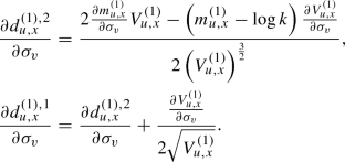
For $0\le s< t$, $0\le v\le u<x$ and $\rho <0$, we have

$$\begin{aligned} \frac{\partial F^{(1)}_{u,x}}{\partial \sigma _v} = {\mathrm {e}}^{\theta ^{(1)}_{u,x}}N\left( d^{(1),1}_{u,x} \right) \frac{\partial \theta ^{(1)}_{u,x}}{\partial \sigma _v} + \frac{\frac{\partial V^{(1)}_{u,x}}{\partial \sigma _v}}{2\sqrt{V^{(1)}_{u,x}}}{\mathrm {e}}^{\theta ^{(1)}_{u,x}}n\left( d^{(1),1}_{u,x} \right) . \end{aligned}$$

Remark 9

Like (ii) of Lemma 3, ${\mathrm {e}}^{\theta ^{(1)}_{u,x}}n\left( d^{(1),1}_{u,x} \right) =kn\left( d^{(1),2}_{u,x} \right)$ holds, so that the second term of Proposition 9 can be replaced by $\frac{\frac{\partial V^{(1)}_{u,x}}{\partial \sigma _v}}{2\sqrt{V^{(1)}_{u,x}}} kn\left( d^{(1),2}_{u,x} \right)$.

Finally, we have the following expression for vega.

Proposition 10

For $0\le t\le t^*<T$ and $\rho <0$, we have

$$\begin{aligned} \frac{\partial C_{FWS}}{\partial \sigma _t}(t,\sigma _t,S_t) = {\mathrm {e}}^{-r(T-t^*)}S_tE^{Q^2_{t,t^*}}\left[ \left. \frac{\partial F^{(1)}_{t^*,T}}{\partial \sigma _t} \right| {{\mathcal {F}}}_t \right] . \end{aligned}$$

Remark 10

One can obtain other Greeks (parameter sensitivities) using similar calculations.

Martingale property of $\frac{S_t}{B_t}$ when $\rho <0$

We will discuss martingale property of $\frac{S_t}{B_t}$ when $\rho <0$.

Recall the following lemma.

Lemma 6

(Hata and Sekine 2006: Lemma 3.1., Hata (2020): Lemma B.1.) For $f:=(f_1,f_2)': (0,\infty ) \mapsto {{{\mathbb {R}}}}^2$, define $f(\sigma ):=\left( f(\sigma _t)\right) _{t\in [0,T]}$. Assume $f(\sigma )$ is progressively measurable such that $\int _0^T |f(\sigma _t)|^2 \mathrm{d}t<\infty$ a.e.. Then, the martingale property of ${{{\mathcal {E}}}} \left( \int f(\sigma )' \mathrm{d}w \right)$ is equivalent to that of ${{{\mathcal {E}}}} \left( \int f_2(\sigma ) \mathrm{d}w_2 \right)$.

Following closely arguments of Lemma B.2 of Hata (2020), we obtain the following lemma at once.

Lemma 7

If $\rho <0$, the process $\displaystyle {\varLambda } _{t}^{\rho }:={{\mathcal {E}}}_t\left( \rho \int _{0}^{(\cdot )} \sigma _{u} \mathrm{d}w_{2}(u)\right)$ is a martingale with mean 1.

Using these lemmas, we have the following.

Lemma 8

If $\rho <0$, $\frac{S_{t}}{B_{t}}$ is a martingale.

Proof

Then, we have

$$\begin{aligned} E\left[ \frac{S_{t}}{B_{t}}\right]= & {} S_0E\left[ {\mathrm {e}}^{\int ^t_0 \sigma _u e^\top \mathrm{d}w(u)-\frac{1}{2}\int ^{t}_{0}\sigma ^{2}_{u}\mathrm{d}u} \right] \\= & {} S_0E\left[ {{\mathcal {E}}}\left( \sqrt{1-\rho ^2} \int _{0}^{(\cdot )}\sigma _{u}\mathrm{d}w_{1}(u) \right) _{t} {{\mathcal {E}}}\left( \rho \int _{0}^{(\cdot )}\sigma _{u}\mathrm{d}w_{2}(u) \right) _{t} \right] \end{aligned}$$

From $\rho <0$ and Lemma 7, we see that ${{\mathcal {E}}}\left( \rho \int _{0}^{(\cdot )}\sigma _{u}\mathrm{d}w_{2}(u) \right) _{t}$ is a martingale. From Lemma 6, $\frac{S_{t}}{B_{t}}$ is a martingale. $\square$

Moreover, we prove the following lemma.

Lemma 9

If $\rho <0$, (10) has a strong solution (11).

Proof

By setting $Z_{t}:=\log \sigma _{t}$, we rewrite (10) as

$$\begin{aligned} \mathrm{d}z_{t}=\left\{ \left( a-\frac{b^{2}}{2}\right) + {\mathrm {e}}^{Z_{t}}\right\} \mathrm{d}t+b\mathrm{d}w^{S}_{2}(t), \qquad Z_{0}=\log \sigma _{0}. \end{aligned}$$

(19)

Since $\rho <0$, (19) has a strong solution:

$$\begin{aligned} Z_{t}&=Z_{0}+bw^{S}_{2}(t)+\left( a-\frac{b^{2}}{2}\right) t-\log \left\{ 1- {\mathrm {e}}^{z_{0}}\int _{0}^{t}{\mathrm {e}}^{bw^{S}_{2}(u)+(a-\frac{b^{2}}{2})u}\mathrm{d}u\right\} . \end{aligned}$$

$\square$

Remark 11

At this moment, it is not so easy to have lemmas from Lemma 7 to Lemma 9 for $\rho >0$ by following our arguments. Even if we can have these lemmas, the explicit expression (11) of $\sigma _t$ may not be applicable since the denominator can be zero.

Proofs of asymptotic expansion

Here we give proofs for Sect. 4.2.

Lemma 10

For $t\le t^*<T$, we have the following relations.

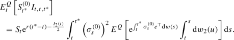
• (i) $\displaystyle {E^Q_t\left[ S^{(0)}_{t^*} I_{t,t,t^*} \right] = {\mathrm {e}}^{r(t^*-t)} S_t \rho I_{2,1}(t).}$

• (ii) For $i=1,2$, $\displaystyle {E^Q_t\left[ S^{(0)}_{t^*} I^{(i)}_{t,t,t^*} \right] = a_i {\mathrm {e}}^{r(t^*-t)} S_t \rho I_{2,1}(t)}$, where $a_1:=\sqrt{1-\rho ^2}$ and $a_2:=\rho$.

• (iii) $\displaystyle {E^Q_t\left[ S^{(0)}_{t^*} (w_2(t^*) - w_2(t)) \right] = {\mathrm {e}}^{r(t^*-t)} S_t \rho I_1(t)}$.

Proof

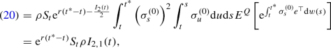
• (i) Due to Proposition 2,

  

  (20)

  For the first term, we use the duality formula in Malliavin calculus (Proposition 3.2.3 in Nualart and Nualart 2018);

  

  where we use Lemma 2 (iv).

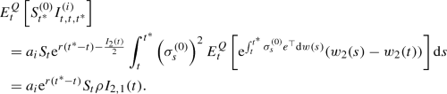
• (ii) From the duality formula in Malliavin calculus and as (i), we have

  

• (iii) As (i), we have

  $$\begin{aligned}&E^Q_t\left[ S^{(0)}_{t^*} (w_2(t^*) - w_2(t)) \right] \\&\quad = \rho S_t {\mathrm {e}}^{r(t^*-t) - \frac{I_2(t)}{2}} \int ^{t^*}_t \sigma ^{(0)}_s \mathrm{d}s E^Q\left[ {\mathrm {e}}^{\int ^{t^*}_t \sigma ^{(0)}_s e^{\top } \mathrm{d}w(s)} \right] \\&\quad = {\mathrm {e}}^{r(t^*-t)} S_t \rho I_1(t). \end{aligned}$$

$\square$

Lemma 11

We have the following equations.

• (i) $\displaystyle {E^Q\left[ {\mathrm {e}}^{\theta ^{(1),(0)}_{t^*,T}}N\left( d^{(1),1,(0)}_{t^*,T}\right) I_{t^*,t^*,T} \right] }$

  $\displaystyle {=I'_{2,1} \left\{ \rho E^Q\left[ {\mathrm {e}}^{{\varTheta } + \rho X} N\left( D_1 + D_3X \right) \right] + D_3 E^Q\left[ {\mathrm {e}}^{{\varTheta } + \rho X}n\left( D_1 + D_3X \right) \right] \right\} }$, where recall that n(x) is the density function of the standard normal distribution.

• (ii) $\displaystyle {E^Q\left[ {\mathrm {e}}^{\theta ^{(1),(0)}_{t^*,T}}N\left( d^{(1),1,(0)}_{t^*,T}\right) I^{(2)}_{t^*,t^*,T} \right] }$

  $\displaystyle {=I'_{2,1} \left\{ \rho ^2 E^Q\left[ {\mathrm {e}}^{{\varTheta } + \rho X} N\left( D_1 + D_3X \right) \right] + 2 \rho D_3 E^Q\left[ {\mathrm {e}}^{{\varTheta } + \rho X}n\left( D_1 + D_3X \right) \right] \right. }$

  $\displaystyle {\left. \quad \quad \quad - D^2_3 E^Q\left[ {\mathrm {e}}^{{\varTheta } + \rho X}n\left( D_1 + D_3X \right) \left( D_1 + D_3X \right) \right] \right\} }$.

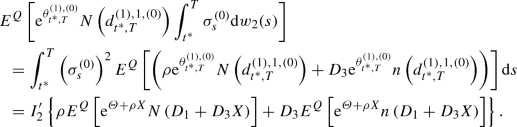
• (iii) $\displaystyle {E^Q\left[ {\mathrm {e}}^{\theta ^{(1),(0)}_{t^*,T}}N\left( d^{(1),1,(0)}_{t^*,T}\right) \int ^T_{t^*} \sigma ^{(0)}_s \mathrm{d}w_2(s) \right] }$

  $\displaystyle {= I'_{2} \left\{ \rho E^Q\left[ {\mathrm {e}}^{{\varTheta } + \rho X} N\left( D_1 + D_3X \right) \right] + D_3 E^Q\left[ {\mathrm {e}}^{{\varTheta } + \rho X}n\left( D_1 + D_3X \right) \right] \right\} }$.

• (iv) $\displaystyle {E^Q\left[ n\left( d^{(1),2,(0)}_{t^*,T}\right) I_{t^*,t^*,T} \right] = - D_3 I'_{2,1} E^Q\left[ n\left( D_2 + D_3 X \right) (D_2 + D_3 X) \right] }$.

• (v) Let a, b be constants and X be a random variable with $N(0,\sigma ^2)$ where $\sigma ^2>0$. We have

  $$\begin{aligned} f(a,b) := E^Q\left[ n(a+bX) \right] = \frac{1}{\sqrt{2\pi (b^2\sigma ^2 + 1)}}\exp \left( -\frac{a^2}{2(b^2\sigma ^2 + 1)} \right) . \end{aligned}$$

  And

  $$\begin{aligned} - \frac{\partial }{\partial a}f(a,b) = E^Q\left[ n(a+bX) (a+bX) \right] = -\frac{a}{b^2\sigma ^2 + 1} f(a,b). \end{aligned}$$

Proof

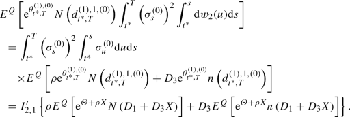
• (i) Due to Lemma 10 and the duality formula in Malliavin calculus, we have

  

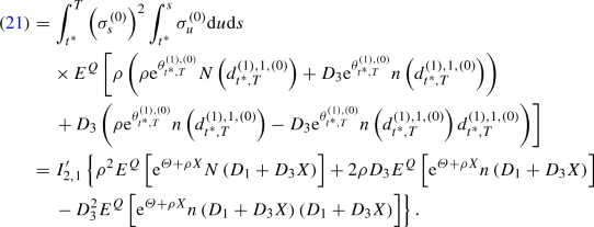
• (ii) From the duality formula in Malliavin calculus, we have

  

  (21)

  Again we use the duality formula in Malliavin calculus;

  

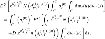
• (iii) From the duality formula in Malliavin calculus, we have

  

• (iv) From the duality formula in Malliavin calculus, we have

  

• (v) Using

  $$\begin{aligned} - \frac{(bx + a)^2}{2} - \frac{x^2}{2\sigma ^2} = - \frac{(x + \frac{ab}{b^2\sigma ^2 + 1}\sigma ^2)^2}{2 \frac{\sigma ^2}{b^2\sigma ^2 + 1}} - \frac{a^2}{2(b^2\sigma ^2 + 1)}, \end{aligned}$$

  we have

  $$\begin{aligned} f(a,b)= & {} \int ^{\infty }_{-\infty } \frac{1}{\sqrt{2\pi }}{\mathrm {e}}^{-\frac{(bx+a)^2}{2}}\frac{1}{\sqrt{2\pi \sigma ^2}}{\mathrm {e}}^{-\frac{x^2}{2\sigma ^2}}\mathrm{d}x \\= & {} \frac{1}{\sqrt{2\pi (b^2\sigma ^2 + 1)}} {\mathrm {e}}^{-\frac{a^2}{2(b^2\sigma ^2 + 1)}} \int ^{\infty }_{-\infty } \frac{1}{\sqrt{2\pi \frac{\sigma ^2}{b^2\sigma ^2 + 1}}} {\mathrm {e}}^{- \frac{(x + \frac{ab}{b^2\sigma ^2 + 1}\sigma ^2)^2}{2 \frac{\sigma ^2}{b^2\sigma ^2 + 1}}} \mathrm{d}x. \end{aligned}$$

  Note that $\int ^{\infty }_{-\infty } \frac{1}{\sqrt{2\pi \frac{\sigma ^2}{b^2\sigma ^2 + 1}}} {\mathrm {e}}^{- \frac{(x + \frac{ab}{b^2\sigma ^2 + 1}\sigma ^2)^2}{2 \frac{\sigma ^2}{b^2\sigma ^2 + 1}}}\mathrm{d}x=1$.

  And we can easily obtain $\frac{\partial }{\partial a}f(a,b)$ by standard calculations.

$\square$

Finally, we show the proof of Proposition 3.

Proof of Proposition 3

Now $g_t(\varepsilon )$ is

$$\begin{aligned} g_t(\varepsilon )= & {} {\mathrm {e}}^{-r(T-t)}E^Q_t\left[ S^{(\varepsilon )}_{t^*}\left\{ {\mathrm {e}}^{\theta ^{(1),(\varepsilon )}_{t^*,T}}N\left( d^{(1),1,(\varepsilon )}_{t^*,T} \right) \right. \right. \\&\left. \left. -\, kN\left( d^{(1),2,(\varepsilon )}_{t^*,T} \right) \right\} \right] . \end{aligned}$$

Then, applying the chain rule, we have

$$\begin{aligned} {\dot{g}}_t(\varepsilon )= & {} {\mathrm {e}}^{-r(T-t)}E^Q_t\left[ {\dot{S}}^{(\varepsilon )}_{t^*}\left\{ {\mathrm {e}}^{\theta ^{(1),(\varepsilon )}_{t^*,T}}N\left( d^{(1),1,(\varepsilon )}_{t^*,T} \right) - kN\left( d^{(1),2,(\varepsilon )}_{t^*,T} \right) \right\} \right. \\&\quad +\, S^{(\varepsilon )}_{t^*} \left\{ {\mathrm {e}}^{\theta ^{(1),(\varepsilon )}_{t^*,T}}{\dot{\theta }}^{(1),(\varepsilon )}_{t^*,T}N\left( d^{(1),1,(\varepsilon )}_{t^*,T} \right) + {\mathrm {e}}^{\theta ^{(1),(\varepsilon )}_{t^*,T}}n\left( d^{(1),1,(\varepsilon )}_{t^*,T} \right) {\dot{d}}^{(1),1,(\varepsilon )}_{t^*,T} \right. \\&\quad \left. \left. -\, kn\left( d^{(1),2,(\varepsilon )}_{t^*,T} \right) {\dot{d}}^{(1),2,(\varepsilon )}_{t^*,T} \right\} \right] . \end{aligned}$$

Note that from Lemma 2 (i), we have, under $S^{(0)}_t=S$ and $\sigma ^{(0)}_t=\sigma$,

$$\begin{aligned} {\dot{S}}^{(0)}_{t^*}= & {} S^{(0)}_{t^*} \left\{ - \int ^{t^*}_t \sigma ^{(0)}_s {\dot{\sigma }}^{(0)}_s \mathrm{d}s + \sqrt{1-\rho ^2} \int ^{t^*}_t {\dot{\sigma }}^{(0)}_s \mathrm{d}w_1(s) + \rho \int ^{t^*}_t {\dot{\sigma }}^{(0)}_s \mathrm{d}w_2(s) \right\} \\= & {} b S^{(0)}_{t^*} \left( - I_{t,t,t^*} + \sqrt{1-\rho ^2} I^{(1)}_{t,t,t^*} + \rho I^{(2)}_{t,t,t^*} \right) , \end{aligned}$$

and similarly, we obtain

$$\begin{aligned} {\dot{\theta }}^{(1),(0)}_{t^*,T}= & {} b \left( - \rho ^2 I_{t,t^*,T} + \rho I^{(2)}_{t,t^*,T} \right) , \\ {\dot{d}}^{(1),1,(0)}_{t^*,T}= & {} b \left\{ \left( \frac{1-2\rho ^2}{\sqrt{(1-\rho ^2)I'_2}} - \frac{d^{(1),1,(0)}_{t^*,T}}{I'_2} \right) I_{t,t^*,T} + \frac{\rho }{\sqrt{(1-\rho ^2)I'_2}} I^{(2)}_{t,t^*,T} \right\} , \\ {\dot{d}}^{(1),2,(0)}_{t^*,T}= & {} b \left\{ \left( \frac{-1}{\sqrt{(1-\rho ^2)I'_2}} - \frac{d^{(1),2,(0)}_{t^*,T}}{I'_2} \right) I_{t,t^*,T} + \frac{\rho }{\sqrt{(1-\rho ^2)I'_2}} I^{(2)}_{t,t^*,T} \right\} . \end{aligned}$$

Then, we have

$$\begin{aligned}&{\dot{g}}_t(0) \nonumber \\&\quad = b{\mathrm {e}}^{-r(T-t)}E^Q_t\left[ S^{(0)}_{t^*} \left\{ {\mathrm {e}}^{\theta ^{(1),(0)}_{t^*,T}}N\left( d^{(1),1,(0)}_{t^*,T}\right) \right. \right. \nonumber \\&\qquad \left. -\, kN\left( d^{(1),2,(0)}_{t^*,T}\right) \right\} \left( - I_{t,t,t^*} + \sqrt{1-\rho ^2} I^{(1)}_{t,t,t^*} + \rho I^{(2)}_{t,t,t^*} \right) \nonumber \\&\qquad +\, S^{(0)}_{t^*} {\mathrm {e}}^{\theta ^{(1),(0)}_{t^*,T}}N\left( d^{(1),1,(0)}_{t^*,T}\right) \left( - \rho ^2 I_{t,t^*,T} + \rho I^{(2)}_{t,t^*,T} \right) \nonumber \\&\qquad +\, S^{(0)}_{t^*} {\mathrm {e}}^{\theta ^{(1),(0)}_{t^*,T}}n\left( d^{(1),1,(0)}_{t^*,T}\right) \left\{ \left( \frac{1-2\rho ^2}{\sqrt{(1-\rho ^2)I'_2}} - \frac{d^{(1),1,(0)}_{t^*,T}}{I'_2} \right) I_{t,t^*,T} + \frac{\rho }{\sqrt{(1-\rho ^2)I'_2}} I^{(2)}_{t,t^*,T} \right\} \nonumber \\&\qquad \left. -\, kS^{(0)}_{t^*}n\left( d^{(1),2,(0)}_{t^*,T}\right) \left\{ \left( \frac{-1}{\sqrt{(1-\rho ^2)I'_2}} - \frac{d^{(1),2,(0)}_{t^*,T}}{I'_2} \right) I_{t,t^*,T} + \frac{\rho }{\sqrt{(1-\rho ^2)I'_2}} I^{(2)}_{t,t^*,T} \right\} \right] . \nonumber \\ \end{aligned}$$

(22)

From independence of $\{(w_1(u),w_2(u))\}_{0\le u\le t^*}$ and $\{(w_1(u),w_2(u))\}_{t^*\le u\le T}$, and

$$\begin{aligned} I_{t,t^*,T}=I_{t^*,t^*,T}+(w_2(t^*)-w_2(t))I'_2, \quad I^{(2)}_{t,t^*,T}=I^{(2)}_{t^*,t^*,T}+(w_2(t^*)-w_2(t))\int ^T_{t^*}\sigma ^{(0)}_s\mathrm{d}w_2(s), \end{aligned}$$

we have

$$\begin{aligned}&(22) \nonumber \\&\quad = b{\mathrm {e}}^{-r(T-t)} \left\{ E^Q_t\left[ S^{(0)}_{t^*} \left\{ - I_{t,t,t^*} + \sqrt{1-\rho ^2} I^{(1)}_{t,t,t^*} + \rho I^{(2)}_{t,t,t^*} \right\} \right] E^Q\left[ {\mathrm {e}}^{\theta ^{(1),(0)}_{t^*,T}}N\left( d^{(1),1,(0)}_{t^*,T}\right) \right. \right. \nonumber \\&\qquad \left. -\, kN\left( d^{(1),2,(0)}_{t^*,T}\right) \right] \nonumber \\&\qquad +\, E^Q_t\left[ S^{(0)}_{t^*} \right] E^Q\left[ {\mathrm {e}}^{\theta ^{(1),(0)}_{t^*,T}}N\left( d^{(1),1,(0)}_{t^*,T}\right) \left( -\rho ^2 I_{t^*,t^*,T} + \rho I^{(2)}_{t^*,t^*,T} \right) \right] \nonumber \\&\qquad +\, E^Q_t\left[ S^{(0)}_{t^*} (w_2(t^*) - w_2(t)) \right] E^Q\left[ {\mathrm {e}}^{\theta ^{(1),(0)}_{t^*,T}}N\left( d^{(1),1,(0)}_{t^*,T}\right) \left\{ -\rho ^2 I'_2 + \rho \int ^T_{t^*} \sigma ^{(0)}_s \mathrm{d}w_2(s) \right\} \right] \nonumber \\&\qquad +\, E^Q_t\left[ S^{(0)}_{t^*} \right] E^Q\left[ {\mathrm {e}}^{\theta ^{(1),(0)}_{t^*,T}}n\left( d^{(1),1,(0)}_{t^*,T}\right) \left\{ \left( \frac{1-2\rho ^2}{\sqrt{(1-\rho ^2)I'_2}} \right. \right. \right. \nonumber \\&\qquad \left. \left. \left. -\, \frac{d^{(1),1,(0)}_{t^*,T}}{I'_2} \right) I_{t^*,t^*,T} + D_3 I^{(2)}_{t^*,t^*,T} \right\} \right] \nonumber \\&\qquad +\, E^Q_t\left[ S^{(0)}_{t^*} (w_2(t^*) - w_2(t)) \right] E^Q\left[ {\mathrm {e}}^{\theta ^{(1),(0)}_{t^*,T}}n\left( d^{(1),1,(0)}_{t^*,T}\right) \left\{ \left( \frac{1-2\rho ^2}{\sqrt{(1-\rho ^2)I'_2}} \right. \right. \right. \nonumber \\&\qquad \left. \left. \left. -\, \frac{d^{(1),1,(0)}_{t^*,T}}{I'_2} \right) I'_2 + D_3 \int ^T_{t^*} \sigma ^{(0)}_s \mathrm{d}w_2(s) \right\} \right] \nonumber \\&\qquad -\, k E^Q_t\left[ S^{(0)}_{t^*} \right] E^Q\left[ n\left( d^{(1),2,(0)}_{t^*,T}\right) \left\{ \left( \frac{-1}{\sqrt{(1-\rho ^2)I'_2}} - \frac{d^{(1),2,(0)}_{t^*,T}}{I'_2} \right) I_{t^*,t^*,T} + D_3 I^{(2)}_{t^*,t^*,T} \right\} \right] \nonumber \\&\qquad \left. -\, k E^Q_t\left[ S^{(0)}_{t^*} (w_2(t^*) - w_2(t)) \right] E^Q\left[ n\left( d^{(1),2,(0)}_{t^*,T}\right) \left\{ \left( \frac{-1}{\sqrt{(1-\rho ^2)I'_2}} - \frac{d^{(1),2,(0)}_{t^*,T}}{I'_2} \right) I'_2 \right. \right. \right. \nonumber \\&\qquad \left. \left. \left. +\, D_3 \int ^T_{t^*} \sigma ^{(0)}_s \mathrm{d}w_2(s) \right\} \right] \right\} . \end{aligned}$$

(23)

Note that from Lemma 10 (i) and (ii), we have

$$\begin{aligned} E^Q_t\left[ S^{(0)}_{t^*} \left\{ - I_{t,t,t^*} + \sqrt{1-\rho ^2} I^{(1)}_{t,t,t^*} + \rho I^{(2)}_{t,t,t^*} \right\} \right] = 0. \end{aligned}$$

From Lemma 11 (i) and (ii), we have

$$\begin{aligned}&E^Q\left[ {\mathrm {e}}^{\theta ^{(1),(0)}_{t^*,T}}N\left( d^{(1),1,(0)}_{t^*,T}\right) \left( -\rho ^2 I_{t^*,t^*,T} + \rho I^{(2)}_{t^*,t^*,T} \right) \right] \\&\quad = \rho I'_{2,1} \left( \rho D_3 E^Q\left[ {\mathrm {e}}^{{\varTheta } + \rho X}n(D_1 + D_3 X) \right] - D^2_3 E^Q\left[ {\mathrm {e}}^{{\varTheta } + \rho X}n(D_1 + D_3 X)(D_1 + D_3 X) \right] \right) , \end{aligned}$$

and from Lemma 11 (iii), we have

$$\begin{aligned}&E^Q\left[ {\mathrm {e}}^{\theta ^{(1),(0)}_{t^*,T}}N\left( d^{(1),1,(0)}_{t^*,T}\right) \left\{ -\rho ^2 I'_2 + \rho \int ^T_{t^*} \sigma ^{(0)}_s \mathrm{d}w_2(s) \right\} \right] \\&\quad = \rho I'_{2} D_3 E^Q\left[ {\mathrm {e}}^{{\varTheta } + \rho X}n\left( D_1 + D_3X \right) \right] . \end{aligned}$$

From the above three relations, Lemma 10 (iii) and Lemma 3 (ii) with $i=1$ and the index (0), we have

$$\begin{aligned}&(23) \nonumber \\&\quad = b{\mathrm {e}}^{-r(T-t)}S_t \left\{ {\mathrm {e}}^{r(t^*-t)} \rho I'_{2,1} \left( \rho D_3 E^Q\left[ {\mathrm {e}}^{{\varTheta } + \rho X}n(D_1 + D_3 X) \right] \right. \right. \nonumber \\&\qquad \left. -\, D^2_3 E^Q\left[ {\mathrm {e}}^{{\varTheta } + \rho X}n(D_1 + D_3 X)(D_1 + D_3 X) \right] \right) \nonumber \\&\qquad +\, {\mathrm {e}}^{r(t^*-t)} \rho ^2 I_1(t) I'_{2} D_3 E^Q\left[ {\mathrm {e}}^{{\varTheta } + \rho X}n\left( D_1 + D_3X \right) \right] \nonumber \\&\qquad +\, k {\mathrm {e}}^{r(t^*-t)} E^Q_t\left[ n\left( d^{(1),2,(0)}_{t^*,T}\right) \left( \frac{2-2\rho ^2}{\sqrt{(1-\rho ^2)I'_2}} - \frac{d^{(1),1,(0)}_{t^*,T} - d^{(1),2,(0)}_{t^*,T}}{I'_2} \right) I_{t^*,t^*,T} \right] \nonumber \\&\qquad \left. +\, k {\mathrm {e}}^{r(t^*-t)} \rho I_1(t) E^Q_t\left[ n\left( d^{(1),2,(0)}_{t^*,T}\right) \left( \frac{2-2\rho ^2}{\sqrt{(1-\rho ^2)I'_2}} - \frac{d^{(1),1,(0)}_{t^*,T} - d^{(1),2,(0)}_{t^*,T}}{I'_2} \right) I'_2 \right] \right\} . \nonumber \\ \end{aligned}$$

(24)

From Lemma 3 (ii) with $i=1$ and the index (0), Lemma 11 (iv) and $d^{(1),1,(0)}_{t^*,T} - d^{(1),2,(0)}_{t^*,T} = \sqrt{I'_2}$, we have

$$\begin{aligned}&(24) \nonumber \\&\quad = k b{\mathrm {e}}^{-r(T-t^*)} S_t \left\{ \rho I'_{2,1} \left( \rho D_3 E^Q\left[ n(D_2 + D_3 X) \right] - D^2_3 E^Q\left[ n(D_2 + D_3 X)(D_1 + D_3 X) \right] \right) \right. \nonumber \\&\qquad +\, \rho ^2 I_1(t) I'_{2} D_3 E^Q\left[ n\left( D_2 + D_3X \right) \right] \nonumber \\&\qquad -\, \frac{2\sqrt{1-\rho ^2} - 1}{\sqrt{I'_2}} D_3 I'_{2,1} E^Q\left[ n\left( D_2 + D_3 X \right) (D_2 + D_3 X) \right] \nonumber \\&\qquad +\, \rho I_1(t) I'_2 \frac{2\sqrt{1-\rho ^2} - 1}{\sqrt{I'_2}} E^Q\left[ n\left( D_2 + D_3 X\right) \right] . \end{aligned}$$

(25)

Finally, from $D_1-D_2=\sqrt{(1-\rho ^2)I'_2}$ and Lemma 11 (v), we have

$$\begin{aligned}&(25) \\&\quad = k b{\mathrm {e}}^{-r(T-t^*)} S_t \\&\qquad \times \left\{ \rho \left( \rho I'_{2,1} D_3 - \sqrt{(1-\rho ^2)I'_2} I'_{2,1} D^2_3 \right. \right. \\&\qquad \left. \left. + \rho I_1(t) I'_{2} D_3 + I_1(t) \sqrt{I'_2} \left( 2\sqrt{1-\rho ^2} - 1\right) \right) E^Q\left[ n(D_2 + D_3 X) \right] \right. \\&\qquad \left. -\, \left( \rho D_3 + \frac{2\sqrt{1-\rho ^2} - 1}{\sqrt{I'_2}} \right) D_3 I'_{2,1} E^Q\left[ n\left( D_2 + D_3 X \right) (D_2 + D_3 X) \right] \right\} \\&\quad = k b{\mathrm {e}}^{-r(T-t^*)} S_t f(D_2,D_3) \\&\qquad \times \, \left\{ \rho \left( \rho I'_{2,1} D_3 - \sqrt{(1-\rho ^2)I'_2} I'_{2,1} D^2_3 + \rho I_1(t) I'_{2} D_3 + I_1(t) \sqrt{I'_2} \left( 2\sqrt{1-\rho ^2} - 1\right) \right) \right. \\&\qquad \left. +\, \left( \rho D_3 + \frac{2\sqrt{1-\rho ^2} - 1}{\sqrt{I'_2}} \right) D_3 I'_{2,1} \frac{D_2}{D^2_3I'_2+1} \right\} . \end{aligned}$$

References

Alili, L., Matsumoto, H., Shiraishi, T.: On a triplet of exponential Wiener functionals. Sem. Prob. XXXV LNM 1755, 396–415 (2001)
Benhamou, E., Gobet, E., Miri, M.: Time dependent Heston model. SIAM J. Financ. Math. 1, 289–325 (2010)
Black, F., Scholes, M.: The pricing of options and corporate liabilities. J. Polit. Econ. 81, 637–59 (1973)
Fatone, L., Mariani, F., Recchioni, M.C., Zirilli, F.: Some explicit formulae for the Hull and White stochastic volatility model. Int. J. Mod. Nonlinear Theory Appl. 2, 14–33 (2013)
Hata, H.: Risk-sensitive asset management with lognormal interest rates. Asia-Pacific Financial Markets 28(2), 169–206 (2021)
Hata, H., Sekine, J.: Solving long term optimal investment problems with Cox-Ingersoll-Ross interest rates. Adv. Math. Econ. 8, 231–255 (2006)
Heston, S.: A closed-form solution for stochastic volatility with applications to bond and currency options. Rev. Financ. Stud. 6, 327–343 (1993)
Hull, J., White, A.: The pricing of options on assets with stochastic volatilities. J. Finance 42, 281–300 (1987)
Jeanblanc, M., Yor, M., Chesney, M.: Mathematical Methods for Financial Markets. Springer (2009)
Kruse, S., Nögel, U.: On the pricing of forward starting options in Heston’s model on stochastic volatility. Finance Stoch. 9, 233–250 (2005)
Leblanc, B.: Une approache unifiee pour une forme exacte du prix d’une option dans les differents modeles a volatilite stochastique. Stoch. Stoch. Rep. 57(1–2), 1–35 (1996)
Lucic, V.: Forward-start options in stochastic volatility models. Wilmott Mag. 2003(5), 72–75 (2003)
Nualart, D., Nualart, E.: Introduction to Malliavin Calculus. Cambridge (2018)
Pirjol, D., Zhu, L.: Asymptotics for the Euler-discretized Hull–White stochastic volatility model. Methodol. Comput. Appl. Probab. 20(1), 289–331 (2018)
Rubinstein, M.: Nonparametric tests of alternative option pricing models. J. Finance 2, 455–480 (1985)
Rubinstein, M.: Pay now, choose later. Risk 4(2), 13 (1991)
Shiraishi, T.: On stochastic volatility models. Master Thesis, Graduate school of information science, Nagoya University (2000)
Stein, E.M., Stein, J.C.: Stock price distributions with stochastic volatility: an analytic approach. Rev. Financ. Stud. 4, 727–752 (1991)
Willard, G.A.: Calculating prices and sensitivities for path-independent derivatives securities in multifactor models. J. Deriv. 5(1), 45–61 (1997)
Wilmott, P.: The Theory and Practice of Financial Engineering. Wiley, Brisbane (1998)
Yor, M.: On some exponential functionals of Brownian motion. Adv. Appl. Probab. 24, 509–531 (1992)
Zhang, P.: Exotic Options: A Guide to Second Generation Options. World Scientific, Singapore (1998)
Acknowledgements
The authors would like to thank two anonymous referees for their helpful comments. And we also would like to extend our thanks to Arturo Kohatsu-Higa for useful discussions.
Author information
Authors and Affiliations
Corresponding author
Ethics declarations
Conflict of interest
The authors declare that they have no conflict of interest.
Additional information
Publisher's Note
Springer Nature remains neutral with regard to jurisdictional claims in published maps and institutional affiliations.
The research work of Hiroaki Hata is supported by Grant-in-Aid for Young Scientists (B) No.15K17584, Japan Society for the Promotion of Science. And, the research work of Nien-Lin Liu is supported by Grant-in-Aid for Research Activity Start-up No.19K23203, Japan Society for the Promotion of Science.