


1. Introduction
The long-time decay of magnetohydrodynamic (MHD) turbulence at low magnetic Reynolds number is characterized by the damping of Alfvén waves followed by diffusion along the magnetic field lines (Moffatt Reference Moffatt1967; Sommeria & Moreau Reference Sommeria and Moreau1982). With strong background rotation, the decay of isolated disturbances consists of the damping of fast magneto-Coriolis waves for long times followed by diffusion (Lehnert Reference Lehnert1955; Sreenivasan & Narasimhan Reference Sreenivasan and Narasimhan2017). In a density-stratified fluid layer subject to a magnetic field, the existence of hybrid MHD waves whose frequency differs considerably from that of internal gravity waves is known (Hague & Erdélyi Reference Hague and Erdélyi2016). The magnetic damping of these waves, an essential process in the decay of stratified MHD turbulence, has not received much attention. Stably stratified layers permeated by magnetic fields are thought to exist at the base of the solar convection zone (Barnes, MacGregor & Charbonneau Reference Barnes, MacGregor and Charbonneau1998), the top of the Earth's outer core (Braginsky Reference Braginsky2006; Buffett & Seagle Reference Buffett and Seagle2010; Olson, Landeau & Reynolds Reference Olson, Landeau and Reynolds2018) and in other planetary cores (Christensen & Wicht Reference Christensen and Wicht2008). In unstable stratification that drives convection in planetary cores, the evolution of isolated buoyancy perturbations would be accompanied by their exponential increase as well as by magnetic diffusion. However, in convection not far from linear onset and at times much shorter than the time scale for exponential growth, the dynamics of MHD waves would be similar to that in stable stratification.
Since the magnetic field within the Earth's core may be much larger than the observed radial field at the core–mantle boundary (Gillet et al. Reference Gillet, Jault, Canet and Fournier2010), convection and the dynamo process itself would be significantly affected by the self-generated magnetic field. Sreenivasan & Jones (Reference Sreenivasan and Jones2011) hypothesized that a substantial magnetic field in the initial condition generates the necessary kinetic helicity to maintain itself against magnetic diffusion. Their analysis considered linear magnetoconvection in a spherical shell in the limit of  $E \to 0$, where
  $E=\nu /2\varOmega L^2$ is the Ekman number that measures the ratio of viscous to Coriolis forces. (Here,
  $\nu$ is the kinematic viscosity,
  $\varOmega$ is the angular velocity of rotation and
  $L$ is the width of the fluid layer.) The above limit is well approximated by a moderately driven, low-
 $E$ dynamo that represents the thermally convecting regime of early Earth. The growth of the dynamo field from a small seed value is accompanied by a substantial growth of convection in the neighbourhood of the energy injection scale (Sreenivasan & Kar Reference Sreenivasan and Kar2018), a process that is absent in a kinematic dynamo which has the Lorentz force set to zero. An axial dipole field emerges from a chaotic multipolar state as the field-induced convection is fully developed. A kinematic dynamo with the same parameters and initial conditions fails to produce the dipole, which implies that the axial dipole field is not a mere consequence of having columnar convection with equatorially antisymmetric
  $z$ velocity. The generation and North–South segregation of kinetic helicity through internally driven fast inertial waves (Ranjan et al. Reference Ranjan, Davidson, Christensen and Wicht2018), triggered by isolated buoyant blobs released from the Earth's inner core boundary (e.g. Shimizu & Loper Reference Shimizu and Loper2000), is well explored. That said, a better understanding is needed of the generation of helicity via the slow magnetic-Archimedean-Coriolis (MAC) waves which coexist with the fast waves in a strong-field dynamo. Early studies on small-scale turbulence in the Earth's core (Braginsky & Meytlis Reference Braginsky and Meytlis1990; St. Pierre Reference St Pierre1996) postulated the formation of plate-like flow structures arising from the combined influence of Earth's rotation and diffusion along the magnetic field lines. However, these studies did not consider the dynamics of MAC waves as they used the quasi-static approximation, where the rate of change of the induced magnetic field
  ${\boldsymbol b}$ was neglected. The analysis of fast and slow magneto-Coriolis (MC) waves originating from a flow disturbance in a freely decaying system (Sreenivasan & Narasimhan Reference Sreenivasan and Narasimhan2017) showed that both waves coexist with equal intensity for Lehnert number
  $Le \sim 0.1$, which measures the initial ratio of the Alfvén wave to inertial wave frequencies,
  $(\omega _M/\omega _C)_{ 0}$. (The subscript ‘0’ refers to the initial state of the disturbance.) For magnetic fields of intensity of
  $\sim$10 mT (Hori, Jones & Teed Reference Hori, Jones and Teed2015), this regime would be supported by flow length scales less than 10 km in the core. The present study builds on earlier work by Sreenivasan & Narasimhan (Reference Sreenivasan and Narasimhan2017) and examines a forced damped system in which both fast and slow MAC waves originate from an isolated buoyancy disturbance.
For geophysical parameters, the Alfvén wave velocity is generally small compared with  $\varOmega L$, so the inequality
  $|\omega _C| \gg |\omega _M|$ is appropriate (Busse et al. Reference Busse, Dormy, Simitev and Soward2007). On the scale of isolated buoyant blobs representing the energy-containing scales in the geodynamo, however, the local value of
  $|\omega _M/\omega _C|$ would not be far less than unity (Sreenivasan & Narasimhan Reference Sreenivasan and Narasimhan2017). With moderate buoyancy, the inequality
  $|\omega _C| > |\omega _M| \gg |\omega _A|$, where
  $\omega _A$ is the internal gravity wave frequency, likely represents a parameter space where strong fields exist. Here, fast inertial waves weakly modified by the magnetic field and buoyancy (fast MAC waves) and slow MC waves modified by buoyancy (slow MAC waves) are generated (Braginsky Reference Braginsky1967; Acheson & Hide Reference Acheson and Hide1973; Soward Reference Soward1979; Busse et al. Reference Busse, Dormy, Simitev and Soward2007). Since
  $\omega _A^2 <0$ in unstable density stratification, the slow MAC wave frequency would be lower than the MC wave frequency, and when
  $|\omega _A| > |\omega _M|$, the slow MAC wave frequency becomes purely imaginary. If the non-axisymmetric slow MAC waves should have a significant role in dynamo field generation in the Earth (see Braginsky Reference Braginsky1967), then the helicity of columnar convection produced via the slow waves should be at least equal to that produced by the fast waves. Motivated by this idea and recent dynamo simulations that relate the generation of field-induced helicity and dipole formation (Sreenivasan & Kar Reference Sreenivasan and Kar2018), we examine the evolution of fast and slow MAC waves in a forced damped system of finite magnetic diffusivity
  $\eta$. The unstably stratified regime given by
  $|\omega _C| > |\omega _M| \gg |\omega _A| \gg |\omega _\eta |$ is of relevance to a convection-driven dynamo operating not far from onset. The local Elsasser number in this regime,
  $\varLambda \sim (\omega _M^2 / (\omega _C \omega _\eta ) )_{ 0}$, can be much greater than unity. Numerical dynamo simulations at
  $E \sim 10^{-5}$ indicate that the peak value of
  $\varLambda$ can be at least
  $O(10)$ while its volume-averaged value is
  $O(1)$ (Sreenivasan & Gopinath Reference Sreenivasan and Gopinath2017).
Noting that the molecular values of the viscous and thermal diffusivities ( $\nu$ and
  $\kappa$) in the core are much smaller than
  $\eta$ (e.g. Anufriev, Jones & Soward Reference Anufriev, Jones and Soward2005), we use
  $\nu =\kappa =0$ in the analysis for simplicity. However, as
  $\omega _\eta$ is the lowest frequency at the scale of energy injection and even the turbulent values of
  $\nu$ and
  $\kappa$ would not be much greater than
  $\eta$, we anticipate that the simplified analysis would apply to MAC waves generated in the energy-containing scales of the geodynamo.
In § 2, we consider the long-time evolution of MHD waves initiated by a buoyancy perturbation in a non-rotating, stably stratified fluid subject to a uniform axial magnetic field. Two limits are considered, that of strong stratification, where the internal gravity wave frequency is much higher than the Alfvén wave frequency, and that of strong magnetic field, where the Alfvén wave frequency is dominant. With finite magnetic diffusion, the regime of strong magnetic field is characterized by a Lundquist number,  $S \sim (\omega _M/\omega _\eta )_{0} \gg 1$. As
  $\omega _M/\omega _\eta$ decreases progressively with time, a regime of strong stratification ensues, so that small-scale motions evolve as damped internal gravity waves at large times. The strong-field case is a useful first step in the analysis of the more involved problem with added background rotation, presented in § 3. Here, the long-time evolution of disturbances under rapid rotation is studied by solving for the approximate roots of the characteristic equation. Further, the unstably stratified system operating in the regime
  $|\omega _C| > |\omega _M| \gg |\omega _A| \gg |\omega _\eta |$ is analysed for times much shorter than the time scale for exponential increase of the perturbations. The results suggest that the slow MAC waves would be at least as effective as the fast waves in generating helicity for
  $|\omega _M/\omega _C| \sim 0.1$ and a flow length scale
  $\approx 10$ km in the Earth's core. The slow waves may therefore have an important role in the generation of the Earth's axial dipole field. The main results of this paper are discussed in § 4. The important symbols used in this paper and their descriptions are summarized in Appendix A.
2. Forced MHD waves in a stratified fluid
A localized density disturbance  $\rho ^\prime$ that occurs in a stably stratified fluid layer threaded by a uniform axial magnetic field is considered. Since
  $\rho ^\prime$ is related to a temperature perturbation
  $\theta$ by
  $\rho ^\prime = - \rho \alpha \theta$, where
  $\rho$ is the ambient density and
  $\alpha$ is the coefficient of thermal expansion, an initial temperature perturbation is chosen in the form
 \begin{equation} \theta_0 = A \exp [- 2(s^2+z^2)/\delta^2 ],\end{equation}
where  $A$ is a constant and
  $\delta$ is the length scale of the perturbation. In cylindrical polar coordinates
  $(s,\phi ,z)$, this perturbation is symmetric about its own axis (independent of
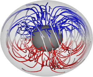
  $\phi$). Figure 1 shows this initial perturbation which subsequently evolves under gravity
  $\boldsymbol{g}=-g \hat {\boldsymbol {e}}_z$ and a uniform ambient magnetic field
  $\boldsymbol {B}=B \hat {\boldsymbol {e}}_z$. The initial temperature perturbation (2.1) gives rise to a velocity field
  $\boldsymbol {u}$, which in turn interacts with the mean field
  $\boldsymbol {B}$ to generate the induced magnetic field
  $\boldsymbol {b}$. The initial velocity
  $\boldsymbol {u}_0$ is zero, and since the magnetic field perturbation takes finite time to develop by induction, the initial induced field
  $\boldsymbol {b}_0$ is also zero. In the Boussinesq approximation, the following linearized MHD equations describe the evolution of
  $\boldsymbol {u}$,
  $\boldsymbol {b}$ and
  $\theta$:
 \begin{gather} \frac{\partial{\boldsymbol{u}}}{\partial{t}}={-}\frac{1}{\rho}\boldsymbol{\nabla} {p^*}+ \frac{1}{\mu \rho}(\boldsymbol{B} \boldsymbol{\cdot} \boldsymbol{\nabla} ) \boldsymbol{b} - \boldsymbol{g} \alpha\theta +\nu\nabla^2\boldsymbol{u}, \end{gather}
 \begin{gather}\frac{\partial{\boldsymbol{b}}}{\partial{t}} =(\boldsymbol{B} \boldsymbol{\cdot} \boldsymbol{\nabla} ) {\boldsymbol{u}} +\eta \nabla^2 \boldsymbol{b}, \end{gather}
 \begin{gather}\frac{\partial{\theta}}{\partial{t}}={-}\beta \boldsymbol{\hat{e}}_z \boldsymbol{\cdot} \boldsymbol{u}+ \kappa\nabla^2\theta, \end{gather}
 \begin{gather}\boldsymbol{\nabla} \boldsymbol{\cdot} \boldsymbol{u} = \boldsymbol{\nabla} \boldsymbol{\cdot} \boldsymbol{b}=0, \end{gather}
where  $\nu$ is the kinematic viscosity,
  $\kappa$ is the thermal diffusivity,
  $\eta$ is the magnetic diffusivity,
  $\mu$ is the magnetic permeability,
  $p^*=p+ \boldsymbol {b}^2/2\mu$ and
  $\beta =\partial T /\partial z$ is the mean axial temperature gradient. While the induction equation (2.3) is written in the limit of magnetic Reynolds number
  $Rm \ll 1$, it gives a close approximation for the field generation at length scales of
  $Rm \sim 1$ (Moffatt & Loper Reference Moffatt and Loper1994).

Figure 1. A density perturbation  $\rho ^\prime$ sits in a stably stratified fluid layer permeated by a poloidal magnetic field. In the present model,
  ${\boldsymbol B}$ is the uniform mean magnetic field acting in the
  $z$ direction.
2.1. Solutions of the initial value problem
As the initial temperature perturbation (2.1) gives rise to a purely poloidal flow, the instantaneous state of the flow is uniquely defined by (Davidson, Sreenivasan & Aspden Reference Davidson, Sreenivasan and Aspden2007)
 \begin{gather} \boldsymbol{u} = \boldsymbol{\nabla} \times [ (\psi/s) \hat{\boldsymbol{e}}_\phi ], \end{gather}
 \begin{gather}\nabla_*^2 \psi = \frac{\partial^2{\psi}}{\partial{z^2}}+s\frac{\partial}{\partial{s}} \left(\frac{1}{s}\frac{\partial{\psi}}{\partial{s}}\right) ={-}s \zeta_\phi, \end{gather}
where  $\psi$ is the Stokes streamfunction of the velocity and
  $\boldsymbol {\zeta }$ is the vorticity. In a similar way, the induced magnetic field is expressed as
 \begin{gather} \boldsymbol{b} = \boldsymbol{\nabla} \times [ (\xi/s) \hat{\boldsymbol{e}}_\phi ], \end{gather}
 \begin{gather}\nabla_*^2 \xi ={-}s \mu j_\phi, \end{gather}
where  $\xi$ is the Stokes streamfunction of the induced magnetic field and
  $\boldsymbol {j}$ is the electric current density.
Taking the  $\phi$ components of the curl of (2.2) and (2.3) and using (2.7), an equation for the evolution of
  $\psi$ follows:
 \begin{equation} \left[\left(\frac{\partial}{\partial{t}}-\nu\nabla_*^2\right) \left(\frac{\partial}{\partial{t}}-\eta\nabla_*^2\right)- V_M^2\frac{\partial^2{}}{\partial{z^2}}\right](\nabla_*^2\psi) =\left(\frac{\partial}{\partial{t}}-\eta\nabla^2\right) g\alpha s\frac{\partial{\theta}}{\partial{s}},\end{equation}
where  $V_M=B /\sqrt {\mu \rho }$ is the magnetic (Alfvén) wave velocity. A similar approach gives the equation for the evolution of
  $\xi$,
 \begin{equation} \left[\left(\frac{\partial}{\partial{t}}-\nu\nabla_*^2\right) \left(\frac{\partial}{\partial{t}}-\eta\nabla_*^2\right)- V_M^2\frac{\partial^2{}}{\partial{z^2}}\right](\nabla_*^2 \xi) = B g \alpha s \frac{\partial^2{\theta}}{\partial{z}\partial{s}}.\end{equation}
The Hankel–Fourier transforms
 \begin{gather} H_1 \{\psi(s,z)\} = \hat{\psi}(k_s,k_z) = \frac{1}{2{\rm \pi} ^2}\int_{0}^{\infty}\int_{0}^{\infty}\psi(s,z){J}_1(k_ss)\, \mbox{e}^{-\textrm{i}k_zz}\,\mbox{d}s\,\mbox{d}z, \end{gather}
 \begin{gather}H_0 \{\theta(s,z)\} = \hat{\theta}(k_s,k_z)= \frac{1}{2{\rm \pi} ^2}\int_{0}^{\infty}\int_{0}^{\infty}\theta(s,z){J}_0(k_ss) \,\mbox{e}^{-\textrm{i}k_zz}s\,\mbox{d}s\,\mbox{d}z, \end{gather}
where  ${J}_0$ and
  ${J}_1$ are the zeroth- and first-order Bessel functions of the first kind, are applied to (2.10),
 \begin{equation} \left[\left(\frac{\partial}{\partial{t}}+\nu k^2\right) \left(\frac{\partial}{\partial{t}}+\eta k^2\right)+ V_M^2k_z^2\right]\hat{\psi}=g\alpha\frac{k_s}{k^2}\frac{\partial{\hat{\theta}}} {\partial{t}} + g\alpha\eta k_s\hat{\theta},\end{equation}
where  $k^2=k_s^2+k_z^2$ and the following identities are used:
 \begin{equation} H_1 \{ f^\prime(s) \} ={-}k_s H_0 \{f(s) \}, \quad H_1 \{ s^{{-}1} \nabla_*^2 [sf(s)] \}={-}k^2 H_1 \{\,f(s) \}.\end{equation}
 Since the zeroth-order Hankel transform of  $u_z$ is given by
 \begin{align} \hat{u}_z & = \frac{1}{2{\rm \pi} ^2} \int_{0}^{\infty}\int_{0}^{\infty} \left(\frac1{s} \frac{\partial{{\psi}}}{\partial{s}}\right) {J}_0(k_s s)\, \mbox{e}^{-\textrm{i}k_z z} \, s \, \mbox{d}s \, \mbox{d}z, \end{align}
 \begin{align} &= \frac{1}{2{\rm \pi} ^2} \int_{0}^{\infty}\left[\int_{0}^{\infty} \left(\frac{\partial{{\psi}}}{\partial{s}}\right) {J}_0(k_s s) \, \mbox{d}s\right] \, \mbox{e}^{-\textrm{i}k_z z} \, \mbox{d}z, \end{align}
integration by parts using the identity  ${J}_0^\prime (s)= -{J}_1(s)$ gives
 \begin{equation} \hat{u}_z = \frac{k_s}{2{\rm \pi} ^2} \int_{0}^{\infty}\int_{0}^{\infty} \psi(s,z) {J}_1(k_s s) \, \mbox{e}^{-\textrm{i}k_z z} \, \mbox{d}s \, \mbox{d}z= k_s \hat{\psi}, \end{equation}
from (2.12). Consequently, the transform of (2.4),
 \begin{equation} \frac{\partial{\hat{\theta}}}{\partial{t}}={-}\beta k_s \hat{\psi} - \kappa k^2\hat{\theta},\end{equation}
is used in (2.14) to obtain the equation for the evolution of  $\hat {\psi }$,
 \begin{equation} \left[\left(\frac{\partial}{\partial{t}}+\nu k^2\right) \left(\frac{\partial}{\partial{t}}+\eta k^2\right) +V_M^2k_z^2+\frac{g\alpha \beta k_s^2}{k^2}\right] \left(\frac{\partial}{\partial{t}} +\kappa k^2\right)\hat{\psi}={-}g\alpha k_s^2(\eta-\kappa)\beta\hat{\psi}.\end{equation}
Seeking plane wave solution of the form  $\hat {\psi } \sim \mbox {e}^{\textrm {i}\lambda t}$ for (2.20), we obtain the relation
 \begin{equation} (\textrm{i}\lambda+\omega_\nu)(\textrm{i}\lambda+\omega_\eta)(\textrm{i}\lambda+\omega_\kappa)+ \omega_M^2(\textrm{i}\lambda+\omega_\kappa)+\omega_A^2(\textrm{i}\lambda+\omega_\eta)=0,\end{equation}
which consists of the fundamental frequencies  $\omega _M=V_M k_z$ (Alfvén wave),
  $\omega _A=\sqrt {g \alpha \beta } k_s/k$ (internal gravity wave),
  $\omega _\eta =\eta k^2$ (magnetic diffusion),
  $\omega _\nu =\nu k^2$ (viscous diffusion) and
  $\omega _\kappa =\kappa k^2$ (thermal diffusion). The subscripts
  $M$ and
  $A$ above represent waves of magnetic and Archimedean origin.
Equation (2.21) is of the form
 \begin{equation} \lambda^3+a_2\lambda^2+a_1\lambda+a_0=0,\end{equation}
where
 \begin{equation} \left.\begin{array}{c@{}} a_2 ={-}\textrm{i}(\omega_\eta+\omega_\kappa+\omega_\nu), \\ a_1 ={-}(\omega_A^2+\omega_\eta\omega_\kappa+ \omega_\eta\omega_\nu+\omega_\kappa\omega_\nu+\omega_M^2), \\ a_0 = \textrm{i}(\omega_A^2\omega_\eta+\omega_\kappa\omega_M^2+\omega_\eta\omega_\kappa\omega_\nu). \end{array}\right\} \end{equation}
To solve (2.22), we use the cubic formula (Dickson Reference Dickson1898; Dunham Reference Dunham1990). The solutions of (2.21) are then given by
 \begin{gather} \lambda_{1,2} ={\pm} \frac{\sqrt{3}}{12}\left(2^{2/3} Q+ \frac{2\sqrt[3]{2}P}{Q}\right)+\frac{\textrm{i}}{12} \left(4(\omega_\eta+\omega_\kappa+\omega_\nu)- 2^{2/3} Q+\frac{2\sqrt[3]{2}P}{Q}\right), \end{gather}
 \begin{gather}\lambda_3=\frac{\textrm{i}}{6}\left(2^{2/3}Q-\frac{2\sqrt[3]{2}P}{Q} +2(\omega_\eta+\omega_\kappa+\omega_\nu)\right), \end{gather}
where
 \begin{gather} P = 3 (\omega_A^2+\omega_M^2+\omega_\eta\omega_\kappa +(\omega_\eta+\omega_\kappa)\omega_\nu )- (\omega_\eta+\omega_\kappa+\omega_\nu )^2, \end{gather}
 \begin{gather}Q = \sqrt[3]{\sqrt{4P^3+R^2}+R}, \end{gather}
 \begin{align} R &= 9 \omega_A^2 (2\omega_\eta-\omega_\kappa-\omega_\nu) -9 \omega_M^2 (\omega_\eta - 2\omega_\kappa+\omega_\nu) \nonumber\\ & \quad + (\omega_\eta+\omega_\kappa-2\omega_\nu)(2\omega_\eta-\omega_\kappa-\omega_\nu) (\omega_\eta-2\omega_\kappa+\omega_\nu). \end{align}
The solutions (2.24a)–(2.24b) for the frequency may also be obtained by taking the transform of (2.11) for  $\xi$.
The general solutions for the transforms  $\hat {\psi }$ and
  $\hat {\xi }$ are then given by
 \begin{equation} [\hat{\psi},\hat{\xi}] = \sum_{m=1}^{3}[A_m,B_m]\,\mbox{e}^{\textrm{i} \lambda_m t}.\end{equation}
The coefficients  $A_m$ and
  $B_m$ are evaluated from the initial conditions for
  $\hat {\psi }$ and
  $\hat {\xi }$ and their time derivatives.
For a given time, the streamfunctions of the velocity (and induced magnetic field) may be recovered from (2.28) by the inverse Hankel–Fourier transform
 \begin{equation} f(s,z) = 4{\rm \pi} s\int_{0}^{\infty}\int_{0}^{\infty}\hat{f}(k_s,k_z) {J}_1(k_ss)\, \mbox{e}^{\textrm{i}k_zz} k_s\,\mbox{d}k_s\,\mbox{d}k_z.\end{equation}
2.1.1. Evaluation of spectral coefficients
From (2.28), the initial conditions for  $\hat {\psi }$ and its time derivatives are given by
 \begin{equation} {\rm i}^n\sum_{m=1}^{3}A_m\lambda_m^n= \left(\frac{\partial^n{\hat{\psi}}}{\partial{t^n}}\right)_{ 0}=a_{n+1}, \quad n=0,1,2.\end{equation}
where the subscript ‘0’ refers to the initial state. While the Hankel–Fourier transform of initial condition (2.1) gives  $\hat{\theta}_0$ (Abramowitz & Stegun Reference Abramowitz and Stegun1972), the conditions of zero initial velocity and induced magnetic field are necessary to evaluate the initial time derivatives of
  $\hat {\psi }$. Algebraic simplifications using the curl of (2.2) with (2.7) give the right-hand sides of (2.30) as follows:
 \begin{gather} a_1 = 0, \end{gather}
 \begin{gather}a_2 = \frac{ g \alpha k_s}{k^2} \hat{\theta}_0= \frac{g \alpha k_s\delta^3 \,\mbox{e}^{{-}k^2\delta^2/8}}{16\sqrt{2}{\rm \pi} ^{3/2}k^2}, \end{gather}
 \begin{gather}a_3 ={-} g \alpha k_s (\nu+\kappa)\hat{\theta}_0={-} \frac{g \alpha k_s(\nu+\kappa)\delta^3 \,\mbox{e}^{- k^2\delta^2/8}}{16\sqrt{2}{\rm \pi} ^{3/2}}. \end{gather}
Equations (2.31)–(2.33) give the coefficients of the velocity transform,
 \begin{equation} A_1\!=\!{-}\frac{a_3-{\rm i}a_2(\lambda_2+\lambda_3)}{(\lambda_1-\lambda_2)(\lambda_1-\lambda_3)}, \quad A_2 \!=\!{-}\frac{a_3-{\rm i}a_2(\lambda_1+\lambda_3)}{(\lambda_2-\lambda_3)(\lambda_2-\lambda_1)}, \quad A_3 \!=\!{-}\frac{a_3-{\rm i}a_2(\lambda_1+\lambda_2)}{(\lambda_3-\lambda_1)(\lambda_3-\lambda_2)}. \end{equation}
From (2.28), the initial conditions for  $\hat {\xi }$ and its time derivatives are given by
 \begin{equation} {\rm i}^n\sum_{m=1}^{3}B_m\lambda_m^n= \left(\frac{\partial^n{\hat{\xi}}}{\partial{t^n}}\right)_{ 0}=b_{n+1}, \quad n=0,1,2.\end{equation}
The right-hand sides of (2.35) are obtained as follows:
 \begin{gather} b_1 = b_2 = 0, \end{gather}
 \begin{gather}b_3 = \textrm{i} \frac{g \alpha B k_s k_z \delta^3 \,\mbox{e}^{- k^2\delta^2/8}}{16\sqrt{2}{\rm \pi} ^{3/2} k^2}. \end{gather}
The coefficients of the magnetic field transform are then given by
 \begin{equation} B_1 ={-}\frac{b_3-{\rm i}b_2(\lambda_2\!+\!\lambda_3)}{(\lambda_1-\lambda_2)(\lambda_1\!-\!\lambda_3)}, \quad B_2 ={-}\frac{b_3-{\rm i}b_2(\lambda_1\!+\!\lambda_3)}{(\lambda_2-\lambda_3)(\lambda_2\!-\!\lambda_1)}, \quad B_3 ={-}\frac{b_3-{\rm i}b_2(\lambda_1\!+\!\lambda_2)}{(\lambda_3-\lambda_1)(\lambda_3 \!-\!\lambda_2)}.\end{equation}
In the sections below, we present approximate analytical solutions in the limit of zero viscous and thermal diffusion that describe the long-time evolution of magnetically damped waves initiated by a density perturbation in a stably stratified fluid. Two limits are analysed, that of strong stratification and that of strong magnetic field. The theory is then compared with computations of the general solution using  $\nu , \kappa \ll \eta$.
2.2. The case of strong stratification
In the limit of zero viscous and thermal diffusion ( $\nu =\kappa =0$), the orders of magnitude of the fundamental frequencies for this case are given by
  $\omega _A \gg \omega _M \gg \omega _\eta$. Since the diffusion of disturbances along the magnetic field lines does not result in a reduction in
  $\omega _A$, a diffusion-dominated regime where
  $\omega _\eta \gg \omega _A$ is not anticipated.
When terms up to second order in  $(\omega _M/\omega _A)$ are considered, the frequencies (2.24a)–(2.24b) are approximated by (Appendix B)
 \begin{gather} \lambda_{1,2} \approx{\pm} \omega_A \left(1+\frac{{\omega_M}^2}{{2\omega_A}^2} \right) +\textrm{i} \frac{{\omega_M}^2 \omega_\eta}{2{\omega_A}^2} ={\pm} R_1 +\textrm{i} I_{11}, \end{gather}
 \begin{gather}\lambda_3 \approx \textrm{i} \omega_\eta \left(1-\frac{{\omega_M}^2}{{\omega_A}^2}\right) =\textrm{i} I_{12}. \end{gather}
The spectral coefficients in (2.34a–c) then take the approximate form
 \begin{equation} A_1 \approx \textrm{i}\frac{a_2}{2\omega_A}, \quad A_2 \approx{-}\textrm{i} \frac{a_2}{2\omega_A}, \quad A_3 \approx\frac{a_2}{2\omega_A} \left(\frac{2 \omega_M^2 \omega_\eta}{\omega_A^3}\right).\end{equation}
where  $a_2$ is given by (2.32). The transform of the velocity streamfunction is then,
 \begin{equation} \hat{\psi}\approx A_1 \mathrm{e}^{-\textrm{i} R_1 t - I_{11} t} + A_2 \mathrm{e}^{\textrm{i} R_1 t - I_{11} t}, \end{equation}
since  $A_3 \to 0$. Further simplification using (2.40a–c) yields
 \begin{equation} \hat{\psi}\approx \textrm{i} \frac{a_2}{2\omega_A}( \mbox{e}^{-\textrm{i} R_1 t } - \mbox{e}^{\textrm{i} R_1 t })\, \mbox{e}^{- I_{11}t} \approx \frac{a_2}{\omega_A} \, \mbox{e}^{{-}I_{11}t} \sin{(R_1t)}.\end{equation}
A similar approach gives the spectral coefficients in (2.38a–c) in the approximate form
 \begin{equation} B_1 \approx \frac{b_3}{2\omega_A^2}\left({-}1+ \textrm{i}\frac{\omega_\eta}{\omega_A}\right),\quad B_2 \approx \frac{b_3}{2\omega_A^2}\left({-}1-\textrm{i}\frac{\omega_\eta}{\omega_A}\right),\quad B_3 \approx \frac{b_3}{\omega_A^2},\end{equation}
where  $b_3$ is given by (2.37). The transform of the induced field streamfunction is then,
 \begin{equation} \hat{\xi} \approx B_1 \, \mathrm{e}^{-\textrm{i} R_1 t - I_{11} t} + B_2 \,\mathrm{e}^{\textrm{i} R_1 t - I_{11} t} + B_3 \, \mathrm{e}^{{-}I_{12}t}. \end{equation}
Further simplification using (2.43a–c) yields
 \begin{equation} \hat{\xi} \approx \frac{b_3}{\omega_A^2}\left[-\cos{(R_1t)} \, \mbox{e}^{- I_{11}t} +\frac{\omega_\eta}{\omega_A}\sin{(R_1t)} \, \mbox{e}^{- I_{11}t} + \mbox{e}^{- I_{12}t}\right]. \end{equation}
2.2.1. Long-time evolution of kinetic energy
Since  $\vert {\hat {u}}\vert ^2=k^2\vert {\hat {\psi }}\vert ^2$, (2.42) gives
 \begin{equation} \vert {\hat{u}}\vert ^2\approx\frac{\vert {a_2}\vert ^2k^2}{\omega_A^2}\, \textrm{e}^{{-}2I_{11}t}\sin^2{(R_1t)}.\end{equation}
Using (2.31) and the expressions for the frequencies  $\omega _A, \omega _M$ and
  $\omega _\eta$ in (2.42), we obtain
 \begin{equation} \vert {\hat{u}}\vert ^2 \approx\exp{\left(- \frac{k^2\delta^2}{4}\right)} \left(\frac{g\alpha \delta^6}{512{\rm \pi} ^{3}\beta}\right) \exp{\left(-\frac{V_M^2\eta k^4k_z^2}{g\alpha\beta k_s^2}t\right)} \sin^2{\left(\sqrt{g\alpha \beta}\frac{k_s}{k}t\right)}.\end{equation}
The initial temperature perturbation (2.1) releases energy into the poloidal flow on the time scale
 \begin{equation} t_A=\frac1{\sqrt{g \alpha \beta}} \frac{k_0}{k_{s0}}, \end{equation}
where  $k_0=\sqrt {6}/\delta$ is the initial wavenumber of the disturbance (Appendix C) and
  $k_{s0}=k_0/\sqrt {2}$. This flow subsequently undergoes magnetic damping on the time scale
 \begin{equation} t_1=\frac{g \alpha \beta}{V_M^2 \eta k_0^4}, \end{equation}
as  $k_{z0}=k_{s0}$. Since the kinetic energy is given by Parseval's theorem as (Sreenivasan & Narasimhan Reference Sreenivasan and Narasimhan2017)
 \begin{equation} E_{k} = 16 {\rm \pi}^4 \int_{0}^{\infty} \int_{0}^{\infty} |\hat{u}|^2 k_s \, \mbox{d}k_s \, \mbox{d}k_z,\end{equation}
for  $t \gtrsim t_1$, the kinetic energy is expanded as
 \begin{equation} E_{k} \approx 16{\rm \pi} ^4\int_{0}^{\infty}\int_{0}^{\infty} \left(\frac{g\alpha \delta^6}{512{\rm \pi} ^{3}\beta}\right) \exp{\left( - \frac{k^2\delta^2}{4}\right)}\exp{\left(-\frac{V_M^2\eta k^4k_z^2} {g\alpha\beta k_s^2}t\right)} k_s\, \mathrm{d}k_s\,\mathrm{d}k_z.\end{equation}
Using the substitutions  $k_z=k\cos \vartheta$ and
  $k_s=k \sin \vartheta$ (Sreenivasan & Narasimhan Reference Sreenivasan and Narasimhan2017),
 \begin{equation} E_{k} \approx\frac{{\rm \pi} g\alpha \delta^6 }{32\beta} \int_{0}^{\infty}\int_{0}^{{\rm \pi} /2}k^2\exp{\left(- \frac{k^2\delta^2}{4}\right)} \exp{\left(-\frac{V_M^2\eta k^4\cot^2\vartheta}{g\alpha\beta}t\right)} \sin\vartheta\,\mbox{d}\vartheta\,\mbox{d}k.\end{equation}
Letting  $x=\cot ^2\vartheta$, (2.52) may be rewritten as
 \begin{equation} E_k \approx \frac{{\rm \pi} g\alpha \delta^6 }{64\beta} \int_{0}^{\infty}\int_{0}^{\infty} k^2 \exp \left( - \frac{k^2\delta^2}{4}\right) \exp \left( -\frac{V_M^2\eta k^4 x}{g\alpha\beta}t \right) x^{{-}1/2}(1+x)^{{-}3/2}\,\mbox{d}x\,\mbox{d}k.\end{equation}
Using the relation (13.2.5 in Abramowitz & Stegun Reference Abramowitz and Stegun1972)
 \begin{equation} \varGamma(\textit{a}){U}(a,b,z)=\int_{0}^{\infty} \,\mbox{e}^{{-}z \tau} \tau^{a-1}(1+\tau)^{b-a-1}\,\mbox{d}\tau, \end{equation}
where  $\varGamma$ is the gamma function,
  ${U}$ is the confluent hypergeometric function,
  $a=1/2$,
  $b=0$ and
  $z=V_M^2 \eta k^4 t/g \alpha \beta$, (2.53) simplifies to
 \begin{equation} E_k\approx\frac{{\rm \pi} g\alpha \delta^6 }{64\beta} \int_{0}^{\infty} k^2 \exp{\left(-\frac{k^2\delta^2}{4} \right)} \varGamma\left(\frac{1}{2}\right) {U}\left(\frac1{2},0, \frac{V_M^2\eta k^4}{g\alpha\beta} t\right)\,\mbox{d}k.\end{equation}
Since the asymptotic value of  ${U}$ as
  $z\to \infty$ is given by (13.1.8 in Abramowitz & Stegun Reference Abramowitz and Stegun1972)
 \begin{equation} {U}(a,b,z)\sim z^{{-}a} [1 + O (\vert {z}\vert ^{{-}1} ) ],\end{equation}
for  $t \gg t_1$, (2.55) further reduces to
 \begin{equation} E_k \approx \frac{{\rm \pi} ^{3/2} g\alpha \delta^6 }{64\beta} \int_{0}^{\infty} \exp \left( -\frac{k^2\delta^2}{4} \right) \left(\frac{t}{k_0^4 t_1} \right)^{{-}1/2}\, \mbox{d}k.\end{equation}
Finally, integration over the wavenumber  $k$ yields
 \begin{equation} E_k\approx\frac{3 {\rm \pi}^{2} g\alpha \delta^3}{32 \beta}\left(\frac{t}{t_1}\right)^{{-}1/2}, \end{equation}
by using the relation  $k_0 \delta =\sqrt {6}$ for the initial perturbation (2.1). Thus, for
  $t \gg t_1$, the kinetic energy decays as
  $(t/t_1)^{-1/2}$.
2.2.2. Long-time evolution of magnetic energy
Since  $|\hat {b}|^2=k^2|\hat {\xi }|^2$, (2.44) gives
 \begin{align} |\hat{b}|^2&\approx k^2 \frac{\vert {b_3}\vert ^2}{\omega_A^4} \left[\mbox{e}^{{-}2I_{12}t}-2\mbox{e}^{-(I_{11}+I_{12})t} \cos{(R_1t)}+ \mbox{e}^{{-}2I_{11}t} \cos^2{(R_1t)}\vphantom{\frac{\omega_\eta^2}{\omega_A^2}}\right.\nonumber\\ &\quad + 2 \, \mbox{e}^{{-}I_{12}t} \frac{\omega_\eta}{\omega_A} \mbox{e}^{{-}I_{11}t} \sin{(R_1t)} - 2 \, \mbox{e}^{{-}2I_{11}t} \frac{\omega_\eta}{\omega_A}\cos{(R_1t)}\sin{(R_1t)}\nonumber\\ &\quad + \left.\mbox{e}^{{-}2I_{11}t}\frac{\omega_\eta^2}{\omega_A^2}\sin^2{(R_1t)}\right]. \end{align}
Noting that the inequality  ${R_1}^{-1} \ll {I_{12}}^{-1} \ll {I_{11}}^{-1}$ is satisfied by the time scales, the long-time evolution of
  $|\hat {b}|^2$ is determined by the term that decays slowest,
 \begin{equation} |\hat{b}|^2 \approx k^2 \frac{\vert {b_3}\vert ^2}{\omega_A^4}\, \mbox{e}^{{-}2I_{11}t}.\end{equation}
Since the magnetic energy is given by Parseval's theorem as
 \begin{equation} E_m = \frac{16 {\rm \pi}^4}{\mu \rho} \int_{0}^{\infty} \int_{0}^{\infty} {\vert {\hat{b}}\vert }^2 k_s \, \mbox{d}k_s \, \mbox{d}k_z, \end{equation}
using (2.37) and the expressions for the frequencies  $\omega _A, \omega _M$ and
  $\omega _\eta$ in (2.60), we obtain the magnetic energy for times
  $t \gtrsim t_1$,
 \begin{equation} E_m \approx \frac{{\rm \pi} \delta^6 V_M^2}{32 \beta^2} \int_{0}^{\infty}\int_{0}^{\infty} \frac{k^2 k_z^2}{k_s^2} \exp{\left(- \frac{k^2\delta^2}{4}\right)} \exp{\left(-\frac{V_M^2\eta k^4k_z^2} {g\alpha\beta k_s^2}t\right)} k_s\,\mbox{d}k_s\,\mbox{d}k_z. \end{equation}
Using the substitutions  $k_z=k\cos \vartheta$ and
  $k_s=k\sin \vartheta$,
 \begin{equation} E_m \approx \frac{{\rm \pi} \delta^6 V_M^2}{32\beta^2} \int_{0}^{\infty}\int_{0}^{{\rm \pi} /2} k^4\exp{\left(- \frac{k^2\delta^2}{4} - \frac{V_M^2\eta k^4\cot^2\vartheta}{g\alpha\beta}t\right)} \cot^2\vartheta \sin\vartheta \, \mbox{d}\vartheta \, \mbox{d}k. \end{equation}
The integral in (2.63), of the form
 \begin{equation} I_A=\int_{0}^{\infty} k^4\exp ({-}a k^2-b k^4) \ \textrm{d} k, \end{equation}
where  $a=\delta ^2/2$ and
  $b=({V^2_M \eta \cot ^2 \vartheta }/{g \alpha \beta }) t$, has the following solution (see 3.469, Gradshteyn & Ryzhik Reference Gradshteyn and Ryzhik2007):
 \begin{equation} I_A = \frac{\sqrt{a} \exp ( a^2/8b )}{32 b^{5/2}} \left[(a^2 + 2 b) K_{1/4}\left(\frac{a^2}{8b}\right)- a^2 K_{3/4}\left(\frac{a^2}{8b}\right)\right], \end{equation}
where  $K_{n}(x)$ is the modified Bessel function of the second kind. In the limit
  $b\rightarrow \infty$ (
 $t \gg t_1$),
  $I_A$ is approximated by (Sreenivasan & Narasimhan Reference Sreenivasan and Narasimhan2017)
 \begin{equation} I_A\approx \frac{\varGamma(1/4)b^{{-}5/4}}{16}+O(b^{{-}7/4}). \end{equation}
Therefore, (2.63) simplifies to
 \begin{equation} E_m\approx \frac{36 \sqrt{6} {\rm \pi}\delta V_M^2}{512\beta^2} I_\vartheta \varGamma{\left(\frac{1}{4}\right)} \left(\frac{t}{t_1}\right)^{{-}5/4},\end{equation}
where the integral  $I_\vartheta$ is related to the beta function by (3.621, Gradshteyn & Ryzhik Reference Gradshteyn and Ryzhik2007)
 \begin{align} I_\vartheta &= \int_{0}^{{\rm \pi} /2} (\cot^2\vartheta)^{{-}5/4} \cot^2\vartheta \sin\vartheta\, \mbox{d}\vartheta = \frac{1}{2} \mathtt{B}(5/4,1/4), \end{align}
 \begin{align} &\approx 1.854. \end{align}
Thus, for  $t \gg t_1$, the magnetic energy decays as
  $(t/t_1)^{-5/4}$.
2.3. The case of strong magnetic field
In the limit of zero viscous and thermal diffusion ( $\nu =\kappa =0$), the orders of magnitude of the fundamental frequencies for this case are given by
  $\omega _M \gg \omega _A \gg \omega _\eta$. When terms up to second order in
  $(\omega _A/\omega _M)$ are considered, the frequencies (2.24a)–(2.24b) are approximated by
 \begin{gather} \lambda_{1,2} \approx{\pm} \omega_M \left(1+\frac{{\omega_A}^2}{{2\omega_M}^2} \right) + \textrm{i} \frac{\omega_\eta}{2} \left(1- \frac{{\omega_A}^2}{{\omega_M}^2} \right) ={\pm} R_{2} +\textrm{i} I_{21}, \end{gather}
 \begin{gather}\lambda_3 \approx \textrm{i} \frac{{\omega_A}^2\omega_\eta}{{\omega_M}^2} =\textrm{i} I_{22}. \end{gather}
The spectral coefficients in (2.34a–c) then take the approximate form
 \begin{equation} A_1 \approx \frac{a_2}{2\omega_M}\left(-\frac{\omega_\eta}{\omega_M} + \textrm{i} \right), \quad A_2 \approx \frac{a_2}{2\omega_M} \left(-\frac{\omega_\eta}{\omega_M} -\textrm{i} \right), \quad A_3 \approx\frac{a_2}{2\omega_M} \left( \frac{2 \omega_\eta}{\omega_M} \right),\end{equation}
where  $a_2$ is given by (2.32). The transform of the velocity streamfunction is then,
 \begin{equation} \hat{\psi}\approx A_1 \, \mbox{e}^{(-\textrm{i}R_2-I_{21}) t}+ A_2 \, \mbox{e}^{(\textrm{i}R_2- I_{21})t} + A_3 \, \mbox{e}^{{-}I_{22}t}.\end{equation}
Further simplification using (2.71a–c) yields
 \begin{equation} \hat{\psi}\approx\frac{a_2}{\omega_M}\left[ \left(-\frac{\omega_\eta}{\omega_M} \right)\, \mbox{e}^{{-}I_{21} t} \cos(R_2 t ) + \mbox{e}^{{-}I_{21} t} \sin(R_2 t ) + \left( \frac{ \omega_\eta}{\omega_M} \right)\, \mbox{e}^{{-}I_{22} t}\right]. \end{equation}
A similar approach gives the spectral coefficients in (2.38a–c) in the approximate form
 \begin{equation} B_1 \approx \frac{b_3}{2 \omega_M^2} \left({-}1 -\textrm{i} \frac{\omega_\eta}{2 \omega_M}\right),\quad B_2 \approx \frac{b_3}{2 \omega_M^2} \left({-}1 +\textrm{i} \frac{\omega_\eta}{2 \omega_M}\right),\quad B_3 \approx \frac{b_3}{\omega_M^2}, \end{equation}
where  $b_3$ is given by (2.37). The transform of the induced field streamfunction is then,
 \begin{align} \hat{\xi} &\approx B_1 \, \mbox{e}^{(-\textrm{i}R_2-I_{21}) t} +B_2 \, \mbox{e}^{(\textrm{i}R_2- I_{21})t} + B_3 \, \mbox{e}^{{-}I_{22}t}, \end{align}
 \begin{align} & \approx \frac{b_3}{\omega_M^2} \left[-\mbox{e}^{{-}I_{21} t} \cos(R_2 t ) - \frac{ \omega_\eta}{2 \omega_M} \mbox{e}^{{-}I_{21} t} \sin(R_2 t ) + \mbox{e}^{{-}I_{22} t}\right]. \end{align}
Since  $\vert {\hat {u}}\vert ^2=k^2\vert {\hat {\psi }}\vert ^2$ and
  ${\vert {\hat {b}}\vert }^2 = k^2 {\vert {\hat {\xi }}\vert }^2$, (2.73) and (2.76) give
 \begin{align} \vert {\hat{u}}\vert ^2 & \approx\frac{\vert {a_2}\vert ^2k^2}{\omega_M^2} \left[\left(\frac{\omega_\eta}{\omega_M}\right)^2 \, \mbox{e}^{{-}2I_{22}t}- 2 \, \mbox{e}^{-(I_{21}+I_{22})t} \left(\frac{\omega_\eta}{\omega_M}\right)^2 \cos{(R_2 t)}\right.\nonumber\\ &\quad + \mbox{e}^{{-}2I_{21}t} \left(\frac{\omega_\eta}{\omega_M}\right)^2 \cos^2{(R_2t)} +2 \, \mbox{e}^{-(I_{21}+I_{22}) t}\left(\frac{\omega_\eta}{\omega_M}\right)\sin{(R_{2}t)}\nonumber\\ &\quad \left.-2 \, \mbox{e}^{{-}2I_{21}t} \left(\frac{\omega_\eta}{\omega_M}\right)\cos{(R_2t)}\sin{(R_2t)}+ \mbox{e}^{{-}2I_{21}t}\sin^2{(R_2t)}\right], \end{align}
 \begin{align} \vert {\hat{b}}\vert ^2& \approx\frac{\vert {b_3}\vert ^2k^2}{\omega_M^4} \left[\mbox{e}^{{-}2I_{22}t}-2 \, \mbox{e}^{-(I_{21}+I_{22})t}\cos{(R_2 t)}+ \mbox{e}^{{-}2I_{21}t} \cos^2{(R_2t)} \vphantom{\frac{\omega_\eta^2}{4\omega_M^2}}\right.\nonumber\\ & \quad -\frac{\omega_\eta}{\omega_M} \mbox{e}^{-(I_{21}+I_{22}) t}\sin{(R_2t)} +\frac{\omega_\eta}{\omega_M} \mbox{e}^{{-}2I_{21}t}\cos{(R_2t)}\sin{(R_2t)}\nonumber\\ &\quad \left.+\frac{\omega_\eta^2}{4\omega_M^2}\, \mbox{e}^{{-}2I_{21}t} \sin^2{(R_2t)}\right]. \end{align}
We note that energy is released into the poloidal flow and field on the time scale
 \begin{equation} t_M= (V_M k_{z0})^{{-}1}. \end{equation}
Since the inequality  ${R_2}^{-1} \ll {I_{21}}^{-1} \ll {I_{22}}^{-1}$ is satisfied by the time scales, for
  ${I_{21}}^{-1} < t < {I_{22}}^{-1}$,
 \begin{equation} \vert {\hat{u}}\vert ^2 \approx \frac{\vert {a_2}\vert ^2k^2}{\omega_M^2}\, \mbox{e}^{{-}2I_{21} t}, \quad \vert {\hat{b}}\vert ^2 \approx \frac{\vert {b_3}\vert ^2k^2}{\omega_M^4}\, \mbox{e}^{{-}2I_{21}t}, \end{equation}
which gives
 \begin{equation} \vert {\hat{u}}\vert ^2= \frac1{\mu \rho}\vert {\hat{b}}\vert ^2 \approx \frac{g^2 \alpha^2 \delta^6}{512 {\rm \pi}^3 V_M^2} \left(\frac{k_s^2}{k_z^2 k^2}\right) \exp{\left[- k^2 \left( \frac{\delta^2}{4} + \eta t \right) \right]}. \end{equation}
The kinetic and magnetic energies evolve in equipartition in this Alfvénic regime.
The long-time decay of classical MHD turbulence would be diffusion dominated as the Alfvén wave frequency progressively decreases and falls below the diffusion frequency (Lehnert Reference Lehnert1955; Moffatt Reference Moffatt1967; Sreenivasan & Narasimhan Reference Sreenivasan and Narasimhan2017). However, as we see below, stable stratification limits the dominance of magnetic diffusion as the frequency of internal gravity waves remains large relative to that of diffusion.
2.3.1. Long-time evolution of energy
From the relative magnitudes of the time scales given by  ${R_2}^{-1} \ll {I_{21}}^{-1} \ll {I_{22}}^{-1}$, the long-time evolution of
  $\vert {\hat {u}}\vert ^2$ is described by the term that decays slowest in (2.77),
 \begin{equation} \vert {\hat{u}}\vert ^2 \approx\frac{\vert {a_2}\vert ^2k^2}{\omega_M^2} \left(\frac{\omega_\eta}{\omega_M}\right)^2 \, \mbox{e}^{{-}2I_{22}t}. \end{equation}
In the strong-field limit of Lundquist number  $S \to \infty$,
  $\omega _\eta /\omega _M \to 0$, so a finite kinetic energy via (2.82) necessitates a progressive decrease of
  $\omega _M$ until the two frequencies are of the same order. In classical MHD turbulence at
  $S \gg 1$, the onset of diffusive decay occurs when
  $\omega _M \sim \omega _\eta$, at time
  $t \sim S^{1/2} t_\eta$ (Moffatt Reference Moffatt1967). In a stratified MHD layer, however, the decrease of
  $\omega _M$ would lead to the regime
  $\omega _A \gg \omega _M \gg \omega _\eta$, in which the evolution of kinetic energy is described by (2.58) (see § 2.2.1). We shall return to this point in § 2.4.
The long-time evolution of  $\vert {\hat {b}}\vert ^2$ is determined by the term that decays slowest in (2.78),
 \begin{equation} \vert {\hat{b}}\vert ^2\approx\frac{\vert {b_3}\vert ^2k^2}{\omega_M^4} \,\mbox{e}^{{-}2I_{22}t}, \end{equation}
which remains finite for  $S \to \infty$. Using (2.37) and the expressions for the frequencies
  $\omega _A, \omega _M$ and
  $\omega _\eta$ in (2.83), we obtain
 \begin{equation} \frac1{\mu \rho} \vert {\hat{b}}\vert ^2 \approx \frac{g^2\alpha^2\delta^6}{512 {\rm \pi}^3 V_M^2} \left(\frac{k_s^2}{k_z^2 k^2}\right) \exp{\left(-\frac{k^2 \delta^2}{4}\right)} \exp{\left(-\frac{2g\alpha\beta \eta k_s^2}{V_M^2k_z^2}t\right)},\end{equation}
which indicates that the magnetic energy undergoes damping on the time scale
 \begin{equation} t_2 = \frac{V_M^2}{g \alpha \beta \eta}. \end{equation}
The transformation to polar coordinates  $(k,\vartheta )$ gives the magnetic energy for times
  $t \gtrsim t_2$,
 \begin{equation} E_m\approx\frac{{\rm \pi} g^2\alpha^2\delta^6}{32V_M^2}\int_{0}^{\infty}\int_{0}^{{\rm \pi} /2} \exp{\left(-\frac{k^2 \delta^2}{4}\right)} \exp{\left(-\frac{2t}{t_2} \tan^2\vartheta \right)} \frac{\sin^3\vartheta}{\cos^2\vartheta} \,\mbox{d}\vartheta\,\mbox{d}k.\end{equation}
Letting  $x = \tan ^2 \vartheta$, and using the identity (2.54) with
  $a=2$,
  $b=3/2$ and
  $z=2t/t_2$,
 \begin{equation} E_m\approx \frac{{\rm \pi} g^2\alpha^2\delta^6}{64V_M^2} \int_{0}^{\infty} \exp{\left(-\frac{k^2 \delta^2}{4}\right)} \varGamma(2) {U}\left(2,\frac{3}{2},\frac{2t}{t_2}\right)\,\mbox{d}k.\end{equation}
The asymptotic value of  ${U}$ as
  $z \to \infty$ (
 $t \gg t_2$) is obtained from (2.56). Integration over the wavenumber
  $k$ in turn yields
 \begin{equation} E_m \approx \frac{{\rm \pi} ^{3/2} g^2\alpha^2\delta^5}{256 V_M^2} \left(\frac{t}{t_2}\right)^{{-}2}.\end{equation}
For  $t \gg t_2$, the magnetic energy of the disturbances decays as
  $(t/t_2)^{-2}$.
2.3.2. Wave transition time scales
As the waves generated in the regime  $\omega _M \gg \omega _A$ undergo progressive diffusion,
  $\omega _M$ decreases with time, and eventually, Alfvénic waves would be transformed into waves whose frequency is buoyancy dominant. The kinetic energy undergoes this transition at time
  $t \lesssim t_2$ (§ 2.3.1). The time scale for the magnetic energy transition is obtained from (2.88) and (2.67) as follows:
 \begin{equation} 0.02175 \frac{g^2\alpha^2\delta^5}{V_M^2} \left(\frac{t}{t_2}\right)^{{-}2} \approx 3.637 \frac{\delta V_M^2}{\beta^2} \left(\frac{t}{t_1}\right)^{{-}5/4}, \end{equation}
which gives
 \begin{equation} t\approx 0.43 M^{4/3} t_2, \quad M=\frac{V_M}{\delta \sqrt{g \alpha \beta}}, \end{equation}
where  $M$ measures the initial ratio of the Alfvén wave frequency to the internal gravity wave frequency. The magnetic energy decays as
  $t^{-2}$ in the regime of strong field until
  $t \sim M^{4/3} t_2$, and subsequently crosses over to the regime of strong stratification wherein it decays as
  $t^{-5/4}$.
2.4. Computations of the long-time evolution of an isolated disturbance
The general solution of the initial value problem, given by (2.28), is computed. The values of the transforms  $\hat {\psi }$ and
  $\hat {\xi }$ in
  $(k_s,k_z)$ space and their respective energies are calculated at several time points. The kinetic and magnetic energies are calculated from the exact velocity and magnetic field transforms in (2.28) by Parseval's theorem (see e.g. (2.50) and (2.61)), where the upper limits of the integrals are the truncation values of
  $k_s$ and
  $k_z$. (The truncation value of the wavenumbers is set to
  $3/\delta$.) The computed energies are then compared with their asymptotic values derived from the leading-order solutions of the transforms in the limit of zero viscous and thermal diffusivities (
 $\nu =\kappa =0$).
In the calculations, both  $\nu$ and
  $\kappa$ are taken to be small relative to magnetic diffusivity
  $\eta$. The magnetic Prandtl number,
  $Pm=\nu /\eta = 10^{-8}$ and the Roberts number
  $q=\kappa /\eta =10^{-7}$. The strong-field regime is studied using the parameters
  $S=V_M \delta /\eta =10^4$ and
  $M=V_M/\delta \sqrt {g \alpha \beta } =316$. With small but finite magnetic diffusion, the frequencies in general change with time because the wavenumbers on which they depend are time varying. To compute the frequencies, the mean values of the wavenumbers are first calculated through ratios of
  $L^2$ norms; e.g.
 \begin{equation} \bar{k}_z = \frac{\|k_z \hat{\psi} k\|}{\| \hat{\psi} k\|}, \quad \bar{k} = \frac{\| \hat{\psi} k^2\|}{\| \hat{\psi} k \|},\end{equation}
which are based on the velocity field. As we anticipate that the frequencies based on the induced magnetic field would evolve differently, the mean wavenumbers based on  $\hat {\xi }$ are also evaluated following the definitions in (2.91a,b).
In figure 2(a,b), the imaginary parts of the frequencies  $\lambda _1$ and
  $\lambda _3$ in (2.24a,b) are compared with the respective frequency approximations. The parameters are those for the case of strong field,
  $S=10^4$ and
  $M=316$. The frequencies are calculated using the mean wavenumbers based on the induced magnetic field, so that a transition to the regime of dominant stratification may be observed, as predicted by theory. Here,
  $\textrm {Im}(\lambda _1)$ agrees well with
  $\omega _\eta /2 (1 - \omega _A^2/\omega _M^2 )$ (see (2.70a)) until time
  $t \sim 10^3 t_2$, and with
  $\omega _M^2 \omega _\eta /\omega _A^2$ (see (2.39a)) for
  $t > 10^3 t_2$. As the time scale for the strong-field regime to cross over to the regime of strong stratification is
  $t \approx 928 t_2$ (from (2.90a,b), shown by the vertical dashed-dotted lines in figure 2), it is apparent that the frequencies obey this transition. Figure 3(a) compares the computed kinetic and magnetic energies with their asymptotic solutions for the case of strong magnetic field. The energies are normalized by the reference magnetic energy, given by (2.88). In the early phase that lasts until
  $t \sim t_2$, the energies evolve in approximate equipartition, in line with (2.81). The
  $\sim t^{-1/2}$ decay of
  $E_k$ and
  $E_m$ with stratification is much slower than that in the absence of stratification, where the energies would have decayed as
  $\sim (t/t_\eta )^{-5/2}$ (Moffatt Reference Moffatt1967). The contours of the streamfunction in this early phase (figure 4), obtained from the inverse Hankel–Fourier transform, reveal the predominantly Alfvénic character of the wave since the front propagates as
  $z/\delta \approx t/t_M$. (Here,
  $t_M$ is the Alfvén wave travel time.) The evolution of energies is consistent with the time variation of the fundamental frequencies
  $\omega _M$,
  $\omega _A$ and
  $\omega _\eta$ calculated using the mean wavenumbers. For
  $t > t_2$,
  $E_k$ continues on its
  $\sim t^{-1/2}$ decay as the frequencies calculated based on the velocity cross-over to the regime of strong stratification, where
  $\omega _A > \omega _M$ (figure 3c). The triangles in figure 3(a) represent the asymptotic kinetic energy for strong stratification, given by (2.58). For a larger Lundquist number
  $S=10^5$, the transition to the regime of dominant
  $\omega _A$ occurs at
  $t < t_2$ (figure 3d), so it is evident that the evolution of the velocity as damped Alfvén waves is confined to this early period. The induced magnetic field, on the other hand, evolves as Alfvén waves until
  $t \approx 0.43 M^{4/3} t_2$ (figure 3b), which explains why
  $E_m$ follows the
  $t^{-2}$ decay law given by (2.88) for the period
  $t_2 < t < 0.43 M^{4/3} t_2$. For
  $t \gg M^{4/3} t_2$,
  $\omega _A \gg \omega _M$, which explains why
  $E_m$ follows the
  $t^{-5/4}$ law given by (2.67).
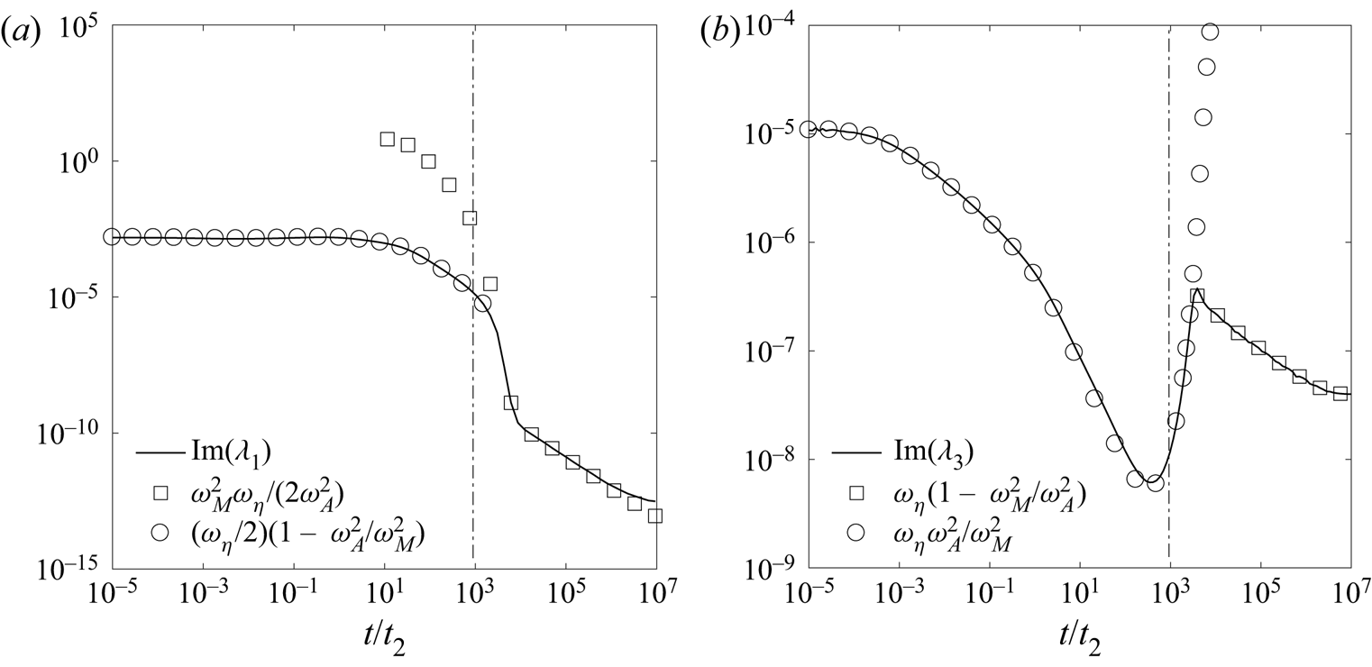
Figure 2. A comparison of the computed imaginary parts of the frequencies  $\lambda _1$ and
  $\lambda _3$ (solid lines) with their approximations (symbols) for the case of strong magnetic field. The frequencies are calculated using the mean wavenumbers
  $\bar {k}_z$,
  $\bar {k}_s$ and
  $\bar {k}$ based on the induced magnetic field. The horizontal axis is normalized with respect to the time scale
  $t_2$, defined by (2.85). The vertical dash-dotted lines represent the theoretical time scale (2.90a,b) for cross-over of the magnetic energy from the regime of strong magnetic field to that of strong stratification.

Figure 3. (a) Computed kinetic and magnetic energies (solid and dashed lines respectively) compared with asymptotic solutions (symbols) for the case of strong magnetic field. The triangles are obtained from (2.58), and the circles are obtained from (2.88) and (2.67). (b) Fundamental frequencies calculated using the mean wavenumbers based on the induced magnetic field. (c) and (d) Fundamental frequencies based on the velocity field. The vertical dotted lines in (a) and (b) represent the theoretical time scale (2.90a,b) for cross-over of the magnetic energy from the regime of strong magnetic field to that of strong stratification. The parameters used are  $S=10^4$,
  $M=316$ for (a)–(c) and
  $S=10^5$,
  $M=316$ for (d).

Figure 4. Contour plots of the streamfunction  $\psi$ for (a) 10 and (b) 100 Alfvén wave times in a strong-field calculation using the parameters
  $S=10^4$ and
  $M=316$.
In summary, stable stratification produces an important effect that is absent in the classical evolution of disturbances in a strong magnetic field – the dominance of diffusion over wave motion is considerably delayed as the regime  $\omega _M \gg \omega _A \gg \omega _\eta$ crosses over to the regime
  $\omega _A \gg \omega _M \gg \omega _\eta$, which persists for long times. As in freely decaying MHD turbulence at low
  $Rm$ (Moffatt Reference Moffatt1967), the induced magnetic field propagates as damped Alfvén waves for a much longer time than the velocity. The strong-field case is a useful first step in the analysis of the problem with added background rotation, presented in the next section.
3. The effect of rotation
With background rotation, the equation of motion,
 \begin{equation} \frac{\partial{\boldsymbol{u}}}{\partial{t}} ={-}\frac{1}{\rho}\boldsymbol{\nabla} {p^*} -2 \boldsymbol{\varOmega} \times \boldsymbol{u} + \frac{1}{\mu \rho}(\boldsymbol{B} \boldsymbol{\cdot} \boldsymbol{\nabla} ) \boldsymbol{b} - \boldsymbol{g} \alpha\theta +\nu\nabla^2\boldsymbol{u},\end{equation}
where  $\boldsymbol {\varOmega }= \varOmega \hat {\boldsymbol {e}}_z$ and
  $p^*=p - (\rho /2) |\boldsymbol {\varOmega } \times \boldsymbol {x}|^2 + \boldsymbol {b}^2/2\mu$, describes the evolution of
  $\boldsymbol {u}$. The initial temperature perturbation (2.1) produces a poloidal flow which interacts with
  $\boldsymbol {\varOmega }$ to generate a toroidal flow, so that the instantaneous state of the flow is defined by
 \begin{equation} \boldsymbol{u} = u_\phi \hat{\boldsymbol{e}}_\phi + \boldsymbol{\nabla} \times [ (\psi/s) \hat{\boldsymbol{e}}_\phi ], \end{equation}
and the instantaneous state of the induced magnetic field, determined by the induction equation (2.3), is defined by
 \begin{equation} \boldsymbol{b} = b_\phi \hat{\boldsymbol{e}}_\phi + \boldsymbol{\nabla} \times [ (\xi/s) \hat{\boldsymbol{e}}_\phi ].\end{equation}
Using the  $\phi$ components of the curl of (3.1) and (2.3) with (2.7), we obtain,
 \begin{align} &\left[ \left(\frac{\partial}{\partial{t}}-\nu\nabla_*^2\right) \left(\frac{\partial}{\partial{t}}-\eta\nabla_*^2\right) - V_M^2\frac{\partial^2{}}{\partial{z}^2}\right] (\nabla_*^2\psi) \nonumber\\ &\quad = g \alpha s \left(\frac{\partial}{\partial{t}} -\eta\nabla^2\right)\frac{\partial\theta}{\partial{s}} - 2\varOmega s \left(\frac{\partial}{\partial{t}}- \eta\nabla^2\right)\frac{\partial{u_\phi}}{\partial{z}}. \end{align}
Since the  $\phi$ components of (3.1) and (2.3) together give
 \begin{equation} \left[\left(\frac{\partial}{\partial{t}}- \nu\nabla^2\right)\left(\frac{\partial}{\partial{t}}- \eta\nabla^2\right)-V_M^2\frac{\partial^2}{\partial{z^2}}\right]u_\phi={-}2 \varOmega\left(\frac{\partial}{\partial{t}}-\eta\nabla^2\right)u_s,\end{equation}
the use of (3.5) and (2.4) in (3.4) with the relation  $u_s= -s^{-1} \partial \psi / \partial z$ gives the following equation for evolution of
  $\psi$:
 \begin{align} &\left[\left(\frac{\partial}{\partial{t}}-\nu\nabla_*^2\right) \left(\frac{\partial}{\partial{t}} -\eta\nabla_*^2\right) -V_M^2\frac{\partial^2}{\partial{z^2}}\right]^2 \left(\frac{\partial}{\partial{t}}-\kappa\nabla_*^2\right) (\nabla_*^2\psi) \nonumber\\ &\quad ={-} 4 \varOmega^2 \left(\frac{\partial}{\partial{t}}- \kappa\nabla_*^2\right)\left(\frac{\partial}{\partial{t}}- \eta\nabla_*^2\right)^2 \frac{\partial^2{\psi}}{\partial{z^2}} \nonumber\\ &\qquad - g \alpha \beta s \left(\frac{\partial}{\partial{t}}-\eta\nabla_*^2\right) \left[\left(\frac{\partial}{\partial{t}}- \nu\nabla_*^2\right)\left(\frac{\partial}{\partial{t}}- \eta\nabla_*^2\right)-V_M^2 \frac{\partial^2}{\partial{z^2}}\right] \frac{\partial}{\partial{s}}\left(\frac{1}{s} \frac{\partial{\psi}}{\partial{s}}\right), \end{align}
the Hankel–Fourier transform of which is given by
 \begin{align} &\left[ \left(\frac{\partial}{\partial{t}}+ \nu k^2 \right) \left(\frac{\partial}{\partial{t}}+ \eta k^2 \right) + V_M^2k_z^2\right]^2\left(\frac{\partial}{\partial{t}} + \kappa k^2 \right)\hat{\psi} \nonumber\\ &\quad ={-} \frac{4 \varOmega^2k_z^2}{k^2}\left(\frac{\partial}{\partial{t}}+ \eta k^2\right)^2\left(\frac{\partial}{\partial{t}}+\kappa k^2\right)\hat{\psi} \nonumber\\ &\qquad - \frac{g \alpha \beta k_s^2}{k^2}\left(\frac{\partial}{\partial{t}}+ \eta k^2\right)\left[\left(\frac{\partial}{\partial{t}}+ \nu k^2\right)\left(\frac{\partial}{\partial{t}}+ \eta k^2\right)+V_M^2k_z^2\right]\hat{\psi}. \end{align}
Seeking plane wave solutions of the form  $\hat {\psi } \sim \mbox {e}^{\textrm {i}\lambda t}$, we obtain the relation
 \begin{align} &[ (\textrm{i}\lambda+\omega_\nu)(\textrm{i}\lambda+\omega_\eta) + \omega_M^2]^2(\textrm{i}\lambda+\omega_\kappa)+ \omega_C^2(\textrm{i}\lambda+\omega_\eta)^2(\textrm{i}\lambda+\omega_\kappa)\nonumber\\ &\quad +\omega_A^2(\textrm{i}\lambda+\omega_\eta) [(\textrm{i}\lambda+\omega_\nu)(\textrm{i}\lambda+\omega_\eta)+\omega_M^2]=0, \end{align}
where the fundamental frequencies are defined by
 \begin{equation} \omega_M=V_M k_z,\quad \omega_A=\sqrt{g\alpha \beta}\frac{k_s}{k}, \quad \omega_C = \frac{2\varOmega k_z}{k}, \quad \omega_\nu=\nu k^2, \quad \omega_\eta=\eta k^2, \quad \omega_\kappa=\kappa k^2.\end{equation}
While  $\omega _A$ gives the frequency of internal gravity waves in a stably stratified system, the magnitude of
  $\omega _A$ is a measure of the strength of buoyancy in an unstably stratified system. The standard characteristic equation (3.8) is similar in form to that in Busse et al. (Reference Busse, Dormy, Simitev and Soward2007), page 165. The special case
  $\omega _C=0$ gives (2.21). As the focus of this study is on a system where both viscous and thermal diffusion are much smaller than magnetic diffusion, we set
  $\nu =\kappa =0$. In this limit, (3.8) takes the form
 \begin{align} &\lambda^5-2\,\textrm{i}\omega_\eta\lambda^4-(\omega_A^2+\omega_\eta^2 +2\omega_M^2+\omega_C^2)\lambda^3+2\,\textrm{i}\omega_\eta (\omega_A^2+\omega_M^2+\omega_C^2)\lambda^2\nonumber\\ &\quad +(\omega_A^2\omega_\eta^2+\omega_A^2\omega_M^2+\omega_M^4 +\omega_\eta^2\omega_C^2)\lambda-\textrm{i}\omega_A^2\omega_\eta\omega_M^2=0. \end{align}
 Although there are no closed form algebraic solutions for the general quintic equation, approximate solutions for (3.10) may be obtained subject to the relative orders of magnitudes of the fundamental frequencies (§§ 3.2 and 3.3 below). For the regime given by  $|\omega _C| \gg |\omega _M| \gg |\omega _A| \gg |\omega _\eta |$, two roots of (3.10) (
 $\lambda _{1,2}$) represent damped fast inertial waves modified by the magnetic field and buoyancy, two other roots (
 $\lambda _{3,4}$) represent damped slow magnetostrophic waves, and the fifth root (
 $\lambda _5$) gives the frequency for the long-time decay (growth) of a stably (unstably) stratified system. For simplicity, the waves represented by
  $\lambda _{1,2}$ and
  $\lambda _{3,4}$ are called fast and slow MAC waves respectively.
The general solutions for the transforms of  $\psi$,
  $u_\phi$,
  $\xi$ and
  $b_\phi$ are then given by
 \begin{equation} [\hat{\psi},\hat{u}_\phi,\hat{\xi},\hat{b}_\phi]= \sum_{m=1}^{5}[D_m,G_m,P_m,Q_m]\,\mbox{e}^{\textrm{i}\lambda_m t}.\end{equation}
As described in the following section, the coefficients  $D_m$,
  $G_m$,
  $P_m$ and
  $Q_m$ are evaluated from the initial conditions for
  $\hat {\psi }$,
  $\hat {u}_\phi$,
  $\hat {\xi }$ and
  $\hat {b}_\phi$ and their time derivatives.
3.1. Evaluation of spectral coefficients
From (3.11), the initial conditions for  $\hat {\psi }$ and its time derivatives are given by
 \begin{equation} {\rm i}^n\sum_{m=1}^{5}D_m\lambda_m^n=\left(\frac{\partial^n{\hat{\psi}}}{\partial{t^n}}\right)_0 =d_{n+1}, \quad n=0,1,2,3,4.\end{equation}
As the initial conditions of the velocity and induced magnetic field are the same as in the case without rotation, algebraic simplifications give the right-hand sides of (3.12) in the limit of  $\nu =\kappa =0$, as follows:
 \begin{gather} d_1 = d_3= 0, \end{gather}
 \begin{gather}d_2 = \frac{g \alpha k_s}{k^2}\hat{\theta}_0, \end{gather}
 \begin{gather}d_4 = \frac{g \alpha k_s}{k^2}\left({-}V_M^2k_z^2-\frac{g\alpha\beta k_s^2}{k^2}- \frac{4\varOmega^2 k_z^2}{k^2}\right)\hat{\theta}_0, \end{gather}
 \begin{gather}d_5 = g \alpha \eta V_M ^2k_z^2k_s\hat{\theta}_0, \end{gather}
where  $\hat {\theta }_0$ is the transform of the initial temperature perturbation. The quantity within brackets in (3.15) gives the sum of the squares of the MAC frequencies,
  $-(\omega _M^2+\omega _A^2+\omega _C^2)$.
The coefficients of the fast and slow wave components of  $\hat {\psi }$ in (3.11) may now be obtained using the roots of the characteristic (3.10). For example,
 \begin{gather} D_1 = \frac{d_5-{\rm i}d_4(\lambda_2+\lambda_3+\lambda_4+\lambda_5) +{\rm i}d_2(\lambda_2\lambda_4\lambda_5+\lambda_3\lambda_4\lambda_5 +\lambda_2\lambda_3\lambda_4+\lambda_2\lambda_3\lambda_5)}{(\lambda_1 -\lambda_2)(\lambda_1-\lambda_3)(\lambda_1-\lambda_4)(\lambda_1-\lambda_5)}, \end{gather}
 \begin{gather}D_3 = \frac{d_5-{\rm i}d_4(\lambda_1+\lambda_2+\lambda_4+\lambda_5) +{\rm i}d_2(\lambda_1\lambda_4\lambda_5+\lambda_2\lambda_4\lambda_5 +\lambda_1\lambda_2\lambda_4+\lambda_1\lambda_2\lambda_5)}{(\lambda_3 -\lambda_1)(\lambda_3-\lambda_2)(\lambda_3-\lambda_4)(\lambda_3-\lambda_5)}. \end{gather}
From (3.11), the initial conditions for  $\hat {u}_\phi$ and its time derivatives are given by
 \begin{equation} {\rm i}^n \sum_{m=1}^{5}G_m\lambda_m^n=\left(\frac{\partial^n {\hat{u}_\phi}}{\partial{t^n}}\right)_0 =g_{n+1}, \quad n=0,1,2,3,4.\end{equation}
Algebraic simplifications give the right-hand sides of (3.19) in the limit of  $\nu =\kappa =0$, as follows:
 \begin{gather} g_1 = g_2 = g_4=0, \end{gather}
 \begin{gather}g_3 = 2\,\textrm{i}\varOmega k_z \left(\frac{g \alpha k_s}{k^2}\right) \hat{\theta}_0, \end{gather}
 \begin{gather}g_5 ={-}2\,\textrm{i}\varOmega k_z\left(\frac{g \alpha k_s}{k^2}\right) (2\omega_M^2+\omega_C^2+\omega_A^2)\hat{\theta}_0. \end{gather}
The coefficients of the fast and slow wave components of  $\hat {u}_\phi$ in (3.11) may now be obtained using the roots of (3.10). For example,
 \begin{gather} G_1 = \frac{g_5-g_3(\lambda_4\lambda_5+\lambda_3\lambda_4+ \lambda_3\lambda_5+\lambda_2\lambda_3+\lambda_2\lambda_4+ \lambda_2\lambda_5)}{(\lambda_1-\lambda_2)(\lambda_1-\lambda_3)(\lambda_1- \lambda_4)(\lambda_1-\lambda_5)}, \end{gather}
 \begin{gather}G_3 = \frac{g_5-g_3(\lambda_4\lambda_5+\lambda_2\lambda_4+ \lambda_2\lambda_5+\lambda_1\lambda_2+\lambda_1\lambda_4+ \lambda_1\lambda_5)}{(\lambda_3-\lambda_1)(\lambda_3- \lambda_2)(\lambda_3-\lambda_4)(\lambda_3-\lambda_5)}. \end{gather}
 From (3.11), the initial conditions for  $\hat {\xi }$ and its time derivatives are given by
 \begin{equation} {\rm i}^n\sum_{m=1}^{5}P_m\lambda_m^n= \left(\frac{\partial^n{\hat{\xi}}}{\partial{t^n}}\right)_0=p_{n+1}, \quad n=0,1,2,3,4. \end{equation}
The right-hand sides of (3.25) are obtained in the limit of  $\nu =\kappa =0$, as follows:
 \begin{gather} p_1 = p_2=0, \end{gather}
 \begin{gather}p_3 = \textrm{i} B g \alpha \frac{k_sk_z}{k^2} \hat{\theta}_0, \end{gather}
 \begin{gather}p_4 ={-}\textrm{i} B g \alpha \eta k_s k_z \hat{\theta}_0, \end{gather}
 \begin{gather}p_5 = \textrm{i} B k_z d_4 - \eta k^2 p_4, \end{gather}
where  $d_4$ is given by (3.15). The coefficients of the fast and slow wave components of
  $\hat {\xi }$ in (3.11) may now be obtained using the roots of (3.10). For example,
 \begin{gather} P_1 =\frac{p_5-{\rm i}p_4(\lambda_2+\lambda_3+\lambda_4+\lambda_5) -p_3(\lambda_4\lambda_5+\lambda_3\lambda_4+\lambda_3\lambda_5 +\lambda_2\lambda_3+\lambda_2\lambda_4+\lambda_2\lambda_5)}{(\lambda_1 -\lambda_2)(\lambda_1-\lambda_3)(\lambda_1-\lambda_4)(\lambda_1-\lambda_5)}, \end{gather}
 \begin{gather}P_3 = \frac{p_5-{\rm i}p_4(\lambda_1+\lambda_2+\lambda_4+\lambda_5)- p_3(\lambda_4\lambda_5+\lambda_2\lambda_4+\lambda_2\lambda_5+ \lambda_1\lambda_2+\lambda_1\lambda_4+\lambda_1\lambda_5)}{(\lambda_3- \lambda_1)(\lambda_3-\lambda_2)(\lambda_3-\lambda_4)(\lambda_3-\lambda_5)}. \end{gather}
 From (3.11), the initial conditions for  $\hat {b}_\phi$ and its time derivatives are given by
 \begin{equation} {\rm i}^n\sum_{m=1}^{5}Q_m\lambda_m^{n}=\left(\frac{\partial^n\hat{b}_\phi}{\partial t^n}\right)_0=q_{n+1}, \quad n=0,1,2,3,4. \end{equation}
The right-hand sides of (3.32) are obtained in the limit of  $\nu =\kappa =0$, as follows:
 \begin{gather} q_1 = q_2 = q_3 =0, \end{gather}
 \begin{gather}q_4 ={-}2 B \varOmega g \alpha \frac{k_s k_z^2}{k^2} \hat{\theta}_0, \end{gather}
 \begin{gather}q_5 ={-}\eta k^2 q_4. \end{gather}
The coefficients of the fast and slow wave components of  $\hat {b}_\phi$ in (3.11) may now be obtained using the roots of (3.10). For example,
 \begin{gather} Q_1 = \frac{q_5-{\rm i}q_4(\lambda_2+\lambda_3+\lambda_4+ \lambda_5)}{(\lambda_1-\lambda_2)(\lambda_1-\lambda_3)(\lambda_1- \lambda_4)(\lambda_1-\lambda_5)}, \end{gather}
 \begin{gather}Q_3 = \frac{q_5-{\rm i}q_4(\lambda_1+\lambda_2+\lambda_4+ \lambda_5)}{(\lambda_3-\lambda_1)(\lambda_3-\lambda_2)(\lambda_3- \lambda_4)(\lambda_3-\lambda_5)}. \end{gather}
3.2. Long-time evolution of a disturbance in rapid rotation
We consider a rapidly rotating system where the fundamental frequencies satisfy the inequality  $|\omega _C| \gg |\omega _M| \gg |\omega _A| \gg |\omega _\eta |$. To obtain the roots of the characteristic equation (3.10) subject to the above inequality, we first consider the inertia-free limit (
 $\partial \boldsymbol {u}/\partial t = 0$) of the equation of motion (3.1), which, together with (2.3) and (2.4), yields the following equation for plane waves in the limit
  $\nu =\kappa =0$:
 \begin{equation} \lambda^3-2\,\textrm{i}\omega_\eta\lambda^2-\left(\omega_\eta^2+ \frac{\omega_A^2\omega_M^2}{\omega_C^2}+\frac{\omega_M^4}{\omega_C^2}\right) \lambda+\textrm{i}\left(\frac{\omega_A^2\omega_\eta\omega_M^2}{\omega_C^2}\right)=0. \end{equation}
Letting  $x=\omega _A/\omega _C$,
  $y=\omega _\eta /\omega _C$ and
  $z=\omega _M/\omega _C$, we see that (3.38) is of the form
 \begin{equation} \lambda^3+a_2\lambda^2+a_1\lambda+a_0=0,\end{equation}
where
 \begin{equation} a_2={-}2iy\omega_C,\quad a_1={-}(y^2+x^2z^2+z^4)\omega_C^2, \quad a_0=\textrm{i} x^2yz^2 \omega_C^3. \end{equation}
The solution of the cubic equation (3.39) subject to the inequality  $z \gg x \gg y$ broadly follows the procedure outlined in Appendix B, and gives the slow wave frequencies
 \begin{equation} \lambda_{3,4}\approx{\pm} \frac{1}{2} (x^2+2z^2) \omega_C +\textrm{i} \left(y- \frac{x^2y}{2z^2}\right)\omega_C,\end{equation}
and the decay frequency
 \begin{equation} \lambda_5 \approx \textrm{i} \frac{x^2y}{z^2}\omega_C.\end{equation}
Now, polynomial long division using the roots in (3.41) of the characteristic equation (3.10), written in the form
 \begin{align} &\lambda^5 - 2 \textrm{i}\lambda^4y \omega_C - \lambda^3 (1+x^2 +y^2 +2 z^2) \omega_C^2 + 2 \textrm{i} y \lambda^2 (1 + x^2+ z^2) \omega_C^3\nonumber\\ &\quad + \lambda (y^2 + x^2 y^2 +x^2 z^2 +z^4) \omega_C^4- {\rm i}x^2 y z^2 \omega_C^5 =0, \end{align}
gives the cubic equation
 \begin{equation} \lambda^3 -\lambda^2 \textrm{i} \frac{x^2 y}{z^2} \omega_C+ \lambda ({-}1 - x^2 - 2 z^2)\omega_C^2 + \textrm{i} \frac{ x^2 y}{z^2} \omega_C^3- 2 \textrm{i} y ( z^2 - x^2 ) \omega_C^3 =0, \end{equation}
with the remainder approximately zero. The roots of (3.44) in approximate form are once again obtained through the cubic formula, as follows:
 \begin{gather} \lambda_{1,2} \approx{\pm} (1+z^2)\omega_C+\textrm{i} yz^2\omega_C, \end{gather}
 \begin{gather}\lambda_5 \approx \textrm{i} \frac{x^2y}{z^2}\omega_C. \end{gather}
Substituting for  $x$,
$x$,  $y$ and
  $z$ gives
 \begin{gather} \lambda_{1,2} \approx{\pm} \left(\omega_C+ \frac{\omega_M^2}{\omega_C} \right) + \textrm{i} \frac{\omega_M^2\omega_\eta}{\omega_C^2}, \end{gather}
 \begin{gather}\lambda_{3,4} \approx{\pm} \left(\frac{\omega_M^2}{\omega_C}+ \frac{\omega_A^2}{2\omega_C}\right) + \textrm{i} \omega_\eta \left(1-\frac{\omega_A^2}{2\omega_M^2}\right), \end{gather}
 \begin{gather}\lambda_{5} \approx \textrm{i} \frac{\omega_A^2\omega_\eta}{\omega_M^2}. \end{gather}
From (3.47)–(3.49), we note that the fast waves undergo damping on the time scale
 \begin{equation} t_3 = \left(\frac{\omega_C^2}{\omega_M^2 \omega_\eta} \right)_{0} =\frac{4 \varOmega^2}{\eta V_M^2 k_0^4}, \end{equation}
while the slow waves are damped on the time scale
 \begin{equation} t_\eta = (\omega_\eta)^{{-}1}_{0} = (\eta k_0^2)^{{-}1},\end{equation}
as for a freely decaying system (Sreenivasan & Narasimhan Reference Sreenivasan and Narasimhan2017). The long-time decay the perturbations in a stratified fluid occurs on the time scale
 \begin{equation} t_2 = \left( \frac{\omega_M^2}{\omega_A^2\omega_\eta} \right)_{ 0} = \frac{V_M^2}{g \alpha \beta \eta},\end{equation}
which was obtained earlier for the strong-field case without rotation (see (2.85)).
A magnetically damped rotating system that initially lies in the regime  $|\omega _C| \gg |\omega _M| \gg |\omega _A| \gg |\omega _\eta |$ would eventually evolve into the regime
  $|\omega _A| \gg |\omega _\eta | \gg |\omega _C| \gg |\omega _M|$ because frequencies
  $\omega _M$ and
  $\omega _C$ of the fast wave progressively decrease with time (see figure 3 and also Sreenivasan & Narasimhan Reference Sreenivasan and Narasimhan2017). The approximate roots of the characteristic equation (3.10) in the evolved state are given by
 \begin{gather} \lambda_{1,2} \approx{\pm} \left(\omega_A + \frac{\omega_C^2}{2 \omega_A} \right) + \textrm{i} \frac{\omega_\eta\omega_M^2}{2\omega_A^2}, \end{gather}
 \begin{gather}\lambda_3 = \lambda_4 \approx \textrm{i}\omega_\eta, \end{gather}
 \begin{gather}\lambda_5 \approx \textrm{i}\frac{\omega_M^2}{\omega_\eta}. \end{gather}
 Figure 5(a) shows the computed long-time evolution of the four fundamental frequencies based on the velocity field for a Lehnert number  $Le = V_M/2 \varOmega \delta = 5.8 \times 10^{-3}$, which represents rapid rotation. (The above definition of
  $Le$ follows from
  $(\omega _M/\omega _C)_{ 0}$, introduced in § 1.) The dimensionless parameters
  $S$ and
  $M$ are set to
  $10^4$ and
  $316$ respectively, as for the non-rotating system considered in § 2.4. The progressive decrease of
  $\omega _M$ and
  $\omega _C$ due to the small but finite magnetic diffusion is evident. In figure 5(b)–(d), the computed real and imaginary parts of the frequency roots
  $\lambda _1$,
  $\lambda _3$ and
  $\lambda _5$ are compared with their respective approximations in the initial and final regimes, given by (3.47)–(3.49) and (3.53)–(3.55), respectively. The time is normalized by the time scale
  $t_3$, defined in (3.50). The approximations of the frequency roots in the initial and final phases of evolution closely match the actual (computed) frequencies. The long-time evolution should hence be characterized by damped internal gravity waves. In the final phase of decay, the general solution for the transform of
  $\psi$ is given by
 \begin{equation} \hat{\psi} = D_1 \,\mbox{e}^{\textrm{i}\lambda_1t}+ D_2 \,\mbox{e}^{\textrm{i}\lambda_2t}+ (D_3+D_4 t )\, \mbox{e}^{\textrm{i}\lambda_3t}+D_5 \,\mbox{e}^{\textrm{i}\lambda_5t}, \end{equation}
the coefficients  $D_i$ of which are approximated by
 \begin{equation} \left. \begin{array}{c@{}} D_1 \approx d_2 \left(\dfrac{\omega_\eta \omega_M^2}{2\omega_A^4} -\dfrac{{\rm i}}{2\omega_A} \right), \quad D_2 \approx d_2 \left(\dfrac{\omega_\eta \omega_M^2}{2\omega_A^4} + \dfrac{{\rm i}}{2\omega_A} \right),\\ D_3 \approx d_2 \left(\dfrac{2 \omega_C^2}{\omega_A^2 \omega_\eta} + \dfrac{\omega_M^2}{\omega_A^2 \omega_\eta} - \dfrac{\omega_\eta \omega_M^2}{\omega_A^4} \right), \\ D_4 \approx d_2 \left(\dfrac{\omega_C^2}{\omega_A^2} + \dfrac{\omega_\eta^2 \omega_M^2}{\omega_A^4} \right), \\ D_5 \approx d_2 \left(-\dfrac{2 \omega_C^2}{\omega_A^2 \omega_\eta} - \dfrac{\omega_M^2}{\omega_A^2 \omega_\eta} \right). \end{array} \right\} \end{equation}
Noting that the real part of  $D_1$ is much smaller than the imaginary part, we obtain
 \begin{gather} \hat{\psi} \approx \frac{{\rm i} d_2}{\omega_A}\sin(\omega_At) \exp{\left(-\frac{\omega_\eta\omega_M^2}{2\omega_A^2}t\right)}, \end{gather}
 \begin{gather}|\hat{u}|^2 \approx k^2\frac{d_2^2} {\omega_A^2}\sin^2(\omega_At) \exp{\left(-\frac{\omega_\eta\omega_M^2}{\omega_A^2}t\right)}. \end{gather}
Since the long-time decay of energy takes place on the time scale (see (2.49))
 \begin{equation} t_1 = \left(\frac{\omega_A^2}{\omega_\eta\omega_M^2}\right)_{ 0} =\frac{g \alpha \beta}{V_M^2 \eta k_0^4}, \end{equation}
for  $t \gg t_1$,
 \begin{equation} E_k \approx 16{\rm \pi} ^4\int_{0}^{\infty}\int_{0}^{\infty}k^2 \frac{d_2^2}{\omega_A^2} \exp{\left(-\frac{\omega_\eta\omega_M^2}{\omega_A^2}t\right)}k_s\,\textrm{d}k_s\,\textrm{d}k_z, \end{equation}
which gives
 \begin{equation} E_k \approx\frac{3 {\rm \pi}^{2} g\alpha \delta^3}{32 \beta} \left(\frac{t}{t_1}\right)^{{-}1/2}, \end{equation}
in line with the analysis in § 2.2.1. Likewise, we expect the long-time evolution of magnetic energy to be similar to that in the absence of rotation (see (2.67) and figure 3a). Thus, the long-time evolution of disturbances in a rapidly rotating stratified medium would be that of damped internal gravity waves.

Figure 5. (a) Long-time evolution of the magnitudes of the four fundamental frequencies in a rapidly rotating system with the dimensionless parameters  $Le= 5.8 \times 10^{-3}$,
  $S= 10^4$ and
  $M=316$. (b), (c) and (d) Comparison of the numerical frequency roots
  $\lambda _1$,
  $\lambda _3$ and
  $\lambda _5$ of the characteristic equation (3.10) (solid and dashed lines) with their analytical approximations (symbols) for the initial and final regimes of evolution given by
  $|\omega _C| \gg |\omega _M| \gg |\omega _A| \gg |\omega _\eta |$ and
  $|\omega _A| \gg |\omega _\eta | \gg |\omega _C| \gg |\omega _M|$ respectively. Here,
  $\mbox {Re}(\lambda _1)$ and
  $\mbox {Im}(\lambda _1)$ evolve in time from their approximations in (3.47) to those in (3.53);
  $\mbox {Re}(\lambda _3)$ and
  $\mbox {Im}(\lambda _3)$ evolve from their approximations in (3.48) to those in (3.54). The imaginary root
  $\lambda _5$ evolves from its approximation in (3.49) to that in (3.55).
3.3. The role of slow magnetostrophic waves in unstable stratification
The regime  $|\omega _C|>|\omega _M|\gg |\omega _A| \gg |\omega _\eta |$, where
  $\omega _A^2 <0$, is of relevance to a large region of the parameter space where convection-driven dipole-dominated dynamos exist. Notably, here the local value of
  $|\omega _M / \omega _C|$ is not far less than unity. To obtain the approximate roots of the characteristic (3.10) in this regime, we consider the limit of zero magnetic diffusion (
 $\omega _\eta =0$), in which (3.10) reduces to
 \begin{equation} \lambda^4-\lambda^2(\omega_A^2+\omega_C^2+2\omega_M^2) +\omega_A^2\omega_M^2+\omega_M^4=0.\end{equation}
The roots of (3.63) are given by
 \begin{gather} \lambda_{1,2} ={\pm}\frac{1}{\sqrt{2}} \sqrt{\omega_A^2+\omega_C^2 +2\omega_M^2+\sqrt{\omega_A^4+2\omega_A^2\omega_C^2 +4\omega_M^2\omega_C^2+\omega_C^4}}, \end{gather}
 \begin{gather}\lambda_{3,4} ={\pm}\frac{1}{\sqrt{2}} \sqrt{\omega_A^2 +\omega_C^2+2\omega_M^2-\sqrt{\omega_A^4+2\omega_A^2\omega_C^2 +4\omega_M^2\omega_C^2+\omega_C^4}}. \end{gather}
Letting  $\omega _M/\omega _C=z$ and
  $\omega _A/\omega _C=x$, we obtain,
 \begin{gather} \lambda_1=\frac{\omega_C}{\sqrt{2}}\sqrt{1+x^2+2z^2+\sqrt{1+2x^2+x^4+4z^2}}, \end{gather}
 \begin{gather}\lambda_3=\frac{\omega_C}{\sqrt{2}}\sqrt{1+x^2+2z^2-\sqrt{1+2x^2+x^4+4z^2}}, \end{gather}
for the forward-travelling fast and slow waves respectively. In the regime  $|\omega _C|>|\omega _M|\gg |\omega _A|$ considered in this section, the frequencies in (3.66) and (3.67) are approximated by first expanding the inner square root,
 \begin{equation} f = \sqrt{1+2x^2+x^4+4z^2}, \end{equation}
as series expansions until second order in  $x$ and sixth order in
  $z$, sequentially. Algebraic simplifications give
 \begin{equation} f\approx 1+x^2 - z^2(2x^2-2) -2 z^4 + 4 z^6,\end{equation}
by neglecting terms of  $O(x^2 z^4)$ and
  $O(x^2 z^6)$. Therefore,
 \begin{gather} \lambda_1 \approx \omega_C\sqrt{1+x^2+2z^2-x^2z^2-z^4+2z^6}, \end{gather}
 \begin{gather}\lambda_3 \approx \omega_C\sqrt{x^2z^2+z^4-2z^6}. \end{gather}
Further approximation of (3.71) using series expansions until second order in  $x$ and fourth order in
  $z$ gives
 \begin{equation} \lambda_3\approx \omega_C\left(z^2+\frac{x^2}{2}-z^4+\frac{x^2z^2}{2}+\frac{3x^2z^4}{4}\right). \end{equation}
Neglecting the terms of  $O(x^2z^2)$ and
  $O(x^2z^4)$ and substituting for
  $z$ and
  $x$, we obtain
 \begin{equation} \lambda_3\approx \frac{\omega_M^2}{\omega_C}+ \frac{\omega_A^2}{2\omega_C}-\frac{\omega_M^4}{\omega_C^3}. \end{equation}
Following a similar approach, (3.70) is approximated by
 \begin{equation} \lambda_1 \approx \omega_C+\frac{\omega_M^2}{\omega_C}+ \frac{\omega_A^2}{2\omega_C}-\frac{\omega_M^4}{\omega_C^3}. \end{equation}
For small but finite magnetic diffusion, the imaginary parts of the frequency roots  $\lambda _1$ and
  $\lambda _3$ are taken from (3.47) and (3.48), respectively. The root
  $\lambda _5$ remains the same as in (3.49).
Figure 6 compares the approximations for  $\lambda _1$ and
  $\lambda _3$ with their numerical values for
  $k_s=k_z$ for the fixed parameters
  $E_\eta = 10^{-5}$ and
  $F_\eta =0.1$, defined by
 \begin{equation} E_\eta = \frac{\eta}{2 \varOmega \delta^2}, \quad F_\eta=\frac{\eta}{|\sqrt{g \alpha \beta} | \delta^2},\end{equation}
measuring the initial ratios of the diffusion frequency to the rotation frequency and buoyancy frequency, respectively. A good agreement between the computed and approximate roots is obtained until  $\omega _M/\omega _C \approx 0.3$.

Figure 6. Comparison of the computed real and imaginary parts of the fast and slow MAC wave frequencies (solid and dashed lines) with their approximations (symbols) for wavenumbers  $k_s=k_z=k_0/\sqrt {2}$. The fast and slow wave frequencies are given by
  $\lambda _1$ and
  $\lambda _3$, respectively. The fixed parameters are
  $E_\eta =10^{-5}$ and
  $F_\eta =0.1$, defined in (3.75a,b).
Since the general solutions for the velocity and magnetic field transforms (3.11) consist of linear superpositions of the fast and slow MAC wave parts, the energy carried by each part can be evaluated separately. (See Sreenivasan & Narasimhan (Reference Sreenivasan and Narasimhan2017) for a similar separation of fast and slow MC wave solutions.) For the frequency inequality considered here, the exponential increase of the perturbations occurs on a much larger time scale than magnetic diffusion. For times  $t \lesssim t_\eta$, the poloidal and toroidal kinetic energies,
 \begin{equation} E_{k,p} = 16 {\rm \pi}^4 \int_{k_s} \int_{k_z} (k \hat{\psi})^2 k_s \,\mbox{d}k_s \,\mbox{d}k_z, \quad E_{k,t} = 16 {\rm \pi}^4 \int_{k_s} \int_{k_z} \hat{u}_\phi^2 k_s\, \mbox{d}k_s\, \mbox{d}k_z, \end{equation}
may be obtained from the fast and slow wave parts of  $\hat {\psi }$ and
  $\hat {u}_\phi$, respectively. Similar integrals for the magnetic energy are calculated based on
  $\hat {\xi }$ and
  $\hat {b}_\phi$.
The total kinetic and magnetic energies carried by the fast and slow MAC wave parts of the solution are examined separately in figures 7–9. The ratio  $F_\eta$ is set to 0.1. Because the times considered are much smaller than the time scale
  $t_2$ (3.52), the values of the energy for unstable stratification are nearly the same as for stable stratification. For
  ${\boldsymbol B}$ aligned with
  ${\boldsymbol \varOmega }$ (as in this study), the instantaneous value of
  $\omega _M/\omega _C$ is nearly the same as its initial value, of
  $O(Le)$. For a spherical shell dynamo, we anticipate that
  $\omega _M/\omega _C$ would be higher than
  $Le$ as the azimuthal wavenumber is much greater than the axial wavenumber in fully developed columnar convection. In figures 7–9, we present the fast and slow wave energies at different values of
  $\omega _M/\omega _C$. For
  $E_\eta =10^{-5}$ (figure 7), the fast wave kinetic energy is dominant with weak magnetic fields while the slow wave energy matches the fast wave energy with stronger fields (
 $\omega _M/\omega _C \approx 0.25$). The equivalence of the slow and fast wave kinetic energy persists at higher
  $\omega _M/\omega _C$. The magnetic energy carried by the slow MAC wave is consistently greater than that of the fast wave (figure 7c). Because the
  $z$ vorticity makes the dominant contribution to the enstrophy, we evaluate
 \begin{equation} W_{z} = 16 {\rm \pi}^4 \int_{k_s} \int_{k_z} (k_s \hat{u}_\phi)^2 k_s\, \mbox{d}k_s\, \mbox{d}k_z, \end{equation}
for the slow and fast waves. The  $z$ enstrophy of the slow waves matches that of the fast waves for
  $\omega _M/\omega _C = 0.24$ (figure 7d). For the case
  $E_\eta =4 \times 10^{-5}$, which represents perturbations of smaller length scale
  $\delta$, the parity between the slow and fast wave kinetic energy for
  $\omega _M/\omega _C =0.24$ approximately holds (figure 8b), although the slow wave energy would fall much below that of the fast wave for higher values of
  $E_\eta$ (
 $\sim 10^{-3}$) representing still smaller scales. The progressive increase of the
  $z$ enstrophy of the slow wave with
  $\omega _M/\omega _C$ (figure 8c,d) is a significant result. The generation of
  $z$ vorticity by the Lorentz force – an essential process in the generation of helicity
  $\boldsymbol {u} \boldsymbol {\cdot } \boldsymbol {\zeta }$ in rapidly rotating dynamos (Sreenivasan & Jones Reference Sreenivasan and Jones2011) – may be interpreted through the enhanced vorticity of the slow MAC waves. The Elsasser number
  $\varLambda = V_M^2/2 \varOmega \eta$, which follows from
  $(\omega _M^2 / (\omega _C \omega _\eta ) )_{ 0}$, takes values of
  $\approx 22$ and 250 for the two cases considered in figure 8. For parity between the intensities of the fast and slow wave motions, the leading-order slow wave frequency
  $\omega _M^2/\omega _C$ can be
  $O(10^2)$ times the diffusion frequency
  $\omega _\eta$ on the scale of the buoyancy perturbations.

Figure 7. Computed evolution of the total kinetic energy ( $E_k$) magnetic energy (
 $E_m$) and the
  $z$ enstrophy (
 $W_z$) carried by the fast and slow MAC waves. The ratio of Alfvén to inertial wave frequencies (
 $\omega _M/\omega _C$) is given above each panel. The fixed parameters in the calculations are
  $E_\eta =10^{-5}$ and
  $F_\eta =0.1$, defined in (3.75a,b). The energy is normalized by the steady state value of the fast wave. The symbols represent the energy calculated from the frequency approximations in figure 6.

Figure 8. Computed evolution of the kinetic energy ( $E_k$) and
  $z$ enstrophy (
 $W_z$) carried by the fast and slow MAC waves for two values of
  $\omega _M/\omega _C$. The fixed parameters in the calculations are
  $E_\eta = 4\times 10^{-5}$ and
  $F_\eta =0.1$. The energy is normalized by the steady state value of the fast wave.
Figure 9 indicates that the progressive increase of  $\omega _M/\omega _C$ brings the fast wave magnetic energy closer to that of the slow wave, which is consistent with the result that the energies of both waves would merge and tend to the Alfvén wave energy at much stronger fields given by the regime
  $\omega _M \gg \omega _C$ (Sreenivasan & Narasimhan Reference Sreenivasan and Narasimhan2017).

Figure 9. Evolution of the magnetic energy ( $E_m$) carried by the fast and slow MAC waves for progressively increasing
  $\omega _M/\omega _C$. The fixed parameters in the calculations are
  $E_\eta =4 \times 10^{-5}$ and
  $F_\eta =0.1$. The energy is normalized by the steady state value of the fast wave.
The analysis of isolated disturbances in a forced damped system presents an interesting comparison with that in an unforced freely decaying system; here, the kinetic energy of the slow MC waves is much smaller than that of the fast MC waves while the respective magnetic energies are approximately equal (Sreenivasan & Narasimhan Reference Sreenivasan and Narasimhan2017). With added buoyancy, the kinetic energies of the slow and fast MAC waves are equal while the magnetic energy of the slow waves surpasses that of the fast waves. Therefore, the generation of helicity in rapidly rotating dynamos can occur through slow MAC wave motions at horizontal length scales much smaller than the width of the fluid layer. Furthermore, the generation of the induced magnetic field may occur predominantly through the slow waves.
4. Concluding remarks
This study investigates the evolution of damped MHD waves originating from a buoyancy disturbance in a stratified fluid with and without background rotation. Of particular interest is the regime where the Alfvén wave frequency  $\omega _M$ is much higher in magnitude than the buoyancy frequency
  $\omega _A$. The magnetic damping of waves in this regime is an essential process in the decay of stratified turbulence in a strong magnetic field, which has not received much attention. Furthermore, the evolution of MHD waves in an unstably stratified fluid layer – which influences convective dynamo action – is well understood at times much shorter than the time scales of exponential increase of the buoyancy perturbations.
It is apparent from earlier work on damped waves in the absence of buoyancy (Sreenivasan & Narasimhan Reference Sreenivasan and Narasimhan2017) that the energy of wave motions is independent of the orientation of the magnetic field. In this study, the evolution of buoyancy perturbations subject to a uniform axial magnetic field is considered. Since the fundamental frequencies vary in time in the presence of finite magnetic diffusion (figure 3), perturbations that initially lie in the strong-field regime  $\omega _M \gg \omega _A \gg \omega _\eta$ cross over to the regime of strong stratification
  $\omega _A \gg \omega _M \gg \omega _\eta$. While the velocity field undergoes this transition by time
  $t \sim t_2$ (given by (2.85)), the induced field evolves as damped Alfvén waves until
  $t \sim M^{4/3} t_2$, where
  $M$ is the initial ratio of Alfvén to internal gravity wave frequencies, before undergoing the above transition. As a consequence, small-scale disturbances of
  $Rm \sim 1$ or less may exist as damped wave motions for long times in the face of magnetic diffusion.
While slow magnetostrophic waves might play an important role in the dynamo process in the Earth's core (Braginsky Reference Braginsky1967), the conditions for the generation of helicity, and in turn an axial dipole field, through these waves are not understood. Here, we address this problem by considering the evolution of damped fast and slow MAC waves originating from an isolated buoyancy disturbance. The regime given by  $|\omega _M| \gg |\omega _A|$ is a fair physical approximation of dynamo convection not far from onset. In spherical shell dynamos at low Ekman number, the instantaneous value of
  $|\omega _M / \omega _C|$ would be higher than
  $O(Le)$ due to the inherent anisotropy of convection columns. Although the dominant field outside the tangent cylinder in these dynamos is thought to be azimuthal (e.g. Sreenivasan & Jones Reference Sreenivasan and Jones2011), we anticipate that the value of
  $|\omega _M / \omega _C| <1$ that gives parity between the fast and slow wave motion intensities would not be much different from that in the present study, where
  $\boldsymbol {B}$ is aligned with
  $\boldsymbol {\varOmega }$. The magnetic energy of the slow waves would be much higher than that of the fast waves in this regime. For weak fields of
  $|\omega _M / \omega _C| \ll 1$, the slow wave magnetic energy would still be dominant. However, the generation of helical convection through slow waves, a prerequisite for dynamo action through these waves, would be absent.
For a magnetic diffusivity  $\eta = 0.6$ m
 $^2$ s
 $^{-1}$ in the core (Pozzo et al. Reference Pozzo, Davies, Gubbins and Alfè2012; Jones Reference Jones2015), the ratio
  $E_\eta = 4 \times 10^{-5}$ represents density anomalies of length scale
  $\approx$10 km, which in turn give a magnetic Reynolds number
  $Rm \approx 8$ for a velocity
  $u = 5 \times 10^{-4}$ ms
 $^{-1}$. For these scales, the helicity of the slow waves would likely be of the same order of magnitude as that of the fast waves for magnetic field intensity in the range 5–16 mT, corresponding to the range
  $\omega _M/\omega _C=0.07$–
 $0.24$ (figure 8). In this regime, the induced field generated by the slow MAC waves would be clearly dominant (figure 9a). Curiously, however, the scales at which convection is magnetically excited in a dynamo (Sreenivasan & Kar Reference Sreenivasan and Kar2018) have an approximate global balance between the buoyancy and Coriolis forces in the vorticity equation, which suggests an approximate geostrophic balance in the momentum equation at these scales (Aubert, Gastine & Fournier Reference Aubert, Gastine and Fournier2017; Aurnou & King Reference Aurnou and King2017). Helicity generation in this energy-containing range of the dynamo spectrum would then result from the local magnetostrophy at several points where the magnetic flux concentrations make the Lorentz force comparable to the Coriolis force. The present study suggests that the local Elsasser number
  $\varLambda$ at these points can be
  $O(10^2)$ even as its volume-averaged value is
  $O(1)$. The role of the slow magnetostrophic waves in helicity generation in nonlinear planetary dynamo models would be the subject of a separate study.
The limit of  $\nu =\kappa =0$ used in our analysis of the forced and damped system is motivated in part by the argument that the molecular values of
  $\nu$ and
  $\kappa$ are much smaller than
  $\eta$ in liquid metal planetary cores. That said, the energy-containing scales in the dynamo spectrum are not strongly influenced by diffusion, so helicity generation and formation of the axial dipole in dynamo simulations that use ‘turbulent’ values of
  $\nu$ and
  $\kappa$ (
 $=\eta$) may be explained by magnetically damped slow wave motions triggered by isolated buoyancy disturbances.
Acknowledgements
The computations were performed on SahasraT, the Cray XC-40 supercomputer at IISc Bangalore.
Funding
This study was supported by Research Grant MoE-STARS/STARS-1/504 under Scheme for Transformational and Advanced Research in Sciences awarded by the Ministry of Education, India.
Declaration of interests
The authors report no conflict of interest.
Appendix A. Symbols and their descriptions

Appendix B. Approximation of frequency roots
To obtain the approximate roots of (2.21) for the case of strong stratification ( $\omega _A \gg \omega _M \gg \omega _\eta$), we let
  $\omega _M/\omega _A=x$ and
  $\omega _\eta /\omega _A=y$. In the limit of
  $\nu =\kappa =0$, the expressions in (2.25)–(2.27) are rewritten as
 \begin{gather} P= 3\left(1+x^2-\frac{y^2}{3}\right)\omega_A^2, \end{gather}
 \begin{gather}Q = \left[18y\left(1\!-\!\frac{x^2}{2}\!+\!\frac{y^2}{9}\right)\omega_A^3+\omega_A^3 \sqrt{108\left(1+x^2\!-\!\frac{y^2}{3}\right)^3+324y^2\left(1-\frac{x^2}{2}+ \frac{y^2}{9}\right)^2} \right]^{1/3}, \end{gather}
 \begin{gather}R = 18y\left(1-\frac{x^2}{2}+\frac{y^2}{9}\right)\omega_A^3. \end{gather}
Algebraic simplification involving a second-order series expansion about  $x=0$ and a first-order series expansion about
  $y=0$ gives
 \begin{equation} Q \approx \left( 2^{1/3}\sqrt{3}+2^{1/3}y+\frac{\sqrt{3}x^2}{2^{2/3}} \right)\omega_A, \end{equation}
and using (B1) with (B4) in the real part of  $\lambda _1$ (2.24a), we obtain
 \begin{equation} \mathrm{Re} (\lambda_1) \approx \frac{4x^2(6+\sqrt{3}y)+4(6+2\sqrt{3}y)}{4(6+3x^2+2\sqrt{3}y)}\omega_A, \end{equation}
by neglecting terms of  $O(x^4)$ and
  $O(y^2)$. Further simplification via a first-order series expansion about
  $y=0$ gives
 \begin{equation} \mathrm{Re} (\lambda_1) \approx \frac{2\omega_A}{x^2+2}+ \frac{2x^2\omega_A}{x^2+2}+\frac{x^4y\omega_A}{\sqrt{3}(x^2+2)^2},\end{equation}
which is in turn approximated as follows by retaining terms up to  $O(x^2)$:
 \begin{equation} \mathrm{Re} (\lambda_1) \approx \omega_A+\tfrac12 x^2 \omega_A. \end{equation}
Following a similar approach, we obtain
 \begin{equation} \mathrm{Im} (\lambda_1) \approx \tfrac{1}{2}x^2y \omega_A, \end{equation}
so that
 \begin{equation} \lambda_1 \approx \omega_A+\frac12 x^2 \omega_A +\frac{{\rm i}}{2}x^2y\omega_A.\end{equation}
In a similar manner, the remaining two roots are obtained in approximate form as follows:
 \begin{gather} \lambda_2 \approx{-}\left(\omega_A+\frac12 x^2 \omega_A \right)+\frac{{\rm i}}{2}x^2y\omega_A, \end{gather}
 \begin{gather}\lambda_3 \approx \textrm{i} y\omega_A(1-x^2). \end{gather}
Substituting for  $x$ and
  $y$, the approximations (B9)–(B11) are rewritten as (2.39a) and (2.39b).
Appendix C. Evaluation of the initial wavenumber,  $k_0$
$k_0$

We have,
 \begin{equation} k_0=\left[\dfrac{\displaystyle \int_{0}^{\infty}\displaystyle \int_{0}^{\infty}k^2 \vert {\hat{\theta}_0}\vert ^2 k_s\,\mbox{d}k_s\,\mbox{d}k_z} {\displaystyle \int_{0}^{\infty} \displaystyle \int_{0}^{\infty} \vert {\hat{\theta}_0}\vert ^2k_s\,\mbox{d}k_s\,\mbox{d}k_z}\right]^{1/2}. \end{equation}
Noting the transform of the initial temperature perturbation,
 \begin{equation} \hat{\theta}_0=\frac{\delta^3}{16\sqrt{2}{\rm \pi} ^{3/2}}\exp{\left(- \frac{k^2\delta^2}{8}\right)}, \end{equation}
and using the substitutions  $k_s=k\sin \vartheta$ and
  $k_z=k\cos \vartheta$, we obtain
 \begin{equation} k_0=\left[\frac{\displaystyle \int_{0}^{\infty} \displaystyle \int_{0}^{{\rm \pi} /2} k^4 \exp{(- k^2\delta^2/4 )} \sin\vartheta\, \mbox{d}\vartheta \, \mbox{d}k} {\displaystyle \int_{0}^{\infty} \displaystyle \int_{0}^{{\rm \pi} /2} k^2 \exp{(- k^2\delta^2/4 )} \sin\vartheta \, \mbox{d}\vartheta \, \mbox{d}k } \right]^{1/2}. \end{equation}
Evaluation of the integrals in (C3) yields
 \begin{equation} k_0=\left[\left(\frac{12 \sqrt{{\rm \pi} }}{\delta^5}\right) \left(\frac{2 \sqrt{{\rm \pi} }}{\delta^3}\right)^{{-}1}\right]^{1/2}= \frac{\sqrt{6}}{\delta}. \end{equation}


 Open access