
S&P 500 Index Price Spillovers around the COVID-19 Market Meltdown


1
Faculty of Business Administration, Lakehead University, 955 Oliver Road, Thunder Bay, ON P7B 5E1, Canada
2
Department of Economics and Finance, Lang School of Business and Economics, University of Guelph, 50 Stone Road East, Guelph, ON N1G 2W1, Canada
*
Author to whom correspondence should be addressed.
J. Risk Financial Manag. 2021, 14(7), 330; https://doi.org/10.3390/jrfm14070330
Submission received: 19 June 2021
/
Revised: 12 July 2021
/
Accepted: 13 July 2021
/
Published: 16 July 2021
(This article belongs to the Special Issue The Impact of COVID-19 on Financial Markets)
Abstract
:This paper explores price spillover effects around the COVID-19 pandemic market meltdown between the S&P 500 index, five other financial markets, and the VIX. Frequency domain causalities are estimated for the January–May 2020 time period on a high-frequency data set at five-minute intervals. The results reveal that price movements in the S&P 500 generally caused price movements in other financial markets before the market meltdown; however, a large number of bi-directional causalities emerged during the market meltdown. During the market recovery, S&P 500 price movements were more likely to be caused by other financial markets’ price movements. The VIX, exchange rate, and gold returns had the most prominent influence on the S&P 500 returns in the market recovery.
1. Introduction
There is an increasing focus on the importance of intermarket links, as measured by returns and volatility, across many traditional and non-traditional financial markets. These price spillovers have increasingly important implications for portfolio decisions. The spillovers have received much attention in the empirical literature, suggesting that financial markets are becoming increasingly integrated due to various factors, including globalization, technological developments, and deregulation. In the context of the COVID-19 pandemic, for example, Guo et al. (2021) show that the worldwide intermarket connections became tighter at the time of the pandemic when compared to those of any other risk.
There is a large body of literature that explores price and volatility spillovers across financial markets. For example, Maghyereh and Abdoh (2020) present recent evidence of right-tail dependence between Bitcoin returns and S&P 500 index returns in the long-run, and weaker dependence between Bitcoin and the exchange rate in monthly returns. Coronado et al. (2017) found that the causality among gold, crude oil, and U.S. stock markets goes in all directions, whereby gold and oil changes can be observed based upon U.S. stock market returns and vice versa. Most of the prior studies have focused on volatility spillovers (e.g., Hong et al. 2009; Mensi et al. 2018; Guo and Tanaka 2020) as opposed to price spillovers. Some studies focus solely on an individual set of asset prices (e.g., Marquez and Merler 2020).
Price spillovers across financial markets have come to the forefront over the past year with the emergence of the novel coronavirus disease (COVID-19). COVID-19 emerged with regional outbreaks in Wuhan (Hubei region), China, and quickly evolved into a global pandemic as declared by the World Health Organization (WHO) on 11 March 2020. As of 8 March 2021, the COVID-19 pandemic has resulted in over 117 million infections and 2.6 million deaths, as reported by the WHO. During the pandemic’s initial months, local and national governments implemented unprecedented and wide-spanning policies to curb the pandemic. These policies had significant impacts on the global economy, disrupting human capital in labour markets, leading to unprecedented costs that sent shock waves throughout financial markets (Deng et al. 2021). The recent market impacts of the COVID-19 pandemic have also increased focus on what would have typically been considered non-traditional asset price spillovers and correlations. For example, the positive co-movements between U.S. equity markets and gold have been covered by various financial media outlets (e.g., Keown 2020).
There is a quickly growing body of literature exploring the financial implications of the COVID-19 pandemic. Researchers have already explored the impact of the COVID-19 pandemic on the economy (e.g., Liu et al. 2020; Padhan and Prabheesh 2021; Yagi and Managi 2021), policy responses (Gungoraydinoglu et al. 2021; Makin and Layton 2021; Zaremba et al. 2020), and society and policies in general (Tisdell 2020; Park and Chung 2021). With respect to financial markets, Bing and Ma (2021) categorize the large and growing body of literature across four groups, namely the impacts of COVID-19 on (a) firm and industry performances (e.g., Gu et al. 2020; Qin et al. 2020; Xiong et al. 2020; Xu et al. 2020); (b) stock return volatility (e.g., Al-Awadhi et al. 2020; Dai et al. 2021; Liu et al. 2021); (c) fear sentiments (e.g., Baig et al. 2020; Hoang and Syed 2021; Ortmann et al. 2020); and (d) risk contagion (e.g., Corbet et al. 2020, 2021; Jiang et al. 2020).
Our study aligns mostly with the research related to stock return volatility and risk contagion. To date, the prior literature primarily focuses on market spillovers associated with the number of reported COVID-19 cases in a given country. For example, the consistent increase in reported COVID-19 cases and deaths resulted in lower stock returns in China (Al-Awadhi et al. 2020), stock prices becoming more disconnected with firm-specific information (Xu et al. 2020), and markets becoming more volatile and unpredictable due to the uncertainty raised by the COVID-19 pandemic. Increasing numbers of COVID-19 cases are also shown to have a negative relationship with Bitcoin initially and positively during a later period (Demir et al. 2020). Researchers have also explored the presence of volatility spillovers from both long-standing influenza indices and recently developed coronavirus and face mask indices with financial markets. For example, Corbet et al. (2021) find that traditional financial assets in the Chinese financial markets experienced significant impacts from the coronavirus pandemic, as measured by the coronavirus index relative to the traditional and long-standing influenza index.
The purpose of this paper is to explore price spillovers across a large number of financial markets. This paper contributes to the literature as it is the first known study to explore frequency domain causality focusing on price returns across a large number of financial markets during the regime shifts related to the COVID-19 pandemic market turmoil, which has been dubbed the 2020 market crash by many mainstream analysts. Exploring price spillovers around the 2020 market crash is essential, as this period witnessed stock markets across the globe reporting the largest one-week decline in stock prices since the 2008 financial crisis, with some economic measures and asset classes seeing declines not witnessed since either 1987’s Black Monday or the Great Depression. Our second contribution is to examine the significance of S&P 500 index returns’ potential drivers for the post-COVID-19 stock market recovery period. As a result, our study provides valuable insights into the high-frequency market microstructure and portfolio management at the time of the pandemic.
For the January–May 2020 time period, we calculated the frequency domain causalities based upon a high-frequency data set for the S&P 500 index (SPX), the CBOE VIX index (VIX), the EUR/USD exchange rate (FX), NYMEX WTI crude oil (OIL), COMEX gold spot (GOLD), Bitcoin (BTC) and U.S. Treasury Bills (TBILL). We estimate the causal relationships across three time periods (i.e., three distinct market regimes): (i) before the market crash, (ii) during the market crash, and (iii) through the market recovery.
We find that the underlying stock market (SPX) seems to be the main driver of the public perception of risk (VIX). However, during the COVID-19 crash, a pattern of distressed trading emerges. The drop in the SPX index was caused by the VIX (at medium to long horizons). Further, the price spillovers between the FX market and the SPX are primarily absent in both causality directions, except for the crash period at high-frequencies, when the stock returns caused the FX returns. A bearish stock market could cause additional turbulence in the FX market due to international portfolio rebalancing, i.e., capital outflows (Granger et al. 2000).
Regarding the causality between the SPX and commodity returns, the SPX only causes oil prices before the market crash. In contrast, oil prices cause SPX prices during the market crash and recovery. We conjecture that the economic activity in steady markets drives oil demand. Still, this causality channel collapses when the market experiences an excessive drop. As Kilian and Park (2009) suggested, lower oil prices driven by an unanticipated global economic crisis could cause a stock market’s fall in such a market.
Further, we find that SPX returns, in general, caused GOLD returns, especially during the market crash. We also document intriguing evidence that GOLD returns caused stock market returns during the crash and recovery. It appears that some very short-term investors speculated that the stock market would recover quickly. Additionally, we find that price movements in Bitcoin (at all trading horizons) caused SPX price movements during both the crash and the recovery periods. Moreover, the evidence of reverse causality (from the SPX to the BTC returns) was revealed during the market crash for a narrow range of frequencies with wavelengths between 14 and 35 min. Our findings may suggest that investors in Bitcoin (at all trading horizons) moved their holdings to the stock market during the crash and the recovery periods. Finally, we show that the SPX returns caused returns on TBILL before and during the market crash. Investors may have hedged against equity risk in times of distress; however, TBILL returns caused SPX returns during the market recovery, suggesting that certain stock market investors that had initially behaved more conservatively moved back into stocks over the recovery period. Another possible explanation could be that the Federal Reserve’s quantitative easing efforts to alleviate the pandemic’s effects caused rallies in both stock and bond markets.
Overall, the results reveal that the S&P 500 index’s price movements generally cause price movements in other financial markets before the market meltdown (i.e., VIX, OIL, GOLD, and TBILL); however, a large number of bi-directional causalities emerge during the market meltdown. During the market recovery, the other financial markets’ price movements were more likely to cause S&P 500 price movements (i.e., OIL, GOLD, BTC, and TBILL). In conclusion, our results suggest that information flows mostly from the SPX to other financial markets during normal market conditions, flows both ways during the market crash, and flows mostly from other financial markets to the SPX during the market recovery.
To examine the significance of the observed information flows from other markets to the SPX, we employ the Least Absolute Shrinkage and Selection Operator (LASSO) framework and identify SPX returns’ covariates during the market recovery. LASSO regression performs both variable selection and regularization simultaneously. The VIX (negative effect), FX (positive effect), and GOLD (positive effect) returns are found to be the most important forces driving the SPX market recovery.
2. Data
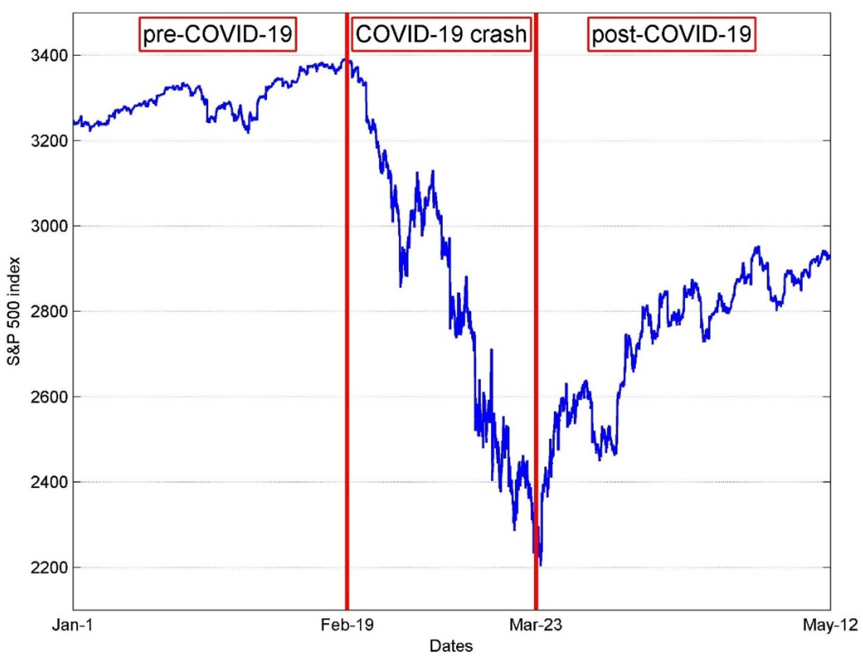
The data are at a five-minute frequency. Returns are calculated (rt = ln(Pt) − ln(Pt−1)) across each five-minute interval for seven asset classes (SPX, VIX, FX, OIL, GOLD, BTC, and TBILL) from 1 January 2020 to 12 May 2020, for a total of 7594 observations per asset class. The data are obtained from the Thomson Reuters Eikon terminal. We divided the data across three regime shifts during the 2020 market crash (Figure 1). The first period spans from 1 January–19 February, just before the 2020 market crash. We label this period the normal market regime. The second period spans from 20 February–23 March, representing the peak to trough of the 2020 market crash as measured by the SPX. We label this period as the market crash regime. The third period spans from 24 March–12 May, representing the recovery from the 2020 market crash trough. We label this period as the market recovery regime.
Table 1 presents the summary statistics for all seven asset classes. We note that in the pre-COVID-19 period, the average SPX returns were positive (negative for the VIX). At the same time, excess kurtosis was present in all of the time series. However, during the COVID-19 crash, the mean SPX returns became negative (positive for the VIX). In contrast, the standard deviation and kurtosis generally increased for all assets. The post-COVID-19 period was marked by lower volatility and risk (VIX), except for the crude oil returns, which showed excessive volatility and high excess (negative) skewness and kurtosis.
3. Methods
In time series analysis, the most commonly used test for gauging causality in bivariate systems was devised by Granger (1969). This test evaluates the forecasting performance of one time series in predicting another in regard to the first moment of a time series. By definition, the testing procedure is linked to a specific data frequency, while neglecting the fact that, in financial markets, data generating processes typically contain multiple layers of information, with each layer corresponding to a particular frequency. Hence, in this paper, we utilize the method by Breitung and Candelon (2006), which allows us to account for data dynamics across a range of frequencies.
Causality analysis can be effective in monitoring systemic risk and financial contagion in financial markets. Recent literature demonstrates its ability to capture risk propagation among investors that transact in different geographical locations (or invest in different asset classes). For example, Billio et al. (2012), McMillan (2020) and Duarte and Eisenbach (2021) have adopted causality analysis as a proxy for return-spillover effects among various market participants and asset classes. In the context of the current paper, price spillover effects represent causal interactions (or relationships) of market participants that are based on time series’ first moments. In essence, we study the dynamics of the price discovery process in terms of how information (and related trading activity) produced in one asset class transmits across other asset classes owing to the degree of market distress at various stages of the COVID-19 pandemic.
The test for causality in the frequency domain by Breitung and Candelon (2006) originates from Geweke (1982) and Hosoya (1991). Let zt = [xt, yt]′ be a two-dimensional time series vector with t = 1, ..., T. It is assumed that zt has a finite-order VAR representation:
where Θ(L) = I − Θ1L − … − ΘpLp is a 2 × 2 lag polynomial with Lk zt = zt−k. It is assumed that the vector εt is white noise with E(εt) = 0 and E(εtεt′) = ∑, where ∑ is a positive definite matrix. Next, let G be the lower triangular matrix of the Cholesky decomposition G′G = ∑−1, such that E(ηtηt′) = I and ηt− = Gεt. The system is assumed to be stationary, implying the following moving average representation:
where and . Using this representation, the spectral density of xt can be expressed as:
This measure is zero if in which case it is said that y does not cause x at frequency ω. The following null hypothesis is used to test the hypothesis that y does not cause x at frequency ω:
Breitung and Candelon (2006) show that the null hypothesis is equivalent to a linear restriction on the VAR coefficients from the following equation:
The hypothesis is equivalent to the linear restriction:
where β = [β1, …, βp]’ and:
The ordinary F statistic for (8) is approximately distributed as . To assess the statistical significance of the causal relationship between asset returns, the causality measure for is compared to the 5% critical value of a -distribution with 2 degrees of freedom (5.99).
4. Empirical Results and Discussion
4.1. Causality
We present the results of the causality tests in Table 2. According to a battery of information criteria, the following VAR specifications were selected for the bivariate systems between the S&P 500 index returns (ΔSPX) and the other time series: the CBOE VIX index returns (ΔVIX)-VAR(4), the EUR/USD exchange rate returns (ΔFX)-VAR(12), NYMEX WTI crude oil returns (ΔOIL)-VAR(27), COMEX gold spot returns (ΔGOLD)-VAR(15), Bitcoin/USD returns (ΔBTC)-VAR(5), and Treasury Bill returns (ΔTBILL)-VAR(10).
We begin by discussing the results at the aggregate level. Table 2 reveals that the SPX returns cause returns in four other financial markets at specific frequencies (i.e., VIX, GOLD, OIL, and TBILL) during normal market conditions. In contrast, bi-directional causal relationships emerge during the market crash (i.e., between the SPX and the VIX, OIL, GOLD, and BTC). All of the bi-directional causal relationships disappeared during the market recovery, aside from the SPX and GOLD. Interestingly, OIL, BTC, and TBILL are all shown to cause the SPX during the market recovery, while the SPX only causes the VIX (for ω < 1.3) and GOLD (2.2 < ω < 2.5). Overall, we observe the SPX driving unidirectional relationships with other financial markets during normal market conditions, the emergence of bi-directional causal relationships during the market crash, and several unidirectional connections whereby other financial markets cause the SPX during the market recovery.
Next, we highlight the individual causal relationships among the SPX and other financial markets. First, we note that the SPX and BTC do not exhibit any causality across any data frequency during normal market conditions. However, there is partial bi-directional causality between BTC and SPX during the market crash. Specifically, BTC causes SPX across all data frequencies. The SPX causes BTC across a narrow range of frequencies between 14 and 35 min (0.9 < ω < 2.2). During the market recovery, BTC continues to cause the SPX across all data frequencies. In contrast, the SPX no longer exhibits a causal relationship with BTC at any frequency.
Another intriguing finding emerges from the SPX and OIL, whereby the SPX causes OIL during the normal market regime at a wide range of higher and lower frequencies; however, this relationship shifts to OIL, causing the SPX at specific frequencies during the market crash (over a wide range of ω) and market recovery (over a narrow range of ω).
The SPX and GOLD also exhibit an interesting pattern of causal relationships across the three market conditions. The SPX has a causal relationship with GOLD across all three regimes. Specifically, the SPX causes GOLD at a narrow range of frequencies between 22 and 29 min during normal market conditions, across a wide range of frequencies during the market crash, and at a narrow range of frequencies between 12 and 14 min during the market recovery. Conversely, GOLD does not cause the SPX during normal market conditions. Still, it does exhibit a causal relationship during the market crash at frequencies greater than 12 min and at frequencies between 29 and 35 min during the market recovery.
The SPX is shown to have a causal relationship at specific frequencies with TBILL during normal market conditions and the market crash; however, the causal relationship’s direction switches to TBILL, causing the SPX during the market recovery.
The SPX and VIX causality tests yield results that are more intuitive and expected. Specifically, we find that the SPX exhibits a causal relationship with the VIX at specific frequencies across all three market conditions; however, the VIX only causes the SPX during the market crash at data frequencies less than 21 min. Therefore, a bi-directional causal relationship at specific frequencies is only exhibited between the SPX and VIX during the market crash. A unidirectional causal relationship whereby the SPX causes the VIX is exhibited during normal market conditions and the market recovery.
Lastly, we only note a causal relationship between the SPX and FX during the market crash, whereby the SPX causes the FX at frequencies greater than 11 min.
4.2. Determinants of Recovery
Considering that the market recovery period findings suggest that other asset returns mainly drove the S&P 500 index returns during this period, this subsection aims to identify the covariates of stock market returns at high-frequencies. For this purpose, we employ the LASSO framework at the five-minute time resolution. The advantage of the LASSO regression is that it will select only the most significant covariates of the six considered.1
LASSO is an estimator that reduces the number of potential coefficients in the model, which improves prediction accuracy and model interpretability. It is a variant of the least-squares approach, which constrains the sum of the coefficients’ absolute values. The LASSO estimator can be written as:
where yi is the ith observation of the dependent variable, β0 is an intercept, xij is the ith observation of the jth explanatory variable, and βj is its corresponding coefficient, while ≡ is the L1 norm and s is a tuning parameter. When s is relatively large enough, the constraint on β has no effect. The model becomes the standard least-squares regression. However, for smaller (but positive) values of s, the estimated parameters are shrunken versions of their least-squares counterparts, with some βj’s often equal to zero. A cross-validation (CV) method is typically used for estimating the optimal value for s (as well as for the parameter below), and we will also follow this approach.
Equivalently, the LASSO optimization problem can be written in a Lagrangian form as follows:
We estimate the LASSO regression using the coordinate descent algorithm that involves two stages (Friedman et al. 2007). In the first stage, we estimate λ with ten-fold CV on the third subsample of data (24 March 2020–12 May 2020; 2894 five-minute observations), which we refer to as the market recovery period. In the second stage, from the estimate of λ, we estimate the vector of regression coefficients. We set equal observation weights of 1, while the number of values for selecting λ is 100. All time series are standardized to zero mean and unit variance, and, thus, no intercept is used.
Table 3 displays the LASSO estimates of the predictors ranked based on the absolute value of the coefficients. The left panel of Table 3 shows the coefficients from the standard LASSO model. In contrast, the coefficients in the right panel are based on the adaptive LASSO model that adds weights to the LASSO optimization problem to counteract the potential issue of LASSO estimates being biased (Zou 2006). Both LASSO approaches produce similar results, with the largest coefficients on the VIX returns (negative) and the EUR/USD exchange rate returns (positive). The positive coefficient on GOLD returns follows them. Finally, we observe a positive coefficient on the U.S. Treasury Bill returns. The coefficients on Bitcoin and oil returns are both equal to zero.
Figure 2 plots the LASSO results for each coefficient. The coefficient’s magnitude is measured on the vertical axis and the L1 norm is measured on the horizontal axis. One can track the significance of a coefficient as it changes horizontally in the positive direction (i.e., from left to right). Clearly, the first predictor that diverges from 0 is the VIX, followed by the exchange rate and GOLD returns. Essentially, Figure 2 and Table 3 suggest similar results.
In all, we reveal that the VIX returns had the largest (negative) effect on the stock market during the market recovery. In other words, a reduction in the global perception of risk played the most prominent role in the post-COVID-19 recovery, and it increased SPX returns. The inverse relationship is intuitive, as the VIX is sometimes referred to as the “fear index.”2 Based on the magnitude of LASSO coefficients, the recovery process was (positively) affected by the spillovers from the FX and GOLD markets. Firstly, it appears that international portfolio investments could, to a certain extent, explain the stock market recovery via the FX market’s order flows. The seemingly counterintuitive positive relationship between GOLD and SPX returns suggests that the market recovery was liquidity-driven. This was also the case during the aftermath of the 2008 financial crisis. The only other significant effect was observed from the U.S. Treasury Bill returns, and it was positive. Such a relationship was also documented in the post-2008 credit crisis period, and it was contributed to a series of quantitative easings by the Federal Reserve that caused both the stock and bond markets to rally. Surprisingly, we do not find any evidence of the spillover effects originating in the Bitcoin market. Such findings are consistent with James (2021), who reported that cryptocurrencies and equities displayed a lower degree of correlation in the post-COVID-19 period than the peak-COVID-19 period.
5. Conclusions, Limitations and Future Research
This paper presents new insights into intermarket links and the resulting market microstructure across financial markets measured by price spillovers around the COVID-19 market meltdown. Overall, the results reveal that information is shown to mostly flow from the SPX to other financial markets during normal market conditions, flow both ways during the market crash, and mostly flow from other financial markets to the SPX during the market recovery.
More specifically, based on the local minimum and maximum values of the S&P 500 index, we define three market regimes and study the causal interactions between the stock market and other asset classes. We find, during the pre-COVID-19 regime, stock market activity spillovers to oil, gold and t-bills markets. In addition, the movements in the S&P 500 index cause the VIX returns (for ω > 1.9, i.e., at high-frequencies). We do not document any price spillover effects with the FX and Bitcoin markets. The evidence that the stock market is a “leading indicator” and moves ahead of the real economy is not new.3 However, by documenting the same phenomenon for high-frequency data, we make an original contribution to the literature in this area.
Furthermore, we provide overwhelming evidence of distressed trading across asset classes with causalities running in multiple directions during the COVID-19 market crash. The most pronounced bi-directional market spillovers are found between the stock market, and the gold and Bitcoin markets. Clearly, investors were severely distressed during the market crash and moved their trades intermittently from stocks to gold and Bitcoin (and vice versa). Moreover, there exists a bi-directional causality relationship between the S&P Ye500 index and the VIX (i.e., from the SPX to the VIX for all ω ∈ (0, π); from the VIX to the SPX for ω < 1.5). As the VIX represents theoretical 30-day market expectations (or market sentiment) based on the S&P 500 index, its larger values indicate an increased risk that the market will make a large swing. The observed bi-directional causality could be interpreted as the impact of trading activity on market sentiment that is in the state of panic and distress, while such a market sentiment at the same time drives trading decisions and leads to more distress.
Finally, we uncover the microstructure mechanisms that were catalysts for the post-COVID-19 market recovery. The evidence shows that the null hypotheses that the OIL, GOLD, BTC and T-BILL returns do not cause the SPX returns at frequency ω are all rejected for various frequencies (ω) during the recovery period. Such spillover effects can be attributed to the regained confidence of investors as they shifted from other asset classes back to the stock market. Further, the LASSO model estimates indicate that the investor sentiment reflected in the aggregate perception of market risk (VIX) was crucial for the gains in the S&P index returns after 23 March 2020. Also, the FX and GOLD market returns were among the top three determinants of SPX returns during this period.
This study is not without limitations. First, based on this study, future researchers could develop a more theoretical model that explores the price spillovers among the different asset classes explored within this study. That is, theoretical linkages could be explored to develop a set of hypotheses to explore asset price spillovers around the COVID-19 market meltdown. Secondly, our study relies upon high-frequency data at the five-minute interval over a relatively short period of time (i.e., 1 January 2020 to 12 May 2020). Future researchers may explore asset price spillovers across a longer period of time, especially for the COVID-19 market recovery period, in order to conduct out-of-sample robustness tests for the generalizability of the results. Lastly, our study relies upon seven different asset classes. Future researchers may consider additional asset classes, such as longer-term bond or international equity markets.
As a result, additional research in this setting is meritorious due to the unprecedented nature of the COVID-19 pandemic and the resulting impacts on financial markets across the globe. To better understand the market sentiment around the COVID-19 market meltdown, future research could also explore the option contracts written on the SPX and BTC and a panel of technical indicators.
Author Contributions
Conceptualization, C.L. and N.G.; methodology, N.G.; software, N.G.; validation, N.G.; formal analysis, N.G.; investigation, C.L. and N.G.; resources, C.L. and N.G.; data curation, N.G.; writing—original draft preparation, C.L. and N.G.; writing—review and editing, C.L. and N.G.; visualization, C.L. and N.G.; supervision, C.L. and N.G.; project administration, C.L. and N.G. Both authors have read and agreed to the published version of the manuscript.
Funding
This research received no external funding.
Data Availability Statement
Not applicable.
Conflicts of Interest
The authors declare no conflict of interest.
| 1. | |
| 2. | For example, in an option pricing setting, Shafi et al. (2019) conclude that the S&P 500 index movements are negatively correlated with those of the VIX index. |
| 3. | For instance, a comprehensive discussion can be found in Næs et al. (2011). In short, investors trade stocks based upon their expectations of the future. Therefore, stock market activity may antcipate a market movement before the actual economy reacts. |
References
- Al-Awadhi, Abdullah M., Khaled Alsaifi, Ahmad Al-Awadhi, and Salah Alhammadi. 2020. Death and contagious infectious diseases: Impact of the COVID-19 virus on stock market returns. Journal of Behavioral and Experimental Finance 27: 1–5. [Google Scholar] [CrossRef]
- Baig, Ahmed, Hassan Anjum Butt, Omair Haroon, and Syed Aun R. Rizvi. 2020. Deaths, panic, lockdowns and US equity markets: The case of COVID-19 pandemic. Finance Research Letters 38: 101701. [Google Scholar] [CrossRef]
- Billio, Monica, Mila Getmansky, Andrew W. Lo, and Loriana Pelizzon. 2012. Econometric measures of connectedness and systemic risk in the finance and insurance sectors. Journal of Financial Economics 104: 535–59. [Google Scholar] [CrossRef]
- Bing, Tao, and Hongkun Ma. 2021. COVID-19 pandemic effect on trading and returns: Evidence from the Chinese stock market. Economic Analysis and Policy 71: 384–96. [Google Scholar] [CrossRef]
- Breitung, Jorg, and Bertrand Candelon. 2006. Testing for short- and long-run causality: A frequency-domain approach. Journal of Econometrics 132: 363–78. [Google Scholar] [CrossRef]
- Corbet, Shaen, Yang Hou, Yang Hu, Brian Lucey, and Les Oxley. 2020. Aye corona! the contagion effects of being named corona during the covid-19 pandemic. Finance Research Letters 38: 101591. [Google Scholar] [CrossRef]
- Corbet, Shaen, Yang Hou, Yang Hu, Les Oxley, and Danyang Xu. 2021. Pandemic-related financial market volatility spillovers: Evidence from the Chinese covid-19 epicentre. International Review of Economics &. Finance 71: 55–81. [Google Scholar]
- Coronado, Semei, Rebeca Jiménez-Rodríguez, and Omar Rojas. 2017. An Empirical Analysis of the Relationships between Crude Oil, Gold and Stock Markets. The Energy Journal 39: 193–207. [Google Scholar] [CrossRef]
- Dai, Peng-Fei, Xiong Xiong, Zhifeng Liu, Toan Luu Duc Huynh, and Jianjun Sun. 2021. Preventing crash in stock market: The role of economic policy uncertainty during COVID-19. Financial Innovation 7: 1–15. [Google Scholar] [CrossRef]
- Demir, Ender, Mehmet Huseyin Bilgin, Gokhan Karabulut, and Asli Cansin Doker. 2020. The relationship between cryptocurrencies and COVID-19 pandemic. Eurasian Economic Review 10: 349–60. [Google Scholar] [CrossRef]
- Deng, Guichuan, Jing Shi, Yanli Li, and Yin Liao. 2021. The COVID-19 pandemic: Shocks to human capital and policy responses. Accounting and Finance. Available online: https://onlinelibrary.wiley.com/doi/10.1111/acfi.12770 (accessed on 28 April 2021).
- Duarte, Fernando, and Thomas Eisenbach. 2021. Fire-sale spillovers and systemic risk. Journal of Finance 76: 1251–94. [Google Scholar] [CrossRef]
- Friedman, Jerome, Trevor Hastie, Holger Hofling, and Robert Tibshirani. 2007. Pathwise coordinate optimization. The Annals of Applied Statistics 1: 302–32. [Google Scholar] [CrossRef] [Green Version]
- Geweke, John. 1982. Measurement of linear dependence and feedback between multiple time series. Journal of the American Statistical Association 77: 304–24. [Google Scholar] [CrossRef]
- Granger, Clive W. J. 1969. Investigating causal relations by econometric models and cross-spectral methods. Econometrica: Journal of the Econometric Society 37: 424–38. [Google Scholar] [CrossRef]
- Granger, Clive W.J, Bwo-Nung Huangb, and Chin-Wei Yang. 2000. A bivariate causality between stock prices and exchange rates: Evidence from recent Asian flu. The Quarterly Review of Economics and Finance 40: 337–54. [Google Scholar] [CrossRef]
- Gu, Xin, Shan Ying, Weiqiang Zhang, and Yewei Tao. 2020. How do firms respond to COVID-19? First evidence from Suzhou, China. Emerging Markets Finance and Trade 56: 2181–97. [Google Scholar] [CrossRef]
- Gungoraydinoglu, Ali, Ilke Öztekin, and Özde Öztekin. 2021. The Impact of COVID-19 and Its Policy Responses on Local Economy and Health Conditions. Journal of Risk and Financial Management 14: 233. [Google Scholar] [CrossRef]
- Guo, Jin, and Tetsuji Tanaka. 2020. Dynamic Transmissions and Volatility Spillovers between Global Price and U.S. Producer Price in Agricultural Markets. Journal of Risk Financial Management 13: 83. [Google Scholar] [CrossRef]
- Guo, Hongfeng, Xinyao Zhao, Hang Yu, and Xin Zhang. 2021. Analysis of global stock markets’ connections with emphasis on the impact of COVID-19. Physica A: Statistical Mechanics and Its Applications 569: 125774. [Google Scholar] [CrossRef]
- Hastie, Trevor, Robert Tibshirani, and Jerome Friedman. 2009. The Elements of Statistical Learning: Data Mining, Inference, and Prediction. Springer Series in Statistics. New York: Springer. [Google Scholar]
- Hastie, Trevor, Robert Tibshirani, and Martin Wainwright. 2015. Statistical Learning with Sparsity: The Lasso and Generalizations. Boca Raton: Chapman and Hall/CRC. [Google Scholar]
- Hoang, Thi Hong Van, and Qasim Raza Syed. 2021. Investor sentiment and volatility prediction of currencies and commodities during the COVID-19 pandemic. Asian Economics Letters, 1. [Google Scholar] [CrossRef]
- Hong, Yongmiao, Yanhui Liu, and Shouyang Wang. 2009. Granger causality in risk and detection of extreme risk spillover between financial markets. Journal of Econometrics 150: 271–87. [Google Scholar] [CrossRef] [Green Version]
- Hosoya, Yuzo. 1991. The decomposition and measurement of the interdependence between second-order stationary process. Probability Theory and Related Fields 88: 429–44. [Google Scholar] [CrossRef]
- James, Nick. 2021. Dynamics, behaviours, and anomaly persistence in cryptocurrencies and equities surrounding COVID-19. Physica A: Statistical Mechanics and Its Applications 570: 125831. [Google Scholar] [CrossRef]
- Jiang, Yonghong, Gengyu Tian, and Bin Mo. 2020. Spillover and quantile linkage between oil price shocks and stock returns: New evidence from G7 countries. Financial Innovation 6: 1–26. [Google Scholar] [CrossRef]
- Keown, Callum. 2020. Gold and Stocks Have Been Moving Together for Weeks. Here’s What It Means. Barron’s. May 11. Available online: https://www.barrons.com/articles/gold-and-stocks-have-been-moving-together-for-weeks-heres-what-it-means-51589203866 (accessed on 20 June 2020).
- Kilian, Lutz, and Cheolbeom Park. 2009. The impact of oil price shocks on the U.S. stock market. International Economic Review 50: 1267–87. [Google Scholar] [CrossRef]
- Liu, Taixing, Beixiao Pan, and Zhichao Yin. 2020. Pandemic, mobile payment, and household consumption: Micro-evidence from China. Emerging Markets Finance and Trade 56: 2378–89. [Google Scholar] [CrossRef]
- Liu, Zhifeng, Toan Luu Duc Huynh, and Peng-Fei Dai. 2021. The impact of COVID-19 on the stock market crash risk in China. Research in International Business and Finance 57: 101419. [Google Scholar] [CrossRef]
- Maghyereh, Aktham, and Hussein Abdoh. 2020. Tail dependence between Bitcoin and financial assets: Evidence from a quantile cross-spectral approach. International Review of Financial Analysis 71: 101545. [Google Scholar] [CrossRef]
- Makin, Anthony J., and Allan Layton. 2021. The global fiscal response to COVID-19: Risks and repercussions. Economic Analysis and Policy 69: 340–49. [Google Scholar] [CrossRef]
- Marquez, Jaime, and Silvia Merler. 2020. A Note on the Empirical Relation between Oil Prices and the Value of the Dollar. Journal of Risk and Financial Management 13: 164. [Google Scholar] [CrossRef]
- McMillan, David G. 2020. Interrelation and spillover effects between stocks and bonds: Cross-market and cross-asset evidence. Studies in Economics and Finance 37: 561–82. [Google Scholar] [CrossRef]
- Mensi, Walid, Ferihane Zaraa Boubaker, Khamis Hamed Al-Yahyaee, and Sang Hoon Kang. 2018. Dynamic volatility spillovers and connectedness between global, regional, and GIPSI stock markets. Finance Research Letters 25: 230–38. [Google Scholar] [CrossRef]
- Næs, Randi, Johannes A. Skjeltorp, and Bernt Arne Ødegaard. 2011. Stock market liquidity and the business cycle. The Journal of Finance 66: 139–76. [Google Scholar] [CrossRef]
- Ortmann, Regina, Matthias Pelster, and Sascha Tobias Wengerek. 2020. COVID-19 and investor behavior. Finance Research Letters 37: 101717. [Google Scholar] [CrossRef]
- Padhan, Rakesh, and K. P. Prabheesh. 2021. The economics of COVID-19 pandemic: A survey. Economic Analysis and Policy 70: 220–37. [Google Scholar] [CrossRef] [PubMed]
- Park, June, and Eunbin Chung. 2021. Learning from past pandemic governance: Early response and public–Private partnerships in testing of COVID-19 in South Korea. World Development, 10. [Google Scholar] [CrossRef]
- Qin, Xiuhong, Guoliang Huang, Huayu Shen, and Mengyao Fu. 2020. COVID-19 pandemic and firm-level cash holding—Moderating effect of goodwill and goodwill impairment. Emerging Markets Finance and Trade 56: 2243–58. [Google Scholar] [CrossRef]
- Shafi, Khuram, Natasha Latif, Shafqat Ali Shad, and Zahra Idrees. 2019. High-frequency trading: Inverse relationship of the financial markets. Physica A: Statistical Mechanics and Its Applications 527: 121067. [Google Scholar] [CrossRef]
- Tisdell, Clement A. 2020. Economic, social and political issues raised by the COVID-19 pandemic. Economic Analysis and Policy 68: 17–28. [Google Scholar] [CrossRef]
- Xiong, Hao, Zuofeng Wu, Fei Hou, and RJun Zhang. 2020. Which firm-specific characteristics affect the market reaction of chinese listed companies to the COVID-19 pandemic? Emerging Markets Finance and Trade 56: 2231–42. [Google Scholar] [CrossRef]
- Xu, Liao, Jilong Chen, Xuan Zhang, and Jing Zhao. 2020. COVID-19, public attention and the stock market. Accounting and Finance. Available online: https://onlinelibrary.wiley.com/doi/full/10.1111/acfi.12734 (accessed on 1 May 2021).
- Yagi, Michiyuki, and Shunsuke Managi. 2021. Global supply constraints from the 2008 and COVID-19 crises. Economic Analysis and Policy 69: 514–28. [Google Scholar] [CrossRef]
- Zaremba, Adam, Renata Kizys, David Y. Aharon, and Ender Demir. 2020. Infected markets: Novel coronavirus, government interventions, and stock return volatility around the globe. Finance Research Letters 35: 1–7. [Google Scholar] [CrossRef] [PubMed]
- Zou, Hui. 2006. The adaptive lasso and its oracle properties. Journal of the American Statistical Association 101: 1418–29. [Google Scholar] [CrossRef] [Green Version]
Figure 1.
S&P 500 index market regimes.

Figure 2.
LASSO coefficient paths.


Table 1.
Summary Statistics.
| ΔSPX | ΔVIX | ΔFX | ΔOIL | ΔGOLD | ΔBTC | ΔTBILL | |
|---|---|---|---|---|---|---|---|
| Normal Market Regime | |||||||
| Mean (×10−6) | 9.210 | −97.90 | −2.470 | −29.50 | 7.800 | 71.00 | 0.168 |
| Standard deviation (×10−4) | 5.176 | 64.877 | 1.887 | 15.224 | 5.043 | 18.224 | 0.480 |
| Median (×10−6) | 27.00 | 0.000 | 0.000 | 0.000 | 11.50 | 51.70 | 0.000 |
| Skewness | −0.266 | 0.320 | 0.305 | 0.067 | −0.588 | −0.269 | 0.010 |
| Kurtosis | 5.100 | 7.627 | 8.556 | 7.209 | 16.530 | 13.905 | 2.864 |
| Market Crash Regime | |||||||
| Mean (×10−6) | −3.840 | 267.70 | −3.440 | −162.10 | −30.50 | −14.10 | 0.623 |
| Standard deviation (×10−4) | 39.286 | 163.123 | 6.526 | 60.548 | 16.832 | 51.075 | 0.622 |
| Median (×10−6) | −183.70 | 583.00 | 0.000 | −198.90 | −1.610 | 29.40 | 0.000 |
| Skewness | 0.525 | −0.668 | −0.157 | −0.174 | −0.140 | 0.389 | −0.598 |
| Kurtosis | 6.569 | 13.178 | 8.974 | 26.917 | 7.249 | 20.609 | 11.879 |
| Market Recovery Regime | |||||||
| Mean (×10−6) | 51.50 | −155.80 | 11.90 | 88.60 | 21.90 | 79.10 | −0.612 |
| Standard deviation (×10−4) | 19.155 | 63.263 | 4.465 | 1187.191 | 11.236 | 28.053 | 0.544 |
| Median (×10−6) | 85.50 | −307.30 | 0.000 | 0.000 | 51.20 | 82.70 | 0.000 |
| Skewness | 0.280 | 0.330 | 0.746 | −23.636 | −0.352 | 0.420 | −0.131 |
| Kurtosis | 10.041 | 4.843 | 9.422 | 1125.328 | 6.592 | 43.722 | 3.163 |
Notes: The Normal Market Regime subsample is from 2 January 2020 to 19 February 2020, the Market Crash Regime subsample is from 19 February 2020 to 23 March 2020, and the Market Recovery Regime subsample is from 24 March 2020 to 12 May 2020. The following time series at the 5-min sampling frequency are considered: S&P 500 index returns (ΔSPX), the CBOE VIX index returns (ΔVIX), the EUR/USD exchange rate returns (ΔFX), NYMEX WTI crude oil returns (ΔOIL), COMEX gold spot returns (ΔGOLD), Bitcoin/USD returns (ΔBTC) and Treasury Bill returns (ΔTBILL).
Table 2.
Causality tests.
| Normal Market Regime (1 January–19 February 2020) | Market Crash Regime (20 February–23 March 2020) | Market Recovery Regime (24 March–12 May 2020) | ||||
|---|---|---|---|---|---|---|
| Null Hypothesis | χ2 Statistic | Prob > χ2 | χ2 Statistic | Prob > χ2 | χ2 Statistic | Prob > χ2 |
| ΔSPX does not cause ΔVIX at frequency ω | For ω > 1.9 | Reject | For all ω ∈ (0, π) | Reject | For ω < 1.3 | Reject |
| ΔVIX does not cause ΔSPX at frequency ω | For all ω ∈ (0, π) | Do not reject | For ω < 1.5 | Reject | For all ω ∈ (0, π) | Do not reject |
| ΔSPX does not cause ΔFX at frequency ω | For all ω ∈ (0, π) | Do not reject | For ω > 2.8 | Reject | For all ω ∈ (0, π) | Do not reject |
| ΔFX does not cause ΔSPX at frequency ω | For all ω ∈ (0, π) | Do not reject | For all ω ∈ (0, π) | Do not reject | For all ω ∈ (0, π) | Do not reject |
| ΔSPX does not cause ΔOIL at frequency ω | For ω < 0.3, 1.7 < ω < 2.0, 2.2 < ω < 2.3 | Reject | For all ω ∈ (0, π) | Do not reject | For all ω ∈ (0, π) | Do not reject |
| ΔOIL does not cause ΔSPX at frequency ω | For all ω ∈ (0, π) | Do not reject | For ω < 0.1, 0.5 < ω < 0.6, 1.8 < ω < 1.9, 2.3 < ω < 2.5, 2.9 < ω < 3.0 | Reject | For 1.4 < ω < 1.5 | Reject |
| ΔSPX does not cause ΔGOLD at frequency ω | For 1.1 < ω < 1.4 | Reject | For ω < 0.3, 0.6 < ω < 0.9, 2.3 < ω < 2.4, ω > 2.9 | Reject | For 2.2 < ω < 2.5 | Reject |
| ΔGOLD does not cause ΔSPX at frequency ω | For all ω ∈ (0, π) | Do not reject | For ω > 2.6 | Reject | For 0.9 < ω < 1.1 | Reject |
| ΔSPX does not cause ΔBTC at frequency ω | For all ω ∈ (0, π) | Do not reject | For 0.9 < ω < 2.2 | Reject | For all ω ∈ (0, π) | Do not reject |
| ΔBTC does not cause ΔSPX at frequency ω | For all ω ∈ (0, π) | Do not reject | For all ω ∈ (0, π) | Reject | For all ω ∈ (0, π) | Reject |
| ΔSPX does not cause ΔTBILL at frequency ω | For 2.4 < ω < 2.5, ω > 3.0 | Reject | For 1.2 < ω < 1.5, ω > 2.7 | Reject | For all ω ∈ (0, π) | Do not reject |
| ΔTBILL does not cause ΔSPX at frequency ω | For all ω ∈ (0, π) | Do not reject | For all ω ∈ (0, π) | Do not reject | For ω < 0.9, 1.5 < ω < 1.7 | Reject |
Notes: The null hypothesis is that y does not cause x at frequency ω. The following means that there is no causality at any data frequencies: “For all ω ∈ (0, π): Do not reject”. The following means that there is always causality at all data frequencies: “For all ω ∈ (0, π): Reject”. To find the actual data frequency at which the null hypothesis is rejected/not rejected, find (2π/ω), where the basic frequency is 5-min. For instance, if ω > 1.9, this represents data frequencies that are (2π/ω) = 3.3 × 5 min = 16.5 min; then the ω > 1.9 range corresponds to frequencies with a wavelength that is shorter than 16.5 min.
Table 3.
Estimated coefficients of the LASSO model.
| LASSO | Adaptive LASSO | |||
|---|---|---|---|---|
| Rank | Variable | Coefficient | Variable | Coefficient |
| 1 | ΔVIX | −0.9169 | ΔVIX | −0.9289 |
| 2 | ΔFX | 0.0584 | ΔFX | 0.0655 |
| 3 | ΔGOLD | 0.0557 | ΔGOLD | 0.0628 |
| 4 | ΔTBILL | 0.0178 | ΔTBILL | 0.0234 |
| 5 | ΔBTC | 0.0000 | ΔBTC | 0.0000 |
| 6 | ΔOIL | 0.0000 | ΔOIL | 0.0000 |
| R2 | 0.6273 | 0.6272 | ||
Publisher’s Note: MDPI stays neutral with regard to jurisdictional claims in published maps and institutional affiliations. |
© 2021 by the authors. Licensee MDPI, Basel, Switzerland. This article is an open access article distributed under the terms and conditions of the Creative Commons Attribution (CC BY) license (https://creativecommons.org/licenses/by/4.0/).
Share and Cite
MDPI and ACS Style
Lento, C.; Gradojevic, N. S&P 500 Index Price Spillovers around the COVID-19 Market Meltdown. J. Risk Financial Manag. 2021, 14, 330. https://doi.org/10.3390/jrfm14070330
AMA Style
Lento C, Gradojevic N. S&P 500 Index Price Spillovers around the COVID-19 Market Meltdown. Journal of Risk and Financial Management. 2021; 14(7):330. https://doi.org/10.3390/jrfm14070330
Chicago/Turabian StyleLento, Camillo, and Nikola Gradojevic. 2021. "S&P 500 Index Price Spillovers around the COVID-19 Market Meltdown" Journal of Risk and Financial Management 14, no. 7: 330. https://doi.org/10.3390/jrfm14070330