
Two Applications of the Analytic Conformal Bootstrap: A Quick Tour Guide


Department of Physics and Astronomy, Uppsala University, P.O. Box 516, SE-751 20 Uppsala, Sweden
*
Author to whom correspondence should be addressed.
Universe 2021, 7(7), 247; https://doi.org/10.3390/universe7070247
Submission received: 28 June 2021
/
Revised: 12 July 2021
/
Accepted: 13 July 2021
/
Published: 15 July 2021
(This article belongs to the Collection Women Physicists in Astrophysics, Cosmology and Particle Physics)
Abstract
:We reviewed the recent developments in the study of conformal field theories in generic space time dimensions using the methods of the conformal bootstrap, in its analytic aspect. These techniques are solely based on symmetries, particularly on the analytic structure and in the associativity of the operator product expansion. We focused on two applications of the analytic conformal bootstrap: the study of the expansion of the Wilson–Fisher model via the introduction of a dispersion relation and the large N expansion of the maximally supersymmetric Super Yang–Mills theory in four dimensions.
1. Introduction
Conformal field theories (CFTs) are ubiquitous in theoretical physics, as they play a crucial role in several setups spanning from statistical models and condensed matter physics to holographic theories. The symmetry group associated to conformal transformations in d space–time dimensions1 highly constrains the structure of the observables in these theories, completely fixing the space–time structure of two- and three-point correlators up to a set of coefficients (the conformal dimensions and the so-called three-point function coefficients). In contrast to ordinary quantum field theories, conformal field theories are equipped with a convergent operator product expansion (OPE) whose radius of convergence is finite. This structure allows us to write the product of two fields sitting in positions close to each other, as a linear combination of fields at a middle point. In particular, when inserted inside correlation functions, the OPE is particularly useful because it makes it possible to express n point functions as a sum over point functions. By repetitively using the OPE, it is then possible to reduce any n point function to a sum of two- and three-point functions. In addition, the OPE is associative and this property is crucial to obtain consistency conditions that constrain the two- and three-point coefficients, which is the set of quantities determining the dynamics of a CFT.
This approach goes under the name of the conformal bootstrap. Despite the fact that its original formulation goes back to the 1970s [1,2], a more recent numerical approach revived the interest in it [3]. The main idea is to use the associativity of the OPE inside four-point functions to be able to put numerical bounds on the conformal dimension and the three-point function coefficient (OPE data) of the lightest operator present in the OPE of the two operators appearing in the four-point function we started with. Over the years, these techniques proved to be extremely efficient and achieved impressive results, as can be seen in [4] for a recent review. This progress motivates a complementary analytic study of the consistency conditions, which exploits the analytic structure of the equations together with information on the OPE structure and additional symmetries, when present. This approach gave a plethora of results, for instance in the large spin sector [5,6] and in large N theories [7,8].
In this note, we review mostly the latter, the analytic approach. Despite their emergent simplicity, the crossing relations are very intricate equations, and in generic space–time dimensions, it is extremely complicated to systematically find solutions. Recently, this has been the focus of some investigations and it has become clear that an analytic approach can be developed to give powerful results. In this approach, it is possible to implement constraints that are more readily visible in Lorentzian rather than Euclidean signature. Namely, by focusing on a Lorentzian limit which selects the contribution from operators with large spin, crossing symmetry predicts their dimensions and three-point function coefficients. More precisely, in Lorentzian signature, one can take a limit in which the external operators are null separated. In this limit, the correlator develops singularities which, by crossing symmetry, are mapped to the OPE data of large spin operators [5,6,9]. The knowledge of the singularities allows us to compute the OPE data as an expansion in inverse powers of the spin. Crucially, this works on all orders, in practise allowing the full OPE data to be reconstructed just from singular terms. This approach turns out to be very efficient, particularly in large N theories where the corresponding singularities can be systematically computed. In particular, we discuss two applications of the analytic method: one based on the usage of a dispersion relation and the second one mainly targeted towards the study of four-dimensional superconformal theories.
The structure of the paper is as follows. In Section 2, the basics of conformal field theories are introduced, with a focus mostly on conformal bootstrap techniques and their implications. In Section 3, a dispersion relation for conformal field theory is introduced and the example of the correlators in the Wilson–Fisher models in dimensions is discussed. In Section 4, we introduced the basics of superconformal field theories, mostly focusing on four-dimensional theories and on the classification of the operators. In Section 5, we report the case of the four-dimensional = 4 super Yang–Mills theory and in particular, we present the methodology and the results to obtain the most transcendental piece of the graviton amplitudes in .
2. Basics of Conformal Field Theory
Conformal transformations are those transformations that locally preserve the angles between the curves. Under a conformal transformation in a d-dimensional space (), the metric tensor transforms as
where the function is known as the scale factor. Conformal transformations consist of the following infinitesimal transformations:
- Translation:
- Rotation:
- Dilatation:
- Special conformal transformation (SCT):
where is an antisymmetric tensor and are arbitrary vectors.
The finite conformal transformations corresponding to those infinitesimal ones along with the generators are given by
| Transformation | Generator |
| Translation: | |
| Rotation: | |
| Dilatation: | |
| SCT: | . |
The generators form the conformal algebra, whose commutation relations in flat spacetime are:
All the commutators that are not written above vanish. The conformal group is or in Euclidean or Lorentzian signature, respectively.
Conformal field theory (CFT) is described by an infinite set of local operators specified by their scaling dimension and spin ℓ in the symmetric traceless representation ( for the OPE of two scalar operators. It is customary to work with states that are eigenstates of the dilatation operator:
Here, is a state that is created by the action of a local operator of scaling dimension at the origin on the vacuum:
The states are in one-to-one correspondence with local operators in a CFT. Inserting a primary operator at the origin generates a state with scaling dimension and this is the so-called state-operator correspondence. In this article, we discuss unitary conformal field theories, which have bounds for the operator scaling dimension:
In addition, the action of and on the eigenstates of the dilatation generator increases and decreases the eigenvalue by unity, due to their mass dimensionality. If we keep acting with on these states, we will eventually reach a state with negative scaling dimension. For a unitary CFT, states with negative dimension are not allowed and we must have , after acting with a finite number of times. The operator that creates this state is called a primary operator of dimension . When acting n-times with on primary operators, it is possible to generate a tower of operators with dimension . These operators are called descendant operators.
In a CFT, the observables are the correlation functions of local operators. We can write the product of two local operators and of scaling dimensions and , respectively, as a sum over an infinite number of primary operators of scaling dimension . This is known as the operator product expansion (OPE):
where the coefficients depend on the positions of the operators as well as on their scaling dimensions and spins. This is a convergent expansion that is valid for the finite separation of the operators . Conformal symmetry determines the coefficients up to a numerical factor :
where are numbers completely fixed by conformal symmetry. We quote here these numbers for the special case and and d space–time dimension:
The coefficient is known as the OPE coefficient.
The power of CFT lies in the fact that it fixes the one-, two- and three-point functions, up to a set of coefficients and , with a fixed space–time dependence:
where is the scaling dimension of and . Note that the coefficients of the two-point function can be re-absorbed by redefining the fields and then the coefficients of the three-point functions cannot be further re-absorbed. The three-point function is fixed up to a constant . To see that this is the same number that appears in Equation (7), we apply the OPE Equation (6) to a three-point function and use the fact that the two-point function is non vanishing only when both operators are the same Equation (10). This kills the sum in Equation (6) to one operator and we are left with the form Equation (11).
The numbers that specify a CFT, namely the spectrum or scaling dimensions and the OPE coefficient of the operators, are known as the CFT data. If we know all of these CFT data, then we can completely fix the theory. The higher point correlation functions can be recursively computed reducing it to a lower point correlation function by using the OPE. In Equations (9)–(11), the operators are scalars (), but conformal symmetry fixes the correlators of spinning operators in a similar way.
Now let us consider the four-point function which is not fully fixed by conformal invariance and therefore encodes the dynamical information of the CFT. If we consider four identical scalars of scaling dimension , inserted at four different points, it is possible, using conformal symmetry, to write the four-point function in terms of conformally invariant cross-ratios defined as
The four-point function takes the following form:
where and ℓ denote the scaling dimension and spin of the operators O being exchanged. The coefficients are the square of the OPE coefficients . We will use the term OPE coefficient for in what follows. The function contains the contribution of a primary operator of dimension and all of its descendants. These are the conformal blocks whose form is completely fixed by conformal symmetry. They satisfy a differential equation derived from the conformal Casimir [10,11]. The conformal blocks are generally complicated functions of cross-ratios and the explicit representation is known as an integral representation. In even space-time dimension, some closed form expressions are known. We quote the form of the conformal blocks in four dimensions below:
where:
Here, is a Gauss hypergeometric function. Inside the four-point function Equation (13), we can fuse together operators (12) and (34). This is the s-channel expansion of the correlator. We could have also expanded into the t-channel where we fuse (14) and (23), or in the u-channel where we fuse (13) and (24). Since the OPE is associative, these three expansions must be the same. This is the statement of crossing symmetry which is fully equivalent to the associativity of the OPE, and results in the following equation:
This is the conformal bootstrap equation. The crossing symmetry is depicted in Figure 1. The conformal bootstrap is a self-sustaining process that is supposed to continue without any external input and entirely relies upon the symmetry of the CFT. We focus on the CFT itself without worrying about a specific microscopic realisation and this is a Lagrangian free approach. Equation (16) is a functional constraint on the CFT data and must be satisfied for all values of the cross-ratios . However, this is a complicated constraint as it involves a double infinite sums over the operator spectrum and spin. It is not possible to generically solve this equation analytically and extract the CFT data. There are several approaches to extract the CFT data by solving Equation (16), both analytical and numerical. One efficient method is the numerical one, which is a numerical procedure that allows finding bounds on the CFT data for the operators appearing in the OPE decomposition, by using the relation Equation (16) and other symmetries that the theory may possess, as can be seen for instance in a recent review [4]. In the next sections, we discuss some of the analytic methods to study the same relations [12].
3. Dispersion Relation in CFT
In this section, we present a dispersion relation for the CFT four-point correlation function following [12]. The dispersion relation makes it possible to construct a function from the knowledge of its discontinuity. We will exploit the analytic properties together with the crossing symmetry of the correlator Equation (16) and show that in perturbative CFT, where we have an expansion of the CFT data in a perturbative parameter, the four-point function only depends on the spectrum of the theory and the OPE coefficients of certain low lying operators2.
3.1. Analytic Structure of Conformal Blocks
Let us begin by analysing the analytic structure of the conformal blocks in d dimensions [13]:
where:
is the conformal block for the scalar exchange operators. The conformal blocks for the exchange of spinning operators can be obtained from the scalar blocks by a recursion relation [13]. The sum over n in Equation (18) results in a hypergeometric function. One can further use the Euler integral representation for the hypergeometric function and rewrite Equation (18) in the following form
In what follows, we will study the analyticity in the variable z and keep fixed to some value between 0 and 1. Note that lies on the u-channel branch cut which is on the boundary of the convergence region of the u-channel. It was shown in [15] that the OPE converges in this regime in a distributional sense. Hence, the domain of analyticity in z becomes:
The conformal blocks for the exchange of spinning operators inherit the same analytic properties as they are given in terms of Equation (18) by a recursion relation in ℓ. The conformal blocks have this specific structure in any space–time dimension.
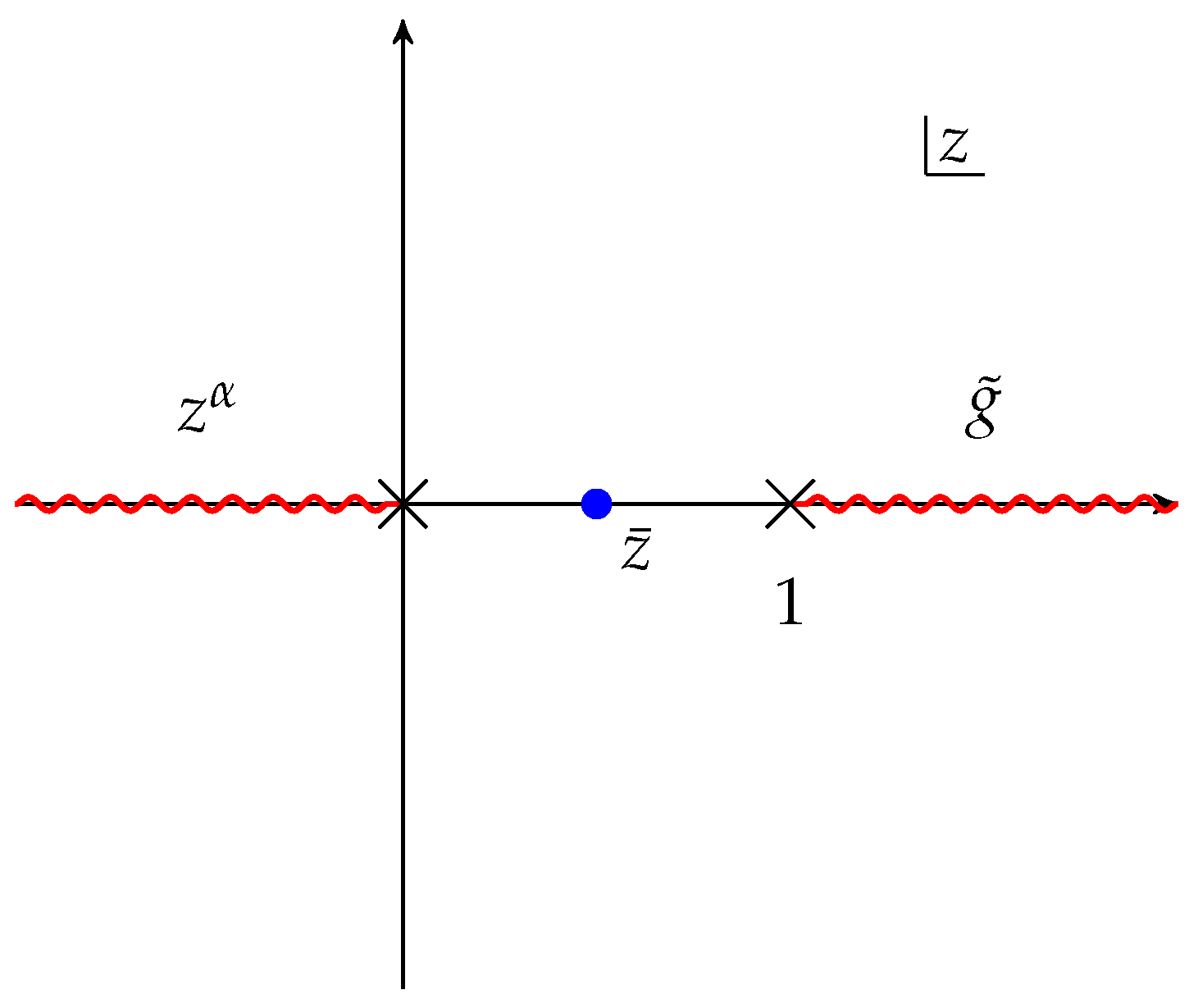
The conformal blocks Equation (17) have a branch cut for that originates from the non-integer powers of z. The blocks have another branch cut for originating from . The analytic structure of the conformal block is depicted in Figure 2. Note that the discontinuity of the branch cut due to the overall power in the second line of Equation (13) is much simpler, which results in:
where we define the discontinuity of a function as
We will see how Equation (22) plays a key role in the CFT dispersion relation in the next sections.
3.2. Crossing Symmetry and Dispersion Relation
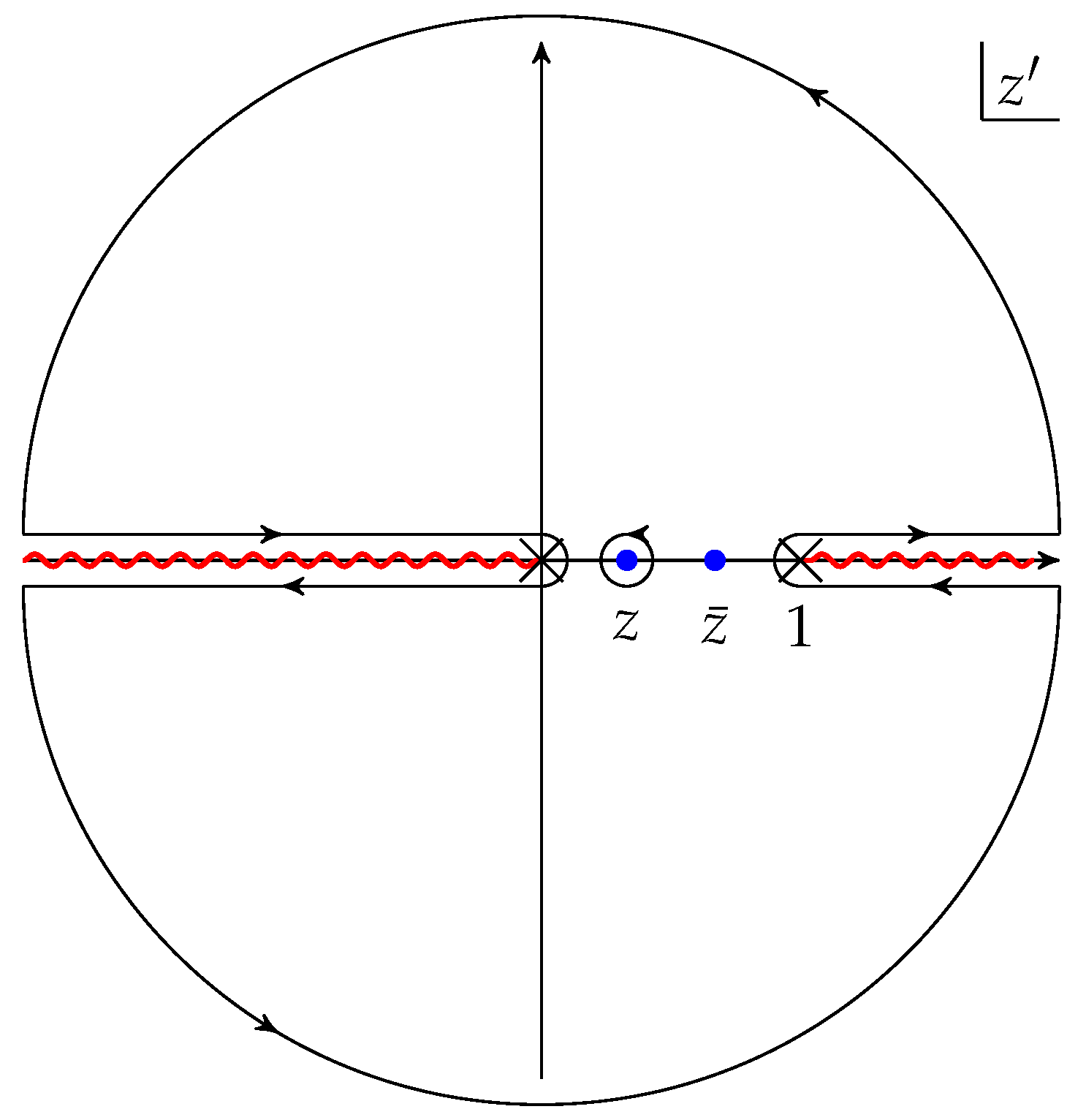
In this section, we exploit the analytic properties and crossing symmetry of the conformal correlator to present a dispersion relation. As a first step, we introduce a pole at a generic point and write the correlator Equation (13) as the residue of this pole using Cauchy’s residue theorem:
The analytic structure of this correlator follows from the analytic structure of the conformal blocks as discussed in the previous section. Now, we deform the contour to wrap around the branch cuts on the real axis as shown in Figure 3. In order to determine the arc contribution at , we have to consider the Laurent series expansion of , which is given by the u-channel OPE:
Note that due to the overall prefactor , only primary operators with contribute to the arc at infinity. However, for unitary CFTs in , the unitary bound Equation Equation (5) shows that identity () is the only such operator that contributes to the arc and its arc contribution is 13. This results in the following dispersion relation:
Now, we use the crossing symmetry Equation (16) to express the discontinuity at in terms of the simpler discontinuity at :
This can be used to rewrite the integral on the positive real axis in Equation (26) in terms of an integral on the negative real axis:
Putting these together, we obtain the following dispersion relation:
This shows that the correlator in a unitary CFT is determined by its discontinuity at together with crossing symmetry.
Let us see how the dispersion relation can be applied to compute correlators in a mean field theory in d dimensions. We assume that the identity operator is present in the OPE of the operators. Now, we show how the identity operator in the s channel reproduces the mean field theory correlator. The s channel identity is given by , whose discontinuity is:
Using Equation (29), we obtain the following mean field theory correlator:
Note that plugging Equation (30) into Equation (29) will yield a finite result for . For , the prefactor in Equation (30) vanishes. The discontinuity in that case, coming from a pole, is a delta function and can be thought of as a distribution around which finally yields the same result as in Equation (31). However, one needs to analytically continue in order to obtain Equation (31) for generic values of . This analytic continuation is justified in perturbation theory where we have analytic control. The way to obtain the analytic continuation in general is to consider a subtracted dispersion relation which is not what we did. In that sense, the use of this dispersion relation is limited.
Now, we can decompose Equation (31) into conformal blocks:
to reproduce the mean field theory OPE coefficients [16]:
Note that only even spin operators appear in the OPE when we study the correlator of four identical scalar operators.
We will now study perturbative CFT, where we have an expansion around the mean field theory in the perturbative parameter . The exchanged operators in the operator product expansion of contain double trace operators of the schematic form with bare dimension . We begin by expanding the CFT data as follows:
This results in the following expansion of the correlator:
The leading order correction to the correlator is given by
where is the derivative of with respect to . We compute the discontinuity of Equation (36) at using Equation (22):
Using Equation (29), we can compute the correlator . Since Equation (37) determines the correlator from the dispersion relation, it follows that the CFT correlator in perturbative settings is entirely determined by the spectrum at that order and the OPE coefficient at the previous order in the CFT. As a next step we can decompose the correlator into conformal blocks and extract the OPE coefficient . This process is summarised in Table 1.
3.3. Computing Wilson–Fisher Correlator Using Dispersion Relation
In this section, we discuss how the dispersion relation Equation (29) can be applied to compute the four-point correlation function in Wilson–Fisher theory in dimensions as a perturbative expansion in . The Wilson–Fisher theory is described by the Lagrangian:
where is the energy scale and we have a fixed point for the coupling . The correlator in the theory can be computed by perturbatively evaluating Feynman diagrams in the -expansion. Here, we will compute the correlator using Equation (29). The correlation function and the CFT data contain the same amount of information. However, it may not always be possible to resum the CFT data and obtain a closed form expression for the correlator. It is easier to extract the CFT data from the closed form expression of the correlator. We will see that the dispersion relation allows us to directly compute the correlator without resumming the CFT data. In perturbative CFT, this can be thought of as an alternative way of computing the correlator using the inputs (spectrum) from the Feynman diagrams. The inputs we need here can be obtained from the two-point function which is much simpler to compute than the four-point function.
We expand the CFT data in using the input from Wilson–Fisher theory:
From Equation (33), it is evident that only operators appear in the OPE up to :
Since the anomalous dimensions of operators start at , only the operator will contribute to the discontinuity of the correlator at . The associated discontinuity from is given by
Using Equation (29), we obtain:
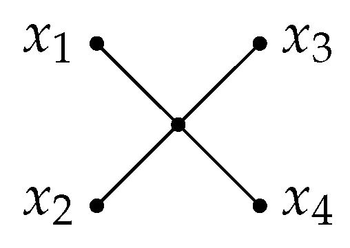
This corresponds to the contact diagram Figure 4. The correlator Equation (44) can be decomposed into conformal blocks to obtain the following OPE coefficient:
Now, we proceed to compute the correlator at the next order. Since we are only interested in the terms having discontinuity at we expand the correlator as follows:
The discontinuity of at reads:
We can evaluate the ℓ sum above using the explicit form for the conformal blocks in four dimensions:
where is defined in Equation (15). This results in:
Then, we evaluate the first order expansion of the conformal block using the expression for general dimension:
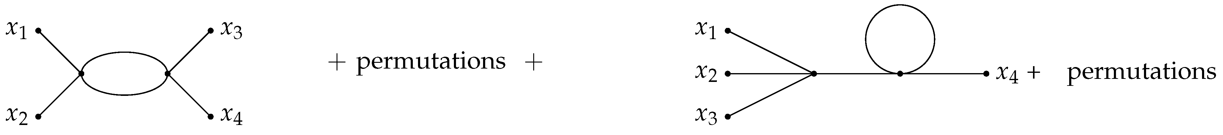
Putting all the terms together in Equation (48), we finally compute the correlator from Equation (29):
This correlator corresponds to the diagrams in Figure 5.
Now, we decompose the correlator into conformal blocks to evaluate the OPE coefficients which is in agreement with [17]:
and [18]:
Here, is the harmonic number of order ℓ.
To summarize, in this section, we show that it is possible to use a dispersion relation which, together with crossing symmetry, specifies the OPE coefficients as a function of the conformal dimension, in theories that admit a perturbative expansion.
4. Basics of Superconformal Field Theory
We will now see what changes in this description when a theory is not only conformal invariant but also supersymmetric and we enter the realm of superconformal field theories (SCFTs). The presence of additional symmetry will even further constrain the spectrum of these theories and it will further help the analysis of correlation functions, unveiling new and interesting properties. From this moment onwards, we will focus on space–time dimensions, which will be relevant for the following4.
When supersymmetry (SUSY) is in play, one needs to change and generalize the commutation relations in (2) to allow for the presence of supersymmetry generators, namely the supercharges and , with being the spinor indices. The index i takes values from 1 to , which corresponds to the amount of supersymmetry; in four space–time dimensions and restricting to theories whose particles have spin up to 1, ranges from 1 to 4, where the latter corresponds to maximal supersymmetry. By studying the interplay between these supercharges and the conformal generators, one realises that in order to have a closed algebra, it is necessary to add some other fermionic generators, the conformal supercharges and .
Supersymmetry usually comes together with an additional symmetry that allows to rotate between supercharges, which is known as R-symmetry. Its generators organise in a algebra for or a algebra for . A distinguishing characteristic of SCFTs is that in this case, the R-symmetry it is not an outer automorphism of the Poincaré SUSY algebra, as it happens in the non-conformal supersymmetric case, but it is really part of the algebra, as it commutes with the conformal subalgebra and acts non-trivially on the supercharges. All in all, the combination of conformal generators, Q’s, S’s and defines a simple Lie superalgebra: for and for . They contain, respectively, as bosonic subalgebras and , where in the first term of both expressions, we recognize the usual conformal algebra in four dimensions. We will label operators based on how they transform under this subset: we will specify their conformal dimension , Lorentz quantum numbers and R-symmetry charges, encoded in the Dynkin labels of and charge when present.
Operators can be further organised into superconformal primaries (or superprimaries) and superdescendants. An operator is a superprimary if:
Since schematically , a superprimary is in particular a conformal primary, but we notice that the converse is not true. This implies that in a given superconformal representation, we can potentially find many conformal primaries. Superdescendants are obtained from a superprimary by acting with the Q’s, also in this case, the usual notion of conformal descendant is recovered thanks to the relation . The combination of a superprimary and all its descendants forms a superconformal multiplet.
The last thing left to discuss is how the unitarity bounds in Equation (5) change in the presence of SUSY. It can be argued that the presence of additional symmetry should determine even stronger constraints.
Suppose that there exists an unitarity bound given by some function , where R stands for R-symmetry quantum numbers, then we can distinguish [20,21]:
- Superprimaries with which give rise to long multiplets. In general, a long multiplet contains states;
- Operators at the unitarity bound and operators with , but still allowed for specific spins and R-charges. These form short multiplets, so called because they obey some “shortening conditions” that are concretely realized in the fact that they are annihilated by a certain amount of Q’s and ’s, and hence, the multiplet can only contain a reduced number of states. These operators are often called BPS and their dimension, being determined by Lorentz and R-symmetry quantum numbers, is protected against quantum corrections5.
5. = 4 Super Yang–Mills
In this section, we will analyse how the bootstrap techniques have been employed to study and powerfully constrain the spectrum and correlators of super Yang–Mills (SYM) theory in four dimensions. One reason to study such theories is that, through the AdS/CFT correspondence [22,23,24,25], it is holographically related to Type IIB string theory on AdSS, where the CFT should be thought as living on the AdS boundary. The precise form of the duality reads
![Universe 07 00247 i001]()

One of the checks that have been made to justify and investigate the validity of this correspondence is verifying that the symmetries present on the two sides actually match. Furthermore, indeed, restricting to the bosonic part of the superconformal group, we find that the conformal symmetry is reproduced by the isometries of AdS, while the R-symmetry group is recovered as the isometries of the five-sphere.
The AdS/CFT correspondence is conjectured to hold for any value of the parameters characterising the two theories and listed beforehand. However, it is useful to study two particular limits [26], which are the ones most widely used; for this purpose, let us introduce the ’t Hooft coupling [27]. First of all, let us take N to infinity while keeping fixed; in this limit, usually called ’t Hooft limit, the large N limit of the SCFT is mapped to weak coupling string perturbation theory, where each correction in powers of should be interpreted as a specific genus in the corresponding expansion. Then, we can further take , but still less than N: in this second regime, the correspondence reduces to the one between strongly coupled SYM and Type IIB supergravity on weakly curved AdSS.
Now, that we introduced the general framework in which SYM can be inserted, let us delve further into the spectrum and properties of this theory.
5.1. Operators and Spectrum
SYM is believed to be, even if it is not yet proved, the unique theory with the maximal possible amount of supersymmetry6 in four dimensions. The massless elementary fields of the theory are a gauge vector , four Weyl fermions and six real scalars . They can all be rearranged to form a supermultiplet, the gauge multiplet, and as the name suggests, they transform into the adjoint of the gauge group. Under the R-symmetry group, is a singlet, transforms into the of and into the fundamental of or equivalently as a rank 2 antisymmetric tensor of .
Given the fundamental constituents of the theory, it is possible to write explicitly a Lagrangian [26,28] and verify that this is indeed a conformal invariant and supersymmetric, at least classically. Quite remarkably, SYM does not suffer from any perturbative UV divergences7 at the loop level, and as a consequence, there is no need to introduce any scale during the renormalisation procedure, and hence, the function vanishes identically in the full quantum theory. This tells us that SYM is exactly a superconformal field theory and is a full quantum symmetry.
To classify the spectrum of the theory, we should construct all possible local, gauge invariant operators made of the canonical fields introduced above. Among these are superprimary operators, as defined in Section 4, which can be constructed as the symmetric product of the elementary scalars . The simplest configuration leads to single trace operators of the form:
where we are taking the symmetrized trace (str) over , which makes the operator symmetric under the indices as well. In general, Equation (56) defines a reducible representation and one has to further distinguish between the trace and the traceless part of it. In the easiest example, by doing so, we can differentiate between the Konishi operator, , and , where singles out the traceless part. The products of these single trace operators constitute multi-trace operators.
As anticipated in Section 4, it is convenient to classify states/operators according to the unitary representations of the bosonic subalgebra:
In addition to these quantum numbers, we will specify whether they satisfy some shortening conditions. Interesting types of operators that will be relevant for what follows are:
- Identity operator, which is a singlet of R symmetry and it has ;
- -BPS operators, scalars annihilated by half of the supercharges. They can either be single trace operators:symmetric traceless tensors transforming in the or multi-trace operators:where stands for projection into the corresponding representation. Their dimension is protected from quantum corrections and supersymmetry completely fixes their three-point functions [26,29,30,31,32,33,34].
- -BPS operators , with Dynkin labels and protected dimension and -BPS operators, multi-trace operators in the having fixed dimension . Both these types are genuinely BPS only in the free theory and mix with descendants of non-BPS operators when interactions are turned on.
- Long operators can transform into a generic R-symmetry representation, as their dimension is not protected but nonetheless subject to the unitarity bound:
In light of the AdS/CFT correspondence, it is possible to establish a dictionary between these operators and fields in the dual AdS, after having compactified along S [22,35]. Single trace operators are mapped to single particle states, in particular , which is dual to the scalar of the graviton supergravity multiplet, while correspond to its Kaluza Klein modes. The masses of these supergravity scalars are completely fixed by the conformal dimension of their duals as . Multi-trace operators, on the other side, are mapped to threshold multiparticle bound states in AdS. Let us conclude by mentioning that it can be shown that some other non-BPS operators, such as the Konishi multiplet, scale as : these operators correspond to massive string modes that decouple in the supergravity regime , which is the one we are mainly interested in.
5.2. Stress Tensor Multiplet Correlators
As we were mentioning before, the two- and three-point functions of -BPS operators are completely fixed by superconfomal symmetry and do not receive quantum corrections thanks to some non renormalisability theorems [36,37,38,39,40,41]. The four-point function instead enjoys only partial renormalisability and therefore it does depend on the coupling constant but just through a trivial function [42,43,44,45,46]. Thanks to this property, the four-point function of any superdescendant is determined by the one of the corresponding superprimary. Therefore, it is enough to study the correlators of superprimaries, in general, easier since they involve scalars, to constrain correlators of superdescendants. This turns out to be incredibly useful if one wants to study supergravity. Studying graviton amplitude amounts to compute correlators of the stress tensor is generally difficult to do. However, the stress tensor belongs, together with R-symmetry and super currents, to a -BPS multiplet, whose superprimary is the single trace operator introduced before. Thus, we can focus on and that is why we will devote the rest of the section to its analysis. In particular, we will see how to “bootstrap” this correlator, meaning employing all the available symmetries to constrain its form and obtaining information about the spectrum of our theory [45,46,47,48,49].
is a scalar of protected dimension and it transforms into the representation of an R-symmetry group, thus as a symmetric traceless tensor. To ensure this one can introduce , null vectors , , and rewrite:
As already mentioned, it is the superconformal primary of the supermultiplet to which the stress energy tensor belongs.
Conformal symmetry on its own already partially fixes the form of its four-point function to be:
where u and v are the conformal cross ratios introduced in Equation (12). Then, we can enforce symmetry: this imposes constraints on the possible representations that can be exchanged in the OPE:
Such decomposition allows us to rewrite:
where label the six representations exchanged in Equation (61). The functions are harmonics, which can be written in terms of Legendre polynomials and depend on the polarization cross ratios [49]:
Notice that for the correlator of four, dimension two, operators is a polynomial of degree 2 in and .
Since we are considering the correlation function of identical operators, we need to impose invariance under permutations of all external operators. This translates into the following crossing equations for the function :
These requirements can be read as well as consistency conditions for the , which admits an expansion in the usual conformal blocks8:
where the 4D conformal blocks have been defined in Equations (14) and (17)9. Notice that the sum runs over the spin ℓ because in the OPE of two scalars, the exchanged operators can only be symmetric traceless Lorentz tensors, for which with ℓ even. As already discussed before expanding, conformal blocks allow us to packing together the contribution of each conformal primary and all its descendants. However, in the presence of supersymmetry10, we would like to expand the correlator in such a way that each supermultiplet contributes to the OPE as a whole; in other words, we would like to find some superconformal blocks condensating the contribution of each superprimary and all its descendants. This is in general very hard, however, it is possible in this case by fully exploiting the power of superconformal invariance and solving superconformal Ward identities. These identities can be phrased as [49]
with analogous requirements for . The function f encodes the contribution from the protected sector of the theory, namely from all the possible short and semi-short representations that can be exchanged in the OPE, and for this reason, can be completely determined by free field theory results. It has to satisfy the consistency condition , where k is a generic constant and in light of this, it can be rewritten as
In a complementary interpretation [46,50], arises from the appearance of an additional chiral structure, which is a general property of superconformal field theories but can be extended to as well. In this picture, can be understood as a correlator of a two-dimensional auxiliary chiral algebra.
A generic solution of the Ward identity in Equation (67) can be written as
contains the dynamical information of the theory and encodes the contribution from long supermultiplets. In the special case of external dimension , it does not depend on the cross ratios. Remarkably, it is possible for it to find a decomposition in superconformal blocks:
where it turns out that a superconformal block is just a usual block with a shift by 4 in the dimension. The exchanged operators are long supermultiplets whose lowest dimension operator is a singlet of . Furthermore, the function admits a similar expansion:
where the coefficients are known [49] and we introduced blocks . Here, only short representations, whose dimension can be fixed in terms of the spin, contribute. These decompositions in superconformal blocks make manifest the contributions of the various types of multiplets. However, there is still an intrinsic ambiguity due to the fact that at the unitarity threshold, long multiplets decompose into short and semi-short ones and in a non-interacting theory, there is no way to distinguish truly protected from unprotected contributions. It is indeed common to further distinguish:
where we stripped out the contributions coming from the protected sector in , which is explicitly known, as can be seen in [46]. can still be expanded as in Equation (70):
where now the sum is over unprotected long operators, singlet of R-symmetry, with and , as expected from unitarity.
The crossing conditions in Equation (65) becomes:
where is the central charge of the theory and is linear in .
To date, we have seen how symmetries give stringent constraints on the form of the four-point function and can already give information about the protected spectrum of the theory. However, there are still undetermined data hidden in and one would like to find a way to study the dimensions and the squared OPE coefficients appearing there. Various approaches have been pursued in the years, from numerical bootstrap techniques [45,46,51,52,53] to the more analytic ones [54,55,56,57,58,59,60,61,62,63,64,65,66], involving the use of modern tools such as the Lorentzian inversion formula [9,67,68], large spin perturbation theory [5] and unitarity methods [8,69]. These studies have shed some light on the spectrum of long operators in and they have provided non-trivial tests of the AdS/CFT correspondence, especially in the large N (or equivalently large ) limit and at infinite ’t Hooft coupling . In this limit, the interacting part of the correlator can be expanded as
where each term maps to a loop in the dual gravity amplitude11.
As discussed before, in this regime, corresponding to the supergravity approximation, all string modes become infinite massive and we are left with protected single trace operators and long multi-particle ones, which are dual to multi-trace operators in the dual picture. The latter receive corrections both to their dimensions and OPE coefficients at large N. Among them, the only ones with a non-zero anomalous dimension and three-point coefficient already at order are double trace operators12. They are constructed from the product of -BPS operators and they take the schematic form and at leading order, and they assume their classical dimension is . Their OPE data admit an expansion similar to Equation (75):
where we introduced the twist and we denoted with the anomalous dimension at order . Notice that for fixed n and ℓ there, can be more than one superconformal primary with the same twist and transforming in the same representation.
By plugging Equations (76) and (77) in the expression for in Equation (73), we can express the single in terms of anomalous dimensions and corrections to the OPE coefficients. The first few terms are given by
The quantity in the first line can be derived from disconnected diagrams in free field theory and allows to fix:
An explicit expression is also known at order in terms of so-called function [13,70]:
where both h and admit an expansion in power of u if we allow for negative powers in . By matching with the logarithmic part in Equation (79), one can extract the anomalous dimension of double trace operators at order :
and analogously, from , one can obtain:
Going to a higher order, we inevitably run into problems due to mixing among degenerate double trace operators, since all operators of the form will equally contribute to Equation (76). In light of this, the tree level information only fixes for us the averages, over all these degenerate states, of the various OPE data; however, at one loop (and higher), powers and products of these data appear, so that computing them requires unmixing the different contributions. Therefore, let us introduce an additional index I to account for the degeneracy and define new with to be eigenfunctions of the dilatation operator. Solving this mixing problem then requires computing and for each index I, order-by-order in the large c expansion. Remarkably, this has been done at order and partially at by studying mixed correlators in [54,55,56,59], providing as with explicit expressions for and .
A closer look to Equation (80) shows us that this knowledge is sufficient to completely reconstruct one piece of the correlator, namely the leading one:
where this expression can be explicitly resummed in terms of logarithms and polylogarithms times some rational functions [55]. However, the importance and relevance of this term is not limited to the possibility of computing it, which is still quite extraordinary; rather, it relies on the fact that this is enough to extract information on and eventually reconstruct the full four-point function [55,56,57]. We will now try to briefly discuss how this is concretely realised.
First of all, it is possible to show that in the small v limit, Equation (85) behaves as
where p and are known polynomials. Now remember that at order and higher, the crossing symmetry condition Equation (74) simply reads . Putting these two together, we have that in the first term of Equation (86), which is crossing symmetric on its own, should satisfy:
while the second term is schematically mapped to:
![Universe 07 00247 i002]()

This diagram tells us that through crossing, contains information about the unknown one loop anomalous dimensions and gives us a concrete procedure to extract them.
The other interesting property of Equation (85) is that it is the only term with a non-vanishing double discontinuity appearing in the correlator at this order. The double discontinuity, dDisc for short, is defined as the difference between the Euclidean correlator and its two possible analytic continuations around , keeping z fixed:
Using this definition, it is not difficult to check that when applying dDisc to positive integer powers of , and their product, we obtain zero, hence the only piece surviving in is the one proportional to . Through crossing, this corresponds to the term we are considering and for which we know an explicit expression. The reason why this quantity is so interesting and that the idea that it can be fixed by the leading log term in Equation (85) is so appealing is that dDisc represents the only necessary ingredient of the Lorentzian inversion formula [9], which provides an alternative and parallel way to extract the full OPE data and to reconstruct entirely the correlator.
At the same time, the discussion in terms of dDisc opens new ways of interpreting CFT correlation functions, especially in relationship with their dual gravity amplitudes. It has been shown, and explicitly checked at one loop [57], that it is possible to relate the double discontinuity of in a certain kinematic limit, called flat space limit [7,59,71,72,73,74,75], to the discontinuity of the corresponding supergravity amplitude computed in . At order , this can be nicely summarised as
![Universe 07 00247 i003]()

On the RHS, we pictured the one-loop graviton amplitude as its Feynman diagram (sum over all other permutations is understood); the dashed vertical lines, cutting the diagram in two parts, reflect the fact that we are taking a discontinuity [76].
Establishing a connection between dDisc and discontinuities represents another important building block in the more general attempt to understand how unitary techniques, well known and established in the amplitude context, can be adapted and translated for CFT correlation functions [8,69,77]. For these purposes, it would be interesting to check this correspondence and generalise the previous discussion to higher orders in the expansion. This program has been initiated in [65,66], and here it has been shown that from two loops onward, the knowledge of and is no longer sufficient to completely fix the correlator, but it is still interesting and can suggests new interplays between correlators and amplitude singularities. Let us focus on for simplicity, as this has an expansion in conformal blocks analogous to Equations (79) and (80). In particular, as it happens at one loop, there is a term depending only on tree level OPE data, namely:
which can be resummed by giving an expression in terms of functions that are generalizations of classical polylogarithms. In contrast to the case , this term does not saturate the full dDisc, and indeed contains a term proportional to , which depends on OPE data (such as ) for which the mixing has not yet been solved. This fact prevents us from being able to fully reconstruct the correlation function. At the same time, there is another important source of complication that comes from the appearance of higher trace operators in the terms of the correlator with non-vanishing double discontinuity starting at order . In particular, at two loops, triple trace operators start mixing with the double trace ones we considered so far, so one should in principle find a way to treat them and to disentangle their contributions from the known ones in order to constrain the form of the four-point function.
Nonetheless, the expression in Equation (90) finds a specific counterpart in the dual supergravity amplitude: it can be shown that the dDisc restricted to the leading log term can be mapped to a “double-cut” of the planar two-loop four graviton amplitude. Pictorially, this reads
![Universe 07 00247 i004]()

Similar conclusions can be drawn to all order in the large c expansion.
To conclude, let us briefly mention related studies that can be found in the literature. Similar analyses to the one presented above were performed in Mellin space in [60,61,62,63,78]. More generic configurations of the correlator have been considered, for instance by allowing for external operators with different [54,58,64,79,80,81,82]. Finally, was investigated separately from the strict supergravity limit in a series of works [59,83,84,85] where or equivalently string corrections were also taken into account.
Funding
This research was funded by Knut and Alice Wallenberg Foundation under grant KAW 2016.0129 and by VR grant 2018-04438.
Institutional Review Board Statement
Not applicable.
Informed Consent Statement
Not applicable.
Data Availability Statement
Not applicable.
Acknowledgments
We would like to warmly thank Fernando Alday, Alessandro Georgoudis, Tobias Hansen, Andrea Manenti and Alexander Söderberg for collaboration on some of the topics reviewed in this paper and for several discussions.
Conflicts of Interest
The authors declare no conflict of interest. The funders had no role in the design of the study; in the collection, analyses, or interpretation of data; in the writing of the manuscript, or in the decision to publish the results.
| 1. | In this note, we will mostly deal with dimensional conformal field theories. |
| 2. | In this context, the meaning of low lying refers to the dimension of the operators in the OPE. |
| 3. | Note that this does not work for correlators where there is no gap in the spectrum. |
| 4. | |
| 5. | The precise relation can be inferred by simple reasoning. Let us assume that the operator we want to consider is a superprimary, then in particular it holds . In addition, it has to be annihilated by at least one supercharge, namely . This implies:
|
| 6. | If we restrict to quantum field theories containing at most spin 1 particles. |
| 7. | Instantons corrections are believed to be UV finite as well. |
| 8. | In the literature, this expansion is also called conformal partial wave expansion or conformal partial wave amplitude. |
| 9. | With respect to these expressions, we suppressed the superscript in the definition of the blocks since it is assumed that we are working in four dimensions. |
| 10. | All operators in a superconformal multiplet must have the same anomalous dimension. |
| 11. | maps to the disconnected part of the amplitude. |
| 12. | The other multi-trace operators get corrections at order and higher. |
References
- Polyakov, A.M. Nonhamiltonian approach to conformal quantum field theory. Zh. Eksp. Teor. Fiz. 1974, 66, 23–42. [Google Scholar]
- Ferrara, S.; Grillo, A.F.; Gatto, R. Tensor representations of conformal algebra and conformally covariant operator product expansion. Ann. Phys. 1973, 76, 161–188. [Google Scholar] [CrossRef]
- Rattazzi, R.; Rychkov, V.S.; Tonni, E.; Vichi, A. Bounding scalar operator dimensions in 4D CFT. J. High Energy Phys. 2008, 12, 031. [Google Scholar] [CrossRef] [Green Version]
- Pol, D.; Rychkov, S.; Vichi, A. The Conformal Bootstrap: Theory, Numerical Techniques, and Applications. Rev. Mod. Phys. 2019, 91, 015002. [Google Scholar]
- Alday, L.F. Large Spin Perturbation Theory for Conformal Field Theories. Phys. Rev. Lett. 2017, 119, 111601. [Google Scholar] [CrossRef] [PubMed] [Green Version]
- Alday, L.F.; Bissi, A.; Lukowski, T. Large spin systematics in CFT. J. High Energy Phys. 2015, 11, 101. [Google Scholar] [CrossRef] [Green Version]
- Heemskerk, I.; Penedones, J.; Polchinski, J.; Sully, J. Holography from Conformal Field Theory. J. High Energy Phys. 2009, 10, 079. [Google Scholar] [CrossRef]
- Aharony, O.; Alday, L.F.; Bissi, A.; Perlmutter, E. Loops in AdS from Conformal Field Theory. J. High Energy Phys. 2017, 2017, 36. [Google Scholar] [CrossRef]
- Caron-Huot, S. Analyticity in Spin in Conformal Theories. J. High Energy Phys. 2017, 2017, 78. [Google Scholar] [CrossRef]
- Dolan, F.A.; Osborn, H. Conformal partial waves and the operator product expansion. Nucl. Phys. B 2004, 678, 491–507. [Google Scholar] [CrossRef] [Green Version]
- Dolan, F.A.; Osborn, H. Conformal Partial Waves: Further Mathematical Results. arXiv 2011, arXiv:1108.6194. [Google Scholar]
- Bissi, A.; Dey, P.; Hansen, T. Dispersion Relation for CFT Four-Point Functions. J. High Energy Phys. 2020, 2020, 92. [Google Scholar] [CrossRef] [Green Version]
- Dolan, F.A.; Osborn, H. Conformal four point functions and the operator product expansion. Nucl. Phys. B 2001, 599, 459–496. [Google Scholar] [CrossRef] [Green Version]
- Pappadopulo, D.; Rychkov, S.; Espin, J.; Rattazzi, R. OPE Convergence in Conformal Field Theory. Phys. Rev. D 2012, 86, 105043. [Google Scholar] [CrossRef] [Green Version]
- Kravchuk, P.; Qiao, J.; Rychkov, S. Distributions in CFT. Part I. Cross-ratio space. J. High Energy Phys. 2020, 2020, 137. [Google Scholar] [CrossRef]
- Fitzpatrick, A.L.; Kaplan, J. Unitarity and the Holographic S-Matrix. J. High Energy Phys. 2012, 2012, 32. [Google Scholar] [CrossRef] [Green Version]
- Gopakumar, R.; Kaviraj, A.; Sen, K.; Sinha, A. A Mellin space approach to the conformal bootstrap. J. High Energy Phys. 2017, 2017, 27. [Google Scholar] [CrossRef] [Green Version]
- Alday, L.F.; Henriksson, J.; van Loon, M. Taming the ϵ-expansion with large spin perturbation theory. J. High Energy Phys. 2018, 2018, 131. [Google Scholar] [CrossRef] [Green Version]
- Nahm, W. Supersymmetries and their Representations. Nucl. Phys. B 1978, 135, 149. [Google Scholar] [CrossRef] [Green Version]
- Minwalla, S. Restrictions imposed by superconformal invariance on quantum field theories. Adv. Theor. Math. Phys. 1998, 2, 783–851. [Google Scholar] [CrossRef] [Green Version]
- Córdova, C.; Dumitrescu, T.T.; Intriligator, K. Multiplets of Superconformal Symmetry in Diverse Dimensions. J. High Energy Phys. 2019, 2019, 163. [Google Scholar] [CrossRef] [Green Version]
- Maldacena, J.M. The Large N limit of superconformal field theories and supergravity. Adv. Theor. Math. Phys. 2018, 2, 231–252. [Google Scholar] [CrossRef]
- Gubser, S.S.; Klebanov, I.R.; Alexander, M.P. Gauge theory correlators from noncritical string theory. Phys. Lett. B 1998, 428, 105–114. [Google Scholar] [CrossRef] [Green Version]
- Witten, E. Anti-de Sitter space and holography. Adv. Theor. Math. Phys. 1998, 2, 253–291. [Google Scholar] [CrossRef]
- Aharony, O.; Gubser, S.S.; Maldacena, J.; Ooguri, H.; Oz, Y. Large N field theories, string theory and gravity. Phys. Rep. 2000, 323, 183–386. [Google Scholar] [CrossRef] [Green Version]
- D’Hoker, E.; Freedman, D.Z. Supersymmetric gauge theories and the AdS / CFT correspondence. In Theoretical Advanced Study Institute in Elementary Particle Physics (TASI 2001): Strings, Branes and EXTRA Dimensions; World Scientific: Singapore, 2002. [Google Scholar]
- ’t Hooft, G. A Planar Diagram Theory for Strong Interactions. Nucl. Phys. B 1974, 72, 461. [Google Scholar] [CrossRef] [Green Version]
- Grimm, R.; Sohnius, M.; Wess, J. Extended Supersymmetry and Gauge Theories. Nucl. Phys. B 1978, 133, 275–284. [Google Scholar] [CrossRef]
- Belitsky, A.V.; Derkachov, S.E.; Korchemsky, G.P.; Manashov, A.N. Superconformal operators in N = 4 superYang–Mills theory. Phys. Rev. D 2004, 70, 045021. [Google Scholar] [CrossRef] [Green Version]
- Howe, P.S.; Sokatchev, E.; West, P.C. Three point functions in N = 4 Yang–Mills. Phys. Lett. B 2004, 444, 341–351. [Google Scholar] [CrossRef] [Green Version]
- Dolan, F.A.; Osborn, H. On short and semi-short representations for four-dimensional superconformal symmetry. Ann. Phys. 2003, 307, 41–89. [Google Scholar] [CrossRef] [Green Version]
- Freedman, D.Z.; Mathur, S.D.; Matusis, A.; Rastelli, L. Correlation functions in the CFT(d) / AdS(d+1) correspondence. Nucl. Phys. B 1999, 546, 96–118. [Google Scholar] [CrossRef] [Green Version]
- Lee, S.; Minwalla, S.; Rangamani, M.; Seiberg, N. Three point functions of chiral operators in D = 4, N = 4 SYM at large N. Adv. Theor. Math. Phys. 1998, 2, 697–718. [Google Scholar] [CrossRef] [Green Version]
- D’Hoker, E.; Freedman, D.Z.; Skiba, W. Field theory tests for correlators in the AdS / CFT correspondence. Phys. Rev. D 1999, 59, 045008. [Google Scholar] [CrossRef] [Green Version]
- Andrianopoli, L.; Ferrara, S. K-K excitations on AdS(5) x S**5 as N = 4 ’primary’ superfields. Phys. Lett. B 1998, 430, 248–253. [Google Scholar] [CrossRef] [Green Version]
- Intriligator, K.A. Bonus symmetries of N = 4 superYang–Mills correlation functions via AdS duality. Nucl. Phys. B 1999, 551, 575–600. [Google Scholar] [CrossRef] [Green Version]
- Intriligator, K.A.; Skiba, W. Bonus symmetry and the operator product expansion of N = 4 SuperYang–Mills. Nucl. Phys. B 1999, 559, 165–183. [Google Scholar] [CrossRef] [Green Version]
- Eden, B.; Howe, P.S.; West, P.C. Nilpotent invariants in N = 4 SYM. Phys. Lett. B 1999, 463, 19–26. [Google Scholar] [CrossRef] [Green Version]
- Petkou, A.; Skenderis, K. A Nonrenormalization theorem for conformal anomalies. Nucl. Phys. B 1999, 561, 100–116. [Google Scholar] [CrossRef] [Green Version]
- Howe, P.S.; Schubert, C.; Sokatchev, E.; West, P.C. Explicit construction of nilpotent covariants in N = 4 SYM. Nucl. Phys. B 2000, 571, 71–90. [Google Scholar] [CrossRef] [Green Version]
- Heslop, P.J.; Howe, P.S. OPEs and three-point correlators of protected operators in N = 4 SYM. Nucl. Phys. B 2002, 626, 265–286. [Google Scholar] [CrossRef] [Green Version]
- Bissi, A.; Lukowski, T. Revisiting N=4 superconformal blocks. J. High Energy Phys. 2016, 2016, 115. [Google Scholar] [CrossRef] [Green Version]
- Korchemsky, G.P.; Sokatchev, E. Four-point correlation function of stress-energy tensors in N=4 superconformal theories. J. High Energy Phys. 2015, 2015, 1–33. [Google Scholar] [CrossRef] [Green Version]
- Belitsky, A.V.; Hohenegger, S.; Korchemsky, G.P.; Sokatchev, E. N = 4 superconformal Ward identities for correlation functions. Nucl. Phys. B 2016, 904, 176–215. [Google Scholar] [CrossRef]
- Beem, C.; Rastelli, L.; van Rees, B.C. The N=4 Superconformal Bootstrap. Phys. Rev. Lett. 2013, 111, 071601. [Google Scholar] [CrossRef] [PubMed] [Green Version]
- Beem, C.; Rastelli, L.; van Rees, B.C. More N=4 superconformal bootstrap. Phys. Rev. D 2017, 96, 046014. [Google Scholar] [CrossRef] [Green Version]
- Dolan, F.A.; Osborn, H. Superconformal symmetry, correlation functions and the operator product expansion. Nucl. Phys. B 2002, 629, 3–73. [Google Scholar] [CrossRef] [Green Version]
- Nirschl, M.; Osborn, H. Superconformal Ward identities and their solution. Nucl. Phys. B 2005, 711, 409–479. [Google Scholar] [CrossRef] [Green Version]
- Dolan, F.A.; Osborn, H. Conformal partial wave expansions for N = 4 chiral four point functions. Ann. Phys. 2006, 321, 581–626. [Google Scholar] [CrossRef] [Green Version]
- Beem, C.; Lemos, M.; Liendo, P.; Peelaers, W.; Rastelli, L.; Van Rees, B.C. Infinite Chiral Symmetry in Four Dimensions. Commun. Math. Phys. 2015, 336, 1359–1433. [Google Scholar] [CrossRef] [Green Version]
- Alday, L.F.; Bissi, A. The superconformal bootstrap for structure constants. J. High Energy Phys. 2014, 2014, 144. [Google Scholar] [CrossRef] [Green Version]
- Alday, L.F.; Bissi, A. Generalized bootstrap equations for N=4 SCFT. J. High Energy Phys. 2015, 2015, 101. [Google Scholar]
- Bissi, A.; Manenti, A.; Alessandro, V. Bootstrapping mixed correlators in N = 4 super Yang–Mills. J. High Energy Phys. 2021, 2021, 111. [Google Scholar] [CrossRef]
- Aprile, F.; Drummond, J.M.; Heslop, P.; Paul, H. Unmixing Supergravity. J. High Energy Phys. 2018, 2018, 133. [Google Scholar] [CrossRef] [Green Version]
- Aprile, F.; Drummond, J.M.; Heslop, P.; Paul, H. Quantum Gravity from Conformal Field Theory. J. High Energy Phys. 2018, 2018, 35. [Google Scholar] [CrossRef] [Green Version]
- Alday, L.F.; Bissi, A. Loop Corrections to Supergravity on AdS5×S5. Phys. Rev. Lett. 2017, 119, 171601. [Google Scholar] [CrossRef] [PubMed] [Green Version]
- Alday, L.F.; Caron-Huot, S. Gravitational S-matrix from CFT dispersion relations. J. High Energy Phys. 2018, 2018, 17. [Google Scholar] [CrossRef] [Green Version]
- Aprile, F.; Drummond, J.; Heslop, P.; Paul, H. Double-trace spectrum of N=4 supersymmetric Yang–Mills theory at strong coupling. Phys. Rev. D 2018, 98, 126008. [Google Scholar] [CrossRef] [Green Version]
- Alday, L.F.; Bissi, A.; Perlmutter, E. Genus-One String Amplitudes from Conformal Field Theory. J. High Energy Phys. 2019, 2019, 10. [Google Scholar] [CrossRef] [Green Version]
- Alday, L.F. On Genus-one String Amplitudes on AdS5×S5. arXiv 2018, arXiv:1812.11783. [Google Scholar]
- Rastelli, L.; Zhou, X. Mellin amplitudes for AdS5×S5. Phys. Rev. Lett. 2017, 118, 091602. [Google Scholar] [CrossRef] [PubMed] [Green Version]
- Rastelli, L.; Zhou, X. How to Succeed at Holographic Correlators Without Really Trying. J. High Energy Phys. 2018, 2018, 14. [Google Scholar] [CrossRef] [Green Version]
- Alday, L.F.; Zhou, X. Simplicity of AdS Supergravity at One Loop. J. High Energy Phys. 2020, 2020, 8. [Google Scholar] [CrossRef]
- Caron-Huot, S.; Trinh, A.-K. All tree-level correlators in AdS5×S5 supergravity: Hidden ten-dimensional conformal symmetry. J. High Energy Phys. 2019, 2019, 196. [Google Scholar] [CrossRef] [Green Version]
- Bissi, A.; Fardelli, G.; Georgoudis, A. Towards All Loop Supergravity Amplitudes on AdS5×S5. arXiv 2020, arXiv:2002.04604. [Google Scholar]
- Bissi, A.; Fardelli, G.; Georgoudis, A. All loop structures in Supergravity Amplitudes on AdS5×S5 from CFT. arXiv 2020, arXiv:2010.12557. [Google Scholar]
- Simmons-Duffin, D.; Stanford, D.; Witten, E. A spacetime derivation of the Lorentzian OPE inversion formula. J. High Energy Phys. 2018, 2018, 85. [Google Scholar] [CrossRef] [Green Version]
- Kravchuk, P.; Simmons-Duffin, D. Light-ray operators in conformal field theory. J. High Energy Phys. 2018, 2018, 102. [Google Scholar] [CrossRef] [Green Version]
- Meltzer, D.; Perlmutter, E.; Sivaramakrishnan, A. Unitarity Methods in AdS/CFT. J. High Energy Phys. 2020, 2020, 61. [Google Scholar] [CrossRef] [Green Version]
- D’Hoker, E.; Freedman, D.Z.; Mathur, S.D.; Matusis, A.; Rastelli, L. Graviton exchange and complete four point functions in the AdS / CFT correspondence. Nucl. Phys. B 1999, 562, 353–394. [Google Scholar] [CrossRef] [Green Version]
- Okuda, T.; Penedones, J. String scattering in flat space and a scaling limit of Yang–Mills correlators. Phys. Rev. D 2011, 83, 086001. [Google Scholar] [CrossRef] [Green Version]
- Maldacena, J.; Simmons-Duffin, D.; Zhiboedov, A. Looking for a bulk point. J. High Energy Phys. 2017, 2017, 13. [Google Scholar] [CrossRef] [Green Version]
- Gary, M.; Giddings, S.B.; Penedones, J. Local bulk S-matrix elements and CFT singularities. Phys. Rev. D 2009, 80, 085005. [Google Scholar] [CrossRef] [Green Version]
- Susskind, L. Holography in the flat space limit. AIP Conf. Proc. 1999, 493, 98–112. [Google Scholar]
- Polchinski, J. S matrices from AdS space-time. arXiv 1999, arXiv:hep-th/9901076. [Google Scholar]
- Cutkosky, R.E. Singularities and discontinuities of Feynman amplitudes. J. Math. Phys. 1960, 1, 429–433. [Google Scholar] [CrossRef]
- Meltzer, D.; Sivaramakrishnan, A. CFT Unitarity and the AdS Cutkosky Rules. J. High Energy Phys. 2020, 2020, 73. [Google Scholar] [CrossRef]
- Liam, F.A.; Kaplan, J.; Joao, P.; Suvrat, R.; van Rees Balt, C. A Natural Language for AdS/CFT Correlators. J. High Energy Phys. 2011, 2011, 95. [Google Scholar]
- Arutyunov, G.; Dolan, F.A.; Osborn, H.; Sokatchev, E. Correlation functions and massive Kaluza-Klein modes in the AdS / CFT correspondence. Nucl. Phys. B 2003, 665, 273–324. [Google Scholar] [CrossRef] [Green Version]
- Arutyunov, G.; Sokatchev, E. On a large N degeneracy in N = 4 SYM and the AdS / CFT correspondence. Nucl. Phys. B 2003, 663, 163–196. [Google Scholar] [CrossRef] [Green Version]
- Berdichevsky, L.; Naaijkens, P. Four-point functions of different-weight operators in the AdS/CFT correspondence. J. High Energy Phys. 2008, 2008, 71. [Google Scholar] [CrossRef] [Green Version]
- Uruchurtu, L.I. Next-next-to-extremal Four Point Functions of N = 4 1/2 BPS Operators in the AdS/CFT Correspondence. J. High Energy Phys. 2011, 2011, 133. [Google Scholar] [CrossRef] [Green Version]
- Drummond, J.M.; Paul, H. One-loop string corrections to AdS amplitudes from CFT. arXiv 2019, arXiv:1912.07632. [Google Scholar]
- Drummond, J.M.; Paul, H.; Santagata, M. Bootstrapping string theory on AdS5×S5. arXiv 2020, arXiv:2004.07282. [Google Scholar]
- Aprile, F.; Vieira, P. Large p explorations. From SUGRA to big STRINGS in Mellin space. J. High Energy Phys. 2020, 2020, 206. [Google Scholar] [CrossRef]
Figure 1.
Crossing symmetry as a different expansion in the three channels.

Figure 2.
Analytic structure of the conformal blocks from power (left) and hypergeometric function (right).
Figure 2.
Analytic structure of the conformal blocks from power (left) and hypergeometric function (right).

Figure 3.
Contour deformation for the dispersion relation.

Figure 4.
Contact diagram at .

Figure 5.
Diagrams at .


Table 1.
Input and output for the dispersion relation.
| Input | Output (Correlator) | OPE Data |
|---|---|---|
| Identity: | ||
| ⋯ | ⋯ | ⋯ |
Publisher’s Note: MDPI stays neutral with regard to jurisdictional claims in published maps and institutional affiliations. |
© 2021 by the authors. Licensee MDPI, Basel, Switzerland. This article is an open access article distributed under the terms and conditions of the Creative Commons Attribution (CC BY) license (https://creativecommons.org/licenses/by/4.0/).
Share and Cite
MDPI and ACS Style
Bissi, A.; Dey, P.; Fardelli, G. Two Applications of the Analytic Conformal Bootstrap: A Quick Tour Guide. Universe 2021, 7, 247. https://doi.org/10.3390/universe7070247
AMA Style
Bissi A, Dey P, Fardelli G. Two Applications of the Analytic Conformal Bootstrap: A Quick Tour Guide. Universe. 2021; 7(7):247. https://doi.org/10.3390/universe7070247
Chicago/Turabian StyleBissi, Agnese, Parijat Dey, and Giulia Fardelli. 2021. "Two Applications of the Analytic Conformal Bootstrap: A Quick Tour Guide" Universe 7, no. 7: 247. https://doi.org/10.3390/universe7070247
Note that from the first issue of 2016, this journal uses article numbers instead of page numbers. See further details here.