
Reactor Antineutrino Anomaly Reanalysis in Context of Inverse-Square Law Violation


Bogoliubov Laboratory of Theoretical Physics, Joint Institute for Nuclear Research, RU-141980 Dubna, Russia
*
Author to whom correspondence should be addressed.
Universe 2021, 7(7), 246; https://doi.org/10.3390/universe7070246
Submission received: 27 May 2021
/
Revised: 1 July 2021
/
Accepted: 6 July 2021
/
Published: 15 July 2021
(This article belongs to the Special Issue Innovative Detection Strategies for New Physics Searches)
Abstract
:We discuss a possibility that the so-called reactor antineutrino anomaly (RAA), which is a deficit of the rates in the reactor experiments in comparison to the theoretical expectations, can at least in part be explained by applying a quantum field-theoretical approach to neutrino oscillations, which in particular predicts a small deviation from the classical inverse-square law at short (but still macroscopic) distances between the neutrino source and detector. An extensive statistical analysis of the current reactor data on the integrated event rates vs. baseline is performed to examine this speculation. The obtained results are applied to study another long-standing puzzle—gallium neutrino anomaly (GNA), which is a missing flux from Ar and Cr electron-capture decays as measured by the gallium–germanium solar neutrino detectors GALLEX and SAGE.
Keywords:
neutrino oscillations; reactor anomaly; gallium anomaly; nuclear fission; inverse beta decay; antineutrino flux; radioactive sourcesPACS:
11.25.Db; 12.15.Ji; 13.15.+g; 14.60.Lm; 14.60.Pq; 28.50.Dr; 29.85.Ca; 29.85.Fj1. Introduction
Nuclear reactors produce a clean and intense flux of electron antineutrinos and thus are very good sources for experiments in neutrino physics. The spectrum is composed of thousands of spectral components formed by the decay of the fission products of four main isotopes, U, U, Pu, and Pu (see [1,2,3] for comprehensive reviews). Calculating this spectrum is not an easy and well-defined task. Rather sophisticated (decade ago) calculations [4,5] yielded a net 3–3.5% upward shift in the predicted spectrum-averaged event rate with respect to the previously expected flux used in the earlier short baseline (SBL) reactor experiments (ILL [6,7,8], SRP [9,10,11,12,13,14], Gösgen [15,16], Krasnoyarsk [17,18,19,20], Rovno [21,22,23,24,25,26], Bugey [27,28,29,30,31,32,33]), as well as in the medium and long baseline (MBL, LBL) experiments Palo Verde [34,35,36,37], CHOOZ [38,39,40], and KamLAND [41,42]. The flux normalization uncertainty in the calculation by Mueller et al. [5] was declared to be %. This implies that the measured event rates in the reactor experiments is about 6% less than previously thought. This deficit known as the “reactor antineutrino anomaly” (RAA) still remains an unresolved problem of particle and nuclear physics.
Figure 1 illustrates the current state-of-the-art of the RAA; the early and more recent reactor data in this figure are compared with the prediction based on the flux by Mueller et al. [5]. Here, and below, we use the best-fit values for the neutrino mass-squared splittings and mixing angles from the recent global analysis of the neutrino oscillation data by Esteban et al. [43]; here and below, we assume the normal neutrino mass ordering and no violation (irrelevant to the issue under consideration). The inverse decay (IBD) cross section is calculated by using the results of [44] (see Section 6.3 for more details). In Figure 1 and similar plots shown below, all the curves correspond to a reactor with pure U fuel; in all subsequent calculations, we explicitly take into account the particular fuel composition in each experiment, although the corresponding effect is very small (see Section 6.5 for explanation). The original data (references are listed in the caption to the figure) are rescaled according to Mention et al. [45] and then renormalized to the new world average value of the neutron mean life [46], as explained in Section 6.1. Note that the RENO and Daya Bay datasets from, respectively, [47,48], are relative measurements; they are simply normalized to the curve to demonstrate that these measurements are in excellent agreement in shape with the standard oscillation scenario. The newer high-precision measurements [49,50] are absolute (in Figure 1; they are placed at the effective flux-weighted baselines). In order not to complicate the figure, we do not show very recent relative SBL measurements of Neutrino-4 (SM-3 HEU research reactor, Dimitrovgrad), STEREO (ILL HEU research reactor, Grenoble) [51], PROSPECT (HFIR HEU research reactor, Oak Ridge) [52,53], and DANSS (a GW LEU industrial reactor, Kalinin NPP) [54,55], all of which, however, are critical for the present study and will be discussed in detail in Section 6.
It can be seen from the figure that the theory is in very poor agreement with most of the absolute measurements: on average, only about 94–95% of the emitted antineutrino flux was detected at short and medium baselines and maybe even less at very short baselines (the measurements at m, where L is the distance between the reactor core and detector). Several exceptions (Nucifer, SRP-II, Palo Verde, CHOOZ) do not formally contradict the general trend within the data uncertainties. Consequently, both early and new measurements at different baselines indicate either “new physics” or incorrect inputs, primarily related to the reactor antineutrino flux calculations. Both these possibilities are currently under intensive experimental and theoretical studies, with the search for light sterile neutrinos as the most popular explanation of the anomaly.
In this article, which is a continuation of our previous studies [61,62,63], we discuss an explanation of the RAA alternative (fully or partially) to the sterile neutrino hypothesis and complementary to the more prosaic one, associated with the difficulties in the flux modeling. Our hypothesis is based on the possibility of violation of the classical (geometric) inverse-square law (ISL) at short but macroscopic distances between the (anti)neutrino source and the detector. The ISL violation (ISLV) is one of the predictions of a field-theoretical approach to neutrino oscillations, which, however, cannot predict the spatial scale at which the ISLV effect may become measurable. We therefore use the reactor data to determine or confine this scale (assuming that the ISLV is related to the RAA). We emphasize that the present study is not a test of the ISLV as a mathematical statement, but only an elucidation of whether the ISLV scale (not determined by the theory) can be related to the SBL reactor data. Since, as we hope to show, the answer to this question is positive, we are also trying to apply the same hypothesis to another still unsolved puzzle of neutrino physics—the so-called “gallium neutrino anomaly” (GNA). However, that issue is somewhat more speculative and the conclusions are less reliable.
2. Extra Neutrinos or Miscalculated Flux?
Most if not all efforts to explain the reactor anomaly rely on the hypothesis of the existence of one or more light (eV mass scale) sterile neutrinos that are fundamental neutral fermions with no standard model interactions, except those induced by mixing with the standard (active) neutrinos (see [64,65,66,67,68,69] for reviews and further references). The active-to-sterile neutrino mixing would lead to a distance-dependent spectral distortion and overall reduction of the reactor flux.
In Figure 2, we show, as an example, the results of calculations carried out in the framework of the simplest “3 + 1” phenomenological model with one sterile (anti)neutrino, , by using the three pairs of the mixing parameters, , listed in the legend of the figure.
These values were derived in [70] from detailed statistical analyses of all the neutrino oscillation data available to date. The “SBL rates only” fit includes the SBL reactor data except the points “Krasnoyarsk-IV” and “Rovno 92” and very new data from Nucifer (at the OSIRIS research reactor, CEA-Saclay), and MiniCHANDLER (Mobile Neutrino Lab deployed at the North Anna NPP), see Figure 1. The “SBL + Bugey 3 spectrum” fit includes the same SBL data set and spectral data from Bugey 3 [32]. The “Global disappearance” fit involves the data from the reactor experiments (including the spectral data from Bugey 3), as well as solar neutrinos (261 data points from Homestake, SAGE, GALLEX/GNO, Super-Kamiokande, and SNO experiments), radioactive source experiments at SAGE and GALLEX, and the LSND/KARMEN disappearance data from C scattering (see [70] for the full list of references and further details). It should be mentioned that these fits operate with somewhat lower (to within roughly 1%) values for the IBD event rates and with a bit different covariance matrix, as compared to those used in the present analysis (see Section 6.1). Moreover, some of the inputs are a little out of date (see, e.g., [71] for a more recent global analysis). This is, however, not very important for our purposes, since the considered “3 + 1” model is not used in further analysis and is only needed to demonstrate that it leads to an effect very similar to a banal renormalization of the flux.
The solid curve in Figure 2 represents the same oscillation prediction as in Figure 1, but shifted down by the normalization factor derived from a fit to all the reactor data. In this fit, we take into account all known correlations between the data, including the overall normalization uncertainty, which is taken to be 2.7% [45]. The details of such fits are discussed below, in Section 6.5.1. The obtained normalization factor () does not contradict the adopted flux uncertainty within ≈2 but is somewhat different from the results of previous calculations [44,45,72], which used different data samples and input parameters. All curves in Figure 2 but “SBL rates only” are in agreement, within the errors, with the new absolute measurements of RENO and Daya Bay, but are in tension with several data points. The “SBL rates only” curve is expectedly in agreement with most of the SBL data but is in slight tension with the Palo Verde, CHOOZ, RENO, and Daya Bay absolute data points.
As first stated in [73], the true uncertainty in the flux predictions may be as large as , and the spectral shape uncertainties may be much larger due to a poorly known structure of the forbidden decays. This finding has been in essence confirmed by several new precision measurements and theoretical studies. In the recent MBL experiments RENO [74], Daya Bay [75,76], and Double Chooz [77], using well-calibrated detectors and fairly different industrial reactors, an unexpected excess (so-called “5 MeV bump” or “shoulder”) was observed in the IBD events at energies within the 4.8–7.3 MeV. Similar excess has been also seen in the reactor SBL ( m) experiment NEOS (Hanbit-5 LEU reactor, Yeonggwang) [78]. Post factum, the same bump was recognized in the data from the earlier experiment, carried out at three distances from the GW reactor at Gösgen NPP [79], and also in a series of experiments performed at five (shorter) distances from the GW WWER-440 reactor at Rovno NPP [22] (see also [80]). The statistical significance in all mentioned experiments is beyond doubt and thus the observed excess appears to be baseline independent. It is currently unclear which physics are responsible for this bump, although several possibilities have been proposed to explain it [81,82,83,84] (see also [85,86,87] for further discussion and references). This problem complicates the study of the IBD spectrum distortions mediated by sterile neutrinos but might have little or no relation to the reactor rate anomaly. The study of the spectral reactor data obtained in the earlier and new experiments goes far beyond the scope of this work. However, it can be inferred from the above that the efforts to explain the reactor anomaly with the sterile neutrino hypothesis may be somewhat premature due to still unsolved (or yet unidentified) problems related to nuclear physics rather than “new physics”.
In this connection, model-independent methods that do not require knowledge of the non-oscillating spectrum at the reactor should be mentioned. Such methods were, in particular, used in the experiment Neutrino-4 [88,89] (see also [90,91,92] for earlier results and further references) and in the recent combined analysis of RENO and NEOS data [93] (since the RENO and NEOS detectors share the same reactor complex, this analysis removes the source dependency in the previous NEOS sterile neutrino search [78]). The results of these experiments provide intriguing evidence in favor of the “3 + 1” scenario, although they appear to be in deep conflict with each other. In the two consecutive analyses of the Neutrino-4 data [88,89] (eprint version 7), the following allowed values for the mass-squared splitting and mixing angle were obtained by using the so-called coherent data summation method:
These results do not agree with the constraints based on the combined analysis of the MINOS, Daya Bay, and Bugey-3 data [94], and with the limits obtained in the recent SBL experiments DANSS [95,96,97], STEREO [51], NEOS [78] (see also [98], and PROSPECT [53]; this issue is now broadly discussed in the literature [99,100,101,102,103]. On the other hand, the C.L. allowed the region with the best fit of
obtained in [93] formally (with minor reservations), does not contradict the mentioned constraints. Figure 3 shows a comparison of the ratios similar to those shown in Figure 2, but with the sterile neutrino parameters obtained in [88,89,93].
It is seen that the Neutrino-4 results contradict most of the data on the integrated event rate, and especially dramatically differ from the precision absolute measurements of Double Chooz [59], Daya Bay [50], and RENO [49]. Comparison with Figure 2 suggests that the Neutrino-4 results disagree with the outcome of the global-fit analyses of all oscillation experiments. Quite to the contrary, the “RENO + NEOS” best-fit parameters are in agreement with the “global disappearance” fit. In addition, lastly, both the “RENO + NEOS” and (to a much greater extent) Neutrino-4 allowed regions that are in strong tension with the cosmological constraints based on “3 + 1” model analyses of the modern CMB and BAO data [104,105].
One can in particular see from Figure 2 and Figure 3 that the proper renormalization of the flux is hardly distinguishable from the “global disappearance” fit and almost fully coincides with the “SBL + Bugey 3 spectrum” and “RENO + NEOS” best fits. This coincidence is in fact accidental because the normalization factor is highly dependent on the spectrum model. The shapes of the oscillation curves also depend on the shape of the spectrum and, therefore, on the model of the spectrum, but to a much lesser extent. What is more important is that mixing with the sterile neutrinos of mass eV is very similar to, if not indistinguishable from, an overall downward shift of the curve (relative to the standard curve), except very short baselines, where the fine structure of the “3 + 1” curves becomes potentially measurable. To put it differently, the expected effect from sterile neutrinos for the integrated event rate is very similar to an overall flux renormalization, and the latter is defined by the mixing angle . Below, the overall normalization factor will be used as an adjustable parameter and will have a double meaning: as a factor compensating the uncertainty in the reactor antineutrino spectrum calculations, or (if desired) as an indicator of the sterile neutrino effect.
It may be even more interesting that the steady decrease of the event rate at very short baselines, mentioned in our previous works [62,63], if real, cannot be described by a flux renormalization alone, as well as by the eV-scale sterile neutrinos with the parameters following from the “global disappearance” fits. Thus, it seems pertinent to consider an alternative or complementary explanation, namely the ISLV hypothesis. It will be shown below that this explanation is almost insensitive to the features of the energy spectra (of course, when we deal only with the integrated event rates) and thus we can (perhaps temporarily) decouple the nuclear physics problems from possible allusions to the effects of new physics. Finally, we note that even the existence of the light sterile neutrinos does not at all exclude the possibility of the presence of the ISLV effect as well, since both effects may work together.
3. Why Quantum Field Theory?
Before digging into the inverse-square law violation that is based on the QFT approach to neutrino oscillations, let us briefly discuss the standard quantum-mechanical (QM) approach. According to the latter, the probability of the transformation of the neutrino with flavor to the neutrino with flavor () on the way from source to detector, separated by distance L, is described by the following well-known expression:
Here, , are the elements of the neutrino flavor mixing matrix in vacuum (“PMNS” matrix) defined to link the neutrino mass eigenstates () with definite masses and momenta to the neutrino flavor eigenstates () with definite lepton numbers,
(both sets of the states are orthonormal: , ), and is the neutrino energy. From here on, we use natural units with . To obtain Equation (1), one has to use several assumptions that seem intuitively obvious, bordering on commonplace:
- (i)
- Massive neutrino states originating from reaction or decay of any kind have the same (definite) momentum: .
- (ii)
- Neutrino masses are so small that, in essentially all experimental circumstances (or, more precisely, in a wide class of reference frames), the neutrinos are ultrarelativistic () and hence ; this is a cornerstone of the QM theory of neutrino oscillations. One can nevertheless neglect that the flavor states (assumed to be “physical”) have no definite masses and momenta and suppose they have (can be characterized by = can be interpreted as) the common energy .
- (iii)
- Due to the same reason (ultrarelativism), the travel time T of the neutrino from the source to the detector can be replaced by the distance between them, .
Formula (1) is widely used in the analyses of all earlier and current experiments studying vacuum neutrino oscillations. However, from the theoretical point of view, the assumptions used for its derivation are rather doubtful.
First of all, if a quantum state has definite momentum, its spatial position is completely undefined owing to Heisenberg’s uncertainty principle. Thus, assumption (i) implies that the spatial coordinates of the neutrino production () and detection () are fully uncertain and, as a result, the distance is uncertain too. The same is true for the travel time T, although more cumbersome reasoning is required here. In a more sophisticated theory, the neutrino momentum uncertainty must be at least the minimum of the inverse characteristic dimensions of the source and detector devices along the neutrino beam. Consequently, more realistic neutrino states should rather be wave packets (albeit with a small momentum dispersion), depending in the general case on the quantum states of the particles involved in the neutrino production and detection processes, but not the states with definite momentum. Well, one may view this inference as a formalistic cavil, and the definite momentum assumption as a reasonable approximation.
Is the “equal momenta assumption” another reasonable approximation? No, this key assumption is unphysical as it is reference-frame dependent. Indeed, according to the Lorentz transformations,
if the equality holds true (for all j) in some reference frame, then it is not true in another frame moving with the velocity relative to the first one, namely,
Hence, for relativistic frames (typical in, e.g., astrophysical environments), violation of condition (i) may lead to a large phase shift, considering that the oscillation phase is approximately invariant () as and approximations (ii) and (iii) are valid. Neutrino masses are so small that even very relativistic boosts () leave neutrinos ultrarelativistic, that is, condition (ii) is satisfied, but condition (i) is clearly violated. Of course, this violation is negligible if the velocity is nonrelativistic, but, in general, this is not the case. Interpreting the Lorentz transformation as active, we see that condition (i) cannot be satisfied simultaneously for all neutrinos emitted due to inelastic collisions or decay of particles moving at different velocities (from subrelativistic to ultrarelativistic), as, e.g., in a broad-spectrum pion beam from an accelerator, relativistic astrophysical jet, or cosmic-ray collisions with the Earth atmosphere. As a result, we conclude that the equal momenta assumption is, strictly speaking, meaningless.
Moreover, even if condition (i) is satisfied approximately in some circumstances (e.g., for a narrow-energy beam of parent particles), the velocities of neutrinos of different masses are different:
During the time T, the neutrino travels the distance . As the neutrino velocities are different, there must be a spread in distances of each neutrino pair:
where we put (denote) . If, for example, AU and MeV, then cm. Is such a spread small or large to preserve the quantum coherence necessary for neutrino flavor transitions? If one considers the physical neutrino states as wave packets, it is obvious that the oscillations’ pattern must disappear when the neutrino packets diverge far enough from each other. However, how far? In other words: how the effective size of the neutrino wave packet depends on energy and on features of the neutrino production and detection processes? The standard QM approach does not provide information on this.
Another objection to the QM approach relates to hypothetical heavy (sterile or superweakly interacting) neutrinos. Consider a toy experiment in which a neutrino beam is generated by decay at flight of very high-energy particles P whose mass is less than the mass of heavy neutrino and, therefore, the latter cannot be produced in decays of particles P (regardless of the value of their coupling with P). However, according to the naive QM approach, which ignores the physics of neutrino production and detection, the heavy neutrinos can appear in the beam through mixing with the ordinary light neutrinos and, moreover, be ultrarelativistic. The Lorentz boost into the rest frame of particle P immediately shows the impossibility of such a phenomenon, but the standard QM theory does not prohibit this. It is worth noting that this objection is not in the least directed against the existence of heavy neutrinos.
There are many other, sometimes interrelated questions that cannot be answered within the QM approach, for example:
- •
- Do charged leptons oscillate, and if not (as experiment suggests), then why?
- •
- Do relic (“CB”) neutrinos (some of which are definitely nonrelativistic) oscillate? Or, in a more general form: how to extend the theory to cover nonrelativistic neutrinos?
- •
- How does the relative motion of the neutrino source and detector affect the survival and transition probabilities?
Further discussions of some of these and related issues and numerous references can be found in [106,107,108,109]. In the following consideration, we adhere to an approach based on perturbative quantum field theory (QFT), which explicitly accounts for the neutrino production and detection processes, does not use the ad hoc assumptions of the QM approach and is free of paradoxes. It allows one to interpret the QM formula (1) properly, determine its area of applicability, and derive corrections to this formula. It also makes it possible to answer the above questions, predicts potentially observable effects (e.g., loss of coherence and dispersion distorting the standard QM neutrino oscillation pattern), and leaves room for further generalizations and extensions. Various aspects of the QFT approach have been discussed by many authors [109,110,111,112,113,114,115,116,117,118,119,120,121,122,123,124,125,126,127,128,129,130,131,132,133,134,135,136,137,138,139,140,141,142,143] (see also references in these article), who used rather different methods and approximations, leading to similar (although not always identical) conclusions and sometimes to disputes (see, e.g., [144,145,146]). The experimental activity in the field is still at the very beginning [147], but the reactor experiments (main subject of the present article) have the potential to study the decoherence and dispersion effects predicted by the QFT approach [148,149,150,151].
Below, we will very briefly review the essentials of the covariant “diagrammatic” formalism proposed in [134,135] (see also [109] for a more detailed presentation) and dwell on another prediction of the theory, not related to decoherence or dispersion. The key ingredient of the formalism are covariant wave packets used to describe the quantum states of the initial and final particles involved in the neutrino production and detection processes. Many studies have been devoted to the development of this aspect of the theory (see, e.g., [152,153,154,155,156,157] and references therein), which extends well beyond the narrow topic of neutrino oscillations.
4. A Sketch of the QFT Approach
The “neutrino oscillation” phenomenon in the S-matrix QFT approach is nothing else than a result of interference of the macroscopic Feynman diagrams perturbatively describing the lepton number violating processes with the massive neutrino eigenfields that are internal lines (propagators) connecting vertices of interactions in which the neutrino is produced (together with a charged lepton) and absorbed (producing another charged lepton). In other words, the massive neutrinos, (), are treated as virtual intermediate states, while the neutrinos with definite flavors, (), do not participate in the formalism at all, although they can be used to compare the predictions with those from other approaches, in particular, with the QM approach based on the concept of flavor mixing. The spatial interval between the Feynman diagram vertices (hereinafter referred to as “source” and “detector”) can be arbitrarily large.
A generic example of such a macrodiagram is shown in Figure 4, which also introduces notation used below. The external lines of the macrodiagrams are assumed to be asymptotically free quasi-stable wave packets (WP) rather than the conventional one-particle Fock’s states with definite 3-momenta and spin projections s.
If the states and consist exclusively of hadronic WPs and , the lepton charges and are not conserved in the process (where sign “⊕” indicates that the regions of interaction of the corresponding WPs are macroscopically separated in space and/or time) that is only possible via exchange of massive neutrinos (no matter whether they are Dirac or Majorana particles). Formally, the sets of initial (I) and final (F) states interacting in the vertices of the macrodiagram may include any number of WPs (particles or nuclei), but more often the I states include one or two WPs as, e.g., in the process . The particular “decryption” of the neutrino production/absorption mechanism in Figure 4 assumes the standard model charged current interaction of quarks and leptons, although this is not necessary for the formalism under discussion; the more general case can include nonstandard interactions (e.g., flavour-changing neutral currents), new generation neutrinos and charged leptons, and so on.
According to [135], the free external WP states are constructed as covariant space-time point dependent linear superpositions of the one-particle states,
(where p and k are the 4-momenta; , , and ), satisfying the correspondence principle which demands that turns into in the plane-wave limit (PWL), , which is equivalent to the following condition for the relativistic invariant form factor function :
The detail properties of the WP states Equation (2) are discussed in [109,153]. Very shortly, the function can parametrically depend on a set of constants or Lorenz-invariant combinations of “hidden” variables (4-momenta of the WP states participated in the creation of the state Equation (2)), but in the simplest case, the momentum spread of the packet Equation (2) can be characterized by a single parameter (momentum spread) defined in such a way that the limit Equation (3) occurs as . Thus, it is natural to assume to be small, namely (WP states for massless particles require a more special consideration). In this simplest case, the WP is spherically symmetric in its center of inertia frame of reference (where ) and, in arbitrary RF, the vector has the physical meaning of the most probable 3-momentum.
In our approach, the amplitude of the process is constructed as ordinary,
but the standard Feynman rules have to be modified to account that the standard initial and final one-particle states with definite momenta have to be replaced by the WP states Equation (2). Then, after applying several natural model assumptions and technical simplifications, it is proved [134,135] that the neutrino-induced event rate in an ideal detector can be expressed (somewhat symbolically) in the following form:
Here, is the detector exposure time, is the neutrino energy, is the QFT generalization of the standard quantum-mechanical neutrino flavor transition probability, and the differential form represents the differential cross section of the neutrino scattering from the whole detector device; is the differential neutrino flux incident on the detector from a stationary source device (e.g., a fission reactor core). The integrations in Equation (5) are over the source () and detector () fiducial volumes and . In the conventional ultrarelativistic approximation, the generalized “flavor transition probability” includes the standard QM oscillation phase factor and corrections of different kinds to it, but the derivation of these results does not require the unphysical assumptions discussed in Section 3. The main requirements explicitly used in the derivation of Equation (5) are, instead, rather natural and apparent:
- (i)
- spatial dimensions of and along the (anti)neutrino beam are small compared to the distance between them but large compared to the effective dimensions () of all WPs colliding, decaying, or appearing in and ;
- (ii)
- the statistical distributions of the incoming WPs over their mean 3-momenta, discrete quantum numbers, and mean spatial coordinates in and can be described by stationary one-particle distribution functions or, more generally, by density matrices;
- (iii)
- the spatial distributions of the incoming WPs are smooth, that is, the scale of their variations within and is much larger than the effective dimensions of the WPs themselves;
- (iv)
- the edge effects can be neglected, and the time intervals needed to turn and on and off are small compared to the periods of their steady operation;
- (v)
- the experiment catches only the secondaries b arising in , whereas the background events caused by the (long-range) secondaries falling into from can be fully ignored;
- (vi)
- the neutrino oscillation lengths are large compared to .
Not all of these constraints are mutually independent and are not equally important. It should also be emphasized that essentially all of them are not necessary in the general formalism but are usually obeyed (or are believed to be obeyed) in most (anti)neutrino oscillation experiments (see, however, Section 7).
The theory explicitly predicts that, at sufficiently long spaces between the neutrino production and absorption points and , the neutrino flux decreases with increasing in compliance with the classical inverse-square law (ISL):
This reasonably expected result is unrelated to the lepton numbers violation; it was derived by using a very general theorem, called the Grimus–Stockinger (GS) theorem [112], which defines the asymptotic behaviour of the amplitude Equation (4) at , and this is the crucial point in the context of the problem under investigation. As it follows from the formalism, the L-dependence of the amplitude described by the macrodiagram, like that shown in Figure 4, is defined by the neutrino propagator modified (“dressed”) by the external WPs,
where , and are the 4-momentum transfers,
are the most probable (on-shell) 4-momenta of the external packets , and is the mass of the neutrino mass eigenfield. The functions and are the “smeared” functions parametrically dependent on the (most probable) 4-momenta , masses (), and momentum dispersions of the external in and out WPs; it is assumed that . The explicit form of the functions is determined by the Lorenz-invariant form factor functions which describe the external WPs, but, regardless of the explicit form of the functions , in the plain-wave limit (, ), the functions should turn into the ordinary Dirac functions,
thus leading to the exact energy–momentum conservation in the vertices of the macrodiagram shown in Figure 4; as a result, the function Equation (7) becomes, up to a multiplier, the standard fermion propagator.
If, however, the momentum spreads are finite, and the space-time behavior of the function Equation (7) is nontrivial. In particular, its spatial dependence at sufficiently large distances L is given by the above-mentioned GS theorem [112], according to which
as . This offers the QFT explanation of the ISL behavior Equation (6) but does not, however, provide the spatial scale above which the distance L may be considered as “sufficiently large”. It is assumed that the complex-valued function itself and its first and second derivatives decrease at least like as and . In [61], an extended version of the GS theorem has been proved, which parametrically defines such a scale by using the asymptotic expansion of the integral in terms of inverse powers of L at large L. To be more precise, the theorem in its simplest form states that, for any function in the Schwartz space
where are recursively defined differential operators in the momentum space; the lowest order operators are
In [158], a closed formula for the expansion of was obtained, which is equivalent to Equation (9) but is a bit more mathematically transparent. We do not discuss this result, since below we will only use the leading order (LO) terms of expansion Equation (9), which is sufficient for our present purposes. An analysis of Equation (9) shows that the behavior of the amplitude Equation (4) (and thus the ISL behavior of the event rate) is violated at the distances , where
and the function represents a cumulative effect of the overlapping of the external (in and out) states dependent on the mean velocities, masses, and momentum spreads of these states, and on the mean neutrino momentum , defined by these quantities. The explicit form of the function can be found after specification of a particular model for the external WP states. A simple example is discussed in [61] within the so-called contracted relativistic Gaussian packet (CRGP) model [152,153]. It is in particular shown that the “overlap function” is defined through the space-time and transverse (with respect to the neutrino propagation direction ) components of the so-called inverse overlap tensors ( and ), which determine the effective space-time () overlap volumes of the in and out WP states around the impact points and in the vertices of the macrodiagram Equation (Figure 4). The most general formulas for the tensors are derived in [61] (see also [109] for more details). It is significant that they are nearly independent of the masses of ordinary neutrinos (assuming these masses to be small with respect to the neutrino energy and thus ). Within the CRGP model, it can also be shown that the magnitude of is strongly affected by the hierarchy of the momentum spreads () of the external WSs , but in a simple (though not very realistic) case, when all these spreads are similar in order of magnitude, the overlap function can also be of the same order, up to the Lorentz factors of the most relativistic particles. Generally, the spatial scale Equation (10) can be macroscopically large for sufficiently small values of the function and/or for sufficiently high neutrino energies, thus leading to a potentially measurable ISL violation (ISLV). Verification of this possibility is the main goal of the subsequent analysis of the reactor antineutrino data.
It is shown in [152] that the series Equation (9) modifies the formula for the event rate Equation (5) in such a way that the differential neutrino flux Equation (6) is multiplied by the asymptotic series in even powers of L,
with the coefficient functions explicitly defined from the expansion Equation (9). A critical property of the series Equation (11) is that its first term is negative. The proof of this property is not very simple, and one of the most complicated steps in this proof is the proper integration with respect to , which is required to obtain the modified neutrino propagator defined by Equation (7). Using the CRGP model and the third order saddle-point asymptotic expansion (see, e.g., [159]), it can be proved that
where
and are the components of the aforementioned inverse overlap tensors in the source and detector vertices; the purely transversal term in Equation (12) is the first-order contribution; the second and third order corrections are not in general small and describe nontrivial effects of the in-in, out-out, and in-out WP overlaps in time and space in both source and detector vertices. It should be pointed out that the scale of the functions is defined not only by the momentum spreads of the external WPs, , but also by their masses and momenta, some of which can be ultrarelativistic. Therefore, the value of the function may generally differ from any of by orders of magnitude. We also note that expression Equation (12) is derived for the coordinate system whose third axis is directed along the neutrino velocity and thus the boost covariance is not explicit. Note that the Lorenz-invariant function
represents (at long but not very long distances) the momentum spread of the effective WP of neutrino , which, in turn, determines the effects of decoherence (see [61,134] and also [154] for rigorous consideration). This, in particular, means that the function is only mediately related to the neutrino momentum dispersion and thus it cannot be measured at long distances. The ISLV effect is ultimately associated with incomplete overlap in space and time of the noncollinearly interacting incoming and outgoing WPs (e.g., parent and daughter nuclei) involved in the processes of neutrino production and absorption, which must lead to a decrease of the cumulative probability of the WP interaction. The negativeness of the coefficient function is therefore quite expected.
Let us add that a similar reason (partial overlap of wave packets) is basically responsible also for the very long-range decoherence. In this case, due to a kind of duality, the behavior of the neutrino propagator is naturally translated into the language of the effective neutrino WPs; the effect consists of a distortion of the standard oscillation pattern, and—in the very long distance limit—to the disappearance of the oscillations. The explanation in this language is rather apparent: WPs of neutrinos with different masses move at different mean velocities and, therefore, the probability of their overlap decreases with time and distance. Simultaneously, the neutrino WPs spread with time, thereby increasing the probability of their mutual overlapping. These two competing processes govern the evolution of the oscillation pattern at very long spatial ranges and definitely must work at extraterrestrial (astrophysical) distances.
At short distances (as in the short baseline reactor experiments), the ordinary neutrino oscillations by themselves do not play any role and therefore the ISLV effect has nothing to do with the neutrino masses and mixing, as well as, and even more so, with the overlap or spreading of the effective neutrino WPs. The single macrodiagram Equation (Figure 4) describes the cumulative, “already accomplished” result of the interaction of the external WPs in its vertices, and the counting rate Equation (5) is the result of averaging of the squared amplitude Equation (4) over the periods of operation of the source and exposure of the detector, and these periods bear no relation to the time of neutrino propagation from the source to the detector (this is, by the way, one of the main differences of our formalism from others). Consequently, the spatial scale of the ISLV does not have to be comparable with the effective size of the neutrino WP.
Using Equation (11) in the first approximation (thereby assuming that and hence the ISLV correction is small), substituting it into Equation (5), and taking into account the inequality , we arrive at the modified formula for the neutrino event rate,
which represents the phenomenological signature of the ISLV effect. Needless to say, at present, the function cannot be derived from the first-principle calculations, but it can be measured (if it is not too small) in the spectral measurements in the experiments with appropriately short but macroscopic baselines. In further analysis, we assume that the decoherence and dispersion effects that are present in the general QFT expression for the survival probability are insignificant at the distances under consideration, and thus the standard QM formula (1) is applicable. Additional simplifications and concretization of formula (13) are discussed below in Section 6.3.
5. Antineutrino Energy Spectra
Reactor antineutrino fluxes are one of the main ingredients and the main source of uncertainties of subsequent analysis. In a typical nuclear reactor, almost all (>99%) antineutrinos are produced through thousands of decay branches of fission fragments from U, U, Pu, and Pu. There are two main approaches to calculate the antineutrino fluxes produced by these isotopes. One can either employ the ab initio method [81,160,161,162,163,164,165,166,167,168,169,170,171,172,173] by a direct summation of the energy spectra form the decay of each fission fragment using information from the relevant nuclear databases, or apply a conversion procedure [4,174,175,176,177,178,179,180,181,182,183] based on measurements of the integral electron energy spectra for the fissionable isotopes; the conversion-based models have relatively little dependence on the nuclear databases. Both approaches can be used in a “summation + conversion” combination, as in [5,184]. In [80], a direct method for measuring the IBD reaction products was applied (using the high-statistics data collected with the high-aperture RONS spectrometer at the Rovno NPP [185]).
It might be good to point out here that, if the ISLV hypothesis turns out to be true, then the conversion method based on the -spectrum measurements at very short distances from the reactor core may be either inapplicable at all or of limited utility. Unfortunately, our formalism is not yet capable of making even qualitative predictions for the very small baselines (), where the LO ISLV correction is obviously insufficient. Thus, let us postpone this problem for later. In any case, in this article, we did not set ourselves the daunting task of studying all the competing models for the reactor antineutrino spectra. Instead, we take a pragmatic approach, using a representative set of the energy spectra calculated by different methods, namely we use the spectra calculated by Huber [4], Mueller et al. [5], Fallot et al. [166], and Silaeva and Sinev [173], and compare these with the original conversions of the -spectrum measurements performed with the spectrometers BILL (at the ILL in Grenoble) [176,177] and RONS (at the Rovno NPP) [80]. In addition, we combine theoretical or conversion-based spectra with the cumulative spectrum from U fission obtained with the scientific neutron source FRM II in Garching [180], instead of the corresponding author’s contributions. Thus, we use ten different models in total.
Comparisons of the models under consideration are shown in Figure 5, Figure 6 and Figure 7, where the spectra are plotted as the ratios to the Mueller parametrization
where and the coefficients are given in the following matrix:
The corresponding spectra are plotted in Figure 8. To facilitate visual comparison of the models displayed in Figure 5, Figure 6 and Figure 7 with each other, we also show, as a reference model, the parametrization of the spectra calculated by Vogel and Engel [165] (of course also normalized to the Mueller parametrization). To simplify and speed up the subsequent calculations, we use the second degree B-spline interpolations of the spectra from all the models being discussed. Some examples of this interpolation are shown in Figure 5, Figure 6 and Figure 7. In case of the FRM II data, the spline is smoothly sewn with Mueller’s parameterization outside the measurement region. We have verified that the use, when available, of the author’s parameterization (similar to Equation (14)) has practically no effect on the results of the fits.
We emphasize that our goal is not at all to find out which of the spectrum models or method is the best according to one or another criterion, but it is to study the sensitivity of the parameters and to variations of the spectra. As can be seen from the figures, the spectra predicted in different models can differ by an amount that sometimes exceeds the declared uncertainties of the models. The recent Silaeva–Sinev calculation [173] demonstrates a spectral feature that resembles the notorious 5 MeV bump for the fluxes from U and Pu and thus it can be used in particular for studying the interplay between the overall renormalization (dependent on the bump) and the ISLV effect.
In the present analysis, we do not take into account the correlated and uncorrelated uncertainties of the spectra predicted in each individual model, but instead we accumulate all the uncertainties in the single normalization factor . We also neglect differences in the detection thresholds for the energy, adopted (explicitly or implicitly) in different experiments and use integration from the IBD reaction threshold. Our estimates suggest that this simplification would only lead to marginal effects in our numerical analysis, when the experimental cuts are not too far from the kinematic boundaries. Similarly, it would be also an excess of accuracy to take into account the decay branches from Rh and Pr and antineutrinos from nonfuel materials in reactors [188], which contribute slightly above the IBD threshold. On the other hand, large discrepancies between the high-energy spectral shapes usually have a little effect on the outputs because of very small contributions of these tails. It should be, however, pointed out that the coefficients in the asymptotic expansion Equation (9) are functions of all kinematic variables of all particles and nuclei involved in the processes of (anti)neutrino production and detection, and, as a consequence, the effective parameter is in general sensitive to the detection threshold. Thus, the differences in the experimental detection thresholds and, more generally, in the experimental cuts add uncontrollable uncertainty to the global analysis. Considering that the expected ISLV effect itself is very small, all of these issues must be the subject of future investigations.
In addition, there are other sources of uncertainty that are potentially relevant to our analysis. One of them is the change in the IBD detection rate arising from evolution of the fuel content in the reactor, which may be especially important for the experiments based on commercial LEU reactors experiencing significant changes in fission rates during their fuel cycles (see, e.g., [189,190,191,192] for extended discussion). Therefore, it is important to study the robustness of the parameters and , extracted from the fits, also to this effect. To simplify this job, we just compare the dependencies of the IBD yields calculated for several fuel compositions. Looking ahead, we note that the corresponding effect turns out to be either small or negligible at the current level of accuracy.
The stability of to these kinds of uncertainties is quite expected: the main influence of the ISLV effect is associated with short baselines, where the standard three-flavor oscillations are completely insignificant and nonstandard distortions (in particular, due to the hypothetical eV-scale sterile neutrinos) are, according to our assumption, either absent or small. As a result, the shapes of the energy spectra and fuel composition are almost or fully inessential in the ratio Equation (16). In contrast, the normalization factor is equally sensitive to the data measured at all baselines. Moreover, the high-precision measurements from Daya Bay and RENO provide essential contributions to . Since the two fitted parameters are strongly correlated, they both must be in general sensitive to the above-mentioned effects. The sensitivity to the subleading effects mentioned is relatively low, and our simplifications are adequate to current accuracy of the experimental data and theoretical inputs. However, as measurements and calculations improve (and if our hypothesis will not be disconfirmed), it will be important to use the most accurate up-to-date models of the antineutrino energy spectra and take into account all potentially significant sources of uncertainty, including bin-to-bin correlations.
6. Statistical Analysis
In our analysis, we use the data of three types which are described below.
6.1. The Main Dataset
The full set of data on the ratios, R, of the observed and predicted counting rates of the -induced IBD events and relevant quantities, required for the subsequent analyses, is presented in Table A1 (see Appendix A). Content of the table is detailed in the caption, but some additional comments need to be made.
The predicted rates are calculated using the results of Mention et al. [45] based on the reactor flux prediction by Mueller et al. [5]. Essentially, all reactor experiments used Vogel’s IBD cross section [193], which is inversely proportional to the neutron mean life, , and the latter is subject to continuous refinement. Thus, we systematically rescaled the ratios to account for the latest value, s, recommended by the Particle Data Group [46]. Typically, this reduces the ratios within ≲1%; the specific value of the shift depends on the particular value of used in the related experiment and/or in the calculations of Mention et al. [45]. Conversion of the data to another spectrum model also reduces to a proper renormalization of R defined by the ratio of the theoretical rates calculated with the two models.
The diagonal and correlation errors shown in columns 9 and 10 of the table do not fully determine the correlations in the respective entries of the covariance matrix.
The latter is shown in Figure 9 for experiment groups 1–10, 12, 14, 15, 20, and 21 (experiments/bins # 1–26, 29, 38, 39, 153, and 154). Although it is constructed for the Mueller’s flux, dependency on the flux model is insignificant. All the data are formally correlated through the uncertain flux normalization. This uncertainty, common to all absolute measurements, is removed from the systematic errors in order to use this poorly known quantity as a variable parameter in test calculations. Consequently, it is also subtracted from the covariance matrix shown in Figure 9.
The data from certain earlier experiments listed in Table A1 are sometimes quite different from those presented in similar compilations (see, e.g., [70,72,76,194,195]). In particular, in the recent study [195], the ratios for the most of the earlier data were reanalysed using the IBD rates calculated with the Huber–Mueller [4,5], Estienne et al. (ab initio) [172], and Hayen et al. [182] flux predictions. Comparison with these results indicates sometimes significant differences from the results of Mention et al. [45] based on Mueller’s spectrum. We intend to include these results in future analysis, when new and improved current reactor data will become available.
For the experiments, Double Chooz, Daya Bay, RENO, and KamLAND, which operate with the fluxes from several or many reactors, we use the effective (flux-weighted) baselines, as provided by the authors. For example, in the case of KamLAND, ∼80% of the total events come from commercial reactors at km from the detector site [60], more distant reactors increase the effective baseline to about 180 km. As another example, we remark that the flux-weighted baselines for the RENO experiment, given in Table A1 according to [47], differ slightly from newer estimates: m for the near detector and m for the far detector [197]. Fortunately, this difference has no sizable effect on the global fits. Let us mention another uncertainty related to RENO. We did not find definite information on correlation between points # 27 and 28. We, however, verified that the fits are almost insensitive to this correlation. For definiteness, we use —the value typical for the RENO measurements prior to 2013. The unpublished covariance matrix for the Daya Bay data (insert in Figure 9) is courtesy of the Daya Bay collaboration [196].
The zeros in the tenth column () for groups 16–19 (Neutrino-4, DANSS, PROSPECT, STEREO) do not in any way mean that correlations are absent or small, rather they indicate that the information about correlations is unavailable, and thus we are forced to ignore them. However, these datasets definitely do not correlate with each other and with other datasets and therefore the normalization factors can be calculated individually for each of them (and similarly for groups 11 and 13).
The Neutrino-4 data # 40–43 and 44–67 [88,89] are not from independent measurements, but are two representations of the same data sample for, respectively, wide and narrow baseline binnings. In our analysis, we adopt the datasets # 40–43 as more statistically valid, while the datasets # 44–67 are used for test calculations (see below). Let us mention in passing that, in the earlier eprint versions of [88,89], another binning was used (three data points). We verified that the two representations of the Neutrino-4 data sample (with three and four points) yield the same (within the specified precision) result in our analysis and so we will no longer dwell on this issue. Recall that we do not take up the intriguing results of the spectral Neutrino-4 measurements, (see [99,100,101,102,103] for the comments and authors’ responses) arbitrarily assuming that the integral event rate is not related to the sterile neutrinos.
The high-precision absolute measurements of RENO (# 29) [47], Daya Bay (# 38) [50,198], and STEREO (# 153) [57] are the results of more advanced (compared to the pertinent relative measurements) data processing and use additional averaging over the detectors (RENO, Daya Bay) or detector cells (STEREO). Thus, the corresponding values of L given in the table are effective baselines (e.g., for the Daya Bay measurement # 38, the latter is the flux-weighted baseline for the two near halls). Although the effective baseline is slightly dependent on the spectrum model and the dataset used (compare, e.g., the data on the absolute rate and baseline reported in [50,199]), this has no visible effect on the results of our analysis. In order to avoid misunderstandings, it should also be noted that the reactor antineutrino yields reported in [50,198,199] were normalized to the Huber–Mueller theoretical prediction, and the resulting ratio was corrected for the expected oscillation effect. In Table A1, the oscillation effect has been removed back from the Daya Bay absolute data (the oscillations are of course included in our analysis). In our calculations, we regard the data from groups 11 and 12 (RENO) and 13 and 14 (Daya Bay) to be independent and decrease the full NDF by 1 for each group of the relative data. Even though this approach is rather naive, we have no reliable way of assessing the correlation between the relative and absolute data obtained in the same experiment. On the other hand, both types of the data are equally significant: the first is responsible for the form of the function , and the second is for the normalization.
The data from the DANSS experiment at Kalinin NPP (group 17 in Table A1) are of particular interest because of their unprecedented accuracy due to the huge count rate, clear IBD signature, reliable shielding, and good control of systematics. These data are not final and have not yet been published but were reported at several meetings, e.g., at the TAUP’2019 conference [54] and at ICHEP’2020 virtual conference [55]. To obtain this sample, the detector fiducial volume was divided into three vertical sections, and, to account for the poorly known efficiencies of these, the measured rates were renormalized to the top (closest to reactor) section. The simplest model of the reactor with a uniform core was used for fitting. Currently, the statistics in DANSS are still being collected, the selection criteria and analysis procedure are being clarified, and backgrounds are being refined; the final results are expected soon [200].
6.2. “Position l to Position 2 Ratios”
Another type of relative data are given by measurements of the IBD count rates () at two distances () from the reactor core, made with one movable detector or with two identical detectors. It is clear that the solid-angle corrected “position l to position 2” ratio
is less dependent (compared to the absolute ratios R) on knowledge of the initial spectrum, cross sections, and some other systematic effects because most of the uncertainties cancel out. Assuming classical ISL, the ratio Equation (15) should be equal to 1 in a perfect experiment. Table A2 collects available to our knowledge data on this quantity. Some of the data are recalculated from the originally published inverse ratios (), event number, or ratios of measured cross section. Selected experimental details are given in the penultimate column. We do not show outdated results that have been revised in subsequent analyses (see, e.g., [12,13,27,28] for the earlier SRP and Bugey measurements). Only a small part of the data from Table A2 is used in the subsequent fits.
6.3. Theoretical Model for Analysis
To check the assumption that the ISLV effect could actually be, at least in part, responsible for the RAA, we perform a statistical analysis of the earlier and new reactor data. Since in this paper, we use only the spectrum-averaged event rates, the distance-dependent factor in Equation (13) can be replaced by the simple common factor , in which is an energy independent effective parameter, which characterizes the ISLV spatial scale and which is the main subject of the present statistical analysis. Recall that the function can be, strictly speaking, different for different reactor/detector pairs. We, however, neglect possible differences and apply the mean value theorem to reduce the problem to the single length-dimension parameter, common to all reactor experiments; it is clear that this simplification can only be justified a posteriori.
It is implicitly assumed that the dimensions of the reactor core and detector (or detector section) are small (although not necessarily very small) compared to the distance between them. To check the applicability of this simplification to averaging over the source/detector volumes, let us consider a simplified example: neglecting the dimensions of the detector, we take into account the dimensions of the source (reactor core). Let the latter be a uniformly fissile fuel filled cylinder with height h and radius r, the end of which is directed towards the coaxially placed detector. Then, the ratio, , of the exactly volume-averaged counting rate and our approximation can be estimated as
where L is the distance between the source and detector centers, which is assumed to be short enough to neglect the oscillation effect, but large compared to r and h. Then, expanding in powers of and , we obtain
Plainly, owing to a partial compensation of contributions from longer and shorter distances. For a numerical example, let us consider the DANSS experiment operating a big industrial reactor with m and m (cf. for the HFIR reactor core in the PROSPECT experiment). The distance from the center of the reactor core to the nearest position of the top section of the (relatively) compact neutrino spectrometer is about m, therefore, taking m as a conservative upper limit (see below), we see that ; and as m. Such a correction (although easily accounted for) can be safely ignored at the current level of the data accuracy. Thus, we use the following theoretical model to fit the reactor data:
Here, is the reactor fissile isotope fraction, is the energy spectrum, is the IBD cross section, and is the survival probability in the standard mixing scheme:
where and, as the current reactor data are not sensitive to the -violating phase and neutrino mass hierarchy, the normal hierarchy is assumed (thus ). In our calculations, we use the central (best-fit) values for the neutrino mixing angles and mass-squared splittings obtained in a comprehensive up-to-date global analysis (“NuFIT 5.0”) of the three-flavor neutrino oscillations performed by Esteban et al. (NuFIT team) [43]:
The fit involved essentially all available data of solar, atmospheric, reactor, and accelerator neutrino oscillation experiments. We have verified that the results of our fits of the reactor data are very weakly sensitive to variations of the parameters Equation (18) within ranges. The NuFIT 5.0 results are in good agreement with the results of recent independent global-fit analyses by Capozzi et al. [202] (an update of [203]) and by de Salas et al. [204], which, along with the oscillation data, include other relevant neutrino physics inputs. Consequently, there is no point in including the oscillation parameters as fitting variables into the statistical analysis, at least at today’s level of the reactor data accuracy.
The “3 + 1” curves shown in Figure 2 and Figure 3 are calculated as
where the survival probability is given by
with
, ; the last equality assumes that (). At very short baselines, Equation (20) is simplified to .
The IBD cross section, , is calculated by using the detailed analytical results of Ivanov et al. [44], which take into account
- (i)
- the contributions of weak magnetism and the neutron recoil to next-to-leading order in the large nucleon mass () expansion,
- (ii)
- the radiative corrections to order , caused by single virtual photon exchanges and the radiative IBD, calculated to leading order in the expansion,
- (iii)
The uncertainties in the multiplicative corrections are naturally absorbed in the flux normalization factors.
6.4. Scheme, Covariances
Taking into account the large uncertainty in the flux normalization, we will consider the overall normalization factor to be a fitting parameter. To find the best-fit parameters and , we minimize the standard for the correlated and uncorrelated data:
Here,
is the vector constructed from the experimental ratios () marked in Table A1 as absolute measurements, is the vector of the relevant theoretical predictions Equation (16) (),
is the full covariance matrix shown (with ) in Figure 9, where is the relative uncertainty in the theoretical flux prediction, presumably common to all absolute measurements. The actual value of is not well known, but it can be shown that extracted in a one-parameter fit with fixed and both and extracted from a two-parameter fit are insensitive to . The latter, however, affects the error in the determination of and hence the confidence contours in the plane (see below). It also slightly affects the value of in a one-parameter fit with fixed (for ), but such a fit is not very interesting and we do not discuss it in what follows. For definiteness, we use everywhere, as suggested in [45]; this value has been subtracted from the systematic errors of the data on R. It is needless to say that the error in determining automatically absorbs constant or weakly energy-dependent uncertainties of various kinds (like the uncertainty in the neutron lifetime or factorizable corrections to the IBD cross section) common to all experiments.
A few technical details about the covariance matrix are needed to be said. We define to be the systematic error of i-th measurement correlated with j-th measurement. It is convenient to define the matrix with for and . Then,
For each groups but 4 and 13, for any within the group. In this way, the corresponding sub-matrices are unambiguously constructed from the data listed in Table A1, for example, for group 2, one gets:
The sub-matrices for groups 4 and 13 are exceptional and have the form:
Contribution from the relative data are taken as
where the sum is over the groups g = 11, 13, 17–19. The matrices do not include the flux uncertainty term. The additional normalization factors are calculated as
(solution of the minimization condition ).
The last term in Equation (21) accounts for the data on and is calculated as
Here, is the full uncertainty of the measurement i and sum is over the points # 1, 3, 8–10, 14, and 15 listed in Table A2. Note that the oscillation effect is almost negligible at m and canceled if (as for the point # 9); in any case, the impact of these contributions is marginal.
6.5. Comparison with the Main Dataset
To study the robustness of the fitted parameters and (and their errors) with respect to different datasets, we carried out numerous fits which, in particular, involve
- full dataset,
- data at baselines m,
- data at baselines m,
- data at baselines m.
In addition, we consistently excluded from the analysis those groups of data that significantly affect the result. The main results of these analyses are summarized in Table A3, which includes one- and two-parameter fits to eight datasets realized with ten models of the flux. The table shows the NDF values, p-values, and also relative change of the reduced s for each pair of the fits and the number of standard deviations of the best-fit from zero, roughly estimated as ; this estimation is based on the fact of the closeness of the normalization parameters obtained in the one- and two-parameter fits. Selected results of the fits are illustrated in Figure 10, Figure 11, Figure 12, Figure 13, Figure 14, Figure 15, Figure 16, Figure 17, Figure 18 and Figure 19. Some outputs in the table and in the legends of Figure 11, Figure 12, Figure 13, Figure 14, Figure 15 and Figure 16 are written with excessive precision (only two digits in the mantissa for are significant). This is only needed to distinguish sometimes small differences between the results of the fits made with different data samples and spectrum models. The points related to the early experiments are explained in Figure 1. As mentioned above, each group of relative data (see Table A1) is always normalized to the best-fit curve. In all figures which involve the data points, the filled (open) symbols mark the absolute (relative) measurements. The curves and respective bands of uncertainty in the figures correspond to a reactor with pure U fuel. Nevertheless, in all calculations, we explicitly take into account the fuel compositions specific to each experiment, as they have a small, but not entirely insignificant, effect on the results. This is illustrated in Figure 10, which depicts the double ratio
calculated with four spectrum models (Mueller, Huber–Mueller, Silaeva–Sinev, and Fallot) for reactors with the same fuel composition as in those used in the experiments CHOOZ (Double Chooz), Palo Verde, KamLAND, Daya Bay, and RENO. In the calculations, we use the NuFIT 5.0 central values for the best-fit parameters Equation (18). It can be seen that, although the double ratio depends to some extent on the spectrum model, it differs very little from 1 (within ≲1.5%). At the baselines 10 km, the double ratio Equation (24) is completely insensitive to variations of the fuel composition, and the sensitivity becomes noticeable at L∼60 km (slightly to the left of the first local minimum in the spectrum-weighted survival probability ), at L∼200 km (to the right of the first local maximum in ), and at L∼100 km (transition region between the minimum and maximum). Thus, for almost all the data except KamLAND, the calculation made for a Uranium-235 reactor is fine for visual comparison of the fits with the data. Given some uncertainty in determination of the flux-weighted baseline and in the averaged fuel composition of the reactors for the KamLAND point, even this exception is inessential. The aforesaid applies even more to the uncertainty associated with the time evolution of the isotopic fuel content in the industrial reactors: obviously, this is a subleading effect which can be safely ignored. The double ratios, calculated in the “3 + 1” framework with varying parameters and , show practically the same shapes, which justifies comparisons shown in Figure 2 and Figure 3.
6.5.1. One-Parameter Fits (Flux Renormalization)
One-parameter fits for finding the flux normalization of several model predictions are interesting in that they show the integral difference between these models and, if desired, can be easily transformed into the estimates of the limits to the mixing angle . For our purposes, it is most important to study the dependency of the extracted normalization factors from the choice of the datasets and then to understand how much these factors will change compared to those obtained in the two-parameter fits (which include ) because small changes will signal that the ISLV effect is likely unrelated to some uncertainties in the flux calculations but is an effect additional to the flux renormalization.
Table A3 in Appendix B collects the detailed results of the one-parameter fits for ten spectrum models and eight datasets. Figure 11, Figure 12 and Figure 13 illustrate a small part of this analysis for the full data set, which use, respectively, the Huber–Mueller, Silaeva–Sinev, and Fallot predictions for the spectrum. These three models are chosen as predicting substantially different energy spectra and requiring the largest, medium, and smallest renormalization, respectively. A total of 129 data points are plotted, some of which overlap due to close baselines. The obtained normalization factors, , and corresponding values of are shown in the legends in the top of each figure. As can be seen from the table and figures, the overall renormalization leads to quite reasonable agreement with most of the reactor data, giving wholly satisfactory s for all spectrum models. In the case of the full dataset, all spectrum models yield similar s, but rather different values of with similar errors (0.26–0.29): the Huber–Mueller model requires the largest () renormalization, while the Fallot and Fallot + FRMII models do not require any renormalization at all.
Removing the data with m from the fitted sample essentially improves consistency with the rest of the data for all models (from = 0.96–1.01 to 0.64–0.79) without a change in the normalization factors and associated errors. The fits for the data subset “ m” (i.e. without MBL and LBL data points) somewhat increase the reduced s (to 1.00–1.06), and the fits for the subset “L = 10–200 m” give the results almost similar to those for m (with = 0.64–0.87) and without a significant change of the normalization factor (for each flux model) in both cases. The observed stability of the normalization factors, in particular, means that the earlier SBL and MBL data are in broad agreement with the new precision measurements of Double Chooz, Daya Bay, and RENO. The required renormalization is expectedly very weakly sensitive to the relative SBL measurements (Neutrino-4, PROSPECT, STEREO, and DANSS) and to the “lonely extremes” (like Nucifer and ILL data points). However, as is seen from parts 2 and 6 of Table A3, the PROSPECT data noticeably affect the reduced s due to the huge number and large scatter of the data points.
6.5.2. Two-Parameter Fits (Testing ISLV Hypothesis)
Figure 14, Figure 15 and Figure 16 show the comparison similar to the one shown in the previous figures, but for the two-parameter fits which include the ISL violating length . Accordingly, the legends represent the obtained values of and , together with the resulting values of . Bottom panels represent zooms of the very short-baseline region (below 13 m). The data from early experiments are explained in Figure 1. The detailed results for ten spectrum models and eight datasets are given in Table A3. The first thing that can be seen from the figures and Table A3 is that the reduced chi-squared values in all two-parameter fits are in fact always smaller than these from the respective one-parameter fits using the same inputs, and the best-fit values of the normalization factors are therewith almost the same within at least (and for the four main datasets) that is well within the uncertainties (which are ≲2.9% for one- and ≲4.6% for two-parameter fits).
The main outputs for the ISLV scale are summed up in Table 1 for the four datasets. The most salient result is the astonishing stability of the value, which is very weakly sensitive to the spectrum model and datasets, although the relative uncertainties are large and asymmetric: the lower error, , ranges from to (73–98 cm), the upper error, ,—from to (44–51 cm), and the error asymmetry, ,—from to (roughly speaking, is easier to decrease than to increase). The best-fit values of are the same well within their uncertainties, for all spectrum models and investigated datasets. This indicates that the reactor data are consistent with the ISLV effect, and the latter is essentially independent of the spectrum models. To confirm this conclusion and better understand the results, we did several additional tests.
Figure 17 and Figure A1 in Appendix B show in different representations the confidence contours in the plane calculated for the four datasets and ten spectrum models. The sequence of panels (left to right and top to bottom) in Figure A1 corresponds to increasing the value of the normalization factor for the fits of the full dataset. The tendency is about the same for other fitting datasets. As is seen from these figures, the extracted value of is very stable to variations of the input data and spectrum models, while the normalization factors, , is expectedly very sensitive to the spectrum models and, to a much lesser extent, to the fitted dataset; at the same time, even the “extreme” contours (related to the smallest and largest ) intersect. One would expect that an increase in could partially offset the ISLV effect, i.e., the values of the parameters and can be correlated. Such a correlation does exist but is not statistically significant. All the above means that the ISLV effect is essentially model independent.
For the subsets “ m” and “L = 10–200 m”, which exclude the highly fluctuating PROSPECT and Neutrino-4 data, as well as the “extreme” ILL and Nucifer data points, the extracted values of are even less sensitive to the spectrum model and, as a result, weaker correlate with the normalization factor. Why is that? The contributions to from numerous fluctuating (even within ∼2) data are rather large and the minimum of is largely determined by the normalization and therefore strongly depends on the spectrum model. When one excludes such contributions, the dependence on the spectral features practically disappears.
There is another reason to be more confident about the fits that exclude the data from very short baselines ( m). Since, as we see, the parameter can be as large as m (at level), the ISLV correction may exceed ≈3.6% at m and ≈7.4% at m. Therefore, one may expect that, at the very short distances, the next-to-leading order (NLO) ISLV correction () could become significant. However, the introduction of an additional adjustable parameter is now impractical given the large uncertainty of the VSBL data. Moreover, the VSBL region may turn out to be a transition region to another space–time behavior of the antineutrino flux, the so-called “off-shell regime” [208], which is still poorly understood and will not be discussed here. We only note that the seemingly inconsistent VSBL data may reflect an as-yet unexplored mode of the wave packet interactions. However, today this remark is purely speculative and cannot be further concretized.
Another (small) indetermination in the outputs from the VSBL data are related with the reactor core and detector dimensions, inhomogeneity of the core, and time evolution of its isotopic composition. We remind readers that the associated uncertainties are currently not important for all new VSBL experiments, but perhaps may start to deserve consideration for the DANSS experiment with further increase of statistics and improvement of control of systematics.
It is quite expected that narrowing the dataset used in the analysis increases the uncertainty of the extracted parameters, but it is more important that all the contours in Figure 17 and Figure A1 always overlap (even for spectrum models requiring the smallest and largest renormalization) and the lower bounds for are always positive. In this regard, it makes sense to recall that, in the absence of new SBL data from PROSPECT, STEREO, Neutrino-4, and DANSS, the lower limit on (but not the ISLV effect itself!) disappeared even at the level, when the ILL point was dropped from the analysis [63].
To clarify this point, we looked at cases where certain groups of data are excluded from the analysis. Most interesting examples are presented in Figure 18, where the first three panels demonstrate the cases in which data groups 16–18 are excluded, and the last panel shows the case where the narrow-binning Neutrino-4 dataset is used instead of the wide-binning one. All calculations in the figure are done with the three flux models. The outputs for the ten spectrum models are collected in parts 5–8 of Table A3. The exclusion of the DANSS data leads to the most significant changes: in this case, the lower bound for cannot be determined and, in addition, the values become insignificantly different from those obtained from the one-parameter fits for all spectrum models (see part 5 of Table A3). Thus, the DANSS data are critical for testing the ISLV hypothesis. The reason for such high sensitivity to these data are obvious: it has the smallest statistical uncertainties, and excluding these data from the fit increases the statistical weight of the remaining SBL data. It is important to underline that the best-fit values (and upper bounds on ) remain practically unchanged even without the DANSS data. Excluding the PROSPECT and/or Neutrino-4 data, as well as replacing the four Neutrino-4 data points with the complete Neutrino-4 dataset, do not significantly affect the result, only slightly improving the lower boundaries of . The same is also true for STEREO data, with the only caveat that these data alone are less consistent with the ISLV than with the standard ISL (see Section 6.6). It is notable that the PROSPECT data with a wider binning (14 bins instead of 70) reported in the previous publication of the PROSPECT collaboration [52] showed a bit more clearer hint of the ISLV effect. In our opinion, it would be useful to optimize the binning, which currently appears to be random. The formal ISLV fit to the full Neutrino-4 dataset alone yields m but with the same (≈18) as for the standard ISL fit.
The main inference that can be drawn from the considered exercises is that the confidence contours shown in Figure 18 perfectly overlap with each other and with the contours shown in Figure 17 and Figure A1. We can therefore conclude that the ISLV effect is not an accidental or artificial result based on a specific dataset, although the DANSS dataset most significantly affects the goodness of the fits.
As is seen, the minimax over all models obtained by using the fits to the most robust subset “ m” yields the following confidence intervals:
From the first interval, we can roughly estimate the parameter representing the (multiply-averaged over the reactors and detectors) space–time overlaps of the wave packets of nuclei and particles:
In this estimation, we used the averaged energy
where the mean energies for the individual isotopes were borrowed from three model calculations reported in [86], and a typical fuel composition (, , , for , , , , respectively) was assumed. Although the results of [86] were derived for a specific configuration (a 1 MW reactor in a 1 t detector at a standoff of 10 m measuring for 1 year for each isotope, assuming that only this isotope is fissioning), the estimation Equation (26) is robust, considering that the mean energies, , are close to each other, within no more than .
Remembering that is by no means an antineutrino momentum dispersion, but is an effective parameter (that is a multiply averaged quantity, very nonlinearly dependent on the time–time (00) space–time (03) and transverse spatial (11, 12, 22) components of the inverse overlap tensors and defined by the WP states of all nuclei and particles participating in the production and detection processes) that characterizes the ISLV effect, we should not be too surprised at the energy–momentum and spatial (“mesoscopic”) scales Equation (26) unusual in nuclear physics (see Section 4).
One more methodical test has been made to study sensitivity of the above results and conclusions to the uncertain value of the relative error of the theoretical flux prediction, . Our calculations confirm that the parameters and , as well as the corresponding values in both one- and two-parameter fits, do not depend on this parameter. The only quantity dependent of is the uncertainty in the extracted values of the normalization factor. Figure 19 illustrates dependencies of the asymmetric () errors of on evaluated for the three spectrum models (Huber–Mueller [4,5], Silaeva–Sinev [173], and Fallot et al. [166]). It can be seen that both the upper and lower errors grow almost linearly with .
There are many sub-leading uncertainties in the initial data (e.g., different detection thresholds and other kinematic cuts) that could potentially affect the results discussed, but our test calculations suggest that possible changes are well within the main uncertainty associated with the flux predictions.
6.6. Comparison with Data on
According to our hypothesis, we expect that, in the absence of the ordinary neutrino oscillations, the ratio behaves as
Although this ratio is a function of two independent variables, for visualization, it is convenient to represent it approximately, as a function of the single variable
Indeed, as is seen from Table A2, for all available data and thus Equation (28) can be in a very good approximation rewritten in the form
Variable x maps closely spaced pairs and/or the pairs with to the narrow region , while the pairs with and with are mapped to the wide range where the ISL violation effect is expected to be maximal. A comparison of Equation (29) with the data listed in Table A2 is shown in Figure 20. In addition, shown are the data form DANSS and STEREO (bins # 69–76 and # 148–152, respectively, as listed in Table A1) normalized, in each case, to the value in the bin with the shortest baseline (# 68 and 147, respectively); the errors were calculated assuming no correlations between the data. We do not show the data, which can be recalculated from the measurements of Neutrino-4 and PROSPECT (see Table A1), since the resulting values of are found to be very sensitive to the choice of the “reference bin” (the point at the distance ); in addition, the associated uncertainties are large even compared to those in the earlier measurements. The ISLV prediction is calculated using , where the mean value is obtained from the global two-parameter fits to the reactor data with baselines m by averaged over the ten spectrum models, and the errors represent the maximum and minimum values of the corresponding errors (see Table A3, part 2).
It is seen that the data on , considered alone, are not convincing of the ISLV effect due to the large experimental uncertainties, given the small expected magnitude of the effect itself. One can only infer that the predictions based on the best fit values of do not contradict to the most of these data. The corresponding s formally evaluated using different spectrum models and most reliable data from Table A2 are almost independent of the model and are comparable in magnitude for the ISLV- and ISL-based expectations. For the STEREO and DANSS data, we obtain
where uncertainties of are not taken into account, and so the numbers for the ISLV are rather upper estimates of /NDF. With this caveat, the STEREO data are better consistent with the classical ISL, but do not exclude the ISLV. The data from DANSS, on the contrary, are in better agreement with the ISLV, although future improvements in knowledge of the detection efficiencies and account for correlations between the data points may make a difference. The situation with the PROSPECT and Neutrino-4 data are less certain for the reasons given above. Formal calculation, which involves the data from STEREO and DANSS, and independent measurements listed in Table A2 (except for obviously outdated ones), yields
In this calculation, the DANSS measurements evidently provide the dominant contribution. We can infer that the ISLV hypothesis describes the data on better than the “classical forecast”, although the latter is also in agreement with the data and, let us repeat, the trend is critically dependent on the only experiment. As is usually said in such cases, this result alone is indicative but inconclusive. However, the potential of the new VSBL reactor experiments in testing the ISLV is evident. The effect of the data on in the global fits which use the full reactor dataset is small, but not fully negligible as it leads to about decrease in the best-fit value of . It is notable that adding the data on to the earlier dataset (shown in Figure 1) results in about reduction of . The new relative data (NUCIFER, PROSPECT, STEREO, Neutrino-4, DANSS) lead to further reduction of , which however “stabilizes”, i.e., as we saw above, stops changing significantly with variations of the datasets involved in the analysis.
7. Gallium Neutrino Anomaly
The gallium neutrino anomaly (GAA) is a deficit in the number of events caused by electron neutrinos from intense artificial Cr and Ar sources and measured by the gallium-based solar neutrino detectors GALLEX [209,210,211] and SAGE [212,213,214]. The aims of these measurements were to calibrate the detection efficiency of the detectors and to test the experimental procedures, including chemical extraction, counting, and analysis techniques. The results of the measurements are summarized in Table 2.
As explained in [214], the ratios of the measured-to-predicted rates, , given in Table 2 for the two GALLEX experiments have been revised due to changes in counter efficiencies, the solar neutrino subtraction, and the Rn cut inefficiency subtraction (see [215] for more detail). The mean ratio formally combined from the four measurements is . The quality of the fit to the average value is characterized by and the goodness-of-fit . The ratios shown in Table 2 have been calculated with respect to the rates estimated using the best-fit values of the cross section of the detection process Equation (30) calculated by Bahcall [216]. Haxton’s calculation [217] reduces the ratios by about 10%. In recent years, these results have been reconsidered by many authors (see, e.g., [218,219,220,221,222,223] and references therein). In Table 3, we show the results of five such reanalyses [216,217,220,222,224].
Isotope Cr decays by electron capture to the ground state of V (90.1%) and to the 320 keV excited level (9.9%), and Ar decays 100% by electron capture to the ground state of Cl. Taking into account the atomic levels to which the transitions can occur, the chromium (argon) neutrino energy spectrum consists of four (two) lines. Detection of neutrinos is achieved through the charged-current neutrino capture reaction
which produces a nucleus in one of four (for Cr neutrinos) or five (for Ar neutrinos) lowest excited states, including the ground state. The neutrino spectra along with the pertinent fractions and gallium cross sections are listed in Table 4 taken from [224]. The cross sections are model dependent (see, e.g., [222]).
If the ISLV mechanism really works for reactor’s s, it must also work for the Cr and Ar s albeit on a different spatial scale (considering the differences in the neutrino energies and production/detection processes). From the extended GS theorem, it follows that the corresponding scale is of the order of
where is an effective parameter similar to that for the reactor data and
is the mean neutrino energy (defined through the neutrino energy lines, decay fractions, and capture cross sections listed in Table 4). The value of does not have to be the same (even in order of magnitude) as the value extracted from the reactor data. Moreover, it can be in general different for the chromium and argon sources. However, in order to check, at least at a rough qualitative level, the possibility that the GNA can be relevant to the ISLV, let us speculate that, for both sources, is of the same order of magnitude as the reactor . Then, using Equations (27) and (31), the effective length can be crudely estimated to be
where the errors are estimated at C.L. Surprisingly, these ranges are comparable in order of magnitude with the average neutrino paths in the gallium detectors. Therefore, it makes sense to undertake a bit more detailed analysis.
Figure 21 schematically shows a sectional view of the detectors GALLEX and SAGE (both are cylindrically symmetrical) and their dimensions, including the dimensions of the cylindrical openings with radioactive sources. Obviously the approximation Equation (13) is not applicable for the zone of the fiducial volume, , close to the source (the L0 ISLV correction is clearly insufficient for and the neutrino path is not much larger than the size of the neutrino source). Moreover, the general expression for the count rate Equation (5) becomes incorrect since the trivial but important condition (i) (Section 4) does not hold in these zones. Therefore, a bit more general formulas and much more technically complex analysis are required to study the gallium anomaly in terms of the ISLV effect, as well as (it is pertinent to emphasize here) to quantitatively explain the anomaly in terms of the sterile neutrino hypothesis. The latter circumstance is simply ignored (without any reservations) in the related studies based on the standard QM approach. Below, we restrict ourselves to very crude estimates, remaining within the same framework as in the case of the reactor anomaly.
Let us roughly represent as a sphere of radius which is determined by the same effective spatial scale 20–30 cm responsible for the ISLV effect. Thus, although we cannot estimate the ISLV effect in the whole fiducial volume V of GALLEX or SAGE, we can do it for the volume with the cut-out sphere surrounding the source region. Clearly, the larger the radius of the sphere , the more accurate the estimate. While this will not be a complete solution to the problem (especially for the small detector SAGE), it will allow us to check the consistency of the assumptions made.
In this formulation and assuming no mixing with sterile neutrinos, we may expect the following measured-to-predicted ratio due to the ISLV effect:
Here, the origin is positioned at the center of the source; the shape of the volume in the GALLEX and SAGE detectors is clear from Figure 21. Let us parametrize the radius of the sphere as follows:
In the calculations, we use eV (this is the lower bound for the reactor ) and (this is just an artificial parameter that makes it easier to visualize the dependency of the ratio Equation (32) on the size of the cut volume).
Figure 22 shows the comparison of the ratios as functions of , evaluated with several values of the radius . An increase of the radius leads to a decrease of the volume and, as a consequence, to an increase of the neutrino mean path and the ratio . The correction becomes ∼1 (which is meaningless for the first term of the asymptotic series) at the inner edge of the remaining fiducial volume for the given range of . Thus, the calculations extending around and below these borders are very rough extrapolations of the LO calculations. The curves for the G1 and G2 experiments are indistinguishable in the physical regions since the only difference in the calculations for these experiments is in the positions of the chromium source ( and in Figure 21). Since the SAGE tank is much smaller compared to the GALLEX one, the mean neutrino path is shorter and therefore the ISLV effect is larger. On the other hand, the volume in SAGE is also very small, which makes comparison with the SAGE data more uncertain.
The SAGE and GALLEX data are represented in Figure 22 by the wide shaded bands; the upper and lower boundaries on the measured ratios are model-dependent and are defined here as, respectively, and , where the maximum and minimum are taken over the uncertainties of the values of listed in Table 3; the lower bound is given by the Haxton model [217] and the upper bound—by the model of Kostensalo et al. [222]. Semi-transparent rectangles in the figure enclose the allowed range of obtained from our global analysis of the reactor data (see Equation (26), Section 6). It is indicative that it is in this range that an apparent correlation between the predicted curves and gallium data is observed. Considering that the ISLV effect is very sensitive to variation of , this observation a posteriori validates our assumption that this parameter may be of the same order of magnitude in the reactor and gallium experiments. However, it is quite possible that we are dealing with just a coincidence here.
Sadly, the forced roughness of our estimations does not allow us to draw more definite conclusions. It is hoped that the new-generation experiments with artificial neutrino sources, like BEST/BEST-2 [225,226], SOX/CeSOX [227,228,229,230], and CeLAND [231,232], as well as a more rigorous analysis of the data, will make it possible to test the ISLV hypothesis more directly and conclusively. Although the primary aim of these experiments is to clarify the sterile neutrino puzzle [64], they are quite suitable for this purpose as well. However, of course, a dedicated experimental setup (large sectioned detector) would be highly desirable.
8. Conclusions
The QFT approach to neutrino oscillations predicts that the classical inverse-square law can be violated at short, but possibly macroscopic distances from the neutrino source. The numerical value of the spatial scale at which the deviation becomes essential cannot be predicted from the present-day theory, but it can be extracted, under reasonable assumptions, from the data of the past and current reactor antineutrino experiments. Our statistical analysis of the IBD event rates is based on the conventional mixing scenario with the oscillation parameters adjusted to the current solar, atmospheric, accelerator, and reactor data, and supplemented with the ISLV factor and proper flux renormalization. The latter has a double meaning in the analysis because it can be associated either with the uncertainties in the flux calculations or (to a certain degree of precision) with the effect of light (eV-mass scale) sterile neutrinos. The results of the analysis demonstrate that the averaged over the reactor antineutrino spectrum value of the ISLV spatial scale () ranges from ≈0.6 to ≈1.9 m (68% C.L.) that approximately corresponds to 0.7–1.2 eV for the spectrum and reactor/detector averaged effective parameter , reciprocal of which, (0.2–0.3) , characterizes, in order of magnitude, the spatial-temporal overlap between the wave packets of the particles and nuclei involved into the antineutrino production and detection processes. These results are roughly consistent, within uncertainties, with our earlier estimates [62], which did not include the data from the new reactor experiments, the most influential of which is DANSS.
In addition, the best-fit value of is very stable with respect to the choice of the reactor data subsets and spectrum models. To check the latter, we performed detailed calculations with the models based on different methods, as well as with combinations of these models and the cumulative spectrum from U fission measured with the scientific neutron source FRM II in Garching. We conclude from these exercises that the best-fit value of is almost insensitive (well within the errors) to the features of the spectra. It is needless to say that this is not the case for the flux normalization parameter , required to match the reactor data, which varies within relatively wide range (0.95–1.01), reflecting the uncertainties in the modern calculations of the reactor flux or hinting at new physics. This parameter is weakly sensitive to exclusion of different data subsets, which indicates the consistency of the data obtained in the majority of the experiments. The Huber–Mueller model (most popular in the field) requires the most renormalization, while the flux predicted by Fallot et al. does not need it at all and therefore does not support the sterile neutrino hypothesis. However, both models (like all other tested models) support the ISLV hypothesis, yielding very similar best-fit values and allowed ranges for the parameter . The current reactor data cannot definitely confirm or exclude the light sterile neutrino hypotheses; they also do not provide unambiguous evidence in favor of the ISLV effect, but the latter is in fairly good agreement with most of the data. To put this another way, the sterile neutrino hypothesis is not the only possible explanation of the RAA, and the ISLV can be regarded as an alternative or additional effect, fully, or at least in part responsible for the observed anomaly.
Our very preliminary analysis provides a hint that the ISLV effect can be also relevant to the gallium neutrino anomaly, therewith with approximately the same allowed range of values for the parameter as in the reactor experiments. Although the latter can be considered an accidental coincidence, it would be very interesting to confirm or disconfirm the ISLV in the next-generation experiments with artificial neutrino sources, since the current level of the gallium data does not allow more definite conclusions.
Author Contributions
Conceptualization, V.A.N.; methodology, V.A.N. and D.S.S.; software, V.A.N. and D.S.S.; validation, V.A.N. and D.S.S.; formal analysis, V.A.N. and D.S.S.; investigation, V.A.N. and D.S.S.; resources, V.A.N. and D.S.S.; writing—original draft preparation, V.A.N.; writing—review and editing, V.A.N. and D.S.S.; visualization, V.A.N. and D.S.S.; supervision, V.A.N. All authors have read and agreed to the published version of the manuscript.
Funding
This research received no external funding.
Acknowledgments
We acknowledge Maxim Gonchar, Kam-Biu Luk, Beda Roskovec, Zhe Wang and through them the Daya Bay Collaboration, Igor Alekseev, Mikhail Danilov, and through them the DANSS Collaboration, for sharing with us unpublished data from their experiments. We are very grateful to Muriel Fallot and Valerii Sinev for providing us with the results of their calculations. We thank Anatael Cabrera, Alain Letourneau, and Bryce Littlejohn, for explanations of some experimental data. We warmly acknowledge , Igor Kakorin, Dmitry Kazakov, Sergei Korenblit, Konstantin Kuzmin, Oleg Teryaev, and Fedor Šimkovic for helpful comments, conversations, and suggestions. We are especially grateful to Dmitri Naumov for his big contribution to these studies.
Conflicts of Interest
The authors declare no conflict of interest.
Abbreviations
The following abbreviations are used in this manuscript:
| AU | Astronomical Unit |
| BEST | Baksan Experiment on Sterile Transitions |
| BILL | Beta magnetic spectrometer at ILL (Grenoble) |
| CeLAND | Intense CePr antineutrino source experiment within KamLAND |
| CHANDLER | Carbon Hydrogen Anti-Neutrino Detector with a Lithium Enhanced Raghavan |
| optical lattice | |
| CeSOX | Short-distance Oscillations within BoreXino and a Cerium source |
| CRGP | Contracted Relativistic Gaussian (wave) Packet |
| DANSS | Detector of the reactor AntiNeutrino based on Solid Scintillator (Kalinin NPP) |
| FRM II | Forschungs–Neutronenquelle Heinz–Maier Leibnitz (Research Neutron Source |
| Heinz-Maier Leibnitz) | |
| HEU | Highly-Enriched Uranium (reactor) |
| HFIR | High Flux Isotope Reactor (Oak Ridge National Laboratory) |
| IBD | Inverse Beta Decay |
| ILL | Institut Laue-Langevin in Grenoble |
| ISL | Inverse-Square Law |
| ISLV | Inverse-Square Law Violation |
| GALLEX | Gallium Experiment at Gran Sasso |
| GGNT | Gallium-Germanium Neutrino Telescope (Baksan Neutrino Observatory) |
| KamLAND | Kamioka Liquid Scintillator Antineutrino Detector |
| LEU | Low-Enriched Uranium (reactor) |
| LO | Leading Order |
| MiniCHANDLER | a 80 kg prototype of the full CHANDLER detector |
| NDF | Number of Degrees of Freedom |
| NEOS | Neutrino Experiment for Oscillation at Short baseline (Hanbit NPP, |
| Yeonggwang, South Korea) | |
| NPP | Nuclear Power Plant |
| PMNS | Pontecorvo–Maki–Nakagawa–Sakata (mixing matrix) |
| PROSPECT | Precision Reactor Oscillation and SPECTrum Experiment (HFIR, Oak Ridge) |
| QFT | Quantum Field Theory |
| QM | Quantum Mechanics |
| RENO | Reactor Experiment for Neutrino Oscillation (Hanbit NPP, Yeonggwang, |
| South Korea) | |
| RF | Reference Frame |
| RONS | Rovno Neutrino Spectrometer |
| SAGE | Soviet-American Gallium Experiment |
| SOX | Short-distance neutrino Oscillations within BoreXino |
| SRP | Savannah River Plant, Aiken, South Carolina |
| STEREO | Sterile Reactor Neutrino Oscillations—experiment (ILL, Grenoble) |
| WP | Wave Packet |
| WWER | Water-Water Energetic Reactor (the same as VVER) |
Appendix A. Reactor Data Summary

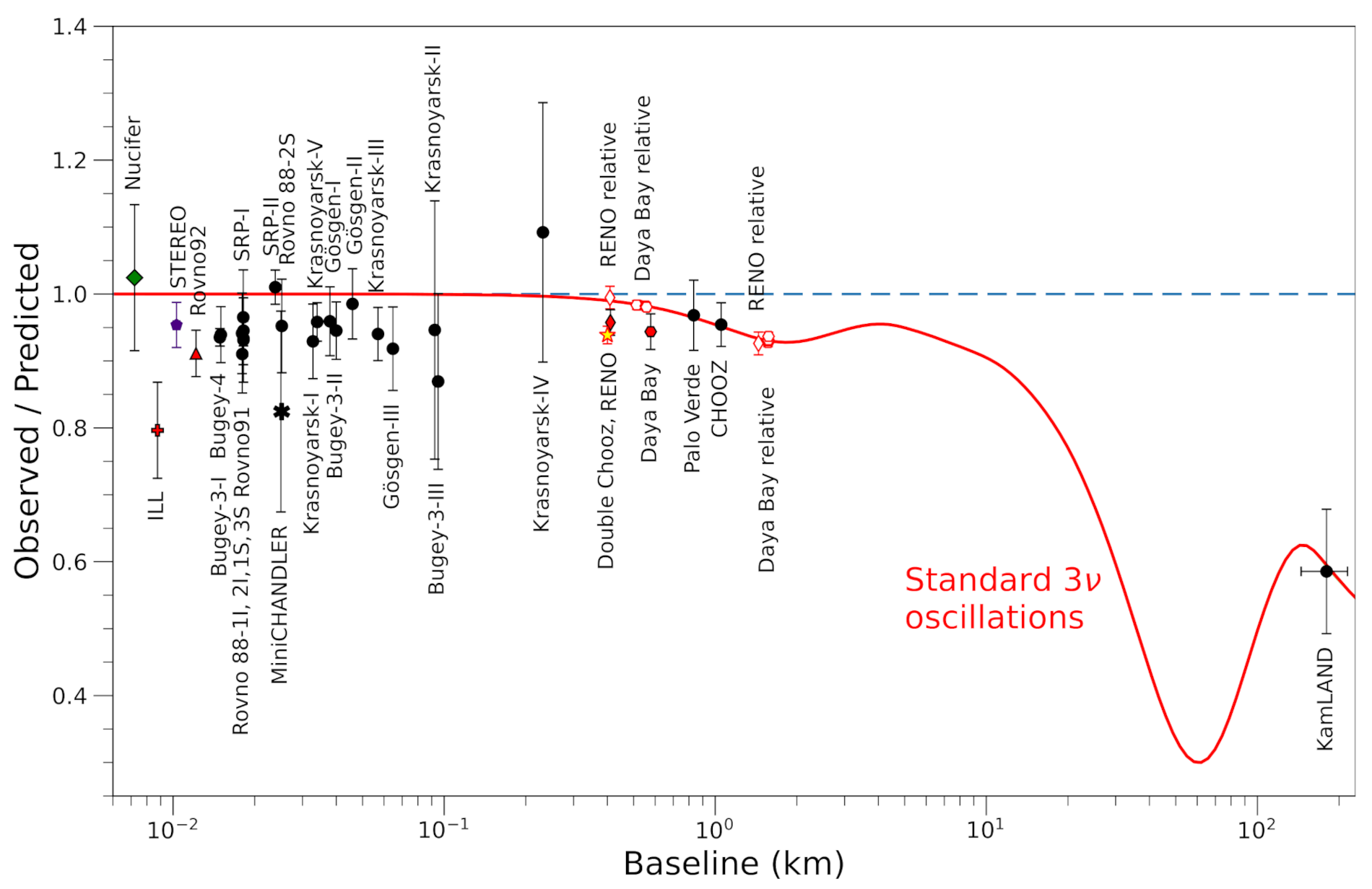
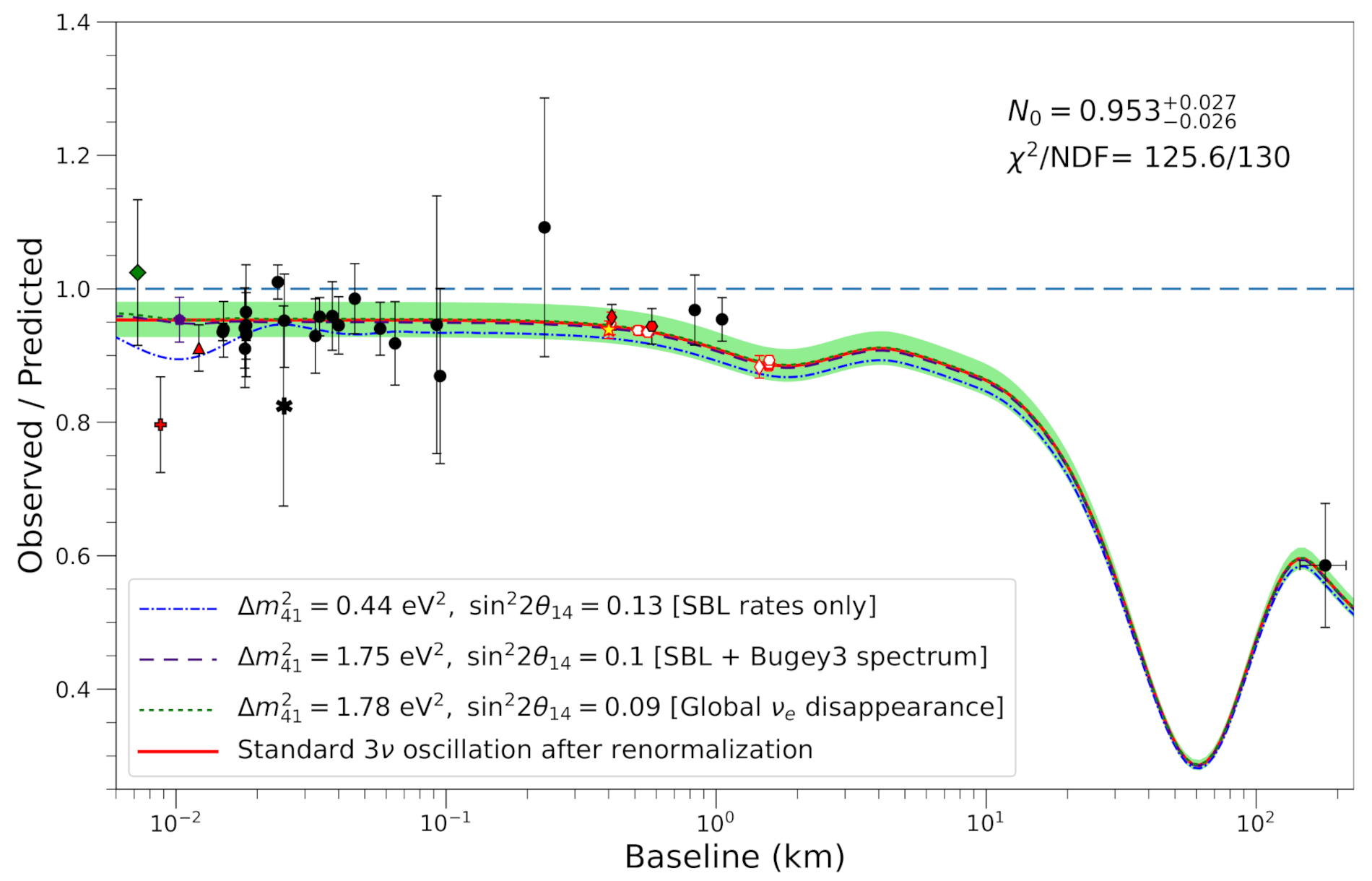
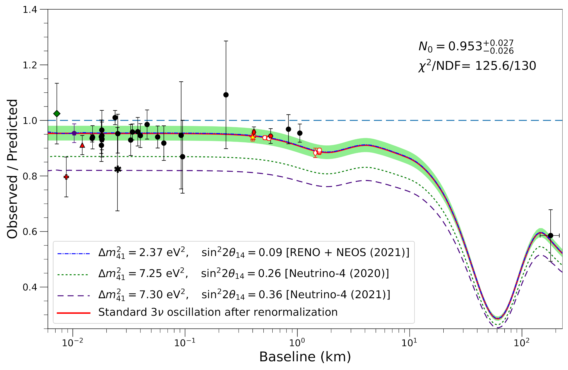
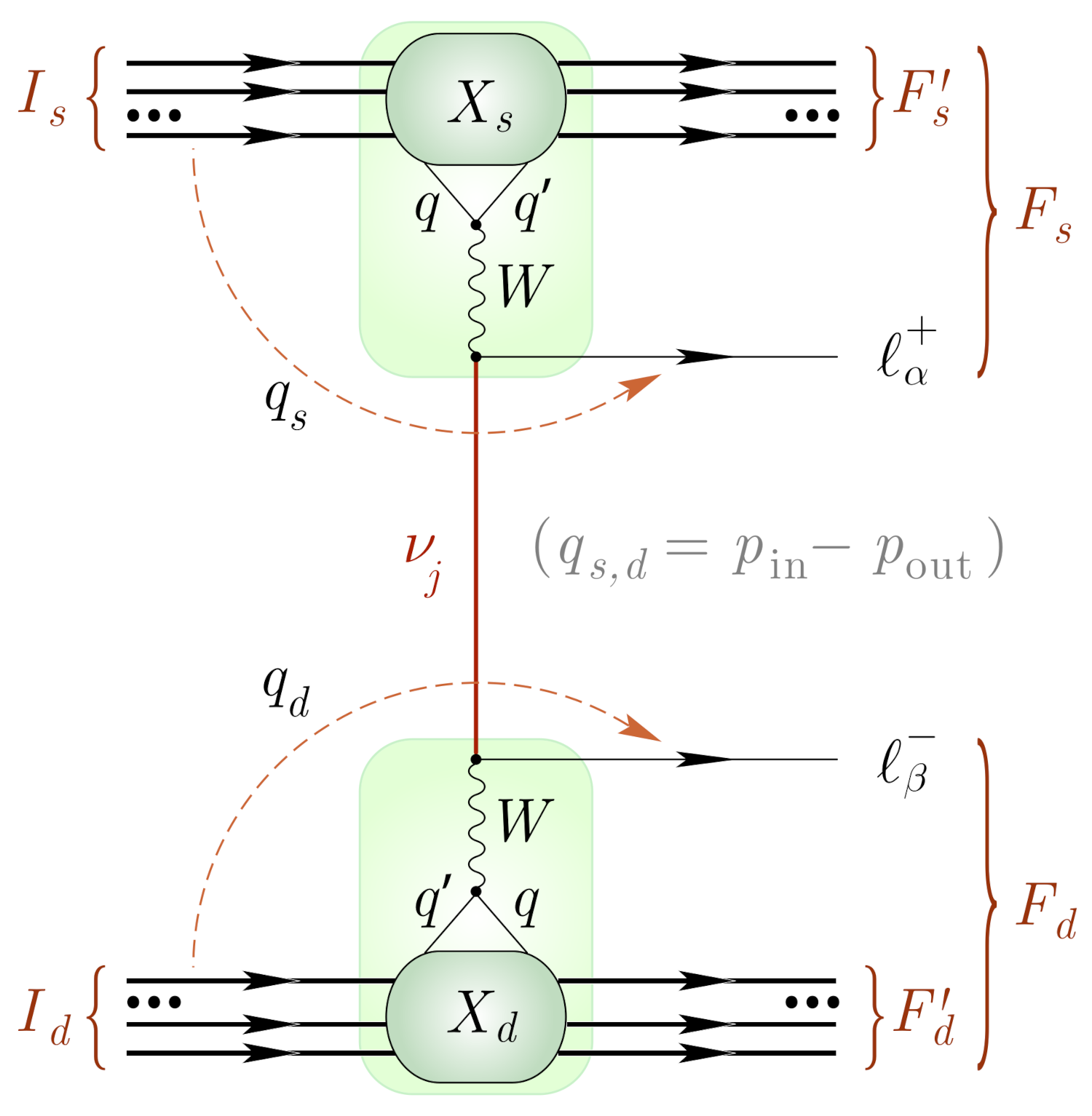
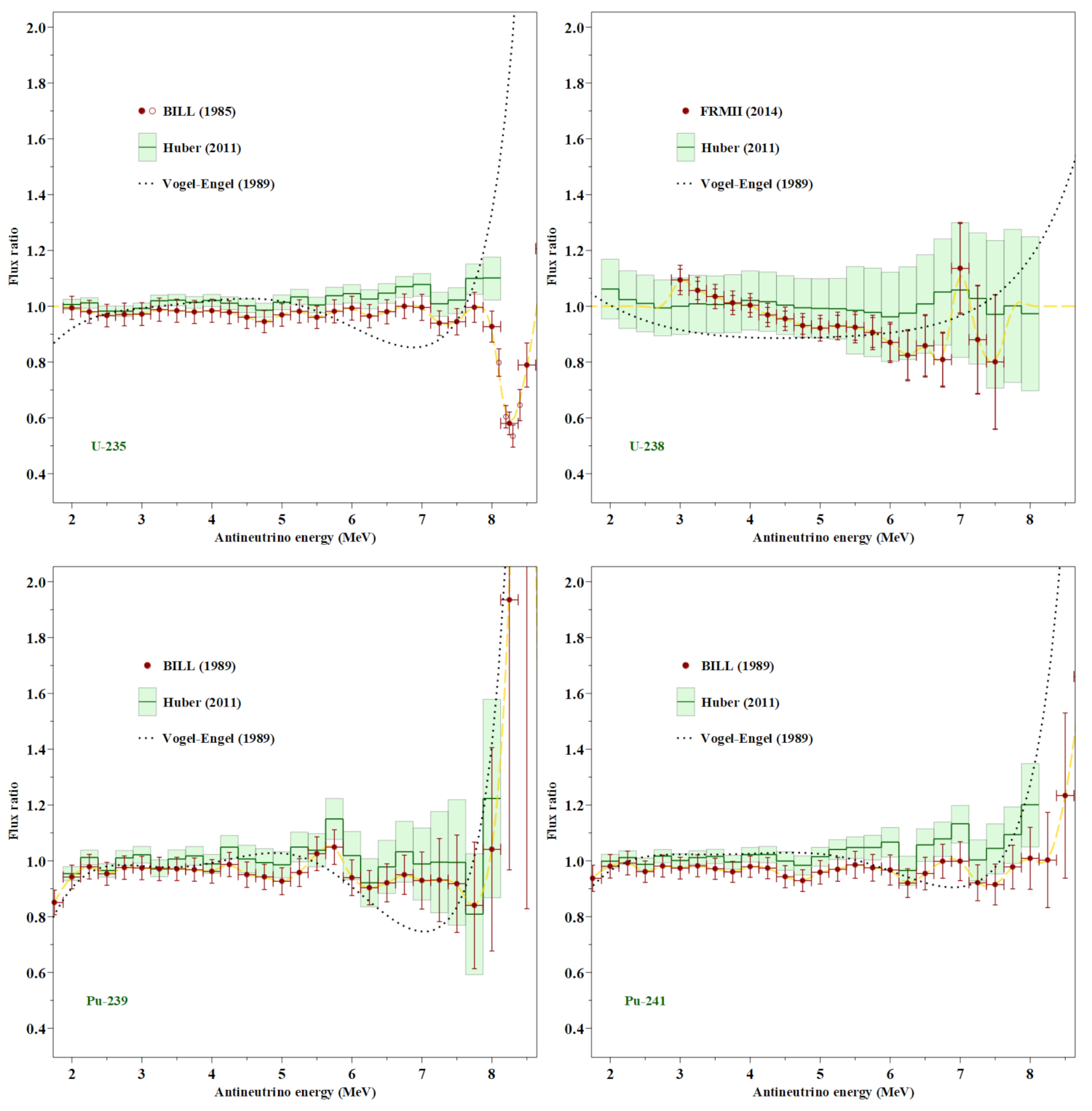
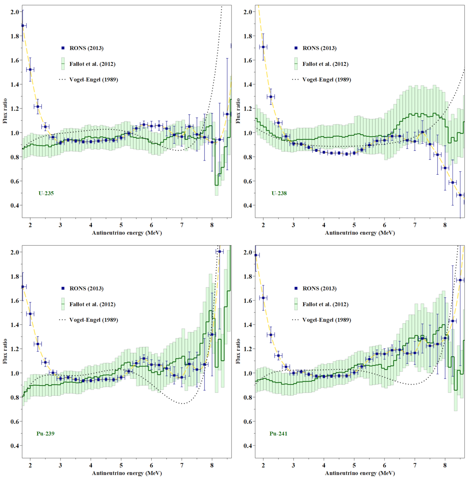
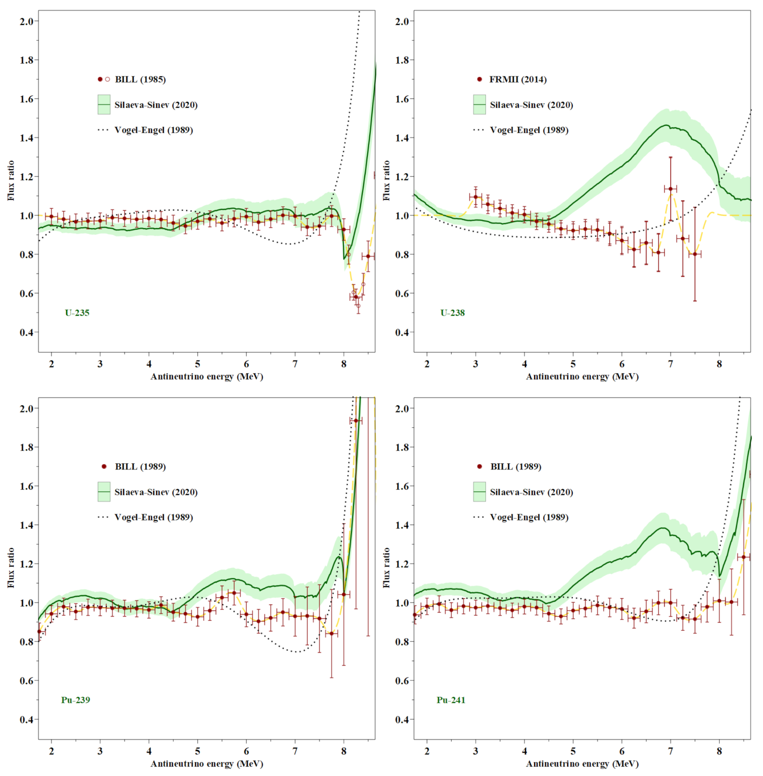
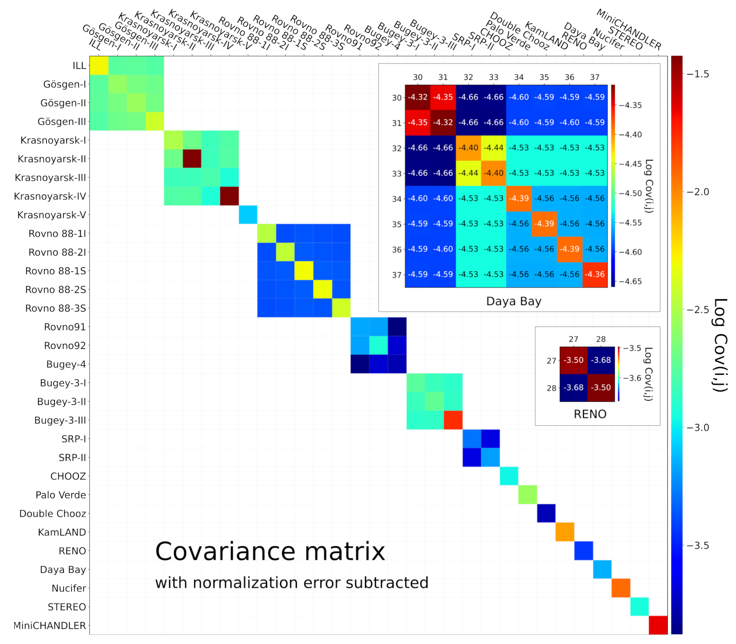
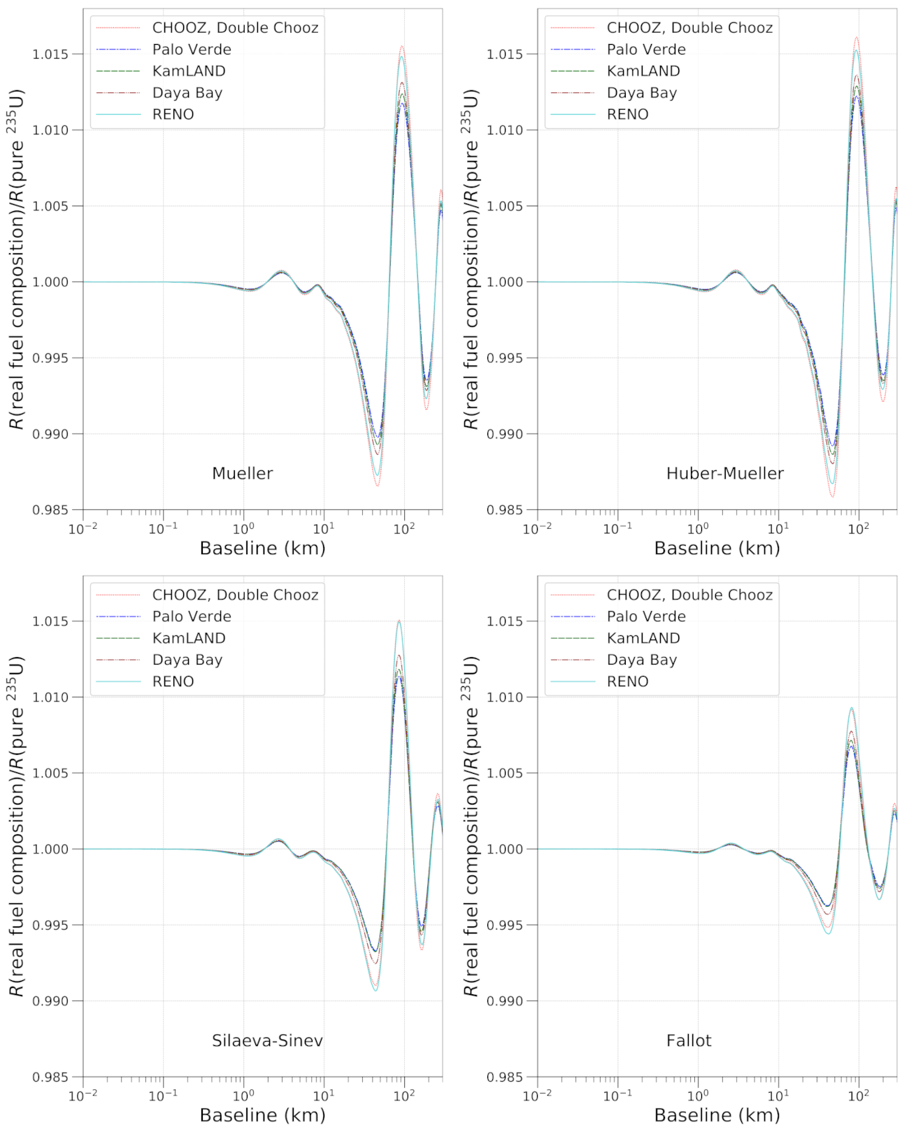
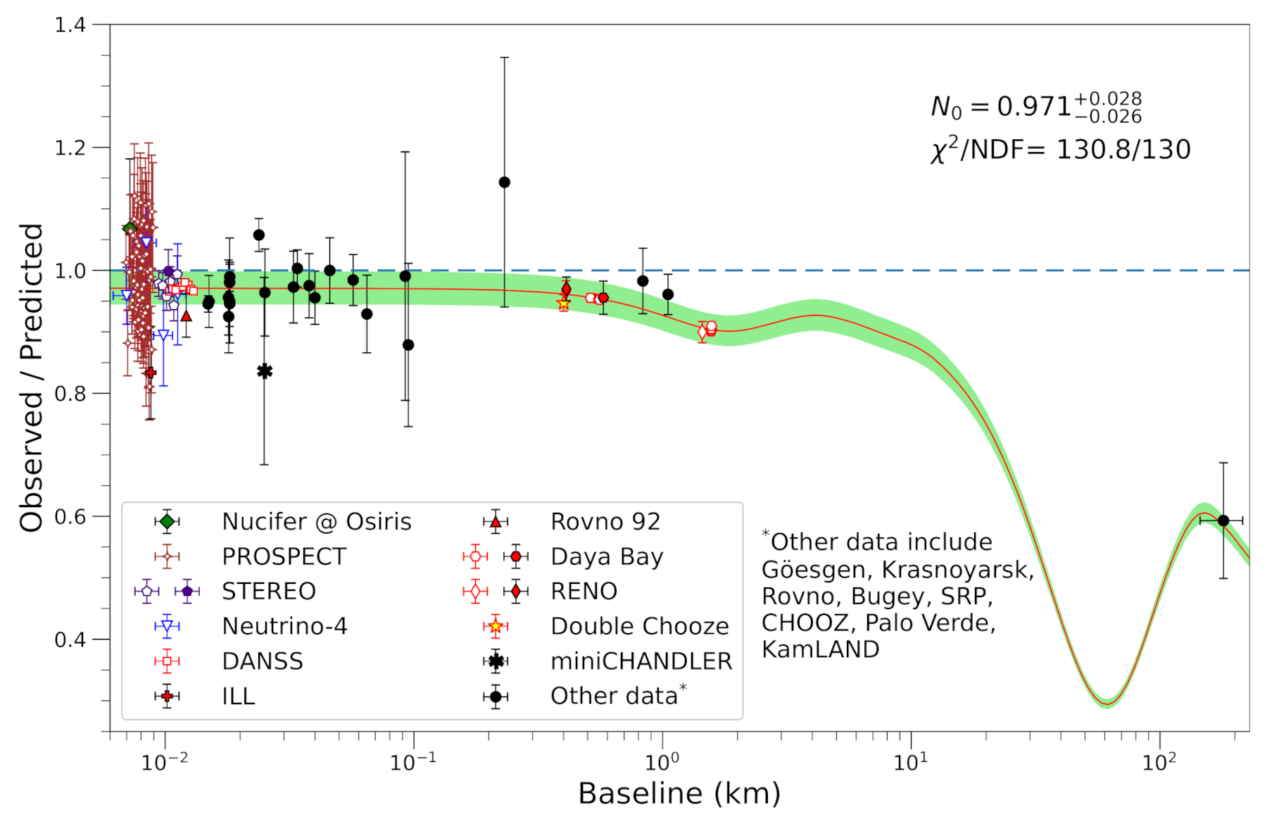
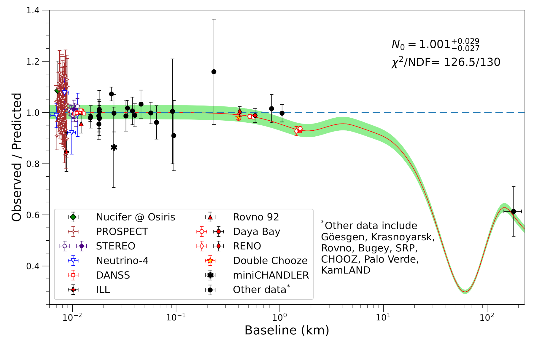
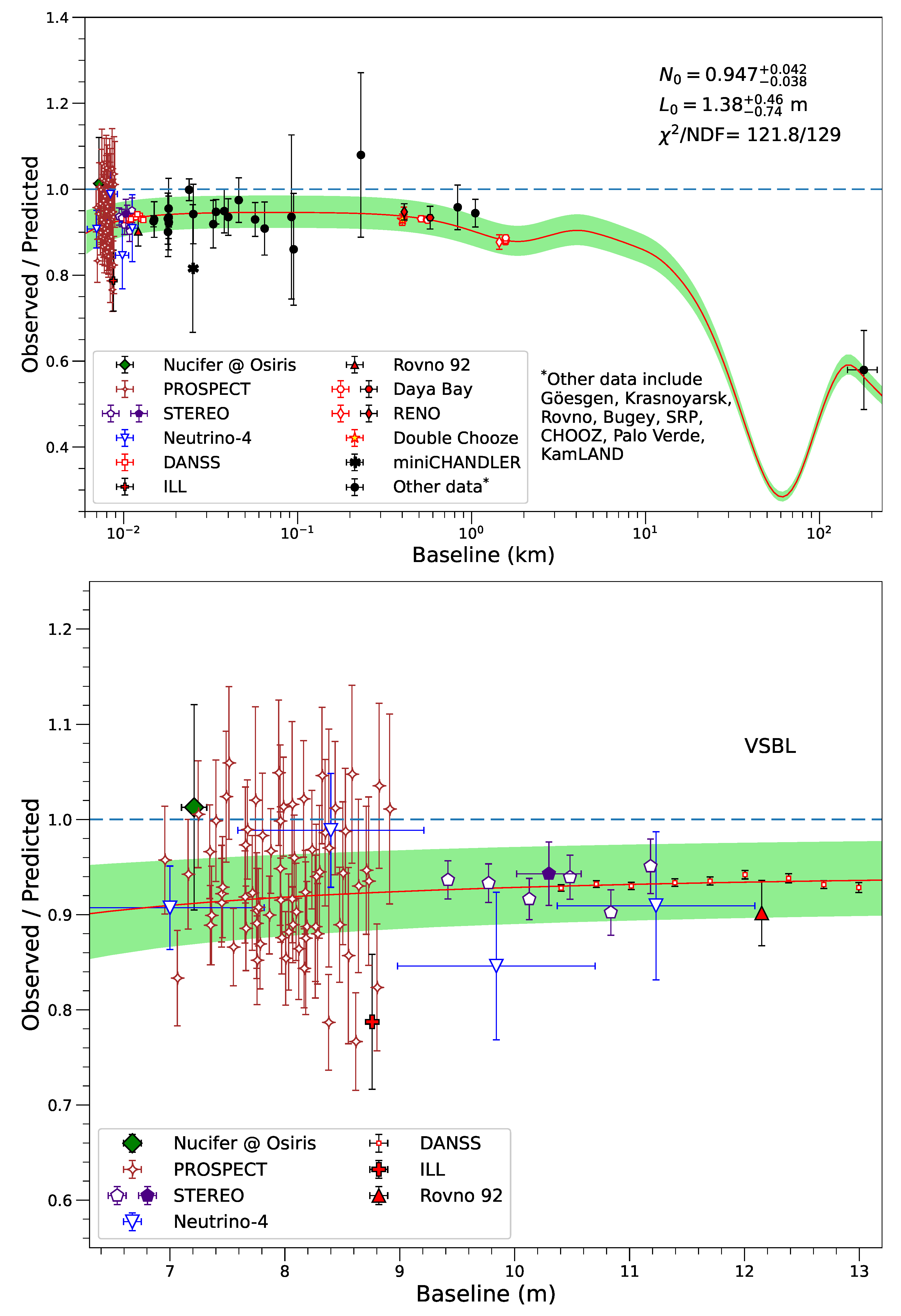
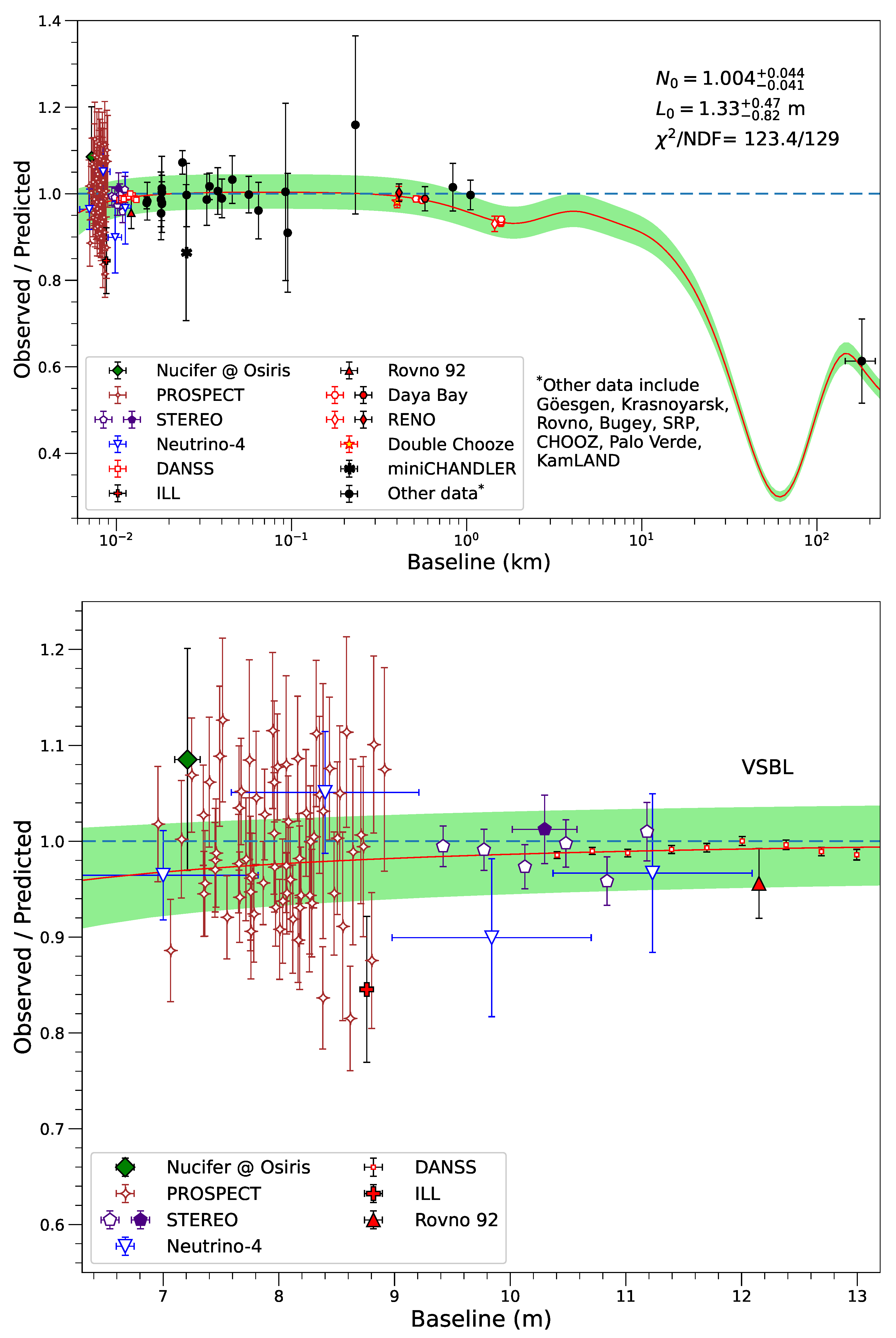
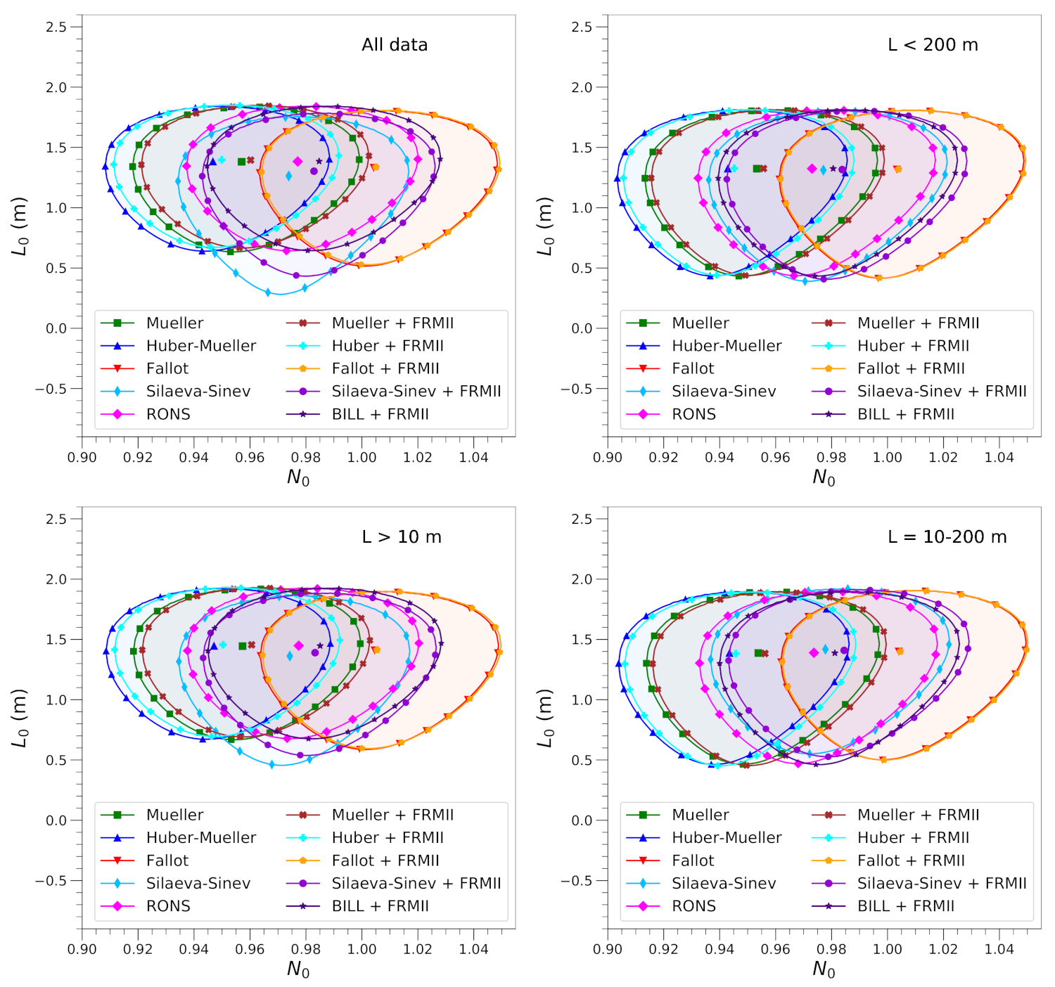
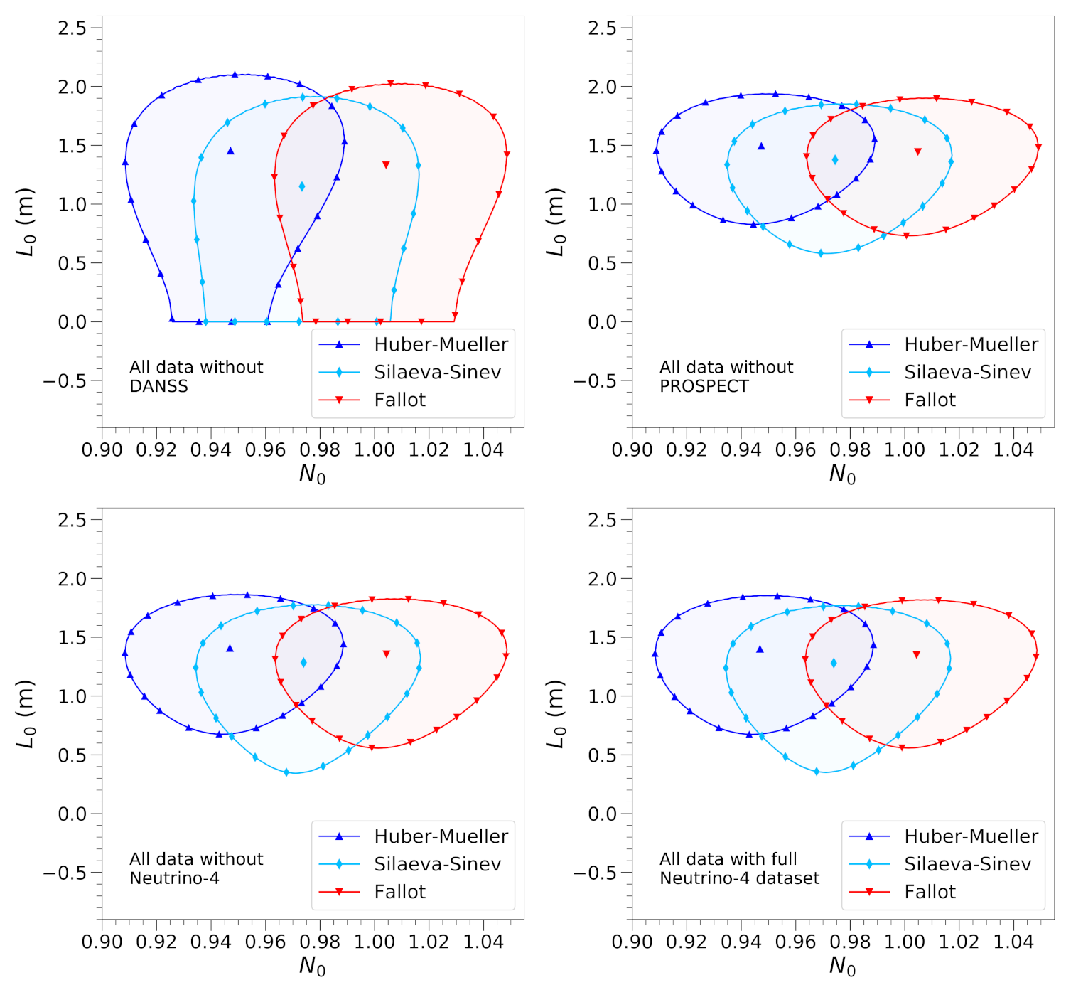
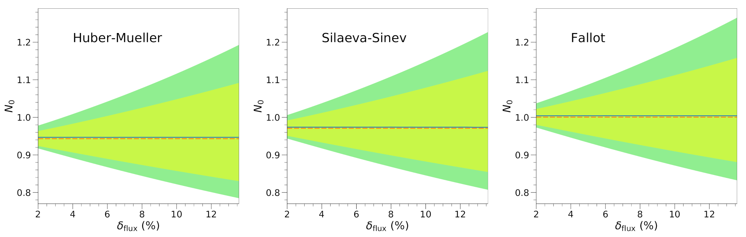
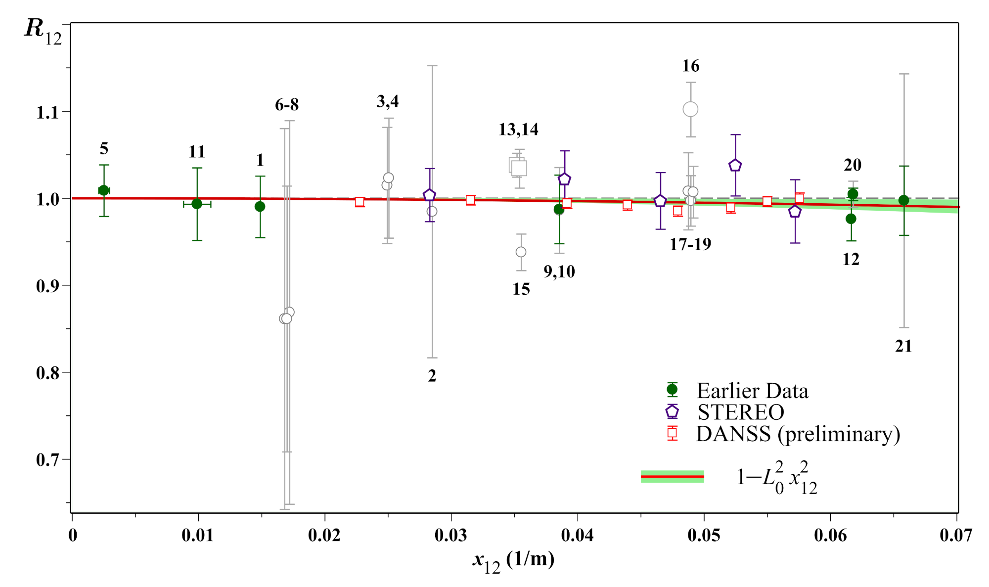
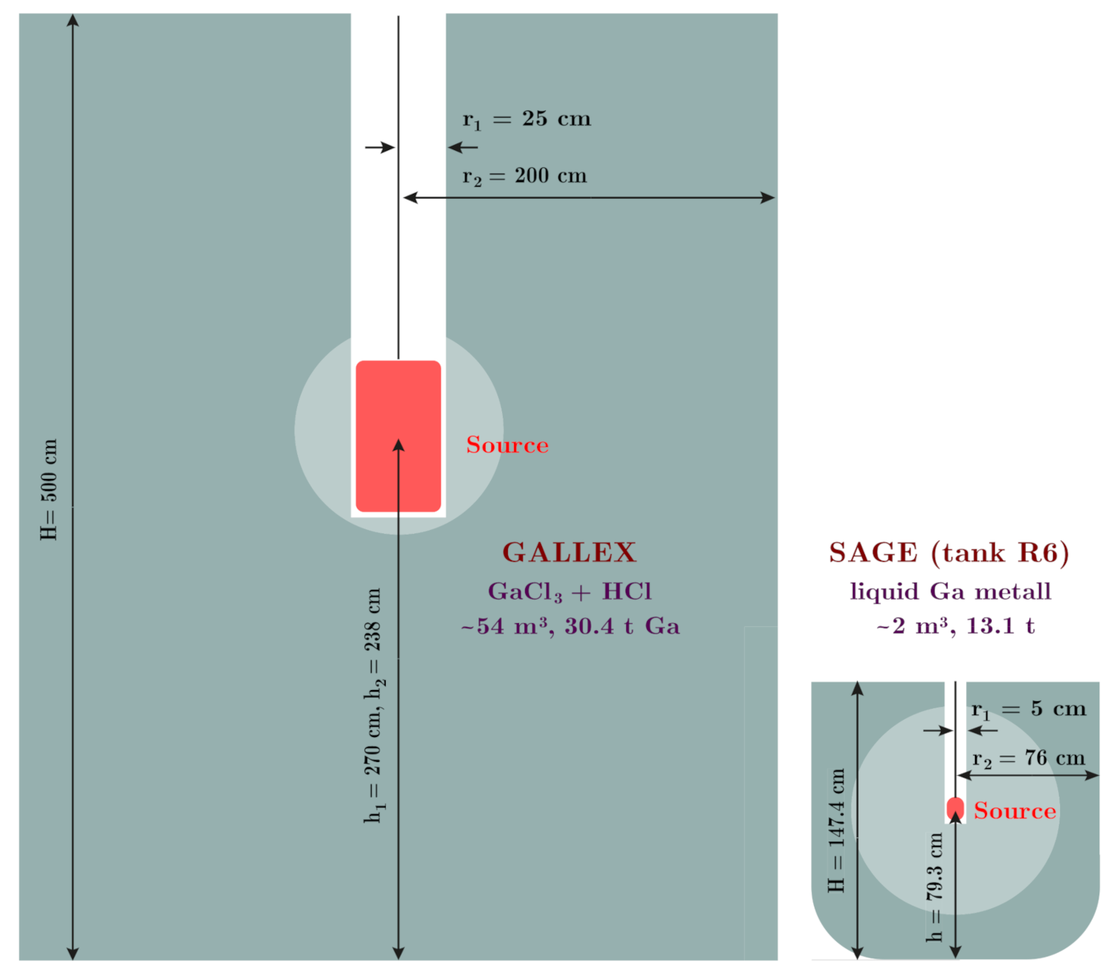
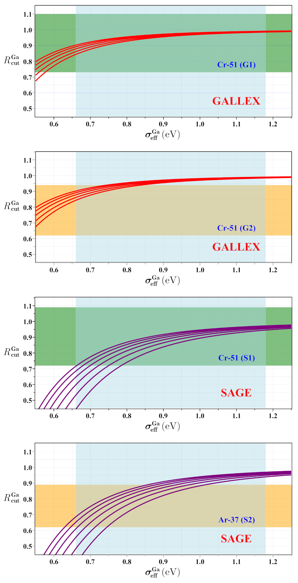
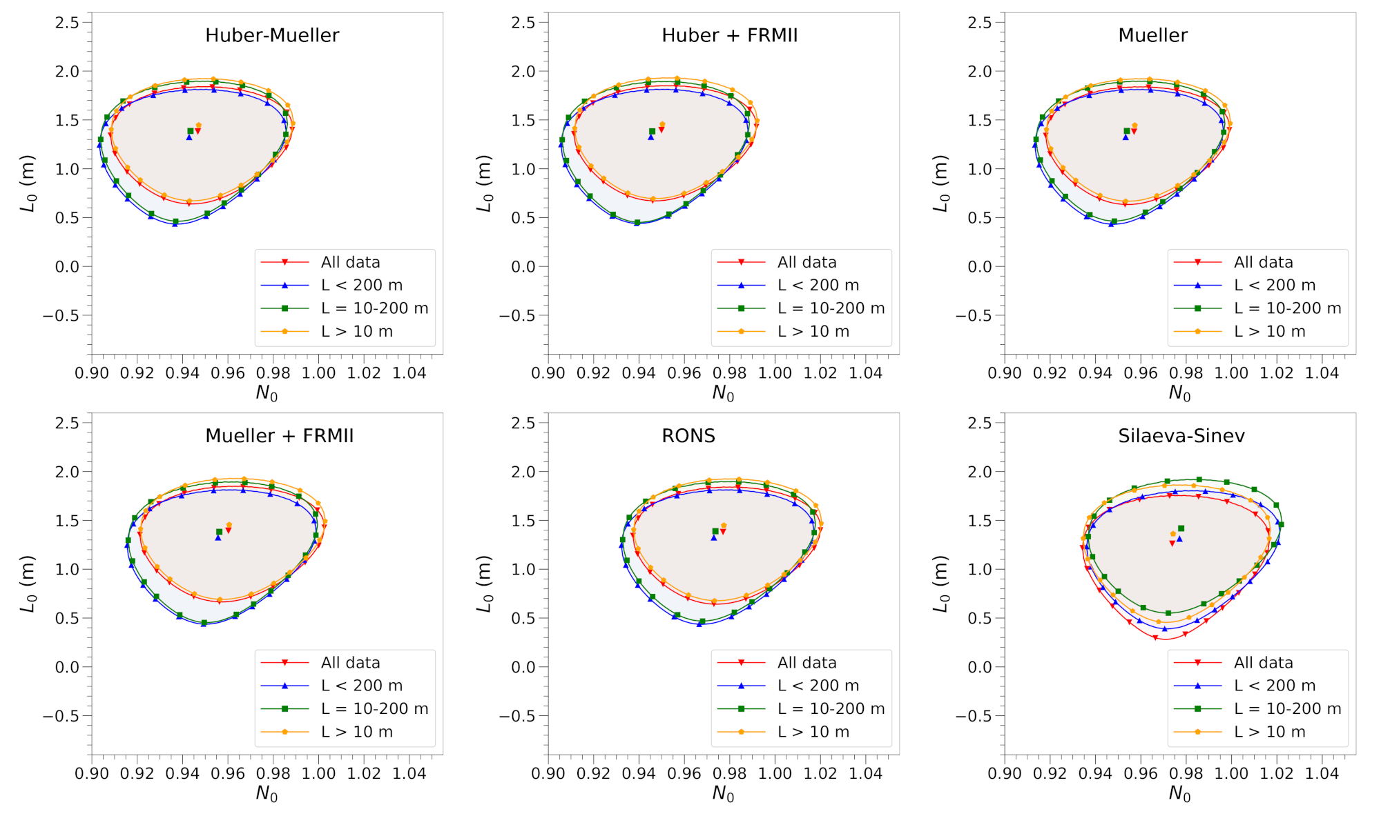
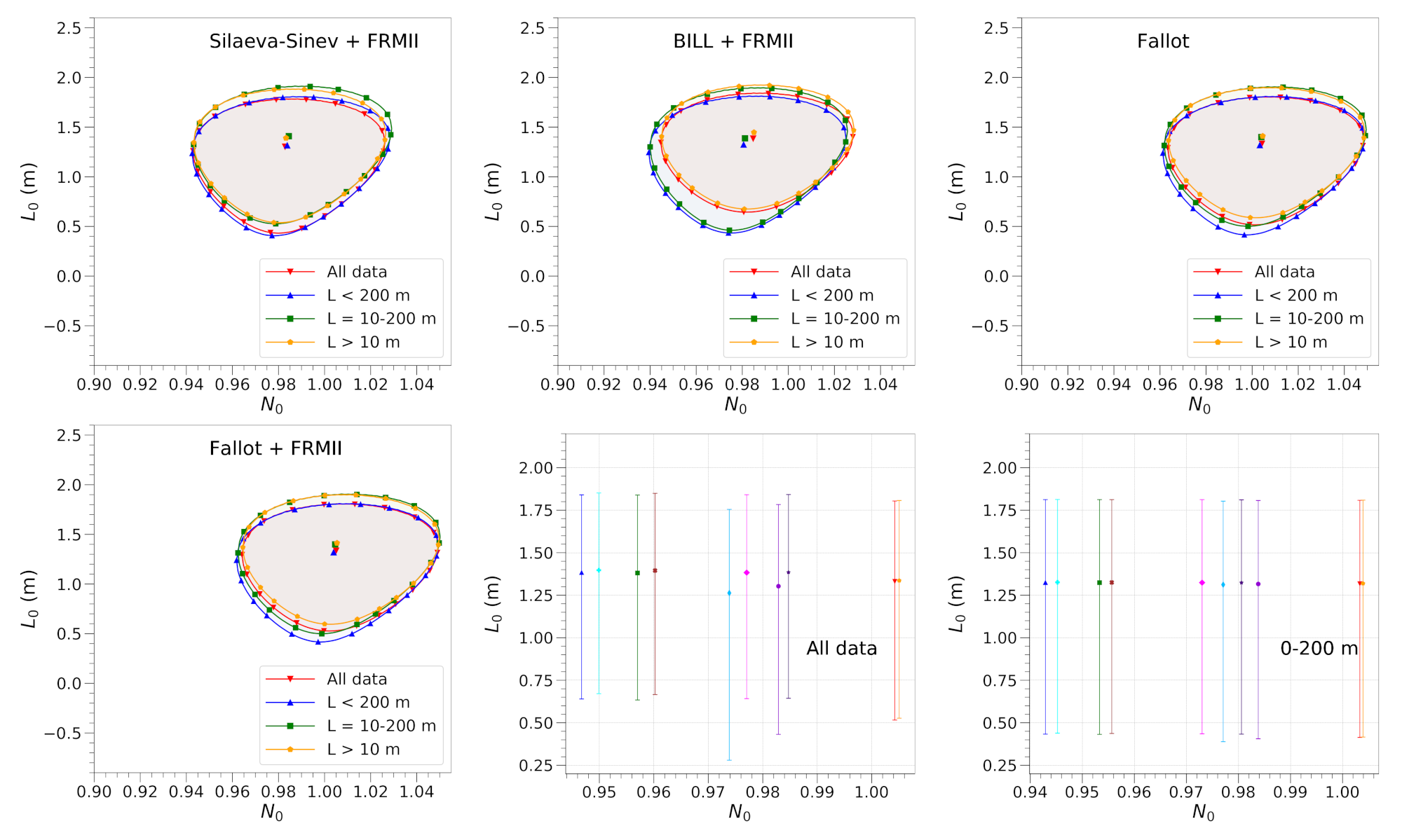
Table A1.
The main experimental dataset used in the subsequent analysis. The first column enumerates the experiments or (for segmented or movable detectors) baseline bins. The numbers in second column enumerate the groups of the cross-correlated measurements. The fractions of the main fissile isotopes are listed in columns 4–7. The ratios, R, of the observed to predicted integral production rates (used the analysis by Mention et al. [45] and corrected on updated neutron lifetime from [46]) are given in column 8. Columns 9–14 sequentially show the total experimental error, correlated error, baseline (or effective baseline), year of final publication or author’s communication, reference(s), and type of measurements (absolute or relative) for each experiment (bin). The overall uncertainty of the flux is subtracted from the systematic errors of all absolute data. Some correlation errors have been revised. The two special cases—groups 4 and 13—are described in Section 6.4 and the sub-matrices and are given by Equations (22) and (23). The results of the experiment DANSS (group 17) are preliminary (the data are kindly provided by the DANSS collaboration [200]). The data for groups 16, 18, and 19 were obtained by digitizing the measured dependencies of the counting rates (presented in arbitrary units) on distance L, divided by the approximations of these data. The block-diagonal covariance matrix for the experiment groups 1–10, 12, 14, 15, 20, and 21 (experiments/bins # 1–26, 29, 38, 39, 153, and 154) is shown in Figure 9, and the matrices for groups 11 and 13 (relative data) are shown as inserts.
| # | Gr. | Experiment | U | Pu | U | Pu | Ratio | (%) | (%) | L (m) | Year | Ref. | Type |
|---|---|---|---|---|---|---|---|---|---|---|---|---|---|
| 1 | 1 | ILL | 1.0 | 0 | 0 | 0 | 0.796 | 9.01 | 4.80 | 8.76 | 1981 | [7,8] | abs |
| 2 | 1 | Gösgen-I | 0.620 | 0.274 | 0.074 | 0.042 | 0.959 | 5.36 | 4.80 | 37.9 | 1986 | [16] | abs |
| 3 | 1 | Gösgen-II | 0.584 | 0.298 | 0.068 | 0.050 | 0.985 | 5.33 | 4.80 | 45.9 | 1986 | [16] | abs |
| 4 | 1 | Gösgen-III | 0.543 | 0.329 | 0.070 | 0.058 | 0.918 | 6.80 | 4.80 | 64.7 | 1986 | [16] | abs |
| 5 | 2 | Krasnoyarsk-I | 1.0 | 0 | 0 | 0 | 0.929 | 6.00 | 4.84 | 32.8 | 1987 | [17] | abs |
| 6 | 2 | Krasnoyarsk-II | 1.0 | 0 | 0 | 0 | 0.946 | 20.40 | 4.76 | 92.3 | 1987 | [17] | abs |
| 7 | 2 | Krasnoyarsk-III | 1.0 | 0 | 0 | 0 | 0.940 | 4.22 | 3.40 | 57.0 | 1994 | [19] | abs |
| 8 | 2 | Krasnoyarsk-IV | 1.0 | 0 | 0 | 0 | 1.092 | 17.75 | 3.40 | 231.4 | 1994 | [19] | abs |
| 9 | 2 | Krasnoyarsk-V | 1.0 | 0 | 0 | 0 | 0.958 | 3.00 | 0 | 34.0 | 1999 | [20] | abs |
| 10 | 3 | Rovno 88-1I | 0.607 | 0.277 | 0.074 | 0.042 | 0.910 | 6.39 | 2.20 | 18.00 | 1988 | [22] | abs |
| 11 | 3 | Rovno 88-2I | 0.603 | 0.276 | 0.076 | 0.045 | 0.941 | 6.39 | 2.20 | 17.96 | 1988 | [22] | abs |
| 12 | 3 | Rovno 88-1S | 0.606 | 0.277 | 0.074 | 0.043 | 0.965 | 7.34 | 2.20 | 18.15 | 1988 | [22] | abs |
| 13 | 3 | Rovno 88-2S | 0.557 | 0.313 | 0.076 | 0.054 | 0.952 | 7.34 | 2.20 | 25.17 | 1988 | [22] | abs |
| 14 | 3 | Rovno 88-3S | 0.606 | 0.274 | 0.074 | 0.046 | 0.931 | 6.77 | 2.20 | 18.18 | 1988 | [22] | abs |
| 15 | 4 | Rovno91 | 0.614 | 0.274 | 0.074 | 0.038 | 0.933 | 2.80 | 18.19 | 1991 | [24] | abs | |
| 16 | 4 | Rovno92 | 0.614 | 0.274 | 0.074 | 0.038 | 0.911 | 3.80 | 12.15 | 1992 | [26] | abs | |
| 17 | 4 | Bugey-4 | 0.538 | 0.328 | 0.078 | 0.056 | 0.935 | 1.40 | 14.88 | 1994 | [29] | abs | |
| 18 | 5 | Bugey-3-I | 0.538 | 0.328 | 0.078 | 0.056 | 0.939 | 4.45 | 4.00 | 15 | 1995 | [32] | abs |
| 19 | 5 | Bugey-3-II | 0.538 | 0.328 | 0.078 | 0.056 | 0.945 | 4.54 | 4.00 | 40 | 1995 | [32] | abs |
| 20 | 5 | Bugey-3-III | 0.538 | 0.328 | 0.078 | 0.056 | 0.869 | 15.10 | 4.00 | 95 | 1995 | [32] | abs |
| 21 | 6 | SRP-I | 1.0 | 0 | 0 | 0 | 0.945 | 2.40 | 1.50 | 18.18 | 1996 | [14] | abs |
| 22 | 6 | SRP-II | 1.0 | 0 | 0 | 0 | 1.010 | 2.53 | 1.50 | 23.82 | 1996 | [14] | abs |
| 23 | 7 | CHOOZ | 0.496 | 0.351 | 0.087 | 0.066 | 0.954 | 3.42 | – | 1052 | 2003 | [40] | abs |
| 24 | 8 | Palo Verde | 0.600 | 0.270 | 0.070 | 0.060 | 0.968 | 5.42 | – | 833.2 | 2001 | [36] | abs |
| 25 | 9 | Double Chooz | 0.520 | 0.333 | 0.087 | 0.060 | 0.939 | 1.40 | – | 400.3 | 2020 | [59] | abs |
| 26 | 10 | KamLAND | 0.571 | 0.295 | 0.078 | 0.056 | 0.586 | 15.87 | – | 180 | 2005 | [41] | abs |
| 27 | 11 | RENO | 0.556 | 0.326 | 0.071 | 0.047 | 0.999 | 1.78 | 1.50 | 409 | 2012 | [47] | rel |
| 28 | 11 | RENO | 0.556 | 0.326 | 0.071 | 0.047 | 0.930 | 1.92 | 1.50 | 1444 | 2012 | [47] | rel |
| 29 | 12 | RENO | 0.556 | 0.326 | 0.071 | 0.047 | 0.957 | 2.00 | – | 410.6 | 2020 | [49] | abs |
| 30 | 13 | Daya Bay | 0.564 | 0.303 | 0.076 | 0.056 | 0.995 | 0.70 | 517.78 | 2017 | [48] | rel | |
| 31 | 13 | Daya Bay | 0.564 | 0.303 | 0.076 | 0.056 | 0.995 | 0.70 | 513.05 | 2017 | [48] | rel | |
| 32 | 13 | Daya Bay | 0.564 | 0.303 | 0.076 | 0.056 | 0.994 | 0.63 | 554.39 | 2017 | [48] | rel | |
| 33 | 13 | Daya Bay | 0.564 | 0.303 | 0.076 | 0.056 | 0.992 | 0.64 | 557.80 | 2017 | [48] | rel | |
| 34 | 13 | Daya Bay | 0.564 | 0.303 | 0.076 | 0.056 | 0.938 | 0.68 | 1566.78 | 2017 | [48] | rel | |
| 35 | 13 | Daya Bay | 0.564 | 0.303 | 0.076 | 0.056 | 0.941 | 0.68 | 1569.13 | 2017 | [48] | rel | |
| 36 | 13 | Daya Bay | 0.564 | 0.303 | 0.076 | 0.056 | 0.942 | 0.68 | 1571.08 | 2017 | [48] | rel | |
| 37 | 13 | Daya Bay | 0.564 | 0.303 | 0.076 | 0.056 | 0.948 | 0.69 | 1572.93 | 2017 | [48] | rel | |
| 38 | 14 | Daya Bay | 0.564 | 0.304 | 0.076 | 0.056 | 0.944 | 2.83 | – | 578 | 2019 | [50] | abs |
| 39 | 15 | Nucifer | 0.926 | 0.061 | 0.008 | 0.005 | 1.024 | 10.65 | – | 7.21 | 2016 | [56] | abs |
| 40 | 16 | Neutrino-4 | 1.0 | 0 | 0 | 0 | 0.859 | 4.83 | 0 | 7.000 | 2020 | [88] | rel |
| 41 | 16 | Neutrino-4 | 1.0 | 0 | 0 | 0 | 0.936 | 6.05 | 0 | 8.400 | 2020 | [88] | rel |
| 42 | 16 | Neutrino-4 | 1.0 | 0 | 0 | 0 | 0.801 | 9.17 | 0 | 9.840 | 2020 | [88] | rel |
| 43 | 16 | Neutrino-4 | 1.0 | 0 | 0 | 0 | 0.861 | 8.56 | 0 | 11.230 | 2020 | [88] | rel |
| 44 | 16 | Neutrino-4 | 1.0 | 0 | 0 | 0 | 0.755 | 13.24 | 0 | 6.41 | 2020 | [88] | rel |
| 45 | 16 | Neutrino-4 | 1.0 | 0 | 0 | 0 | 0.717 | 14.23 | 0 | 6.64 | 2020 | [88] | rel |
| 46 | 16 | Neutrino-4 | 1.0 | 0 | 0 | 0 | 0.912 | 10.42 | 0 | 6.88 | 2020 | [88] | rel |
| 47 | 16 | Neutrino-4 | 1.0 | 0 | 0 | 0 | 0.700 | 14.29 | 0 | 7.11 | 2020 | [88] | rel |
| 48 | 16 | Neutrino-4 | 1.0 | 0 | 0 | 0 | 0.822 | 12.77 | 0 | 7.35 | 2020 | [88] | rel |
| 49 | 16 | Neutrino-4 | 1.0 | 0 | 0 | 0 | 0.913 | 13.14 | 0 | 7.58 | 2020 | [88] | rel |
| 50 | 16 | Neutrino-4 | 1.0 | 0 | 0 | 0 | 0.913 | 12.05 | 0 | 7.82 | 2020 | [88] | rel |
| 51 | 16 | Neutrino-4 | 1.0 | 0 | 0 | 0 | 0.900 | 12.78 | 0 | 8.06 | 2020 | [88] | rel |
| 52 | 16 | Neutrino-4 | 1.0 | 0 | 0 | 0 | 0.938 | 16.52 | 0 | 8.29 | 2020 | [88] | rel |
| 53 | 16 | Neutrino-4 | 1.0 | 0 | 0 | 0 | 0.812 | 20.32 | 0 | 8.53 | 2020 | [88] | rel |
| 54 | 16 | Neutrino-4 | 1.0 | 0 | 0 | 0 | 0.849 | 20.02 | 0 | 8.76 | 2020 | [88] | rel |
| 55 | 16 | Neutrino-4 | 1.0 | 0 | 0 | 0 | 0.681 | 26.43 | 0 | 9.00 | 2020 | [88] | rel |
| 56 | 16 | Neutrino-4 | 1.0 | 0 | 0 | 0 | 0.645 | 27.91 | 0 | 9.23 | 2020 | [88] | rel |
| 57 | 16 | Neutrino-4 | 1.0 | 0 | 0 | 0 | 0.672 | 29.02 | 0 | 9.47 | 2020 | [88] | rel |
| 58 | 16 | Neutrino-4 | 1.0 | 0 | 0 | 0 | 0.551 | 36.30 | 0 | 9.70 | 2020 | [88] | rel |
| 59 | 16 | Neutrino-4 | 1.0 | 0 | 0 | 0 | 0.780 | 26.28 | 0 | 9.94 | 2020 | [88] | rel |
| 60 | 16 | Neutrino-4 | 1.0 | 0 | 0 | 0 | 0.756 | 22.49 | 0 | 10.17 | 2020 | [88] | rel |
| 61 | 16 | Neutrino-4 | 1.0 | 0 | 0 | 0 | 0.973 | 16.44 | 0 | 10.41 | 2020 | [88] | rel |
| 62 | 16 | Neutrino-4 | 1.0 | 0 | 0 | 0 | 0.886 | 20.88 | 0 | 10.64 | 2020 | [88] | rel |
| 63 | 16 | Neutrino-4 | 1.0 | 0 | 0 | 0 | 0.352 | 62.50 | 0 | 10.88 | 2020 | [88] | rel |
| 64 | 16 | Neutrino-4 | 1.0 | 0 | 0 | 0 | 1.072 | 24.25 | 0 | 11.12 | 2020 | [88] | rel |
| 65 | 16 | Neutrino-4 | 1.0 | 0 | 0 | 0 | 0.727 | 39.89 | 0 | 11.35 | 2020 | [88] | rel |
| 66 | 16 | Neutrino-4 | 1.0 | 0 | 0 | 0 | 0.950 | 38.95 | 0 | 11.58 | 2020 | [88] | rel |
| 67 | 16 | Neutrino-4 | 1.0 | 0 | 0 | 0 | 1.246 | 32.91 | 0 | 11.82 | 2020 | [88] | rel |
| 68 | 17 | DANSS | 0.580 | 0.300 | 0.070 | 0.050 | 1.006 | 0.36 | 0 | 10.405 | 2020 | [200] | rel |
| 69 | 17 | DANSS | 0.580 | 0.300 | 0.070 | 0.050 | 1.012 | 0.43 | 0 | 11.395 | 2020 | [200] | rel |
| 70 | 17 | DANSS | 0.580 | 0.300 | 0.070 | 0.050 | 1.017 | 0.50 | 0 | 12.385 | 2020 | [200] | rel |
| 71 | 17 | DANSS | 0.580 | 0.300 | 0.070 | 0.050 | 1.010 | 0.38 | 0 | 10.710 | 2020 | [200] | rel |
| 72 | 17 | DANSS | 0.580 | 0.300 | 0.070 | 0.050 | 1.013 | 0.45 | 0 | 11.700 | 2020 | [200] | rel |
| 73 | 17 | DANSS | 0.580 | 0.300 | 0.070 | 0.050 | 1.009 | 0.44 | 0 | 12.690 | 2020 | [200] | rel |
| 74 | 17 | DANSS | 0.580 | 0.300 | 0.070 | 0.050 | 1.008 | 0.40 | 0 | 11.015 | 2020 | [200] | rel |
| 75 | 17 | DANSS | 0.580 | 0.300 | 0.070 | 0.050 | 1.021 | 0.47 | 0 | 12.005 | 2020 | [200] | rel |
| 76 | 17 | DANSS | 0.580 | 0.300 | 0.070 | 0.050 | 1.006 | 0.56 | 0 | 12.995 | 2020 | [200] | rel |
| 77 | 18 | PROSPECT | 0.990 | 0.003 | 0.003 | 0.003 | 0.994 | 5.92 | 0 | 6.955 | 2021 | [53] | rel |
| 78 | 18 | PROSPECT | 0.990 | 0.003 | 0.003 | 0.003 | 0.865 | 6.02 | 0 | 7.064 | 2021 | [53] | rel |
| 79 | 18 | PROSPECT | 0.990 | 0.003 | 0.003 | 0.003 | 0.978 | 6.11 | 0 | 7.158 | 2021 | [53] | rel |
| 80 | 18 | PROSPECT | 0.990 | 0.003 | 0.003 | 0.003 | 1.044 | 5.58 | 0 | 7.246 | 2021 | [53] | rel |
| 81 | 18 | PROSPECT | 0.990 | 0.003 | 0.003 | 0.003 | 1.003 | 5.10 | 0 | 7.346 | 2021 | [53] | rel |
| 82 | 18 | PROSPECT | 0.990 | 0.003 | 0.003 | 0.003 | 0.923 | 4.69 | 0 | 7.351 | 2021 | [53] | rel |
| 83 | 18 | PROSPECT | 0.990 | 0.003 | 0.003 | 0.003 | 0.933 | 5.77 | 0 | 7.361 | 2021 | [53] | rel |
| 84 | 18 | PROSPECT | 0.990 | 0.003 | 0.003 | 0.003 | 1.037 | 6.39 | 0 | 7.399 | 2021 | [53] | rel |
| 85 | 18 | PROSPECT | 0.990 | 0.003 | 0.003 | 0.003 | 0.947 | 5.10 | 0 | 7.448 | 2021 | [53] | rel |
| 86 | 18 | PROSPECT | 0.990 | 0.003 | 0.003 | 0.003 | 0.957 | 5.51 | 0 | 7.450 | 2021 | [53] | rel |
| 87 | 18 | PROSPECT | 0.990 | 0.003 | 0.003 | 0.003 | 0.964 | 5.72 | 0 | 7.457 | 2021 | [53] | rel |
| 88 | 18 | PROSPECT | 0.990 | 0.003 | 0.003 | 0.003 | 1.063 | 6.71 | 0 | 7.489 | 2021 | [53] | rel |
| 89 | 18 | PROSPECT | 0.990 | 0.003 | 0.003 | 0.003 | 1.100 | 7.58 | 0 | 7.513 | 2021 | [53] | rel |
| 90 | 18 | PROSPECT | 0.990 | 0.003 | 0.003 | 0.003 | 0.899 | 4.70 | 0 | 7.551 | 2021 | [53] | rel |
| 91 | 18 | PROSPECT | 0.990 | 0.003 | 0.003 | 0.003 | 0.954 | 5.26 | 0 | 7.652 | 2021 | [53] | rel |
| 92 | 18 | PROSPECT | 0.990 | 0.003 | 0.003 | 0.003 | 1.010 | 6.26 | 0 | 7.656 | 2021 | [53] | rel |
| 93 | 18 | PROSPECT | 0.990 | 0.003 | 0.003 | 0.003 | 0.919 | 5.01 | 0 | 7.661 | 2021 | [53] | rel |
| 94 | 18 | PROSPECT | 0.990 | 0.003 | 0.003 | 0.003 | 1.027 | 5.27 | 0 | 7.673 | 2021 | [53] | rel |
| 95 | 18 | PROSPECT | 0.990 | 0.003 | 0.003 | 0.003 | 0.958 | 6.54 | 0 | 7.715 | 2021 | [53] | rel |
| 96 | 18 | PROSPECT | 0.990 | 0.003 | 0.003 | 0.003 | 1.059 | 9.61 | 0 | 7.744 | 2021 | [53] | rel |
| 97 | 18 | PROSPECT | 0.990 | 0.003 | 0.003 | 0.003 | 0.925 | 6.50 | 0 | 7.754 | 2021 | [53] | rel |
| 98 | 18 | PROSPECT | 0.990 | 0.003 | 0.003 | 0.003 | 0.939 | 6.72 | 0 | 7.755 | 2021 | [53] | rel |
| 99 | 18 | PROSPECT | 0.990 | 0.003 | 0.003 | 0.003 | 0.885 | 5.48 | 0 | 7.758 | 2021 | [53] | rel |
| 100 | 18 | PROSPECT | 0.990 | 0.003 | 0.003 | 0.003 | 0.942 | 4.47 | 0 | 7.768 | 2021 | [53] | rel |
| 101 | 18 | PROSPECT | 0.990 | 0.003 | 0.003 | 0.003 | 0.902 | 5.43 | 0 | 7.783 | 2021 | [53] | rel |
| 102 | 18 | PROSPECT | 0.990 | 0.003 | 0.003 | 0.003 | 1.021 | 6.66 | 0 | 7.804 | 2021 | [53] | rel |
| 103 | 18 | PROSPECT | 0.990 | 0.003 | 0.003 | 0.003 | 0.934 | 4.55 | 0 | 7.865 | 2021 | [53] | rel |
| 104 | 18 | PROSPECT | 0.990 | 0.003 | 0.003 | 0.003 | 1.004 | 4.60 | 0 | 7.877 | 2021 | [53] | rel |
| 105 | 18 | PROSPECT | 0.990 | 0.003 | 0.003 | 0.003 | 1.089 | 7.29 | 0 | 7.946 | 2021 | [53] | rel |
| 106 | 18 | PROSPECT | 0.990 | 0.003 | 0.003 | 0.003 | 0.984 | 6.29 | 0 | 7.958 | 2021 | [53] | rel |
| 107 | 18 | PROSPECT | 0.990 | 0.003 | 0.003 | 0.003 | 1.036 | 8.01 | 0 | 7.959 | 2021 | [53] | rel |
| 108 | 18 | PROSPECT | 0.990 | 0.003 | 0.003 | 0.003 | 0.950 | 4.84 | 0 | 7.962 | 2021 | [53] | rel |
| 109 | 18 | PROSPECT | 0.990 | 0.003 | 0.003 | 0.003 | 0.909 | 4.35 | 0 | 7.972 | 2021 | [53] | rel |
| 110 | 18 | PROSPECT | 0.990 | 0.003 | 0.003 | 0.003 | 1.052 | 5.14 | 0 | 7.987 | 2021 | [53] | rel |
| 111 | 18 | PROSPECT | 0.990 | 0.003 | 0.003 | 0.003 | 0.887 | 5.75 | 0 | 8.007 | 2021 | [53] | rel |
| 112 | 18 | PROSPECT | 0.990 | 0.003 | 0.003 | 0.003 | 0.915 | 6.92 | 0 | 8.032 | 2021 | [53] | rel |
| 113 | 18 | PROSPECT | 0.990 | 0.003 | 0.003 | 0.003 | 0.951 | 5.02 | 0 | 8.062 | 2021 | [53] | rel |
| 114 | 18 | PROSPECT | 0.990 | 0.003 | 0.003 | 0.003 | 1.055 | 8.56 | 0 | 8.063 | 2021 | [53] | rel |
| 115 | 18 | PROSPECT | 0.990 | 0.003 | 0.003 | 0.003 | 0.923 | 4.49 | 0 | 8.068 | 2021 | [53] | rel |
| 116 | 18 | PROSPECT | 0.990 | 0.003 | 0.003 | 0.003 | 0.996 | 4.69 | 0 | 8.081 | 2021 | [53] | rel |
| 117 | 18 | PROSPECT | 0.990 | 0.003 | 0.003 | 0.003 | 0.937 | 5.67 | 0 | 8.098 | 2021 | [53] | rel |
| 118 | 18 | PROSPECT | 0.990 | 0.003 | 0.003 | 0.003 | 0.897 | 6.16 | 0 | 8.120 | 2021 | [53] | rel |
| 119 | 18 | PROSPECT | 0.990 | 0.003 | 0.003 | 0.003 | 1.061 | 6.00 | 0 | 8.162 | 2021 | [53] | rel |
| 120 | 18 | PROSPECT | 0.990 | 0.003 | 0.003 | 0.003 | 0.876 | 4.92 | 0 | 8.167 | 2021 | [53] | rel |
| 121 | 18 | PROSPECT | 0.990 | 0.003 | 0.003 | 0.003 | 0.959 | 4.77 | 0 | 8.176 | 2021 | [53] | rel |
| 122 | 18 | PROSPECT | 0.990 | 0.003 | 0.003 | 0.003 | 0.909 | 9.16 | 0 | 8.181 | 2021 | [53] | rel |
| 123 | 18 | PROSPECT | 0.990 | 0.003 | 0.003 | 0.003 | 0.921 | 5.35 | 0 | 8.190 | 2021 | [53] | rel |
| 124 | 18 | PROSPECT | 0.990 | 0.003 | 0.003 | 0.003 | 1.005 | 6.43 | 0 | 8.235 | 2021 | [53] | rel |
| 125 | 18 | PROSPECT | 0.990 | 0.003 | 0.003 | 0.003 | 0.921 | 8.46 | 0 | 8.265 | 2021 | [53] | rel |
| 126 | 18 | PROSPECT | 0.990 | 0.003 | 0.003 | 0.003 | 0.921 | 6.49 | 0 | 8.266 | 2021 | [53] | rel |
| 127 | 18 | PROSPECT | 0.990 | 0.003 | 0.003 | 0.003 | 0.976 | 5.85 | 0 | 8.273 | 2021 | [53] | rel |
| 128 | 18 | PROSPECT | 0.990 | 0.003 | 0.003 | 0.003 | 0.913 | 6.00 | 0 | 8.284 | 2021 | [53] | rel |
| 129 | 18 | PROSPECT | 0.990 | 0.003 | 0.003 | 0.003 | 0.981 | 7.38 | 0 | 8.301 | 2021 | [53] | rel |
| 130 | 18 | PROSPECT | 0.990 | 0.003 | 0.003 | 0.003 | 1.086 | 6.85 | 0 | 8.323 | 2021 | [53] | rel |
| 131 | 18 | PROSPECT | 0.990 | 0.003 | 0.003 | 0.003 | 1.024 | 7.81 | 0 | 8.350 | 2021 | [53] | rel |
| 132 | 18 | PROSPECT | 0.990 | 0.003 | 0.003 | 0.003 | 0.817 | 6.39 | 0 | 8.380 | 2021 | [53] | rel |
| 133 | 18 | PROSPECT | 0.990 | 0.003 | 0.003 | 0.003 | 1.007 | 12.88 | 0 | 8.382 | 2021 | [53] | rel |
| 134 | 18 | PROSPECT | 0.990 | 0.003 | 0.003 | 0.003 | 1.050 | 6.93 | 0 | 8.437 | 2021 | [53] | rel |
| 135 | 18 | PROSPECT | 0.990 | 0.003 | 0.003 | 0.003 | 0.923 | 6.80 | 0 | 8.477 | 2021 | [53] | rel |
| 136 | 18 | PROSPECT | 0.990 | 0.003 | 0.003 | 0.003 | 0.980 | 7.95 | 0 | 8.505 | 2021 | [53] | rel |
| 137 | 18 | PROSPECT | 0.990 | 0.003 | 0.003 | 0.003 | 1.025 | 6.70 | 0 | 8.526 | 2021 | [53] | rel |
| 138 | 18 | PROSPECT | 0.990 | 0.003 | 0.003 | 0.003 | 0.890 | 10.80 | 0 | 8.552 | 2021 | [53] | rel |
| 139 | 18 | PROSPECT | 0.990 | 0.003 | 0.003 | 0.003 | 1.087 | 8.92 | 0 | 8.584 | 2021 | [53] | rel |
| 140 | 18 | PROSPECT | 0.990 | 0.003 | 0.003 | 0.003 | 0.796 | 6.69 | 0 | 8.616 | 2021 | [53] | rel |
| 141 | 18 | PROSPECT | 0.990 | 0.003 | 0.003 | 0.003 | 0.965 | 9.79 | 0 | 8.640 | 2021 | [53] | rel |
| 142 | 18 | PROSPECT | 0.990 | 0.003 | 0.003 | 0.003 | 0.983 | 7.11 | 0 | 8.708 | 2021 | [53] | rel |
| 143 | 18 | PROSPECT | 0.990 | 0.003 | 0.003 | 0.003 | 0.971 | 9.46 | 0 | 8.729 | 2021 | [53] | rel |
| 144 | 18 | PROSPECT | 0.990 | 0.003 | 0.003 | 0.003 | 0.855 | 8.10 | 0 | 8.802 | 2021 | [53] | rel |
| 145 | 18 | PROSPECT | 0.990 | 0.003 | 0.003 | 0.003 | 1.075 | 8.38 | 0 | 8.820 | 2021 | [53] | rel |
| 146 | 18 | PROSPECT | 0.990 | 0.003 | 0.003 | 0.003 | 1.050 | 9.87 | 0 | 8.912 | 2021 | [53] | rel |
| 147 | 19 | STEREO | 1.0 | 0 | 0 | 0 | 1.015 | 2.13 | 0 | 9.42 | 2020 | [51] | rel |
| 148 | 19 | STEREO | 1.0 | 0 | 0 | 0 | 1.011 | 2.17 | 0 | 9.77 | 2020 | [51] | rel |
| 149 | 19 | STEREO | 1.0 | 0 | 0 | 0 | 0.993 | 2.37 | 0 | 10.13 | 2020 | [51] | rel |
| 150 | 19 | STEREO | 1.0 | 0 | 0 | 0 | 1.018 | 2.48 | 0 | 10.48 | 2020 | [51] | rel |
| 151 | 19 | STEREO | 1.0 | 0 | 0 | 0 | 0.978 | 2.64 | 0 | 10.84 | 2020 | [51] | rel |
| 152 | 19 | STEREO | 1.0 | 0 | 0 | 0 | 1.031 | 3.02 | 0 | 11.18 | 2020 | [51] | rel |
| 153 | 20 | STEREO | 1.0 | 0 | 0 | 0 | 0.954 | 3.53 | – | 10.3 | 2020 | [57] | abs |
| 154 | 21 | MiniCHANDLER | 0.580 | 0.300 | 0.070 | 0.050 | 0.824 | 18.20 | – | 25 | 2020 | [58] | abs |
Table A2.
Solid-angle corrected ratios () of the IBD events measured at two distances (, ) from reactor core by using movable or identical detectors. Some data are recalculated from the originally published inverse ratios (), event number or cross section ratios. Subscript “ det+react” means that the error includes statistics, uncertainty associated with the detection efficiency, and insufficient knowledge of the reactor power. Data marked with tick (√) are used in the global statistical analysis. The rest data are not involved because they are either not independent, or have already been included in a different form, or are out of date. All the data, except those marked with an asterisk (*), are shown in Figure 20. The earlier measurements with high energy thresholds (e.g. [10]) are not included. We show, for contrast, obviously outdated data from experiments with the Irvine mobile neutrino oscillation detector in the SRP Neutrino Laboratory [12,13] and with the movable Bugey detector [27].
| # | Experiment | Year | Ref. | (m) | (m) | Comment | ||
|---|---|---|---|---|---|---|---|---|
| 1 | Gösgen | 1984 | [15] | from inverse ratio | √ | |||
| 2 | Krasnoyarsk | 1987 | [17] | from event number ratio | ||||
| from cross section ratio | * | |||||||
| 3 | Krasnoyarsk | 1990 | [18] | from cross section ratio | ||||
| 4 | from cross section ratio | |||||||
| 5 | from event number ratio | √ | ||||||
| from cross section ratio | * | |||||||
| 6 | from event number ratio | |||||||
| 7 | from event number ratio | |||||||
| 8 | Krasnoyarsk | 1994 | [19] | from event number ratio | ||||
| 9 | Rovno | 1986 | [21] | 18 | 25 | |||
| 10 | Rovno | 1988 | [22] | 18 | 25 | from inverse ratio | √ | |
| 11 | Rovno | 1991 | [24] | from cross section ratio | √ | |||
| 12 | Rovno | 1992 | [26] | √ | ||||
| 13 | SRP | 1986 | [12] | |||||
| 14 | SRP | 1987 | [13] | |||||
| 15 | SRP | 1996 | [14] | from event number ratio | ||||
| 16 | Bugey | 1984 | [27] | |||||
| 17 | Bugey | 1988 | [30] | integrated spectra | ||||
| 18 | standard shielding data | |||||||
| 19 | data with lowest threshold | |||||||
| 20 | Bugey | 1995 | [32] | 15 | 40 | from inverse spectrum ratio | √ | |
| from double ratio | * | |||||||
| 21 | 15 | 95 | from inverse spectrum ratio | √ | ||||
| from double ratio | * |
Appendix B. Results of Statistical Analysis
Table A3.
A summary of the results of one- and two-parameter fits performed for different data subsets and spectrum models; p is the right-tail p-value, is the relative change (in percent) of the NDF values for each pair of these fits, and is the roughly estimated number of standard deviations of from zero.
| One-Parameter Fit | Two-Parameter Fit | ||||||||
|---|---|---|---|---|---|---|---|---|---|
| (m) | (%) | ||||||||
| 1. All data, NDF = 130 for one- and 129 for two-parameter fit | |||||||||
| Mueller | |||||||||
| Mueller + FRMII | |||||||||
| Huber–Mueller | |||||||||
| Huber + FRMII | |||||||||
| Fallot | |||||||||
| Fallot + FRMII | |||||||||
| Silaeva–Sinev | |||||||||
| Silaeva–Sinev + FRMII | |||||||||
| RONS | |||||||||
| BILL + FRMII | |||||||||
| 2. m, NDF = 54 for one- and 53 for two-parameter fit | |||||||||
| Mueller | |||||||||
| Mueller + FRMII | |||||||||
| Huber–Mueller | |||||||||
| Huber + FRMII | |||||||||
| Fallot | |||||||||
| Fallot + FRMII | |||||||||
| Silaeva–Sinev | |||||||||
| Silaeva–Sinev + FRMII | |||||||||
| RONS | |||||||||
| BILL + FRMII | |||||||||
| 3. m, NDF = 115 for one- and 114 for two-parameter fit | |||||||||
| Mueller | |||||||||
| Mueller + FRMII | |||||||||
| Huber–Mueller | |||||||||
| Huber + FRMII | |||||||||
| Fallot | |||||||||
| Fallot + FRMII | |||||||||
| Silaeva–Sinev | |||||||||
| Silaeva–Sinev + FRMII | |||||||||
| RONS | |||||||||
| BILL + FRMII | |||||||||
| 4. m, NDF = 39 for one- and 38 for two-parameter fit | |||||||||
| Mueller | |||||||||
| Mueller + FRMII | |||||||||
| Huber–Mueller | |||||||||
| Huber + FRMII | |||||||||
| Fallot | |||||||||
| Fallot + FRMII | |||||||||
| Silaeva–Sinev | |||||||||
| Silaeva–Sinev + FRMII | |||||||||
| RONS | |||||||||
| BILL + FRMII | |||||||||
| 5. All data without DANSS, NDF = 122 for one- and 121 for two-parameter fit | |||||||||
| Mueller | |||||||||
| Mueller + FRMII | |||||||||
| Huber–Mueller | |||||||||
| Huber + FRMII | |||||||||
| Fallot | |||||||||
| Fallot + FRMII | |||||||||
| Silaeva–Sinev | |||||||||
| Silaeva–Sinev + FRMII | |||||||||
| RONS | |||||||||
| BILL + FRMII | |||||||||
| 6. All data without PROSPECT, NDF = 61 for one- and 60 for two-parameter fit | |||||||||
| Mueller | |||||||||
| Mueller + FRMII | |||||||||
| Huber–Mueller | |||||||||
| Huber + FRMII | |||||||||
| Fallot | |||||||||
| Fallot + FRMII | |||||||||
| Silaeva–Sinev | |||||||||
| Silaeva–Sinev + FRMII | |||||||||
| RONS | |||||||||
| BILL + FRMII | |||||||||
| 7. All data without Neutrino-4, NDF = 127 for one- and 126 for two-parameter fit | |||||||||
| Mueller | |||||||||
| Mueller + FRMII | |||||||||
| Huber–Mueller | |||||||||
| Huber + FRMII | |||||||||
| Fallot | |||||||||
| Fallot + FRMII | |||||||||
| Silaeva–Sinev | |||||||||
| Silaeva–Sinev + FRMII | |||||||||
| RONS | |||||||||
| BILL + FRMII | |||||||||
| 8. All data with full Neutrino-4 dataset, NDF = 150 for one- and 149 for two-parameter fit | |||||||||
| Mueller | |||||||||
| Mueller + FRMII | |||||||||
| Huber–Mueller | |||||||||
| Huber + FRMII | |||||||||
| Fallot | |||||||||
| Fallot + FRMII | |||||||||
| Silaeva–Sinev | |||||||||
| Silaeva–Sinev + FRMII | |||||||||
| RONS | |||||||||
| BILL + FRMII | |||||||||
Figure A1.
Confidence contours at 68% C.L. in the plane for the four data subsets (baseline intervals) and ten reactor spectrum models (the same as in Figure 17). The last two panels demonstrate independence of the best-fit value of from , using the example of two data subsets.
Figure A1.
Confidence contours at 68% C.L. in the plane for the four data subsets (baseline intervals) and ten reactor spectrum models (the same as in Figure 17). The last two panels demonstrate independence of the best-fit value of from , using the example of two data subsets.


References
- Bemporad, C.; Gratta, G.; Vogel, P. Reactor based neutrino oscillation experiments. Rev. Mod. Phys. 2002, 74, 297. [Google Scholar] [CrossRef] [Green Version]
- Vogel, P.; Wen, L.; Zhang, C. Neutrino oscillation studies with reactors. Nature Commun. 2015, 6, 6935. [Google Scholar] [CrossRef] [PubMed] [Green Version]
- Qian, X.; Peng, J.C. Physics with reactor neutrinos. Rept. Prog. Phys. 2019, 82, 036201. [Google Scholar] [CrossRef] [PubMed] [Green Version]
- Huber, P. On the determination of antineutrino spectra from nuclear reactors. Phys. Rev. C 2012, 84, 024617, Erratum in 2012, 85, 9029901(E). [Google Scholar] [CrossRef] [Green Version]
- Mueller, T.A.; Lhuillier, D.; Fallot, M.; Letourneau, A.; Cormon, S.; Fechner, M.; Giot, L.; Lasserre, T.; Martino, J.; Mention, G.; et al. Improved predictions of reactor antineutrino spectra. Phys. Rev. C 2011, 83, 054615. [Google Scholar] [CrossRef] [Green Version]
- Boehm, F.H.; Cavaignac, J.F.; von Feilitzsch, F.; Hahn, A.A.; Henrikson, H.E.; Koang, D.H.; Kwon, H.; Mössbauer, R.L.; Vignon, B.; Vuilleumier, J.L. Experimental study of neutrino oscillations at a fission reactor. Phys. Lett. B 1980, 97, 310–314. [Google Scholar] [CrossRef]
- Kwon, H.; Boehm, F.; Hahn, A.A.; Henrikson, H.E.; Vuilleumier, J.L.; Cavaignac, J.F.; Koang, D.H.; Vignon, B.; von Feilitzsch, F.; Mössbauer, R.L. Search for neutrino oscillations at a fission reactor. Phys. Rev. D 1981, 24, 1097–1111. [Google Scholar] [CrossRef] [Green Version]
- Hoummada, A.; Mikou, S.L.; Avenier, M.; Bagieu, G.; Cavaignac, J.F.; Koang, D.H. Neutrino oscillations I.L.L experiment reanalysis. Appl. Radiat. Isot. 1995, 46, 449–450. [Google Scholar] [CrossRef]
- Pasierb, E.; Gurr, H.S.; Lathrop, J.; Reines, F.; Sobel, H.W. Detection of weak neutral current using fission on deuterons. Phys. Rev. Lett. 1979, 43, 96–99. [Google Scholar] [CrossRef]
- Reines, F.; Sobel, H.W.; Pasierb, E. Evidence for neutrino instability. Phys. Rev. Lett. 1980, 45, 1307–1311. [Google Scholar] [CrossRef]
- Reines, F. Do neutrinos oscillate? Nucl. Phys. A 1983, 396, 469c–478c. [Google Scholar] [CrossRef]
- Sobel, H.W.; Baumann, N.; Greenwood, Z.; Gurr, H.; Kropp, W.; Mandelkern, M.; Price, L.; Reines, F. Two position results from the Irvine mobile neutrino oscillation detector. In Proceedings of the 6th Moriond Workshop of the 21st Rencontres de Moriond “86 Massive neutrinos in astrophysics and in particle physics” , Tignes, Savoie, France, 25 January–1 February 1986; Fackler, O., Trân Thanh Vân, J., Eds.; Editions Frontières: Gif-sur-Yvette, France, 1986; pp. 339–347. [Google Scholar]
- Greenwood, Z.D.; Kropp, W.R.; Mandelkern, M.; Price, L.; Reines, F.; Riley, S.; Sobel, H.W.; Baumann, N.; Gurr, H. Updated two position results from the Irvine mobile neutrino oscillation detector. In Proceedings of the 22nd Rencontre de Moriond, Leptonic Session: “The Standard Model, the Supernova 1987A”, Les Arcs, Savoie, France, 8–15 March 1987; Trân Thanh Vân, J., Ed.; Editions Frontières: Gif-sur-Yvette, France, 1987; Volume 1, pp. 403–408. [Google Scholar]
- Greenwood, Z.D.; Kropp, W.R.; Mandelkern, M.A.; Nakamura, S.; Pasierb-Love, E.L.; Price, L.R.; Reines, F.; Riley, S.P.; Sobel, H.W.; Baumann, N.; et al. Results of a two position reactor neutrino oscillation experiment. Phys. Rev. D 1996, 53, 6054–6064. [Google Scholar] [CrossRef]
- Gabathuler, K.; Boehm, F.; von Feilitzsch, F.; Gimlett, J.L.; Kwon, H.; Mössbauer, R.L.; Vuilleumier, L.; Zacek, G.; Zacek, V. A search for neutrino oscillations by measurement of the spectra at two distances from a nuclear reactor. Phys. Lett. B 1984, 138, 449–453. [Google Scholar] [CrossRef]
- Zacek, G.; von Feilitzsch, F.; Mössbauer, R.L.; Oberauer, L.; Zacek, V.; Boehm, F.; Fisher, P.H.; Gimlett, J.L.; Hahn, A.A.; Henrikson, H.E.; et al. Neutrino oscillation experiments at the Gösgen nuclear power reactor. Phys. Rev. D 1986, 34, 2621–2636. [Google Scholar] [CrossRef] [PubMed] [Green Version]
- Vidyakin, G.S.; Vyrodov, V.N.; Gurevich, I.I.; Kozlov, Y.V.; Martem’yanov, V.P.; Sukhotin, S.V.; Tarasenkov, V.G.; Khakimov, S.K. Detection of antineutrinos in the flux from two reactors. Sov. Phys. JETP 1987, 66, 243–247. [Google Scholar]
- Vidyakin, G.S.; Vyrodov, V.N.; Gurevich, I.I.; Kozlov, Y.V.; Martem’yanov, V.P.; Sukhotin, S.V.; Tarasenkov, V.G.; Khakimov, S.K. Bounds on the neutrino oscillation parameters for reactor anti-neutrinos. Sov. Phys. JETP 1990, 71, 424–426. [Google Scholar]
- Vidyakin, G.S.; Vyrodov, V.N.; Kozlov, Y.V.; Martem’yanov, A.V.; Martem’yanov, V.P.; Odinokov, A.N.; Sukhotin, S.V.; Tarasenkov, V.G.; Turbin, E.V.; Tyurenkov, S.G.; et al. Limitations on the characteristics of neutrino oscillations. JETP Lett. 1994, 59, 390–393. [Google Scholar]
- Kozlov, Y.V.; Khalturtsev, S.V.; Machulin, I.N.; Martemyanov, A.V.; Martemyanov, V.P.; Sukhotin, S.V.; Tarasenkov, V.G.; Turbin, E.V.; Vyrodov, V.N. Antineutrino-deuteron experiment at Krasnoyarsk. Phys. Atom. Nucl. 2000, 63, 1016–1019. [Google Scholar] [CrossRef] [Green Version]
- Afonin, A.I.; Bogatov, S.A.; Borovoǐ, A.A.; Vershinskiǐ, A.G.; Gavrilov, S.L.; Ketov, S.N.; Klimov, Y.V.; Kopeǐkin, V.I.; Kuvshinnikov, A.A.; Labzov, A.A.; et al. Comparison of the intensities of at two distances from the reactor of the Rovno nuclear power plant. JETP Lett. 1986, 44, 142–146. [Google Scholar]
- Afonin, A.I.; Ketov, S.N.; Kopeikin, V.I.; Mikaelyan, L.A.; Skorokhvatov, M.D.; Tolokonnikov, S.V. A study of the reaction + p → e+n on a nuclear reactor. Sov. Phys. JETP 1988, 67, 213–221. [Google Scholar]
- Kuvshinnikov, A.A.; Mikaélyan, L.A.; Nikolaev, S.V.; Skorokhvatov, M.D.; Étenko, A.V. Measuring the + p → n + e+ cross-section and β-decay axial constant in a new experiment at Rovno NPP reactor. Sov. J. Nucl. Phys. 1990, 52, 300–304. [Google Scholar]
- Kuvshinnikov, A.A.; Mikaélyan, L.A.; Nikolaev, S.V.; Skorokhvatov, M.D.; Étenko, A.V. Precise measurement of the cross section for the reaction + p → n + e+ at a reactor of the Rovno nuclear power plant. JETP Lett. 1991, 54, 253–257. [Google Scholar]
- Klimov, Y.V.; Kopeikin, V.I.; Labzov, A.A.; Mikaelyan, L.A.; Ozerov, K.V.; Sinev, V.V.; Tolokonnikov, S.V. Energy spectrum of electronic antineutrinos of a nuclear reaction. Bull. Russ. Acad. Sci. Phys. 1991, 55, 1010–1013. [Google Scholar]
- Ketov, S.N.; Machulin, I.N.; Mikaélyan, L.A.; Nikolaev, S.V.; Petrovichev, O.A.; Skorokhvatov, M.D.; Étenko, A.V. Reactor experiments of a new type to detect neutrino oscillations. JETP Lett. 1992, 55, 564–568. [Google Scholar]
- Cavaignac, J.F.; Hoummada, A.; Koang, D.H.; Vignon, B.; Déclais, Y.; de Kerret, H.; Pessard, H.; Thenard, J.M. Indication for neutrino oscillation from a high statistics experiment at the Bugey reactor. Phys. Lett. B 1984, 148, 387–394. [Google Scholar] [CrossRef]
- Cavaignac, J.F.; Hoummada, A.; Koang, D.H.; Vignon, B.; Declais, Y.; De Kerret, H.; Pessard, H.; Thenard, J.M. Recent results from the Bugey neutrino oscillation experiment. AIP Conf. Proc. 1984, 123, 1001–1005. [Google Scholar] [CrossRef]
- Déclais, Y.; de Kerret, H.; Lefièvre, B.; Obolensky, M.; Étenko, A.; Kozlov, Y.; Machulin, I.; Martemianov, V.; Mikaélyan, L.; Skorokhvatov, M.; et al. Study of reactor antineutrino interaction with proton at Bugey nuclear power plant. Phys. Lett. B 1994, 338, 383–389. [Google Scholar] [CrossRef] [Green Version]
- De Kerret, H. New results of the neutrino oscillation search at the Bugey reactor. In Proceedings of the 23rd Rencontre de Moriond “Fifth Force, Neutrino Physics” (Neutrinos and Exotic Phenomena in Particle Physics and in Astrophysics Session), Les Arcs, Savoie, France, 23–30 January 1988; Fackler, O., Trân Thanh Vân, J., Eds.; Editions Frontières: Gif-sur-Yvette, France, 1988; pp. 125–131. [Google Scholar]
- Vyrodov, V.N.; Kozlov, Y.V.; Martem’yanov, V.P.; Machulin, I.N.; Mikaélyan, L.A.; Skorokhvatov, M.D.; Sukhotin, S.V.; Étenko, A.V.; Déclais, Y. Precise measurement of the cross-section for the reaction + p → e+n at the Bourges reactor. JETP Lett. 1995, 61, 163–169. [Google Scholar]
- Achkar, B.; Aleksan, R.; Avenier, M.; Bagieu, G.; Bouchez, J.; Brissot, R.; Cavaignac, J.-F.; Collot, J.; Cousinou, M.-C.; Cussonneau, J.P.; et al. Search for neutrino oscillations at 15, 40 and 95 meters from a nuclear power reactor at Bugey. Nucl. Phys. B 1995, 434, 503–532. [Google Scholar] [CrossRef]
- Achkar, B.; Aleksan, R.; Avenier, M.; Bagieu, G.; Bouchez, J.; Brissot, R.; Cavaignac, J.-F.; Collot, J.; Cousinou, M.-C.; Cussonneau, J.P.; et al. Comparison of anti-neutrino reactor spectrum models with the Bugey 3 measurements. Phys. Lett. B 1996, 374, 243–248. [Google Scholar] [CrossRef] [Green Version]
- Boehm, F.; Busenitz, J.; Cook, B.; Gratta, G.; Henrikson, H.; Kornis, J.; Lawrence, D.; Lee, K.B.; McKinny, K.; Miller, L.; et al. Search for neutrino oscillations at the Palo Verde nuclear reactors. Phys. Rev. Lett. 2000, 84, 3764–3767. [Google Scholar] [CrossRef] [PubMed] [Green Version]
- Boehm, F.; Busenitz, J.; Cook, B.; Gratta, G.; Henrikson, H.; Kornis, J.; Lawrence, D.; Lee, K.B.; McKinny, K.; Miller, L.; et al. Results from the Palo Verde neutrino oscillation experiment. Phys. Rev. D 2000, 62, 072002. [Google Scholar] [CrossRef] [Green Version]
- Boehm, F.; Busenitz, J.; Cook, B.; Gratta, G.; Henrikson, H.; Kornis, J.; Lawrence, D.; McKinney, K.; Miller, L.; Novikov, V.; et al. Final results from the Palo Verde neutrino oscillation experiment. Phys. Rev. D 2001, 64, 112001. [Google Scholar] [CrossRef] [Green Version]
- Piepke, A. Final results from the Palo Verde neutrino oscillation experiment. Prog. Part. Nucl. Phys. 2002, 48, 113–121. [Google Scholar] [CrossRef] [Green Version]
- Apollonio, M.; Baldini, A.; Bemporad, C.; Caffau, E.; Cei, F.; Déclais, Y.; de Kerret, H.; Dieterle, B.; Etenko, A.; George, J.; et al. Initial results from the CHOOZ long baseline reactor neutrino oscillation experiment. Phys. Lett. B 1998, 420, 397–404. [Google Scholar] [CrossRef] [Green Version]
- Apollonio, M.; Baldini, A.; Bemporad, C.; Caffau, E.; Cei, F.; Déclais, Y.; de Kerret, H.; Dieterle, B.; Etenko, A.; George, J.; et al. Limits on neutrino oscillations from the CHOOZ experiment. Phys. Lett. B 1999, 466, 415–430, Erratum in 2000, 472, 434. [Google Scholar] [CrossRef] [Green Version]
- Apollonio, M.; Baldini, A.; Bemporad, C.; Caffau, E.; Cei, F.; Déclais, Y.; de Kerret, H.; Dieterle, B.; Etenko, A.; Foresti, L.; et al. Search for neutrino oscillations on a long baseline at the CHOOZ nuclear power station. Eur. Phys. J. C 2003, 27, 331–374. [Google Scholar] [CrossRef]
- Araki, T.; Eguchi, K.; Enomoto, S.; Furuno, K.; Ichimura, K.; Ikeda, H.; Inoue, K.; Ishihara, K.; Iwamoto, T.; Kawashima, T.; et al. Measurement of neutrino oscillation with KamLAND: Evidence of spectral distortion. Phys. Rev. Lett. 2005, 94, 081801. [Google Scholar] [CrossRef]
- Gando, A.; Gando, Y.; Ichimura, K.; Ikeda, H.; Inoue, K.; Kibe, Y.; Kishimoto, Y.; Koga, M.; Minekawa, Y.; Mitsui, T.; et al. Constraints on θ13 from a three-flavor oscillation analysis of reactor antineutrinos at KamLAND. Phys. Rev. D 2011, 83, 052002. [Google Scholar] [CrossRef] [Green Version]
- Esteban, I.; Gonzalez-Garcia, M.C.; Maltoni, M.; Schwetz, T.; Zhou, A. The fate of hints: Updated global analysis of three-flavor neutrino oscillations. J. High Energy Phys. 2020, 9, 178. [Google Scholar] [CrossRef]
- Ivanov, A.N.; Hollwieser, R.; Troitskaya, N.I.; Wellenzohn, M.; Zherebtsov, O.M.; Serebrov, A.P. Deficit of reactor antineutrinos at distances smaller than 100 m and inverse β-decay. Phys. Rev. C 2013, 88, 055501. [Google Scholar] [CrossRef] [Green Version]
- Mention, G.; Fechner, M.; Lasserre, T.; Mueller, T.A.; Lhuillier, D.; Cribier, M. The reactor antineutrino anomaly. Phys. Rev. D 2011, 83, 073006. [Google Scholar] [CrossRef] [Green Version]
- Zyla, P.A.; Barnett, R.M.; Beringer, J.; Dahl, O.; Dwyer, D.A.; Groom, D.E.; Lin, C.-J.; Lugovsky, K.S.; Pianori, E.; Robinson, D.J.; et al. Review of particle physics. Prog. Theor. Exp. Phys. 2020, 2020, 083C01. [Google Scholar] [CrossRef]
- Ahn, J.K.; Chebotaryov, S.; Choi, J.H.; Choi, S.; Choi, W.; Choi, Y.; Jang, H.I.; Jang, J.S.; Jeon, E.J.; Jeong, I.S.; et al. Observation of reactor electron antineutrino disappearance in the RENO experiment. Phys. Rev. Lett. 2012, 108, 191802. [Google Scholar] [CrossRef] [Green Version]
- An, F.P.; Balantekin, A.B.; Band, H.R.; Bishai, M.; Blyth, S.; Cao, D.; Cao, G.F.; Cao, J.; Cen, W.R.; Chan, Y.L.; et al. Measurement of electron antineutrino oscillation based on 1230 days of operation of the Daya Bay experiment. Phys. Rev. D 2017, 95, 072006. [Google Scholar] [CrossRef] [Green Version]
- Atif, Z.; Choi, J.H.; Jang, H.I.; Jang, J.S.; Jeon, S.H.; Joo, K.K.; Ju, K.; Jung, D.E.; Kim, J.G.; Kim, J.H.; et al. Measurement of reactor antineutrino flux and spectrum at RENO. arXiv 2020, arXiv:2010.14989v1. [Google Scholar]
- Adey, D.; An, F.P.; Balantekin, A.B.; Band, H.R.; Bishai, M.; Blyth, S.; Cao, D.; Cao, G.F.; Cao, J.; Chang, J.F.; et al. Extraction of the 235U and 239Pu antineutrino spectra at Daya Bay. Phys. Rev. Lett. 2019, 123, 111801. [Google Scholar] [CrossRef] [PubMed] [Green Version]
- Almazán, H.; Bernard, L.; Blanchet, A.; Bonhomme, A.; Buck, C.; del Amo Sanchez, P.; El Atmani, I.; Haser, J.; Kandzia, F.; Kox, S.; et al. Improved sterile neutrino constraints from the STEREO experiment with 179 days of reactor-on data. Phys. Rev. D 2020, 102, 052002. [Google Scholar] [CrossRef]
- Ashenfelter, J.; Balantekin, A.B.; Baldenegro, C.; Band, H.R.; Bass, C.D.; Bergeron, D.E.; Berish, D.; Bignell, L.J.; Bowden, N.S.; Bricco, J.; et al. First search for short-baseline neutrino oscillations at HFIR with PROSPECT. Phys. Rev. Lett. 2018, 121, 251802. [Google Scholar] [CrossRef] [Green Version]
- Andriamirado, M.; Balantekin, A.B.; Band, H.R.; Bass, C.D.; Bergeron, D.E.; Berish, D.; Bowden, N.S.; Brodsky, J.P.; Bryan, C.D.; Classen, T.; et al. Improved short-baseline neutrino oscillation search and energy spectrum measurement with the PROSPECT experiment at HFIR. Phys. Rev. D 2021, 103, 032001. [Google Scholar] [CrossRef]
- Alekseev, I. Measurements of the reactor antineutrinos with the DANSS experiment. J. Phys. Conf. Ser. 2020, 1468, 012156. [Google Scholar] [CrossRef]
- Danilov, M. New results from the DANSS experiment. PoS 2021, ICHEP2020, 121. [Google Scholar] [CrossRef]
- Boireau, G.; Bouvet, L.; Collin, A.P.; Coulloux, G.; Cribier, M.; Deschamp, H.; Durand, V.; Fechner, M.; Fischer, V.; Gaffiot, J.; et al. Online monitoring of the Osiris reactor with the Nucifer neutrino detector. Phys. Rev. D 2016, 93, 112006. [Google Scholar] [CrossRef] [Green Version]
- Almazán, H.; Bernard, L.; Blanchet, A.; Bonhomme, A.; Buck, C.; del Amo Sanchez, P.; El Atmani, I.; Haser, J.; Labit, L.; Lamblin, J.; et al. Accurate measurement of the electron antineutrino yield of 235U fissions from the STEREO experiment with 119 days of reactor-on data. Phys. Rev. Lett. 2020, 125, 201801. [Google Scholar] [CrossRef]
- Haghighat, A.; Huber, P.; Li, S.; Link, J.M.; Mariani, C.; Park, J.; Subedi, T. Observation of reactor antineutrinos with a rapidly-deployable surface-level detector. Phys. Rev. Appl. 2020, 13, 034028. [Google Scholar] [CrossRef] [Green Version]
- De Kerret, H.; Abrahão, T.; Almazan, H.; dos Anjos, J.C.; Appel, S.; Barriere, J.C.; Bekman, I.; Bezerra, T.J.C.; Bezrukov, L.; Blucher, E.; et al. Double Chooz θ13 measurement via total neutron capture detection. Nat. Phys. 2020, 16, 558–564. [Google Scholar] [CrossRef]
- Ishihara, K. KamLAND. Nucl. Instrum. Meth. A 2003, 503, 144–146. [Google Scholar] [CrossRef]
- Naumov, V.A.; Shkirmanov, D.S. Extended Grimus-Stockinger theorem and inverse square law violation in quantum field theory. Eur. Phys. J. C 2013, 73, 2627. [Google Scholar] [CrossRef] [Green Version]
- Naumov, D.V.; Naumov, V.A.; Shkirmanov, D.S. Inverse-square law violation and reactor antineutrino anomaly. Phys. Part. Nucl. 2017, 48, 12–20. [Google Scholar] [CrossRef] [Green Version]
- Naumov, D.V.; Naumov, V.A.; Shkirmanov, D.S. Quantum field theoretical description of neutrino oscillations and reactor antineutrino anomaly. Phys. Part. Nucl. 2017, 48, 1007–1010. [Google Scholar] [CrossRef]
- Abazajian, K.N.; Acero, M.A.; Agarwalla, S.K.; Aguilar-Arevalo, A.A.; Albright, C.H.; Antusch, S.; Argüelles, C.A.; Balantekin, A.B.; Barenboim, G.; Barger, V.; et al. Light sterile neutrinos: A white paper. arXiv 2012, arXiv:1204.5379. [Google Scholar]
- Giunti, C.; Lasserre, T. eV-scale Sterile Neutrinos. Ann. Rev. Nucl. Part. Sci. 2019, 69, 163–190. [Google Scholar] [CrossRef] [Green Version]
- Böser, S.; Buck, C.; Giunti, C.; Lesgourgues, J.; Ludhova, L.; Mertens, S.; Schukraft, A.; Wurm, M. Status of light sterile neutrino searches. Prog. Part. Nucl. Phys. 2020, 111, 103736. [Google Scholar] [CrossRef] [Green Version]
- Diaz, A.; Argüelles, C.A.; Collin, G.H.; Conrad, J.M.; Shaevitz, M.H. Where are we with light sterile neutrinos? Phys. Rept. 2020, 884, 1–59. [Google Scholar] [CrossRef]
- Palazzo, A. Exploring light sterile neutrinos at long baseline experiments: A review. Universe 2020, 6, 41. [Google Scholar] [CrossRef] [Green Version]
- Berryman, J.M.; Delgadillo, L.A.; Huber, P. Future searches for light sterile neutrinos at nuclear reactors. arXiv 2021, arXiv:2104.00005. [Google Scholar]
- Kopp, J.; Machado, P.A.N.; Maltoni, M.; Schwetz, T. Sterile neutrino oscillations: The global picture. J. High Energy Phys. 2013, 5, 050. [Google Scholar] [CrossRef] [Green Version]
- Dentler, M.; Hernández-Cabezudo, A.; Kopp, J.; Machado, P.A.N.; Maltoni, M.; Martinez-Soler, I.; Schwetz, T. Updated global analysis of neutrino oscillations in the presence of eV-scale sterile neutrinos. J. High Energy Phys. 2018, 8, 010. [Google Scholar] [CrossRef] [Green Version]
- Zhang, C.; Qian, X.; Vogel, P. Reactor antineutrino anomaly with known θ13. Phys. Rev. D 2013, 87, 073018. [Google Scholar] [CrossRef] [Green Version]
- Hayes, A.C.; Friar, J.L.; Garvey, G.T.; Jungman, G.; Jonkmans, G. Systematic uncertainties in the analysis of the reactor neutrino anomaly. Phys. Rev. Lett. 2014, 112, 202501. [Google Scholar] [CrossRef]
- Seo, S.H.; Choi, W.Q.; Seo, H.; Choi, J.H.; Choi, Y.; Jang, H.I.; Jang, J.S.; Joo, K.K.; Kim, B.R.; Kim, H.S.; et al. Spectral measurement of the electron antineutrino oscillation amplitude and frequency using 500 live days of RENO Data. Phys. Rev. D 2018, 98, 012002. [Google Scholar] [CrossRef] [Green Version]
- An, F.P.; Balantekin, A.B.; Band, H.R.; Bishai, M.; Blyth, S.; Butorov, I.; Cao, D.; Cao, G.F.; Cao, J.; Cen, W.R.; et al. Measurement of the reactor antineutrino flux and spectrum at Daya Bay. Phys. Rev. Lett. 2017, 116, 061801. [Google Scholar] [CrossRef]
- An, F.P.; Balantekin, A.B.; Band, H.R.; Bishai, M.; Blyth, S.; Cao, D.; Cao, G.F.; Cao, J.; Cen, W.R.; Chan, Y.L.; et al. Improved measurement of the reactor antineutrino flux and spectrum at Daya Bay. Chin. Phys. C 2017, 41, 013002. [Google Scholar] [CrossRef]
- Abe, Y.; dos Anjos, J.C.; Barriere, J.C.; Baussan, E.; Bekman, I.; Bergevin, M.; Bezerra, T.J.C.; Bezrukov, L.; Blucher, E. Improved measurements of the neutrino mixing angle θ13 with the Double Chooz detector. J. High Energy Phys. 2014, 10, 086. [Google Scholar] [CrossRef] [Green Version]
- Ko, Y.J.; Kim, B.R.; Kim, J.Y.; Han, B.Y.; Jang, C.H.; Jeon, E.J.; Joo, K.K.; Kim, H.J.; Kim, H.S.; Kim, Y.D.; et al. Sterile neutrino search at the NEOS experiment. Phys. Rev. Lett. 2017, 118, 121802. [Google Scholar] [CrossRef] [Green Version]
- Zacek, V.; Zacek, G.; Vogel, P.; Vuilleumier, J.L. Evidence for a 5 MeV spectral deviation in the Gösgen reactor neutrino oscillation experiment. arXiv 2018, arXiv:1807.01810. [Google Scholar]
- Sinev, V.V. Experimental spectrum of reactor antineutrinos and spectra of main fissile isotopes. Phys. Atom. Nucl. 2013, 76, 578–584. [Google Scholar] [CrossRef]
- Hayes, A.C.; Friar, J.L.; Garvey, G.T.; Ibeling, D.; Jungman, G.; Kawano, T.; Mills, R.W. Possible origins and implications of the shoulder in reactor neutrino spectra. Phys. Rev. D 2015, 92, 033015. [Google Scholar] [CrossRef] [Green Version]
- Buck, C.; Collin, A.P.; Haser, J.; Lindner, M. Investigating the spectral anomaly with different reactor antineutrino experiments. Phys. Lett. B 2017, 765, 159–162. [Google Scholar] [CrossRef]
- Huber, P. NEOS data and the origin of the 5 MeV bump in the reactor antineutrino spectrum. Phys. Rev. Lett. 2017, 118, 042502. [Google Scholar] [CrossRef] [Green Version]
- Mention, G.; Vivier, M.; Gaffiot, J.; Lasserre, T.; Letourneau, A.; Materna, T. Reactor antineutrino shoulder explained by energy scale nonlinearities? Phys. Lett. B 2017, 773, 307–312. [Google Scholar] [CrossRef]
- Hayes, A.C.; Vogel, P. Reactor neutrino spectra. Ann. Rev. Nucl. Part. Sci. 2016, 66, 219–244. [Google Scholar] [CrossRef] [Green Version]
- Huber, P. Reactor antineutrino fluxes—Status and challenges. Nucl. Phys. B 2016, 908, 268–278. [Google Scholar] [CrossRef] [Green Version]
- Berryman, J.M.; Brdar, V.; Huber, P. Particle physics origin of the 5 MeV bump in the reactor antineutrino spectrum? Phys. Rev. D 2019, 99, 055045. [Google Scholar] [CrossRef] [Green Version]
- Serebrov, A.P.; Samoilov, R.M. Analysis of the results of the Neutrino-4 experiment on the search for the sterile neutrino and comparison with results of other experiments. JETP Lett. 2020, 112, 199–212. [Google Scholar] [CrossRef]
- Serebrov, A.P.; Ivochkin, V.G.; Samoilov, R.M.; Fomin, A.K.; Zinoviev, V.G.; Neustroev, P.V.; Golovtsov, V.L.; Chernyj, A.V.; Zherebtsov, O.M.; Chaikovskii, M.E.; et al. Preparation of the Neutrino-4 experiment on search for sterile neutrino and the obtained results of measurements. arXiv 2020, arXiv:2005.05301v8. [Google Scholar]
- Serebrov, A.P.; Samoilov, R.M.; Ivochkin, V.G.; Fomin, A.K.; Polyushkin, A.O.; Zinoviev, V.G.; Neustroev, P.V.; Golovtsov, V.L.; Chernyj, A.V.; Zherebtsov, O.M.; et al. First observation of the oscillation effect in the Neutrino-4 experiment on the search for the sterile neutrino. JETP Lett. 2019, 109, 213–221. [Google Scholar] [CrossRef] [Green Version]
- Serebrov, A.P.; Ivochkin, V.G.; Samoilov, R.M.; Fomin, A.K.; Polyushkin, A.O.; Zinoviev, V.G.; Neustroev, P.V.; Golovtsov, V.L.; Chernyj, A.V.; Zherebtsov, O.M.; et al. Sterile neutrino search in the Neutrino-4 experiment at the SM-3 reactor. Phys. Part. Nucl. 2018, 49, 701–708. [Google Scholar] [CrossRef]
- Serebrov, A.P.; Ivochkin, V.G.; Samoilov, R.M.; Fomin, A.K.; Zinoviev, V.G.; Neustroev, P.V.; Golovtsov, V.L.; Chernyj, A.V.; Zherebtsov, O.M.; Chaikovskii, M.E.; et al. New results of measurements in the Neutrino-4 experiment devoted to searches for sterile neutrinos. Phys. Atom. Nucl. 2020, 83, 930–936. [Google Scholar] [CrossRef]
- Atif, Z.; Choi, J.H.; Jang, H.I.; Jang, J.S.; Jeon, S.H.; Joo, K.K.; Ju, K.; Jung, D.E.; Kim, J.G.; Kim, J.H.; et al. Search for sterile neutrino oscillation using RENO and NEOS data. arXiv 2020, arXiv:2011.00896. [Google Scholar]
- Adamson, P.; An, F.P.; Anghel, I.; Aurisano, A.; Balantekin, A.B.; Band, H.R.; Barr, G.; Bishai, M.; Blake, A.; Blyth, S.; et al. Limits on active to sterile neutrino oscillations from disappearance searches in the MINOS, Daya Bay, and Bugey-3 experiments. Phys. Rev. Lett. 2016, 117, 151801. [Google Scholar] [CrossRef] [Green Version]
- Alekseev, I.; Belov, V.; Brudanin, V.; Danilov, M.; Egorov, V.; Filosofov, D.; Fomina, M.; Hons, Z.; Kazartsev, S.; Kobyakin, A.; et al. Search for sterile neutrinos at the DANSS experiment. Phys. Lett. B 2018, 787, 56–63. [Google Scholar] [CrossRef]
- Skrobova, N.A. Statistical data analysis in the DANSS experiment including antineutrino relative count rate data as a function of distance. Bull. Lebedev Phys. Inst. 2020, 47, 271–275. [Google Scholar] [CrossRef]
- Skrobova, N. New results from the DANSS experiment. Int. J. Mod. Phys. A 2020, 35, 2044015. [Google Scholar] [CrossRef]
- Choi, J.H. Search for sub-eV sterile neutrinos at RENO. Phys. Rev. Lett. 2020, 125, 191801. [Google Scholar] [CrossRef] [PubMed]
- Almazán, H.; Andriamirado, M.; Balantekin, A.B.; Band, H.R.; Bass, C.D.; Bergeron, D.E.; Berish, D.; Bonhomme, A.; Bowden, N.S.; Brodsky, J.P.; et al. Note on arXiv:2005.05301, “Preparation of the Neutrino-4 experiment on search for sterile neutrino and the obtained results of measurements”. arXiv 2020, arXiv:2006.13147. [Google Scholar]
- Serebrov, A.P.; Samoilov, R.M. A Comment on the note arXiv:2006.13147 on arXiv:2005.05301, “Preparation of the Neutrino-4 experiment on search for sterile neutrino and the obtained results of measurements”. arXiv 2020, arXiv:h2006.13639. [Google Scholar]
- Danilov, M.V.; Skrobova, N.A. Comment on “Analysis of the results of the Neutrino-4 experiment on the search for the sterile neutrino and comparison with results of other experiments”. JETP Lett. 2020, 112, 452–454. [Google Scholar] [CrossRef]
- Giunti, C.; Li, Y.F.; Ternes, C.A.; Zhang, Y.Y. Neutrino-4 anomaly: Oscillations or fluctuations? Phys. Lett. B 2021, 816, 136214. [Google Scholar] [CrossRef]
- Serebrov, A.P.; Samoilov, R.M. Reply to comment on “Analysis of the results of the Neutrino-4 experiment on the search for the sterile neutrino and comparison with results of other experiments” (JETP Letters 112, 199 (2020)). JETP Lett. 2020, 112, 455–456. [Google Scholar] [CrossRef]
- Adams, M.; Bezrukov, F.; Elvin-Poole, J.; Evans, J.J.; Guzowski, P.; Fearraigh, B.Ó.; Söldner-Rembold, S. Direct comparison of sterile neutrino constraints from cosmological data, νe disappearance data and νμ→νe appearance data in a 3+1 model. Eur. Phys. J. C 2020, 80, 758. [Google Scholar] [CrossRef]
- Hagstotz, S.; de Salas, P.F.; Gariazzo, S.; Gerbino, M.; Lattanzi, M.; Vagnozzi, S.; Freese, K.; Pastor, S. Bounds on light sterile neutrino mass and mixing from cosmology and laboratory searches. arXiv 2020, arXiv:2003.02289. [Google Scholar]
- Giunti, C.; Kim, C.W. Fundamentals of Neutrino Physics and Astrophysics; Oxford University Press: Oxford, New York, NY, USA, 2007. [Google Scholar]
- Xing, Z.-Z.; Zhou, S. Neutrinos in Particle Physics, Astronomy and Cosmology; Zhejiang University Press: Hangzhou, China; Springer: Berlin/Heidelberg, Germany, 2011. [Google Scholar]
- Bilenky, S. Introduction to the physics of massive and mixed neutrinos. Lect. Notes Phys. 2018, 947, 1–273. [Google Scholar] [CrossRef]
- Naumov, D.V.; Naumov, V.A. Quantum field theory of neutrino oscillations. Phys. Part. Nucl. 2020, 51, 1–106. [Google Scholar] [CrossRef]
- Giunti, C.; Kim, C.W.; Lee, J.A.; Lee, U.W. On the treatment of neutrino oscillations without resort to weak eigenstates. Phys. Rev. D 1993, 48, 4310–4317. [Google Scholar] [CrossRef] [PubMed] [Green Version]
- Blasone, M.; Vitiello, G. Quantum field theory of fermion mixing. Annals Phys. 1995, 244, 283–311, Erratum in 1996, 249, 363. [Google Scholar] [CrossRef] [Green Version]
- Grimus, W.; Stockinger, P. Real oscillations of virtual neutrinos. Phys. Rev. D 1996, 54, 3414–3419. [Google Scholar] [CrossRef] [PubMed] [Green Version]
- Giunti, C.; Kim, C.W.; Lee, U.W. When do neutrinos cease to oscillate? Phys. Lett. B 1998, 421, 237–244. [Google Scholar] [CrossRef] [Green Version]
- Campagne, J.E. Neutrino oscillations from pion decay in flight. Phys. Lett. B 1997, 400, 135–144. [Google Scholar] [CrossRef] [Green Version]
- Kiers, K.; Weiss, N. Neutrino oscillations in a model with a source and detector. Phys. Rev. D 1998, 57, 3091–3105. [Google Scholar] [CrossRef] [Green Version]
- Zralek, M. From kaons to neutrinos: Quantum mechanics of particle oscillations. Acta Phys. Polon. B 1998, 29, 3925–3956. [Google Scholar]
- Ioannisian, A.; Pilaftsis, A. Neutrino oscillations in space within a solvable model. Phys. Rev. D 1999, 59, 053003. [Google Scholar] [CrossRef] [Green Version]
- Blasone, M.; Henning, P.A.; Vitiello, G. The Exact formula for neutrino oscillations. Phys. Lett. B 1999, 451, 140–145. [Google Scholar] [CrossRef] [Green Version]
- Grimus, W.; Stockinger, P.; Mohanty, S. The field theoretical approach to coherence in neutrino oscillations. Phys. Rev. D 1999, 59, 013011. [Google Scholar] [CrossRef] [Green Version]
- Grimus, W.; Mohanty, S.; Stockinger, P. Neutrino oscillations and the effect of the finite lifetime of the neutrino source. Phys. Rev. D 2000, 61, 033001. [Google Scholar] [CrossRef] [Green Version]
- Cardall, C.Y.; Chung, D.J.H. The MSW effect in quantum field theory. Phys. Rev. D 1999, 60, 073012. [Google Scholar] [CrossRef] [Green Version]
- Cardall, C.Y. Coherence of neutrino flavor mixing in quantum field theory. Phys. Rev. D 2000, 61, 073006. [Google Scholar] [CrossRef] [Green Version]
- Beuthe, M. Propagation et oscillations en théorie des champs. arXiv 2000, arXiv:hep-ph/0010054. [Google Scholar]
- Stockinger, P. Introduction to a field-theoretical treatment of neutrino oscillations. Pramana 2000, 54, 203–214. [Google Scholar] [CrossRef]
- Beuthe, M. Towards a unique formula for neutrino oscillations in vacuum. Phys. Rev. D 2002, 66, 013003. [Google Scholar] [CrossRef] [Green Version]
- Giunti, C. Neutrino wave packets in quantum field theory. J. High Energy Phys. 2002, 11, 017. [Google Scholar] [CrossRef] [Green Version]
- Garbutt, M.; McKellar, B.H.J. Neutrino production, oscillation and detection in the presence of general four-fermion interactions arXiv 2003, arXiv:hep-ph/0308111. arXiv 2003, arXiv:hep-ph/0308111. [Google Scholar]
- Asahara, A.; Ishikawa, K.; Shimomura, T.; Yabuki, T. Neutrino oscillations in intermediate states. II. Wave packets. Prog. Theor. Phys. 2005, 113, 385–411. [Google Scholar] [CrossRef] [Green Version]
- Dolgov, A.D.; Lychkovskiy, O.V.; Mamonov, A.A.; Okun, L.B.; Rotaev, M.V.; Schepkin, M.G. Oscillations of neutrinos produced and detected in crystals. Nucl. Phys. B 2005, 729, 79–94. [Google Scholar] [CrossRef] [Green Version]
- Nishi, C.C. First quantized approaches to neutrino oscillations and second quantization. Phys. Rev. D 2006, 73, 053013. [Google Scholar] [CrossRef] [Green Version]
- Kopp, J. Mössbauer neutrinos in quantum mechanics and quantum field theory. J. High Energy Phys. 2009, 6, 049. [Google Scholar] [CrossRef] [Green Version]
- Akhmedov, E.K.; Smirnov, A.Y. Paradoxes of neutrino oscillations. Phys. Atom. Nucl. 2009, 72, 1363–1381. [Google Scholar] [CrossRef] [Green Version]
- Keister, B.D.; Polyzou, W.N. Relativistic quantum theories and neutrino oscillations. Phys. Scr. 2010, 81, 055102. [Google Scholar] [CrossRef]
- Naumov, V.A.; Naumov, D.V. Relativistic wave packets in a field theoretical approach to neutrino oscillations. Russ. Phys. J. 2010, 53, 549–574. [Google Scholar] [CrossRef]
- Naumov, D.V.; Naumov, V.A. A diagrammatic treatment of neutrino oscillations. J. Phys. G 2010, 37, 105014. [Google Scholar] [CrossRef]
- Akhmedov, E.K.; Kopp, J. Neutrino oscillations: Quantum mechanics vs. quantum field theory. J. High Energy Phys. 2010, 4, 008. [Google Scholar] [CrossRef] [Green Version]
- Akhmedov, E.K.; Smirnov, A.Y. Neutrino oscillations: Entanglement, energy–momentum conservation and QFT. Found. Phys. 2011, 41, 1279–1306. [Google Scholar] [CrossRef] [Green Version]
- Bernardini, A.E.; Guzzo, M.M.; Nishi, C.C. Quantum flavor oscillations extended to the Dirac theory. Fortsch. Phys. 2011, 59, 372–453. [Google Scholar] [CrossRef] [Green Version]
- Akhmedov, E.K.; Hernandez, D.; Smirnov, A.Y. Neutrino production coherence and oscillation experiments. J. High Energy Phys. 2012, 4, 052. [Google Scholar] [CrossRef] [Green Version]
- Akhmedov, E.K.; Wilhelm, A. Quantum field theoretic approach to neutrino oscillations in matter. J. High Energy Phys. 2013, 1, 165. [Google Scholar] [CrossRef] [Green Version]
- Egorov, V.O.; Volobuev, I.P. Coherence length of neutrino oscillations in a quantum field-theoretical approach. Phys. Rev. D 2019, 100, 033004. [Google Scholar] [CrossRef] [Green Version]
- Grimus, W. Revisiting the quantum field theory of neutrino oscillations in vacuum. J. Phys. G 2020, 47, 085004. [Google Scholar] [CrossRef] [Green Version]
- Ciuffoli, E.; Evslin, J.; Mohammed, H. Approximate neutrino oscillations in the vacuum. Eur. Phys. J. C 2021, 81, 325. [Google Scholar] [CrossRef]
- Tureanu, A. Can oscillating neutrino states be formulated universally? Eur. Phys. J. C 2020, 80, 68. [Google Scholar] [CrossRef]
- Blasone, M.; Smaldone, L. A note on oscillating neutrino states in quantum field theory. Mod. Phys. Lett. A 2020, 35, 2050313. [Google Scholar] [CrossRef]
- Tureanu, A. Comment on the Comment on the paper ”Can oscillating neutrino states be formulated universally?”. arXiv 2020, arXiv:2005.02219. [Google Scholar]
- An, F.P.; Balantekin, A.B.; Band, H.R.; Bishai, M.; Blyth, S.; Cao, D.; Cao, G.F.; Cao, J.; Cen, W.R.; Chan, Y.L.; et al. Study of the wave packet treatment of neutrino oscillation at Daya Bay. Eur. Phys. J. C 2017, 77, 606. [Google Scholar] [CrossRef] [Green Version]
- Chan, Y.L.; Chu, M.C.; Tsui, K.M.; Wong, C.F.; Xu, J. Wave-packet treatment of reactor neutrino oscillation experiments and its implications on determining the neutrino mass hierarchy. Eur. Phys. J. C 2016, 76, 310. [Google Scholar] [CrossRef] [Green Version]
- Cheng, Z.; Wang, W.; Wong, C.F.; Zhang, J. Studying the neutrino wave-packet effects at medium-baseline reactor neutrino oscillation experiments and the potential benefits of an extra detector. Nucl. Phys. B 2021, 964, 115304. [Google Scholar] [CrossRef]
- De Gouvěa, A.; De Romeri, V.; Ternes, C.A. Probing neutrino quantum decoherence at reactor experiments. J. High Energy Phys. 2020, 8, 018. [Google Scholar] [CrossRef]
- De Gouvěa, A.; De Romeri, V.; Ternes, C.A. Combined analysis of neutrino decoherence at reactor experiments. J. High Energy Phys. 2021, 6, 042. [Google Scholar] [CrossRef]
- Naumov, D.V. On the theory of wave packets. Phys. Part. Nucl. Lett. 2013, 10, 642–650. [Google Scholar] [CrossRef] [Green Version]
- Naumov, V.A.; Shkirmanov, D.S. Covariant asymmetric wave packet for a field-theoretical description of neutrino oscillations. Mod. Phys. Lett. A 2015, 30, 1550110. [Google Scholar] [CrossRef] [Green Version]
- Korenblit, S.E.; Taychenachev, D.V.; Petropavlova, M.V. Interpolating wave packets and composite wave functions in QFT and neutrino oscillation problem. arXiv 2017, arXiv:1712.06641v3. [Google Scholar]
- Bialynicki-Birula, I.; Bialynicka-Birula, Z. Twisted localized solutions of the Dirac equation: Hopfionlike states of relativistic electrons. Phys. Rev. A 2019, 100, 012108. [Google Scholar] [CrossRef] [Green Version]
- Emelyanov, V.A. On quantum corrections to geodesics in de-Sitter spacetime. Eur. Phys. J. C 2021, 81, 189. [Google Scholar] [CrossRef]
- Oda, K.Y.; Wada, J. A complete set of Lorentz-invariant wave packets and modified uncertainty relation. arXiv 2021, arXiv:2104.01798v2. [Google Scholar]
- Korenblit, S.E.; Taychenachev, D.V. Extension of Grimus-Stockinger formula from operator expansion of free Green function. Mod. Phys. Lett. A 2015, 30, 1550074. [Google Scholar] [CrossRef] [Green Version]
- Fedoryuk, M.V. The Saddle-Point Method; Nauka: Moscow, Russia, 1977. (In Russian) [Google Scholar]
- Davis, B.R.; Vogel, P.; Mann, F.M.; Schenter, R.E. Reactor antineutrino spectra and their application to antineutrino-induced reactions. Phys. Rev. C 1979, 19, 2259–2266. [Google Scholar] [CrossRef] [Green Version]
- Vogel, P.; Schenter, G.K.; Mann, F.M.; Schenter, R.E. Reactor antineutrino spectra and their application to antineutrino-induced reactions. II. Phys. Rev. C 1981, 24, 1543–1553. [Google Scholar] [CrossRef] [Green Version]
- Avignone, F.T., III; Greenwood, Z.D. Calculated spectra of antineutrinos from the fission products of 235U, 238U, and 239Pu, and antineutrino-induced reactions. Phys. Rev. C 1981, 22, 594–605. [Google Scholar] [CrossRef]
- Klapdor, H.V.; Metzinger, J. Antineutrino spectrum from the fission products of 239Pu. Phys. Rev. Lett. 1982, 48, 127–131. [Google Scholar] [CrossRef]
- Klapdor, H.V.; Metzinger, J. Calculation of the antineutrinos spectrum from thermal fission of 235U. Phys. Lett. 1982, 112B, 22–26. [Google Scholar] [CrossRef]
- Vogel, P.; Engel, J. Neutrino electromagnetic form factors. Phys. Rev. D 1989, 39, 3378–3383. [Google Scholar] [CrossRef] [PubMed] [Green Version]
- Fallot, M.; Cormon, S.; Estienne, M.; Algora, A.; Bui, V.M.; Cucoanes, A.; Elnimr, M.; Giot, L.; Jordan, D.; Martino, J.; et al. New antineutrino energy spectra predictions from the summation of beta decay branches of the fission products. Phys. Rev. Lett. 2012, 109, 202504. [Google Scholar] [CrossRef] [Green Version]
- Dwyer, D.A.; Langford, T.J. Spectral structure of electron antineutrinos from nuclear reactors. Phys. Rev. Lett. 2015, 114, 012502. [Google Scholar] [CrossRef] [Green Version]
- Sonzogni, A.A.; Johnson, T.D.; McCutchan, E.A. Nuclear structure insights into reactor antineutrino spectra. Phys. Rev. C 2015, 91, 011301. [Google Scholar] [CrossRef]
- Sonzogni, A.A.; Nino, M.; McCutchan, E.A. Revealing fine structure in the antineutrino spectra from a nuclear reactor. Phys. Rev. C 2018, 98, 014323. [Google Scholar] [CrossRef] [Green Version]
- Yoshida, T.; Tachibana, T.; Okumura, S.; Chiba, S. Spectral anomaly of reactor antineutrinos based on theoretical energy spectra. Phys. Rev. C 2018, 98, 041303(R). [Google Scholar] [CrossRef]
- Guadilla, V.; Algora, A.; Tain, J.; Estienne, L.M.; Fallot, M.; Sonzogni, A.A.; Agramunt, J.; Äystö, J.; Briz, J.A.; Cucoanes, A.; et al. Large impact of the decay of niobium isomers on the reactor summation calculations. Phys. Rev. Lett. 2019, 122, 042502. [Google Scholar] [CrossRef] [PubMed] [Green Version]
- Estienne, M.; Fallot, M.; Algora, A.; Briz-Monago, J.; Bui, V.M.; Cormon, S.; Gelletly, W.; Giot, L.; Guadilla, V.; Jordan, D.; et al. Updated summation model: An improved agreement with the Daya Bay antineutrino fluxes. Phys. Rev. Lett. 2019, 123, 022502. [Google Scholar] [CrossRef] [PubMed] [Green Version]
- Silaeva, S.V.; Sinev, V.V. The reactor antineutrino spectrum calculation. arXiv 2020, arXiv:2012.09917v2. [Google Scholar]
- Schreckenbach, K.; Faust, H.R.; von Feilitzsch, F.; Hahn, A.A.; Hawerkamp, K.; Vuilleumier, J.L. Absolute measurement of the beta spectrum from 235U fission as a basis for reactor antineutrino experiments. Phys. Lett. 1981, 99B, 251–256. [Google Scholar] [CrossRef]
- Von Feilitzsch, F.; Hahn, A.A.; Schreckenbach, K. Experimental beta-spectra from 239Pu and 235U thermal neutron fission products and their correlated antineutrinos spectra. Phys. Lett. 1982, 118B, 162–166. [Google Scholar] [CrossRef]
- Schreckenbach, K.; Colvin, G.; Gelletly, W.; von Feilitzsch, F. Determination of the antineutrino spectrum from 235U thermal neutron fission products up to 9.5 MeV. Phys. Lett. 1985, 160B, 325–330. [Google Scholar] [CrossRef]
- Hahn, A.A.; Schreckenbach, K.; Colvin, G.; Krusche, B.; Gelletly, W.; von Feilitzsch, F. Antineutrino spectra from 241Pu and 239Pu thermal neutron fission products. Phys. Lett. 1989, 218B, 365–368. [Google Scholar] [CrossRef]
- Kopeikin, V.I.; Mikaelyan, L.A.; Sinev, V.V. Spectrum of electronic reactor antineutrinos. Phys. Atom. Nucl. 1997, 60, 172–176. [Google Scholar]
- Vogel, P. Conversion of electron spectrum associated with fission into the antineutrino spectrum. Phys. Rev. C 2007, 76, 025504. [Google Scholar] [CrossRef] [Green Version]
- Haag, N.; Gütlein, A.; Hofmann, M.; Oberauer, L.; Potzel, W.; Schreckenbach, K.; Wagner, F.M. Experimental determination of the antineutrino spectrum of the fission products of 238U. Phys. Rev. Lett. 2014, 112, 122501. [Google Scholar] [CrossRef] [Green Version]
- Li, Y.-F.; Zhang, D. New realization of the conversion calculation for reactor antineutrino fluxes. Phys. Rev. D. 2019, 100, 053005. [Google Scholar] [CrossRef] [Green Version]
- Hayen, L.; Kostensalo, J.; Severijns, N.; Suhonen, J. First-forbidden transitions in the reactor anomaly. Phys. Rev. C 2019, 100, 054323. [Google Scholar] [CrossRef] [Green Version]
- Kopeikin, V.; Skorokhvatov, M.; Titov, O. Reevaluating reactor antineutrino spectra with new measurements of the ratio between 235U and 239Pu β spectra. Phys. Part. Nucl. 2021, 84, 1–10. [Google Scholar] [CrossRef]
- Hayen, L.; Kostensalo, J.; Severijns, N.; Suhonen, J. First-forbidden transitions in reactor antineutrino spectra. Phys. Rev. C 2019, 99, 031301. [Google Scholar] [CrossRef] [Green Version]
- Afonin, A.I.; Vershinskiǐ, A.G.; Egorov, S.V.; Klimov, Y.V.; Kopeikin, V.I.; Labzov, A.A.; Mikaelyan, L.A.; Ozerov, K.V.; Sinev, V.V. Measurements in the antineutrino flux at the Rovno NPP with the RONS spectrometer (in Russian). 1988. Preprint IAE–4746/2, 254 Moscow—CNIIatominform Publisher. Available online: https://inis.iaea.org/search/search.aspx?orig_q=RN:23049390 (accessed on 10 November 2016).
- Fallot, M.; SUBATECH, Nantes, France. Private communication, 2014.
- Sinev, V.V.; Institute for Nuclear Research, Moscow, Russia. Private communication, 2021.
- Balantekin, A.B.; Band, H.R.; Bass, C.D.; Bergeron, D.E.; Berish, D.; Bowden, N.S.; Brodsky, J.P.; Bryan, C.D.; Classen, T.; Conant, A.J.; et al. Nonfuel antineutrino contributions in the ORNL High Flux Isotope Reactor (HFIR). Phys. Rev. C 2020, 101, 054605. [Google Scholar] [CrossRef] [PubMed]
- An, F.P.; Balantekin, A.B.; Band, H.R.; Bishai, M.; Blyth, S.; Cao, D.; Cao, G.F.; Cao, J.; Chan, Y.L.; Chang, J.F.; et al. Evolution of the reactor antineutrino flux and spectrum at Daya Bay. Phys. Rev. Lett. 2016, 118, 251801, Erratum in 2017, 118, 099902. [Google Scholar] [CrossRef] [PubMed] [Green Version]
- Bak, G.; Bak, G.; Choi, J.H.; Jang, H.I.; Jang, J.S.; Jeon, S.H.; Joo, K.K.; Ju, K.; Jung, D.E.; Kim, J.G.; et al. Fuel-composition dependent reactor antineutrino yield at RENO. Phys. Rev. Lett. 2019, 122, 232501. [Google Scholar] [CrossRef] [Green Version]
- Gebre, Y.; Littlejohn, B.R.; Surukuchi, P.T. Prospects for improved understanding of isotopic reactor antineutrino fluxes. Phys. Rev. D 2018, 97, 013003. [Google Scholar] [CrossRef]
- Hayes, A.C.; Jungman, G.; McCutchan, E.A.; Sonzogni, A.A.; Garvey, G.T.; Wang, X. Analysis of the Daya Bay reactor antineutrino flux changes with fuel burnup. Phys. Rev. Lett. 2018, 120, 022503. [Google Scholar] [CrossRef] [Green Version]
- Vogel, P. Analysis of the antineutrino capture on protons. Phys. Rev. D 1984–1922, 29, 1918. [Google Scholar] [CrossRef] [Green Version]
- Giunti, C. Precise determination of the 235U reactor antineutrino cross section per fission. Phys. Lett. B 2017, 764, 145–149. [Google Scholar] [CrossRef]
- Berryman, J.M.; Huber, P. Sterile neutrinos and the global reactor antineutrino dataset. J. High Energy Phys. 2021, 1, 167. [Google Scholar] [CrossRef]
- Luk, K.B.; University of California and Lawrence Berkeley National Laboratory, Berkeley, CA, USA. Private communication, 2020.
- Seo, H. Recent result from RENO. J. Phys. Conf. Ser. 2019, 1216, 012003. [Google Scholar] [CrossRef]
- Adey, D.; An, F.P.; Balantekin, A.B.; Band, H.R.; Bishai, M.; Blyth, S.; Cao, D.; Cao, G.F.; Cao, J.; Chan, Y.L.; et al. Improved measurement of the reactor antineutrino flux at Daya Bay. Phys. Rev. D 2019, 100, 052004. [Google Scholar] [CrossRef] [Green Version]
- Lu, H. Reactor antineutrino flux and spectrum measurement of Daya Bay Experiment. PoS 2020, EPS-HEP2019, 389. [Google Scholar] [CrossRef]
- Alekseev , I.G.; Alikhanov Institute for Theoretical and Experimental Physics, Moscow, Russia; Danilov, M.V.; Lebedev Physics Institute, Moscow, Russia. Private communication, 2020.
- Huber, P.; Link, J.M.; Mariani, C.; Pal, S.; Park, J. CHANDLER R&D status. J. Phys. Conf. Ser. 2019, 1216, 012014. [Google Scholar] [CrossRef]
- Capozzi, F.; Di Valentino, E.; Lisi, E.; Marrone, A.; Melchiorri, A.; Palazzo, A. Addendum to “Global constraints on absolute neutrino masses and their ordering”. Phys. Rev. D 2020, 101, 096014. [Google Scholar] [CrossRef]
- Capozzi, F.; Di Valentino, E.; Lisi, E.; Marrone, A.; Melchiorri, A.; Palazzo, A. Global constraints on absolute neutrino masses and their ordering. Phys. Rev. D 2017, 95, 096014. [Google Scholar] [CrossRef] [Green Version]
- De Salas, P.F.; Forero, D.V.; Gariazzo, S.; Martínez-Miravé, P.; Mena, O.; Ternes, C.A.; Tórtola, M.; Valle, J.W.F. 2020 global reassessment of the neutrino oscillation picture. J. High Energy Phys. 2021, 2, 071. [Google Scholar] [CrossRef]
- Marciano, W.J.; Sirlin, A. Improved calculation of electroweak radiative corrections and the value of Vud. Phys. Rev. Lett. 2006, 96, 032002. [Google Scholar] [CrossRef] [Green Version]
- James, F.; Roos, M. MINUIT—A system for function minimization and analysis of the parameter errors and correlations. Comput. Phys. Commun. 1975, 10, 343–367. [Google Scholar] [CrossRef]
- James, F. MINUIT—Function Minimization and Error Analysis: Reference Manual Version 94.1. CERN Program Library Long Writeup D506. 1998. Available online: http://cdssls.cern.ch/record/2296388/files/minuit.pdf (accessed on 10 December 1998).
- Naumov, V.A. Neutrino oscillations. A covariant field-theoretical approach. In Proceedings of the Vth International Pontecorvo Neutrino Physics School, Alushta, Ukraine, 6–16 September 2012; Available online: http://pontecorvosch.jinr.ru/2012/Lectures/Naumov-NuOscillations.pdf (accessed on 6 September 2012).
- Anselmann, P.; Fockenbrock, R.; Hampel, W.; Heusser, G.; Kiko, J.; Kirsten, T.; Laubenstein, M.; Pernicka, E.; Pezzoni, S.; Rönn, U.; et al. First results from the 51Cr neutrino source experiment with the GALLEX detector. Phys. Lett. B 1995, 342, 440–450. [Google Scholar] [CrossRef] [Green Version]
- Hampel, W.; Heusser, G.; Kiko, J.; Kirsten, T.; Laubenstein, M.; Pernicka, E.; Rau, W.; Rönn, U.; Wójcik, M.; von Ammon, R.; et al. Final results of the 51Cr neutrino source experiments in GALLEX. Phys. Lett. B 1998, 420, 114–126. [Google Scholar] [CrossRef] [Green Version]
- Kaether, F.; Hampel, W.; Heusser, G.; Kiko, J.; Kirsten, T. Reanalysis of the GALLEX solar neutrino flux and source experiments. Phys. Lett. B 2010, 685, 47–54. [Google Scholar] [CrossRef] [Green Version]
- Abdurashitov, J.N.; Gavrin, V.N.; Girin, S.V.; Gorbachev, V.V.; Ibragimova, T.V.; Kalikhov, A.V.; Khairnasov, N.G.; Knodel, T.V.; Kornoukhov, V.N.; Mirmov, I.N.; et al. The Russian-American gallium experiment (SAGE) Cr neutrino source measurement. Phys. Rev. Lett. 1996, 77, 4708–4711. [Google Scholar] [CrossRef] [Green Version]
- Abdurashitov, J.N.; Gavrin, V.N.; Girin, S.V.; Gorbachev, V.V.; Ibragimova, T.V.; Kalikhov, A.V.; Khairnasov, N.G.; Knodel, T.V.; Kornoukhov, V.N.; Mirmov, I.N.; et al. Measurement of the response of the Russian-American gallium experiment to neutrinos from a 51Cr source. Phys. Rev. C 1999, 59, 2246–2263. [Google Scholar] [CrossRef] [Green Version]
- Abdurashitov, J.N.; Gavrin, V.N.; Girin, S.V.; Gorbachev, V.V.; Gurkina, P.P.; Ibragimova, T.V.; Kalikhov, A.V.; Khairnasov, N.G.; Knodel, T.V.; Matveev, V.A.; et al. Measurement of the response of a Ga solar neutrino experiment to neutrinos from an 37Ar source. Phys. Rev. C 2006, 73, 045805. [Google Scholar] [CrossRef] [Green Version]
- Kaether, F. Datenanalyse der Sonnenneutrinoexperiments Gallex. Ph.D. Thesis, Heidelberg University, Heidelberg, Germany, 2007. Available online: http://www.ub.uni-heidelberg.de/archiv/7501/ (accessed on 11 November 2018).
- Bahcall, J.N. Gallium solar neutrino experiments: Absorption cross-sections, neutrino spectra, and predicted event rates. Phys. Rev. C 1997, 56, 3391–3409. [Google Scholar] [CrossRef] [Green Version]
- Haxton, W.C. Cross-section uncertainties in the gallium neutrino source experiments. Phys. Lett. B 1998, 431, 110–118. [Google Scholar] [CrossRef] [Green Version]
- Acero, M.A.; Giunti, C.; Laveder, M. Limits on νe and ν¯e disappearance from Gallium and reactor experiments. Phys. Rev. D 2008, 78, 073009. [Google Scholar] [CrossRef] [Green Version]
- Giunti, C.; Laveder, M. Statistical significance of the gallium anomaly. Phys. Rev. C 2011, 83, 065504. [Google Scholar] [CrossRef] [Green Version]
- Frekers, D.; Ejiri, H.; Akimune, H.; Adachi, T.; Bilgier, B.; Brown, B.A.; Cleveland, B.T.; Fujita, H.; Fujita, Y.; Fujiwara, M.; et al. The 71Ga(3He,t) reaction and the low-energy neutrino response. Phys. Lett. B 2011, 706, 134–138. [Google Scholar] [CrossRef] [Green Version]
- Giunti, C.; Laveder, M.; Li, Y.F.; Liu, Q.Y.; Long, H.W. Update of short-baseline electron neutrino and antineutrino disappearance. Phys. Rev. D 2012, 86, 113014. [Google Scholar] [CrossRef] [Green Version]
- Kostensalo, J.; Suhonen, J.; Giunti, C.; Srivastava, P.C. The gallium anomaly revisited. Phys. Lett. B 2019, 795, 542–547. [Google Scholar] [CrossRef]
- Khruschov, V.V.; Fomichev, S.V.; Semenov, S.V. Refining the cross section of the gallium neutrino capture reaction and the contributions from sterile neutrinos for interpreting neutrino data on the gallium anomaly. Bull. Russ. Acad. Sci. Phys. 2020, 84, 906–910. [Google Scholar] [CrossRef]
- Barinov, V.; Cleveland, B.; Gavrin, V.; Gorbunov, D.; Ibragimova, T. Revised neutrino-gallium cross section and prospects of BEST in resolving the Gallium anomaly. Phys. Rev. D 2018, 97, 073001. [Google Scholar] [CrossRef] [Green Version]
- Gavrin, V.; Cleveland, B.; Danshin, S.; Elliott, S.; Gorbachev, V.; Ibragimova, T.; Kalikhov, A.; Knodel, T.; Kozlova, Y.; Malyshkin, Y.; et al. Current status of new SAGE project with 51Cr neutrino source. Phys. Part. Nucl. 2015, 46, 131–137. [Google Scholar] [CrossRef]
- Gavrin, V.N.; Gorbachev, V.V.; Ibragimova, T.V.; Kornoukhov, V.N.; Dzhanelidze, A.A.; Zlokazov, S.B.; Kotelnikov, N.A.; Izhutov, A.L.; Mainskov, S.V.; Pimenov, V.V.; et al. Neutrino-oscillation searches in the short-baseline gallium experiment BEST-2 with a 65Zn source. Phys. Atom. Nucl. 2019, 82, 70–76. [Google Scholar] [CrossRef]
- Bellini, G.; Bick, D.; Bonfini, G.; Bravo, D.; Caccianiga, B.; Calaprice, F.; Caminata, A.; Cavalcante, P.; Chavarria, A.; Chepurnov, A.; et al. SOX: Short distance neutrino oscillations with BoreXino. J. High Energy Phys. 2013, 8, 038. [Google Scholar] [CrossRef] [Green Version]
- Altenmüller, K.; Agostini, M.; Appel, S.; Bellini, G.; Benziger, J.; Berton, N.; Bick, D.; Bonfini, G.; Bravo, D.; Caccianiga, B.; et al. The search for sterile neutrinos with SOX-Borexino. Phys. Atom. Nucl. 2016, 79, 1481–1484. [Google Scholar] [CrossRef]
- Gromov, M.; Agostini, M.; Altenmüller, K.; Appel, S.; Atroshchenko, V.; Bagdasarian, Z.; Basilico, D.; Bellini, G.; Benziger, J.; Bick, D.; et al. CeSOX: An experimental test of the sterile neutrino hypothesis with Borexino. J. Phys. Conf. Ser. 2017, 934, 012003. [Google Scholar] [CrossRef] [Green Version]
- Gromov, M.B. CeSOX: Short-distance neutrino oscillations with BoreXino. Phys. Part. Nucl. 2018, 49, 690–697. [Google Scholar] [CrossRef]
- Gando, A.; Gando, Y.; Hayashida, S.; Ikeda, H.; Inoue, K.; Ishidoshiro, K.; Ishikawa, H.; Koga, M.; Matsuda, R.; Matsuda, S.; et al. White paper: CeLAND—Investigation of the reactor antineutrino anomaly with an intense 144Ce-144Pr antineutrino source in KamLAND. arXiv 2013, arXiv:1309.6805v2. [Google Scholar]
- Gando, Y.; Hayashida, S.; Ikeda, H.; Inoue, K.; Ishidoshiro, K.; Ishikawa, H.; Koga, M.; Matsuda, R.; Matsuda, S.; Mitsui, T.; et al. CeLAND: Search for a 4th light neutrino state with a 3 PBq 144Ce–144Pr ν¯e generator in KamLAND. arXiv 2013, arXiv:1312.0896v2. [Google Scholar]
Figure 1.
The reactor antineutrino anomaly. The curve shows the ratio of the event rates calculated with and without regard for the oscillations, and the points represent the ratios of the measured rates to those expected with no oscillations. The absolute (relative) measurements are shown by filled (open) symbols. The vertical error bars do not include the common normalization uncertainty. The original data from [56] (Nucifer), [8] (ILL), [57] (STEREO), [16] (Gösgen-I–III), [17] (Krasnoyarsk-I,II), [19] (Krasnoyarsk-III,IV), [20] (Krasnoyarsk-V), [22] (Rovno 88), [24] (Rovno 91), [26] (Rovno 92), [29] (Bugey-4), [32] (Bugey-3-I–III), [14] (SRP-I–II), [58] (MiniCHANDLER), [49] (RENO), [40] (CHOOZ), [36] (Palo Verde), [59] (Double Chooz), [50] (Daya Bay), and [41] (KamLAND) are recalculated to the Mueller’s spectrum. The points of Double Chooz, RENO, Daya Bay, and KamLAND are plotted at the flux-weighted baselines. The horizontal error bars of the KamLAND point roughly indicate the range of distances from the detector site to commercial reactors providing ≳80% of the total events [60]. The data points from relative measurements of RENO [47] (two open diamonds) and Daya Bay [48] (eight open circles) are normalized to the curve.

Figure 2.
Comparison of the reactor data with the “3 + 1” model and with the standard oscillation prediction after its renormalization of the flux (the notation is explained in the legend box). The oscillation curves are calculated for a reactor with pure U fuel. The normalization factor is obtained from a fit to all reactor data (see Table A1 in Appendix A), which in particular accounts for the real reactor fuel composition in each experiment (see Section 6.1 for explanations). The filled band indicates the uncertainty of this fit. The data points are the same as in Figure 1, but the ten relative points from RENO and Daya Bay are renormalized to the standard oscillation curve (shifter by a factor of ).

Figure 3.
Comparison of the reactor data with the “3 + 1” model predictions which use the best-fit sterile neutrino parameters, as reported in [88] (Neutrino-4 (2020), dash curve), [89] (Neutrino-4 (2021), long-dash curve), and in [93] (RENO + NEOS (2021), a dash-dotted curve almost coinciding with the solid one). Remaining notation as in Figure 2.

Figure 4.
A generic macroscopic Feynman diagram. Here, and denote the sets of the initial (I) and final (F) WP states in the “source” () and “detector” () vertices, , where are the charged lepton WP states (); are the 4-momentum transfers in the vertices, as defined by Equation (8). The vertices are in general macroscopically separated in space and/or time.

Figure 5.
Antineutrino spectra from Schreckenbach et al. (BILL 1985) [176], Hahn et al. (BILL 1989) [177], Haag et al. (FRM II 2013) [180], Vogel–Engel (1989) [165], Mueller et al. (2011) [5], and Huber (2011) [4], normalized to the proper spectra by Mueller et al. [5] given by the author’s parametrization Equation (14). The shaded rectangles represent author’s estimations of the uncertainties in the models by Mueller et al. (2011) [5] and by Huber (2011) [4]. Dashed curves show B-spline interpolations of the respective experimental data.

Figure 6.
Antineutrino spectra from Vogel–Engel (1989) [165], Sinev (RONS 2013) [80] and Fallot et al. (2012) [166], normalized to the proper spectra by Mueller et al. [5] given by the author’s parametrization Equation (14). The shaded rectangles represent rough estimations of the uncertainties in the model by Fallot et al. [186]. Dashed curves depict B-spline interpolations of the corresponding experimental data.

Figure 7.
Reactor antineutrino spectra from Schreckenbach et al. (BILL 1985) [176], Hahn et al. (BILL 1989) [177], Haag et al. (FRM II 2013) [180], Vogel–Engel (1989) [165], and Silaeva–Sinev (2020) [173], normalized as in Figure 5. The shaded bands represent rough estimations of the uncertainties in the model by Silaeva and Sinev [187]. Dashed curves as in Figure 5.

Figure 8.
Antineutrino energy spectra calculated by Mueller et al. (2011) [5]. The histograms show the tabulated values and solid curves represent the parametrization Equation (14).

Figure 9.
The covariance matrix for the absolute reactor data listed in Table A1 (experiments/bins # 1–26, 29, 38, 39, 153, and 154) The covariances are estimated using the spectra by Mueller et al. [5], the flux normalization uncertainty is subtracted for better visualization. Note, however, that the relative measurements do not correlate with other data even through the common flux normalization. The inserts portray the covariance matrices for groups of relative measurements 11 (RENO [47]) and 13 (Daya Bay [196]).

Figure 10.
Double ratio Equation (24) vs. baseline calculated in the standard oscillation framework with four models of the reactor energy spectrum. The curves demonstrate the isotope content effect for the reactors with fuel compositions such as those used in the experiments CHOOZ, Double Chooz, Palo Verde, KamLAND, Daya Bay, and RENO.

Figure 11.
Comparison of the ratio of observed-to-predicted production rates with the one-parameter fit to all reactor data. The Huber–Mueller model of the spectrum is applied in this analysis. Legend represents the best-fit value of the normalization factor and resulting . The curve corresponds to a U-235 reactor. The filled band indicates the uncertainty of the fit. Filled (open) symbols mark the absolute (relative) measurements. The groups of relative measurements are normalized to the best-fit curve.

Figure 12.
Same as in Figure 11 but for the Silaeva–Sinev model of the reactor spectrum. All points but Neutrino-4 are properly rescaled.
Figure 12.
Same as in Figure 11 but for the Silaeva–Sinev model of the reactor spectrum. All points but Neutrino-4 are properly rescaled.

Figure 13.
Same as in Figure 11 but for the Fallot models of the reactor spectrum. All points but Neutrino-4 are properly rescaled.
Figure 13.
Same as in Figure 11 but for the Fallot models of the reactor spectrum. All points but Neutrino-4 are properly rescaled.

Figure 14.
Comparison of the ratio of observed to predicted production rates with the two-parameter fit to all data. The Huber–Mueller model of the spectrum is applied in this analysis. Legend in the top panel shows the best-fit values of the adjusted parameters and resulting . The filled band represents the uncertainty of the fit. The relative data are normalized to the curve. The bottom panel shows a zoom of the VSBL region most sensitive to the ISLV effect.

Figure 15.
Same as in Figure 14 but with the Silaeva–Sinev model of the spectrum. All points are properly rescaled.
Figure 15.
Same as in Figure 14 but with the Silaeva–Sinev model of the spectrum. All points are properly rescaled.

Figure 16.
Same as in Figure 14 but with the Fallot model of the spectrum. All points are properly rescaled.
Figure 16.
Same as in Figure 14 but with the Fallot model of the spectrum. All points are properly rescaled.

Figure 17.
Confidence contours at 68% C.L. in the plane for the four datasets (baseline intervals) and ten reactor spectrum models. Numerical values of the parameters and corresponding are given in parts 1–4 of Table A3 in Appendix B.
Figure 17.
Confidence contours at 68% C.L. in the plane for the four datasets (baseline intervals) and ten reactor spectrum models. Numerical values of the parameters and corresponding are given in parts 1–4 of Table A3 in Appendix B.

Figure 18.
Confidence contours at 68% C.L. in the plane for the four datasets that include all reactor data except DANSS, PROSPECT, and Neutrino-4, as well as the dataset that uses the narrow-binning Neutrino-4 data instead of the wide-binning one. Numerical values of the parameters and corresponding are given in parts 5–8 of Table A3 in Appendix B.

Figure 19.
Dependence of obtained from one- and two-parameter fits (dash and solid lines, respectively) and their associated uncertainties (narrower and wider bands, respectively) on the relative error of the flux prediction.
Figure 19.
Dependence of obtained from one- and two-parameter fits (dash and solid lines, respectively) and their associated uncertainties (narrower and wider bands, respectively) on the relative error of the flux prediction.

Figure 20.
Ratios vs. compared to the expectations. Solid curve represents the function Equation (29) calculated with obtained from the global two-parameter fits to the reactor data with m, averaged through the ten spectrum models. The filled band represents the uncertainty of these fits (bandwidth corresponds to the minimax across the ten models). The numbering of the data points corresponds to that in Table A2. The abscissas of some closely-spaced points are slightly shifted to improve the visualization. The data from DANSS and STEREO (normalized, in each case, to the reference value at shortest baseline) are also shown for comparison.

Figure 21.
Schematic geometries and dimensions of the detectors GALLEX and SAGE. Shaded areas show the fiducial volumes. Light spheres (with cylindrical holes) represent the volumes of varying radius excluded from estimations of the ISLV effect shown in Figure 22.
Figure 21.
Schematic geometries and dimensions of the detectors GALLEX and SAGE. Shaded areas show the fiducial volumes. Light spheres (with cylindrical holes) represent the volumes of varying radius excluded from estimations of the ISLV effect shown in Figure 22.

Figure 22.
Comparison of the predicted effect for the observed-to-predicted ratios, , vs. for the four gallium neutrino source experiments G1, G2, S1, and S2. The curves represent the ISLV predictions, evaluated by varying the parameter in Equation (33) from 0 to with an increment of . Wide filled rectangles represent the SAGE and GALLEX data. Semi-transparent rectangles confine the allowed range (at the C.L.) of derived from the reactor data.

Table 1.
A summary of fits performed for four data subsets. Shown are the range of the best-fit values of , formal average , 68% C.L. range of , and error asymmetry; all the averaging are over the ten spectrum models. The ranges and averagings have no statistical meaning.
Table 1.
A summary of fits performed for four data subsets. Shown are the range of the best-fit values of , formal average , 68% C.L. range of , and error asymmetry; all the averaging are over the ten spectrum models. The ranges and averagings have no statistical meaning.
| Data Subset | Best-Fit (m) | (m) | 68% C.L. Range (m) | Asymmetry |
|---|---|---|---|---|
| Full dataset | 1.26–1.40 | 0.57–1.82 | −(0.23–0.33) | |
| m | 1.36–1.46 | 0.63–1.91 | −(0.23–0.29) | |
| m | 1.31–1.33 | 0.42–1.81 | −(0.29–0.31) | |
| L = 10–200 m | 1.38–1.42 | 0.48–1.90 | −(0.27–0.29) |
Table 2.
Ratios of measured and predicted Ge production rates in the two GALLEX radioactive source experiments with Cr [209] (Cr-1) and [210] (Cr-2), and in the SAGE experiments with Cr [212,213] and Ar [214], as reported in [214]. Statistical and systematic uncertainties have been combined in quadrature.
| Source | Cr-1 | Cr-2 | Cr | Ar | |
|---|---|---|---|---|---|
Table 3.
Ratios of measured and expected Ge event rates in the four radioactive source experiments calculated with several models for the gallium cross sections for Cr and Ar neutrinos (borrowed from [222,224]).
| GALLEX | SAGE | ||||
| 51Cr(G1) | 51Cr(G2) | 51Cr(S1) | 51Ar(S2) | ||
| Bahcall | [216] | ||||
| Haxton | [217] | ||||
| Frekers et al. | [220] | ||||
| Kostensalo et al. | [222] | ||||
| Barinov et al. | [224] | ||||
Table 4.
Neutrino energies (), branching ratios (), and capture cross sections on gallium () for the two artificial sources (borrowed from [224]).
Table 4.
Neutrino energies (), branching ratios (), and capture cross sections on gallium () for the two artificial sources (borrowed from [224]).
| Isotope | (keV) | f (%) | (keV) | f (%) | ||
|---|---|---|---|---|---|---|
| Cr | 752 | 432 | ||||
| 747 | 427 | |||||
| Ar | 813 | 811 |
Publisher’s Note: MDPI stays neutral with regard to jurisdictional claims in published maps and institutional affiliations. |
© 2021 by the authors. Licensee MDPI, Basel, Switzerland. This article is an open access article distributed under the terms and conditions of the Creative Commons Attribution (CC BY) license (https://creativecommons.org/licenses/by/4.0/).
Share and Cite
MDPI and ACS Style
Naumov, V.A.; Shkirmanov, D.S. Reactor Antineutrino Anomaly Reanalysis in Context of Inverse-Square Law Violation. Universe 2021, 7, 246. https://doi.org/10.3390/universe7070246
AMA Style
Naumov VA, Shkirmanov DS. Reactor Antineutrino Anomaly Reanalysis in Context of Inverse-Square Law Violation. Universe. 2021; 7(7):246. https://doi.org/10.3390/universe7070246
Chicago/Turabian StyleNaumov, Vadim A., and Dmitry S. Shkirmanov. 2021. "Reactor Antineutrino Anomaly Reanalysis in Context of Inverse-Square Law Violation" Universe 7, no. 7: 246. https://doi.org/10.3390/universe7070246
Note that from the first issue of 2016, this journal uses article numbers instead of page numbers. See further details here.