


1. Introduction
Oscillatory boundary layer (OBL) flows have received great attention in the past owing to their large range of applications in both nature and engineered systems. Of particular interest are wave boundary layer flows in shallow and moderate waters which play an important role on coastal engineering, sediment transport and seabed mechanics (Sleath Reference Sleath1984; Fredsøe & Deigaard Reference Fredsøe and Deigaard1992; Nielsen Reference Nielsen1992; Sumer Reference Sumer2014).
Many studies are available in the literature that deal with the bottom boundary layer. On the experimental side, the pioneering works of Hino, Sawamoto & Takasu (Reference Hino, Sawamoto and Takasu1976), Hino et al. (Reference Hino, Kashiwayanagi, Nakayama and Hara1983), Jensen, Sumer & Fredsøe (Reference Jensen, Sumer and Fredsøe1989), Akhavan, Kamm & Shapiro (Reference Akhavan, Kamm and Shapiro1991a), Sarpkaya (Reference Sarpkaya1993), Carstensen, Sumer & Fredsøe (Reference Carstensen, Sumer and Fredsøe2010) and van der A, Scandura & O'Donoghue (Reference van der A, Scandura and O'Donoghue2018) among others, summarize current knowledge regarding the oscillatory boundary layer structure and possible flow regimes in oscillatory flow over flat, smooth beds; while on the numerical side, high-fidelity direct numerical simulation (DNS) and large-eddy simulation works have investigated the same family of flows, which has enhanced our current understanding in terms of flow structure (Spalart & Baldwin Reference Spalart, Baldwin and André1989; Vittori & Verzicco Reference Vittori and Verzicco1998; Salon, Armenio & Crise Reference Salon, Armenio and Crise2007; Pedocchi, Cantero & García Reference Pedocchi, Cantero and García2011; Ozdemir, Hsu & Balachandar Reference Ozdemir, Hsu and Balachandar2014; Scandura, Faraci & Foti Reference Scandura, Faraci and Foti2016; Bettencourt & Dias Reference Bettencourt and Dias2018; Ebadi et al. Reference Ebadi, White, Pond and Dubief2019), stability analysis (e.g. Akhavan, Kamm & Shapiro Reference Akhavan, Kamm and Shapiro1991b) and coherent structures (Costamagna, Vittori & Blondeaux Reference Costamagna, Vittori and Blondeaux2003; Mazzuoli, Vittori & Blondeaux Reference Mazzuoli, Vittori and Blondeaux2011). However, despite of all these advances, most of the state-of-the-art simplified models fail to accurately predict the underlying physics related to the turbulent flow–bed interaction (e.g. see Guizien, Dohmen-Janssen & Vittori Reference Guizien, Dohmen-Janssen and Vittori2003; Blondeaux, Vittori & Porcile Reference Blondeaux, Vittori and Porcile2018); this is especially true when it comes to the prediction of friction coefficients (defined later in the text), which are of high importance for the estimation of sediment transport (Fredsøe & Deigaard Reference Fredsøe and Deigaard1992; Nielsen Reference Nielsen1992; Liu, García & Muscari Reference Liu and García2007; García Reference García2008) as well as the phase difference of the maximum bed shear stress with respect to the maximum free stream velocity. This fact highlights the need for the development of better numerical models for non-equilibrium and transitional flows but also may be a sign of an incomplete understanding of the OBL behaviour, especially in the transitional regime as will be shown herein. Hino et al. (Reference Hino, Kashiwayanagi, Nakayama and Hara1983) categorized the OBL flows literature into three categories, as follows: (a) works relevant to the flow resistance under oscillatory/wave condition; (b) works relevant to the identification of critical conditions for the transition between laminar and turbulent oscillatory flow; and (c) studies examining the flow structure under oscillatory flow conditions. The present work bridges the gaps between these different categories and associates the flow structure effect on the wave friction for a range of flow conditions varying from laminar to fully turbulent. Special effort is placed in examining the flow structures and resistance through the transitional/intermittent turbulent regime.
Theoretical, experimental and numerical studies are available in the literature for oscillatory (zero mean velocity) and pulsatile (with non-zero mean velocity) flows. This analysis focuses on pure reciprocating (zero mean flow) OBL flows which can be characterized based on an oscillatory Reynolds number  $ {\textit {Re}}_{\delta }$, commonly defined as
  $ {\textit {Re}}_{\delta }=U_{o}\delta /\nu$, where
  $\delta$ is the Stokes layer thickness (
 $\delta =\sqrt {{2\nu }/{\omega }}$),
  $U_{o}$ is the amplitude of the free stream velocity oscillation (
 $U_{\infty }=U_{o}\sin {(\omega t)}$),
  $\nu$ is the kinematic viscosity of the fluid,
  $\omega$ is the angular frequency of the wave (
 $\omega ={2{\rm \pi} }/{T}$) and
  $T$ is the period of the oscillation. Interested readers can refer to studies of pulsatile flows, such as the works of Tu & Ramaprian (Reference Tu and Ramaprian1983), Ramaprian & Tu (Reference Ramaprian and Tu1983), Tardu, Binder & Blackwelder (Reference Tardu, Binder and Blackwelder1994) and Lodahl, Sumer & Fredsøe (Reference Lodahl, Sumer and Fredsøe1998), among others.
Depending on the duration of the period and the amplitude of this sinusoidal movement, OBL flows are categorized into four distinct regimes (see Akhavan et al. Reference Akhavan, Kamm and Shapiro1991a; Pedocchi et al. Reference Pedocchi, Cantero and García2011; Ozdemir et al. Reference Ozdemir, Hsu and Balachandar2014): (i) the laminar regime ( $ {\textit {Re}}_{\delta }< {\textit {Re}}_{\delta _{cr1}}$), corresponds to Stokes’ second problem for which an analytical solution exists (Batchelor Reference Batchelor1967); (ii) the disturbed laminar regime (
 $ {\textit {Re}}_{\delta _{cr1}}< {\textit {Re}}_{\delta }< {\textit {Re}}_{\delta _{cr2}}$), in which the flow behaves like in the laminar regime but small perturbations are superimposed on the OBL flow. These disturbances are not sufficiently strong to alter the mean velocity profile and are caused by the formation of linear instability related features (Carstensen et al. Reference Carstensen, Sumer and Fredsøe2010); (iii) the intermittent turbulent regime (
 $ {\textit {Re}}_{\delta _{cr2}}< {\textit {Re}}_{\delta }< {\textit {Re}}_{\delta _{cr3}}$), in which the flow tends to remain laminar during the acceleration phase. However turbulent bursts are observed at the beginning of the decelerating phase after the maximum velocity, when the pressure gradient is adverse to the flow before laminarizing again during the acceleration phase (Merkli & Thomann Reference Merkli and Thomann1975; Hino et al. Reference Hino, Kashiwayanagi, Nakayama and Hara1983; Akhavan et al. Reference Akhavan, Kamm and Shapiro1991a,Reference Akhavan, Kamm and Shapirob; Carstensen et al. Reference Carstensen, Sumer and Fredsøe2010); (iv) the fully turbulent regime (
 $ {\textit {Re}}_{\delta } > {\textit {Re}}_{\delta _{cr3}}$), in which turbulence is observed during the whole cycle of the oscillation while the characteristic feature of the unidirectional turbulent flow, the logarithmic layer, is observed in the OBL for most of the time during the oscillation cycle excluding a period close to the flow reversal (Jensen et al. Reference Jensen, Sumer and Fredsøe1989).
Identifying the exact value of  $Re_{\delta _{cr1}}$,
  $Re_{\delta _{cr2}}$ and
  $Re_{\delta _{cr3}}$ has become the subject of many studies. In depth reviews of the available instability related work can be found in the works by Akhavan et al. (Reference Akhavan, Kamm and Shapiro1991a,Reference Akhavan, Kamm and Shapirob), Sarpkaya (Reference Sarpkaya1993), Blondeaux & Vittori (Reference Blondeaux and Vittori1994), Ozdemir et al. (Reference Ozdemir, Hsu and Balachandar2014) and Thomas et al. (Reference Thomas, Blennerhassett, Bassom and Davies2015). A commonly accepted value for
  $Re_{\delta _{cr1}}$ is usually close to 85 (Blondeaux & Seminara Reference Blondeaux and Seminara1979; Akhavan et al. Reference Akhavan, Kamm and Shapiro1991b). However, it is worth pointing out that this theoretically derived value is the result of an analysis predicting that the instability occurs at a time instance close to the beginning of the acceleration phase. This finding is not in agreement with the experimental observations of Merkli & Thomann (Reference Merkli and Thomann1975), Hino et al. (Reference Hino, Sawamoto and Takasu1976) and Fishler & Brodkey (Reference Fishler and Brodkey1991) for pipes, and Jensen et al. (Reference Jensen, Sumer and Fredsøe1989) for rectangular channels, who observed the incipient turbulence occurs during the deceleration phase. Wall imperfections (Blondeaux & Vittori Reference Blondeaux and Vittori1994) and high-frequency ‘noise’ (Thomas et al. Reference Thomas, Blennerhassett, Bassom and Davies2015) have been used in theoretical studies to explain the discrepancies between theory and experiments. Higher values of 260–280 have been reported for the height-limited case of finite oscillatory pipe flow (Hino Reference Hino and Sawamoto1975; Merkli & Thomann Reference Merkli and Thomann1975). While laminar flow behaviour has been observed for significantly higher
  $Re_{\delta }$ values in the lab (Kamphuis Reference Kamphuis1975; Jensen et al. Reference Jensen, Sumer and Fredsøe1989),
  $Re_{\delta _{cr2}}$ values of 500–550 are reported both experimentally and numerically (Hino et al. Reference Hino, Sawamoto and Takasu1976; Jensen et al. Reference Jensen, Sumer and Fredsøe1989). However, the exact value of
  $Re_{\delta _{cr2}}$ seems to be affected by the background turbulence levels (Ozdemir et al. Reference Ozdemir, Hsu and Balachandar2014). Finally, a
  $Re_{\delta _{cr3}}$ value of 3460 was reported by Jensen et al. (Reference Jensen, Sumer and Fredsøe1989). Experimental observations showed that the flow regime plays an important role on bed friction (e.g. Kamphuis Reference Kamphuis1975; Jensen et al. Reference Jensen, Sumer and Fredsøe1989; Sarpkaya Reference Sarpkaya1993).
The early works by Kajiura (Reference Kajiura1964), Yalin & Russell (Reference Yalin and Russell1966), Jonsson (Reference Jonsson1966), Riedel, Kamphuis & Brebner (Reference Riedel, Kamphuis and Brebner1973) and Kamphuis (Reference Kamphuis1975) were focused on the estimation of the flow resistance under wave conditions, aiming mainly on setting up graphs for the prediction of the friction factor ( $f_{w}={2\tau }/{\rho U^2}$) for various flow and bed roughness conditions. Kajiura (Reference Kajiura1964, Reference Kajiura1968) and Jonsson (Reference Jonsson1966) developed analytical formulae for the prediction of friction factors based on some assumptions related to the velocity profile distribution. Riedel et al. (Reference Riedel, Kamphuis and Brebner1973) and Kamphuis (Reference Kamphuis1975) performed extensive sets of experiments on flat beds with glued sand particles and presented some of the first comprehensive plots for the friction factor for various bed roughness values. Jensen et al. (Reference Jensen, Sumer and Fredsøe1989) examined the velocity and turbulent structure of the OBL and identified the transition to turbulence in terms of the friction coefficient
  $f_{w}$ for laminar, transitional and turbulent flows. Jensen et al. (Reference Jensen, Sumer and Fredsøe1989) reported values of the friction coefficient as well as the phase difference (
 ${\rm \Delta} \phi$) between the instance when the maximum of the bed shear stress occurs with respect to the maximum of free stream velocity. Sarpkaya (Reference Sarpkaya1993) studied the OBL flow structures using laser-induced fluorescence (LIF) and shear force measurements using strain-gauge sensors, and reported values of the friction coefficient for a wide range of flows ranging from laminar to fully turbulent. More recently, Carstensen et al. (Reference Carstensen, Sumer and Fredsøe2010) obtained similar results to those of Jensen et al. (Reference Jensen, Sumer and Fredsøe1989) and Sarpkaya (Reference Sarpkaya1993). It is worth mentioning that even though the experimental values for the transitional regime reported by these authors are similar to those reported by Spalart & Baldwin (Reference Spalart, Baldwin and André1989) using DNS, they deviate from those of Kamphuis (Reference Kamphuis1975) by 20 %. In addition, in all these studies (Jensen et al. Reference Jensen, Sumer and Fredsøe1989; Sarpkaya Reference Sarpkaya1993; Carstensen et al. Reference Carstensen, Sumer and Fredsøe2010), the reported results show a phase lead of the maximum bed shear stress with respect to the velocity maximum value.
For a laminar OBL, a constant phase lead of 45 $^{\circ}$ can be expected and derived from the classic laminar OBL solution (Batchelor Reference Batchelor1967). At the limit when
  $ {\textit {Re}}_{\delta }$ approaches
  $\infty$ the phase difference
  ${\rm \Delta} \phi$ approaches zero at a rate of approximately
  $1/\log [ {\textit {Re}}_{\delta }]$ (Spalart & Baldwin Reference Spalart, Baldwin and André1989). However, in the fully turbulent regime and for a large but finite
  $ {\textit {Re}}_{\delta }$ value, Fredsøe (Reference Fredsøe1984) developed a semi-empirical formula for the prediction of phase lead with the values ranging below 10
 $^{\circ}$ (see the paper by Fredsøe (Reference Fredsøe1984), p. 1110, table 2). These two asymptotic behaviours, when
  $ {\textit {Re}}_{\delta }$ approaches zero (low values) and infinity (high values), have led researchers to assume that in the narrow range of
  $ {\textit {Re}}_{\delta }$ between approximately 300 and 1000 the commonly reported behaviour is that the phase difference
  ${\rm \Delta} \phi$ decreases rapidly from the 45
 $^{\circ}$, when
  $ {\textit {Re}}_{\delta } \leq 300$, to nearly 10
 $^{\circ}$ when
  $ {\textit {Re}}_{\delta } \approx 1450$. The above-described behaviour is shown in figure 1. Owing to the fact that some works have used a different Reynolds number,
  $ {\textit {Re}}_{w}$, defined using half of the oscillation excursion instead of
  $\delta$,
  $ {\textit {Re}}_{w}=U_{o} \alpha / \nu$ (note the explicit relationship
  $ {\textit {Re}}_{w}= {\textit {Re}}_{\delta }^{2}/2$), a second abscissa axis is added showing the values of
  $ {\textit {Re}}_{w}$. This kind of diagram is included in coastal engineering handbooks (e.g. p. 32 of Fredsøe & Deigaard Reference Fredsøe and Deigaard1992) to show the bed shear stress phase lead. Herein, it is shown that this is not the actual behaviour. A revised phase shift diagram is advanced and flow structure changes across the different regimes are presented.

Figure 1. Typical phase lead  ${\rm \Delta} \phi$ diagram as a function of
  $ {\textit {Re}}_{\delta }$ and
  $ {\textit {Re}}_{w}$ (adapted from Jensen et al. Reference Jensen, Sumer and Fredsøe1989).
Near-bed velocity measurements by Hino et al. (Reference Hino, Sawamoto and Takasu1976) and Fishler & Brodkey (Reference Fishler and Brodkey1991) indicate the presence of violent turbulent bursts during the deceleration of an oscillation. These turbulence-related velocity spikes become dominant for flows in the transitional regime and are consistent over different periods. These increased velocity fluctuations may result in an increase of ensemble-averaged, wall shear stress during the deceleration. A close observation of the measurements by Hino et al. (Reference Hino, Sawamoto and Takasu1976) shows that the phase of the cycle when these spikes appear happens earlier as the  $ {\textit {Re}}_{\delta }$ value increases. Later, Hino et al. (Reference Hino, Kashiwayanagi, Nakayama and Hara1983) (p. 373, figure 10) presented the phase variation of wall shear stress results for a
  $ {\textit {Re}}_{\delta }$ value of 876. From their measurements, it can be seen that the maximum bed shear stress value occurs at the deceleration phase, i.e. lags compared with the maximum free stream velocity. However, no analysis is presented in their work for the phase difference variation with different
  $ {\textit {Re}}_{\delta }$, nor is a discussion about the presence of the phase-lag itself included. It is important to mention here that in figure 1, the data by Hino et al. (Reference Hino, Sawamoto and Takasu1976) are plotted with positive
  ${\rm \Delta} \phi$ which corresponds to the smaller peak during the acceleration phase rather than the maximum bed shear stress over the period (this will be further discussed in § 3.3.1). Similar behaviour has been observed in the instantaneous bed shear stress measurements in oscillatory channel flows for
  $Re_{\delta }$ between 616 and 898 by Carstensen et al. (Reference Carstensen, Sumer and Fredsøe2010). However, owing to the fact that only instantaneous values are presented in such works, no solid conclusion can be reached regarding the ensemble-average bed friction behaviour and the phase difference of its maximum value with respect to the maximum free stream velocity. Once again, no analysis is presented explaining the presence of a phase lag in the data set, but instead a phase difference diagram showing phase lead values is included (Appendix, p. 203, figure 21) by the authors. The bed shear stress measurements of Jensen et al. (Reference Jensen, Sumer and Fredsøe1989) also include phase-lag observations for
  $ {\textit {Re}}_{\delta }$ of 762. In their measurements phase lag turns to phase lead for an increased value of
  $ {\textit {Re}}_{\delta }$ of 1140 as well as for a decreased value of
  $ {\textit {Re}}_{\delta }=566$. Although no discussion is included in the paper by Jensen et al. (Reference Jensen, Sumer and Fredsøe1989), these observations suggest that a threshold value at which phase lag begins to occur may exist. However, no detailed analysis of the phase difference between the bed shear stress and free stream velocity maxima is included in the literature on: (i) how slowly enhanced levels of turbulence as the
  $ {\textit {Re}}_{\delta }$ number increases within the transitional regimes (from disturbed laminar to intermittent turbulent regimes) modify the friction on the bed; and (ii) how do corresponding changes in flow structure affect the phase difference values.
The present work focuses on the examination of bed shear stress, friction factor and phase difference in the range of  $254\le {\textit {Re}}_{\delta } \le 1315$. Special attention is given to the identification of a threshold value of a
  $ {\textit {Re}}_{\delta }$ for which a phase lag exists. In addition, the flow structure variation across the different flow regimes is examined in an effort to evaluate the effect of flow structure on friction velocity and bed shear/free stream velocity maxima phase difference. An effort is made to bridge the remaining gaps in knowledge from the previous experimental works of Hino et al. (Reference Hino, Kashiwayanagi, Nakayama and Hara1983), Jensen et al. (Reference Jensen, Sumer and Fredsøe1989) and Akhavan et al. (Reference Akhavan, Kamm and Shapiro1991a) regarding the flow structure in OBL for various flow regimes and especially in the intermittent turbulent regime where there is a scarcity of observations close to a wall, within the boundary layer.
The analysis herein focuses on oscillatory flows over smooth walls. However, oscillatory flows in nature commonly involve rough bottoms. Although additional analysis is needed for the case of a rough wall, the results and conclusions from the exclusively smooth-walled cases considered in the present analysis may be relevant for OBL flows over rough walls. For example Nielsen & Guard (Reference Nielsen and Guard2010) and Nielsen (Reference Nielsen2016) suggested that the normalized Stokes length  $\sqrt {2\nu /\omega }/\alpha$ is roughly interchangeable with
  $0.09\sqrt {\alpha k_{s}}/\alpha$. This equivalence between the viscous and roughness scales is similar to that proposed by Colebrook (Reference Colebrook1939) for unidirectional flows, for which
  $k_{s}/30$ is equivalent to
  $0.11\nu /u_{*}$ (where
  $u_{*}$ is the shear velocity). A more recent analysis regarding the roughness scaling in the transition from smooth to fully rough conditions is provided by Pedocchi & García (Reference Pedocchi and García2009a).
2. Experimental apparatus and data analysis
2.1. Large Oscillatory Water and Sediment Tunnel (LOWST)
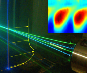
Experiments were conducted in the Large Oscillatory Water and Sediment Tunnel (LOWST) housed in the Ven Te Chow Hydrosystems Laboratory of the University of Illinois at Urbana-Champaign (figure 2). The test section is 12 m long and the internal dimensions of the cross-section are 0.8 m wide by 1.2 m high. A false bed was placed at the middle of the cross-section reducing the height of the water tunnel to 0.6 m. Special attention was given to keeping the smooth PVC bottom fixed rigidly at the middle of the section. External disturbances were kept to a minimum via insulation of the flume from the laboratory floor. The oscillatory motion of the water is driven by three pistons that run inside 0.78 m diameter cylinders with a maximum stroke of 1.37 m. At the opposite end of the tunnel, a 1.0 by 2.0 m holding tank open to the atmosphere acts as a passive receiver for the water displaced by the pistons. Three servo motors, controlled by a computer, drive the pistons using a screw-gear system. Although unidirectional flow was not used in this study, the facility also has two centrifugal pumps that allow for the superposition of a unidirectional current of up to 0.5 m s $^{-1}$ onto the oscillatory motion through a pipe recirculation system. Flow straighteners and sediment traps are available at both ends of the main test section. No sediment particles were used for the present study. LOWST can generate oscillatory flows with time periods between 5 to 15 s and maximum horizontal velocities of up to 2 m s
 $^{-1}$. A more detailed description of the facility can be found in the paper by Pedocchi & García (Reference Pedocchi and García2009b).

Figure 2. Large Oscillatory Water and Sediment Tunnel (LOWST).
Instantaneous velocity measurements were conducted using a three-dimensional laser Doppler velocimetry (LDV) system from TSI Inc., with an Ar-ion 6 W multiline laser (model Stabilite 2017, from Spectra-Physics) generating a light beam which in turn is directed towards a FiberLight $^{\textrm {TM}}$ multicolour beam separator box (model FBL-3). The LDV technique was adopted owing to its high temporal resolution (up to 10 000 Hz), provided that appropriate seeding is achieved in the large oscillatory flow tunnel. This high rate of data sampling (samples per second) ensures that the high frequencies of the flow are preserved, which allows for the analysis of turbulence characteristics, especially within the boundary layer. A preliminary study examined different kinds of seeding particles, which included hollow glass spheres (HGS) and silver-coated hollow glass spheres (S-HGS) of various densities and diameters, as well as different concentrations of particles to ensure a maximum recording rate for the LDV system (Mier Reference Mier2015). The particles used in the experiments were the HGS particles (with a density of 1.1 g cm
 $^{-3}$ and diameter of 11
  $\mathrm {\mu }$m) which are close to neutrally buoyant and are big enough to generate high-intensity backscatter signals, and light enough to meet the turbulence criteria. Preliminary analysis indicated that the optimum concentration (number of particles per unit volume) to ensure a maximum data rate was approximately
  $N=0.1 - 0.2\times V_{m}$, where
  $V_{m}$ is the measurement volume. This analysis took into consideration the effect of light attenuation through the penetration length
  $d_w$ which was equal to 0.4 m (
 $N=0.4 - 0.5\times V_{m}\,\textrm {e}^{\alpha d_{w}}$, where
  $\alpha$ is the attenuation coefficient with values of 7.86 m
 $^{-1}$ for HGS and 5.75 m
 $^{-1}$ for S-HGS). More information can be found in the paper by Mier & García (Reference Mier and García2009). An average value of the diameter of the measurement volume was 0.1 mm and an average value of its length was approximately 1 mm, which resulted in a very small measurement volume (approximately 0.01 mm
 $^3$).
Velocity profiles were measured from a series of vertically distributed pointwise LDV measurements. The LDV probe was mounted on a 3-axis traverse, driven by a microstep controller, capable of providing a spatial resolution of 0.01 mm in all three directions, which was essential for the fine geometric requirements needed inside the boundary layer. The displacement range was approximately 50 cm in all three directions, which allowed for taking measurements across the tunnel. Special attention was given to define the level of the wall where  $y=0$ m (i.e. no-slip boundary condition).
A set of magnets, one mounted on the moving pistons and one on the enclosing cylinders of the flume, was used to synchronize the time instances that define the beginning of each cycle. The present work focuses on the examination of OBL flows with a period of 10 s, which is a typical period for coastal wave applications. In the present work, 130 cycles, in each test, were used for the estimation of turbulence statistics for each phase. Sleath (Reference Sleath1987) argued that 50 periods are enough for the statistics to converge. Jensen et al. (Reference Jensen, Sumer and Fredsøe1989) performed a similar analysis confirming Sleath's findings. A similar analysis of our results shows that negligible variations (typically less than 1 %) were observed for a higher number of cycles.
A summary of the examined cases is presented in table 1. Temperature measurements were conducted to estimate any significant viscosity or density variations. The temperature of the water was kept constant over the time of each experiment. The measured temperatures are also reported in table 1.
Table 1. Test conditions of pure oscillatory flow. Period of the motion  $T=10$ s. Amplitude of the oscillation
  $\alpha =U_{o}T/\nu$. Kinematic viscosity
  $\nu ={1.79\times 10^{-6}}/{(1+0.03368T_{C}+0.00021T_{C}^{2})}$ and density
  $\rho =1000 ( 1- {(T_{C}+288.9414 )(T_{C}-3.9863 )^{2}}/{508929.2(T_{C}+68.1293 )})$.

Ensemble averaging was used to estimate the mean values of all quantities as
 \begin{equation} \bar{u}(y,\omega t)=\frac{1}{N}\sum_{k=0}^{N}u(y,\omega (t+kT))) \end{equation}
The instantaneous fluctuations were calculated as
 \begin{equation} {u}'(y,\omega t)=u(y,\omega (t+kT))-\bar{u}(y,\omega t)) \end{equation}
The root-mean-square (r.m.s.) of the velocity fluctuations and Reynold shear stresses were calculated as
 $$\begin{gather} (\overline{{u}'^2})^{{1}/{2}}(y,\omega t)= \left\{\frac{1}{N}\sum_{k=0}^{N}{u}'^{2}(y,\omega(t+kT))\right\}^{{1}/{2}} \end{gather}$$
 $$\begin{gather}-\overline{{u}'{v}'}(y,\omega t)=\frac{1}{N}\sum_{k=0}^{N}{u}'(y,\omega(t+kT)){v}'(y,\omega(t+kT)) \end{gather}$$
3. Results and discussion
3.1. Mean flow structure and boundary layer properties
3.1.1. Flow regimes
Akhavan et al. (Reference Akhavan, Kamm and Shapiro1991a) and Ramaprian & Tu (Reference Ramaprian and Tu1983) used dimensional analysis and examined the similarity laws of oscillatory and pulsatile pipe flows, respectively. They considered that the OBL flows can be categorized into four regimes based on three length scales: a geometrical length scale based on the diameter of the pipe  $R$, an inertia length scale
  $\delta _{t}= u_{*} / \omega$ and a viscous length scale
  $\delta _{v}= \nu / u_{*}$. It is worth noting that the Stokes length scales with the geometric mean of inertia and viscous length scales (
 $\delta \sim \sqrt {\delta _{t}\delta _{v}}$). Akhavan et al. (Reference Akhavan, Kamm and Shapiro1991a) showed the dimensional necessity for a logarithmic layer to exist when two or more of the scales
  $R$,
$R$,  $\delta _{t}$ and
  $\delta _{v}$ are widely separated.
Based on the above scales, four different cases of oscillatory pipe flows are defined (Akhavan et al. Reference Akhavan, Kamm and Shapiro1991a): (a) Case I, the pipe diameter-limited, ‘quasi-steady’ turbulent behaviour for which  $\delta _{t}\gg R \gg \delta _{v}$ (i.e.
  $u_{*}/(\omega R)\gg 1$,
  $Ru*/\nu \gg 1$), where the flow behaves in a quasi-steady way and a universal logarithmic law is valid; (b) Case II, which can in a way be considered as a special version of Case I for which
  $\delta _{t}\sim R \gg \delta _{v}$ (i.e.
  $u_{*}/(\omega R)\sim 1$,
  $u_{*} R/\nu \gg 1$), for which the flow obeys a modified version of the log-law where the universal slope expressed by von Kármán constant
  $\kappa$ may be constant (
 $\kappa =0.41$). However, the value of constant
  $A$ varies over time (
 $A(\omega t)=f(u_{*}/(R \omega ))$); (c) Case III, for which
  $R\gg \delta _{t} \gg \delta _{v}$ (i.e.
  $u_{*}/(\omega R)$,
  $u_{*}^{2}/(\omega \nu ) \gg 1$) and a logarithmic law is valid for
  $y<\delta _{t}$. However, in the outer layer, where
  $y/\delta _{t} \rightarrow \infty$ (i.e.
  $\delta _t=u_{*}/\omega \rightarrow 0$), the flow behaves in an ‘inviscid way’ similar to the case when
  $u_{*}\rightarrow 0$ (assuming that
  $\omega$ is finite). The mean velocity and turbulent moments profiles depend only on
  $R$ and
  $\omega$ values; (d) Case IV, which again can be considered to be a special version of Case III, for which
  $R \gg \delta _{t} \sim \delta _{v}$ (i.e.
  $u_{*}/(\omega R)$,
  $u_{*}^{2}/(\omega \nu ) \sim 1$) and a logarithmic profile is once again valid with
  $A_{s}$ varying over the cycle. Akhavan et al. (Reference Akhavan, Kamm and Shapiro1991a) presented results of pipe flow of case II. Because coastal/wave flow conditions are of interest, flows in the current study belong to the non-diameter-limited cases III and IV but for a closed channel. Considering half the height of the channel (or the hydraulic radius of the channel) as equivalent to
  $R$,
$R$,  $R \gg u_{*}/\omega$ (or
  $u_{*}/(\omega R) \gg 1$ except from the shear stress reversal when
  $u_{*}$ is zero) for all the flows considered in the present study.
The structure of the OBLs was examined by Jensen et al. (Reference Jensen, Sumer and Fredsøe1989) for a wide range of  $ {\textit {Re}}_{\delta }$ (
 $ {\textit {Re}}_{\delta }$ between 257 and 3464). Jensen et al. (Reference Jensen, Sumer and Fredsøe1989) noticed a distinct difference in the boundary layer structure for
  $Re_{\delta }$ of 762 (expressed in the original work as
  $Re_{w}=2.9\times 10^{5}$). This flow exhibited an intermittent turbulent behaviour for which the logarithmic distribution,
  $u^{+}=(1/\kappa ) \ln y^{+} +5.1$, was valid after
  $\omega t=6{\rm \pi} /9$ (
 $120^{\circ }$). An explanation for this different behaviour, given by the authors, indicated that the flow experiences transitional conditions for most of its period. However, no detailed explanation was given about the effect of
  $ {\textit {Re}}_{\delta }$ on the flow structure and consequently its effect on the bed shear stress especially at the transition from the laminar to transitional and to turbulent flow regime. Hino et al. (Reference Hino, Sawamoto and Takasu1976) studied an OBL for
  $ {\textit {Re}}_{\delta }$ of 876 and
  $R/\delta$ of 12.8; however once again, the effect of
  $Re_{\delta }$ variation was not clearly shown as only results from a single flow case were presented. Recently, Kaptein et al. (Reference Kaptein, Duran-Matute, Roman, Armenio and Clercx2019) used large-eddy simulation to examine the effect of the
  $h/\delta$ ratio (where
  $h$ is the height of their domain representing the water depth on oscillatory flows over a flat plate) on the phase difference between free stream velocity and bed shear stress maxima. Their results showed that for
  $h/\delta \geq 40$, velocity, turbulent characteristic and bed shear stress results converged to those for
  $h/\delta \rightarrow \infty$. In the present study
  $R/\delta$ is of the order of 250, which was consider large enough to represent the coastal boundary layer conditions for which
  $R/\delta \rightarrow \infty$.
3.1.2. Laminar flow
To test the accuracy of our measurements, the lowest  $ {\textit {Re}}_{\delta }$ case was examined (experiment 1 with
  $ {\textit {Re}}_{\delta }=254$) and it was compared with an analytical solution. The velocity profile for the laminar regime can be calculated using the following analytical solution:
 \begin{equation} u(y,\omega t)=U_{o}(\sin(\omega t) - \textrm{e}^{{-}y/\delta}\sin(\omega t - y / \delta)) \end{equation}
by differentiating (3.1) and using the definition of viscous shear stress ( $\tau = \rho \nu \partial u / \partial y$) we can estimate the shear stress variation as
  $\tau (y, \omega t)=\sqrt {2} \rho ({U_{o}^{2}}/{ {\textit {Re}}_{\delta }})\,\textrm {e}^{-y/\delta }\sin (\omega t - y / \delta + {\rm \pi}/4)$ and the wall shear stress
  $\tau _{b}$ can easily be calculated for
  $y=0$ as
 \begin{equation} \frac{\tau_{b}}{\rho}=\sqrt{2} \frac{U_{o}^{2}}{ {\textit{Re}}_{\delta}}\sin(\omega t + {\rm \pi}/4) \end{equation}
 In figures 3(a) and 3(b), the analytical profiles for various time instances are plotted for the acceleration and deceleration phases, respectively, together with the experimental observations. The comparison between the analytical and experimental values agrees well. In addition, to evaluate the symmetry of the imposed oscillation from the pistons of the experimental facility, a comparison between the positive and negative parts of the cycle was conducted. Such comparison of these profiles is shown in figure 3(c), in which the measurement of the negative part of the period is multiplied by  $-$1.0. No significant bias or skewness towards the positive or negative direction was observed in our measurements. Finally, figure 3(d) shows a comparison with the bed shear stress measurements, estimated as
  $\tau _{b} = \rho \nu \partial u/\partial y |_{b}$. Once again, the experimental results agree well with the analytical solution above.

Figure 3. Comparison of measurements against analytical solution for laminar regime (Test 1,  $ {\textit {Re}}_{\delta }=254$): (a) streamwise velocity profiles during acceleration,
  $\circ$ measurements, (—–, black) analytical solution; (b) streamwise velocity profiles during deceleration; (c) comparison between positive and negative parts of the period,
  $\circ$ measurements in the positive part,
  $\times$ measurement in the negative part multiplied by
  $-$1.0, (—–, black) analytical solution; (d) measurements of bed shear stress
  $\tau _{b}$ and free stream velocity
  $U_{\infty}$,
  $\circ$ measurements of bed shear stress, (
 $\bullet$, grey) measurements of free stream velocity, (—–, black) analytical solution for bed shear stress
  $\tau _{b}$, – – –
  $U_{\infty}(t)=U_{o}sin(\omega t)$.
3.1.3. Transitional flow
In their work, Hino et al. (Reference Hino, Kashiwayanagi, Nakayama and Hara1983) examined the flow structure for a flow with  $ {\textit {Re}}_{\delta }= 876$. They presented data for the mean flow and turbulence characteristics for this Reynolds number but owing to the fact that only a single flow was analysed, the change of the mean flow characteristics as
  $ {\textit {Re}}_{\delta }$ increased and the flow went through a transition remains unknown. In figure 4, the ensemble average velocity profiles for three characteristic instances of the period (
 ${\rm \pi} /4$,
  ${\rm \pi} /2$ and
  $3{\rm \pi} /4$) are shown for all the examined flows. In figure 4(a–c), the velocity profiles are presented in wall units (where
  $y^{+}=u_{*}y/\nu$,
  $u^{+}=\bar {u}/u_{*}$ and
  $u_{*}$ is the shear velocity
  $u_{*}=\sqrt (\overline {\tau _{b}}/\rho )$). The orange dashed lines show the fit of a logarithmic profile similar to the ‘universal log-law’ for turbulent equilibrium boundary layers. Figures 4(d–f) and 4(g–i) show the velocity defect normalized using the free stream velocity
  $U_{\infty}$ and shear velocity, respectively. The arrows show the general trends of the velocity profiles. Jensen et al. (Reference Jensen, Sumer and Fredsøe1989) have shown that for high enough
  $ {\textit {Re}}_{\delta }$ values the velocity profiles should approach the universal logarithmic-law for a smooth wall:
 \begin{equation} U^{+}=\frac{1}{\kappa}\ln \left(y^{+}\right)+ A_{s} \end{equation}
with  $\kappa \approx 0.41$ and
  $A_{s}\approx 5.1$. For equilibrium boundary layers, (3.3) is valid only for the part of the velocity close to the wall, while far from the wall additional adjusting parameters need to be used to describe the velocity profile, e.g. law of the wake (Krug, Philip & Marusic Reference Krug, Philip and Marusic2017; Jimenez Reference Jimenez2018). Akhavan et al. (Reference Akhavan, Kamm and Shapiro1991a) showed that for
  $ {\textit {Re}}_{\delta }$ in the transitional regime (when
  $u_{*}/\omega \nu \sim 1.$) (3.3) is modified to
  $U^{+}=({1}/{\kappa })\ln (y^{+})+ A_{s}(\omega t)$,
  $A_{s}$ changes for different phases of the period. Hino et al. (Reference Hino, Kashiwayanagi, Nakayama and Hara1983) also showed that
  $A_{s}$ varies for a transitional flow (
 $ {\textit {Re}}_{\delta }=873$). In figures 4(b), 4( f) and 4(i), and to an extent in figures 4(a) and 4(h), it can be observed that the mean profile in the transitional flows and especially for
  $ {\textit {Re}}_{\delta } = 763$ (experiment 5) deviate significantly from both the logarithmic profiles, which are observed for higher
  $ {\textit {Re}}_{\delta }$ cases, and the laminar profiles. However, as
  $ {\textit {Re}}_{\delta }$ increases there is a clear trend towards the equilibrium logarithmic law (
 $A_{s} \approx 5.1$ in (3.3)). The arrows in figure 4(c–i) show this transition.

Figure 4. Reynolds number effect. Ensemble average velocity profiles in wall units for: (a)  $\omega t={\rm \pi} /4$; (b)
  $\omega t={\rm \pi} /2$; (c)
  $\omega t=3{\rm \pi} /4$. Ensemble average velocity defect profile normalized with free stream velocity
  $U_{\infty }$ and
  $\delta$ for: (d)
  $\omega t={\rm \pi} /4$; (e)
  $\omega t={\rm \pi} /2$; ( f)
  $\omega t=3{\rm \pi} /4$. Ensemble average velocity defect profile normalized with shear velocity
  $u_{*}$ for:(h)
  $\omega t={\rm \pi} /4$; (i)
  $\omega t={\rm \pi} /2$; (g)
  $\omega t=3{\rm \pi} /4$. Dashed orange lines show logarithmic fit for the cases with
  $ {\textit {Re}}_{\delta } \geq 763$. The arrows show the increasing
  $ {\textit {Re}}_{\delta }$ path.
To evaluate the fit of the logarithmic profiles, the log-law diagnostic function  $\varXi$ (
 $\varXi =y^{+}({\partial \bar {{u}}^{+}}/{\partial y^{y}})$) is plotted in figure 5 for three
  $ {\textit {Re}}_{\delta }$ (763, 937 and 1315) for
  $\omega t={\rm \pi} /2$ to
  $5{\rm \pi} /6$. The
  $\varXi$ function should approach
  $1/\kappa$ for zero-pressure gradient boundary layers in regions where the log-law occurs (Nagib, Chauhan & Monkewitz Reference Nagib, Chauhan and Monkewitz2007). In addition to the equilibrium value
  $1/\kappa$, the
  $1/\kappa (\omega t)$ values are also plotted for each profile. It can be seen that for
  $ {\textit {Re}}_{\delta }=763$ (experiment 5) the part of the profile where a logarithmic equation may fit is smaller compared with the higher
  $ {\textit {Re}}_{\delta }$ cases. For this flow, the slope of the logarithmic profile will be larger than 1/0.41. As
  $ {\textit {Re}}_{\delta }$ increases to 937 and 1315 we can observe that the log profile slope
  $1/\kappa (\omega t)$ starts to approach 1/0.41 for parts of the deceleration. Furthermore, the region where a logarithmic profile may fit increases in size. Finally, for
  $ {\textit {Re}}_{\delta }=1315$ the profiles seem to agree well with the
  $1/0.41$ slope, although the slope becomes smaller towards
  $\omega t = 5{\rm \pi} /6$. It is important to note that in our work the use of
  $\kappa$ (velocity profile's slope) and
  $A_{s}$ (velocity profile's intersect) for the parts of the flow that are not in equilibrium (e.g. the values for
  $\omega t<{\rm \pi} /2$) is merely to provide us with a diagnostic parameter for the development of a true logarithmic profile. This same approach has been used in the past specifically for the case of OBL flows by Hino et al. (Reference Hino, Kashiwayanagi, Nakayama and Hara1983) (figures 7 and 9 in their original work) and by Akhavan et al. (Reference Akhavan, Kamm and Shapiro1991a) (figures 19 and 23 in their original work). The values of
  $\kappa$ and
  $A_{s}$ are obtained by fitting the logarithmic law in a region of approximately
  $30\le y^{+} \le 150$. The region where a logarithmic layer exists varies over time and for different
  $ {\textit {Re}}_{\delta }$ values. However, the region of the fit was chosen with the aims to maximize the region of the fitting but also to avoid the wake effects (Krug et al. Reference Krug, Philip and Marusic2017).

Figure 5. Log-law diagnostic function  $\varXi$ during the deceleration phase for
  $ {\textit {Re}}_{\delta }$ values of
  $763$,
  $937$ and
  $1315$.
Akhavan et al. (Reference Akhavan, Kamm and Shapiro1991a) argued that  $A_{s}$ should approach an equilibrium value for oscillatory pipe flows when
  $u_{*}^2/\omega \nu \gg 1$ (and
  $u_{*}/\omega R \ll 1$). Their analysis did not include cases for
  $u_{*}^2/\omega \nu \gg 1$. Instead they referred to the works of Mizushina, Maruyama & Shiozaki (Reference Mizushina, MARUYAMA and Shiozaki1974) and Ramaprian & Tu (Reference Ramaprian and Tu1983) who examined conditions of
  $u_{*}^2/\omega R \approx 0.1$ and
  $u_{*}^2/\omega \nu \approx 100$. The present analysis extends significantly the ranges of Akhavan et al. (Reference Akhavan, Kamm and Shapiro1991a), Mizushina et al. (Reference Mizushina, MARUYAMA and Shiozaki1974) and Ramaprian & Tu (Reference Ramaprian and Tu1983).
3.2. Boundary layer thickness
Different characteristic length scales have been proposed in the literature to characterize the thickness of oscillatory boundary layers. Sumer, Jensen & Fredsøe (Reference Sumer, Jensen and Fredsøe1987) defined the thickness of the boundary layer  $\delta _{{\rm \pi} /2}$ based on the velocity maximum at
  $\omega t = {{\rm \pi} }/{2}$. Similar definitions have been used by Sleath (Reference Sleath1987) and Jonsson & Carlsen (Reference Jonsson and Carlsen1976) for
  $\omega t = {{\rm \pi} }/{2}$ but instead of the maximum velocity they used the 5 % defect of the velocity with respect to the free stream value and the first
  $y$-position from the wall where
  $\bar {{u}}$ equals the free stream velocity, respectively. Jensen et al. (Reference Jensen, Sumer and Fredsøe1989) plotted their results of
  $\delta _{{\rm \pi} /2}$ for two flow conditions (
 $ {\textit {Re}}_{\delta }$ of
  $1789$ and
  $3464$). They also compared their results with those of Hino et al. (Reference Hino, Kashiwayanagi, Nakayama and Hara1983) and Spalart & Baldwin (Reference Spalart, Baldwin and André1989). In figure 6 the boundary thickness is plotted based on the definition of Sumer et al. (Reference Sumer, Jensen and Fredsøe1987). The values are normalized using the amplitude of the oscillation
  $\alpha$. The definition of
  $\delta _{{\rm \pi} /2}/\alpha$ is also shown in the inset of the plot. The prediction of the analytical solution
  ${\delta _{{\rm \pi} /2}}/{\alpha }=({3{\rm \pi} }/{4})({4}/{ {\textit {Re}}_{\delta }^{2}})^{{1}/{2}}$ and the solution by Fredsøe (Reference Fredsøe1984) are also plotted together with the previous data of Jensen et al. (Reference Jensen, Sumer and Fredsøe1989), Hino et al. (Reference Hino, Kashiwayanagi, Nakayama and Hara1983) and Spalart & Baldwin (Reference Spalart, Baldwin and André1989). The experimental observations of the present work match reasonably well with the laminar solution for
  $ {\textit {Re}}_{\delta }$ of
  $254$ and
  $405$ (experiments 1 and 2). The rest of the data (experiments 3–10) connect the laminar with the turbulent regimes. Specifically, as the
  $ {\textit {Re}}_{\delta }$ increases,
  $\delta _{{\rm \pi} /2}/\alpha$ seems to increase until
  $ {\textit {Re}}_{\delta } \approx 1500$ when the turbulent solution of Fredsøe (Reference Fredsøe1984) predicts well the behaviour of the experiments by Jensen et al. (Reference Jensen, Sumer and Fredsøe1989). The results of the present study agree well with the results of Hino et al. (Reference Hino, Kashiwayanagi, Nakayama and Hara1983) and Spalart & Baldwin (Reference Spalart, Baldwin and André1989), which are in a similar range of
  $ {\textit {Re}}_{\delta }$ values.

Figure 6. Normalized oscillatory boundary layer thickness  $\delta _{{\rm \pi} /2}/\alpha$ as a function of
  $ {\textit {Re}}_{\delta }$ or
  $ {\textit {Re}}_{w}$.
For their analysis, Jensen et al. (Reference Jensen, Sumer and Fredsøe1989) used the maximum velocity of each ensemble-averaged profile to define the boundary layer thickness  $y_{max}$ for each phase (for this location also shear stress is
  $\bar {{\tau }} \approx 0$). For this analysis, the same approach used by Jensen et al. (Reference Jensen, Sumer and Fredsøe1989) was adopted. No significant changes in the results of the analysis were observed when
  $\bar {{\tau }} \approx 0$ was used instead of
  $\bar {{u}}|_{max}$ for the definition of the boundary layer. A plot of boundary layer thickness for all the examined cases together with the ensemble-averaged contours of streamwise velocity are shown in figure 7. The results are made dimensionless using the Stokes length
  $\delta$. In addition to the boundary layer thickness, the displacement thickness
  $\delta _{*}$ and momentum thickness
  $\theta$ are plotted in figure 7, which are defined as
 $$\begin{gather} \delta_{*}(\omega t)=\int_{0}^{y_{max}}\frac{U_{\infty}(\omega t)-\bar{u}(y,\omega t)}{U_{\infty} (\omega t)}\,{\textrm{d}y}, \end{gather}$$
 $$\begin{gather}\theta(\omega t)=\int_{0}^{y_{max}} \frac{\bar{u}(y,\omega t)}{U_{\infty}(\omega t)} \left(\frac{U_{\infty}(\omega t)-\bar{u}(y,\omega t)}{U_{\infty}(\omega t)} \right) {\textrm{d}y}, \end{gather}$$
where  $U_{\infty }(\omega t)$ is the free stream velocity over time and
  $y_{max}(\omega t)$ is the boundary layer thickness. Based on the displacement and momentum thickness, the shape factor
  $H$ is defined as
  $H=\delta _{*}/\theta$. A value between
  $H=1.3 - 1.5$ is typical for turbulent unidirectional flows. The prediction of displacement thickness and momentum thickness normalized with the Stokes length are shown in figure 7 together with the corresponding
  $H$ factors. For reference,
  $H=1.4$ is plotted as a threshold value for equilibrium boundary layers.
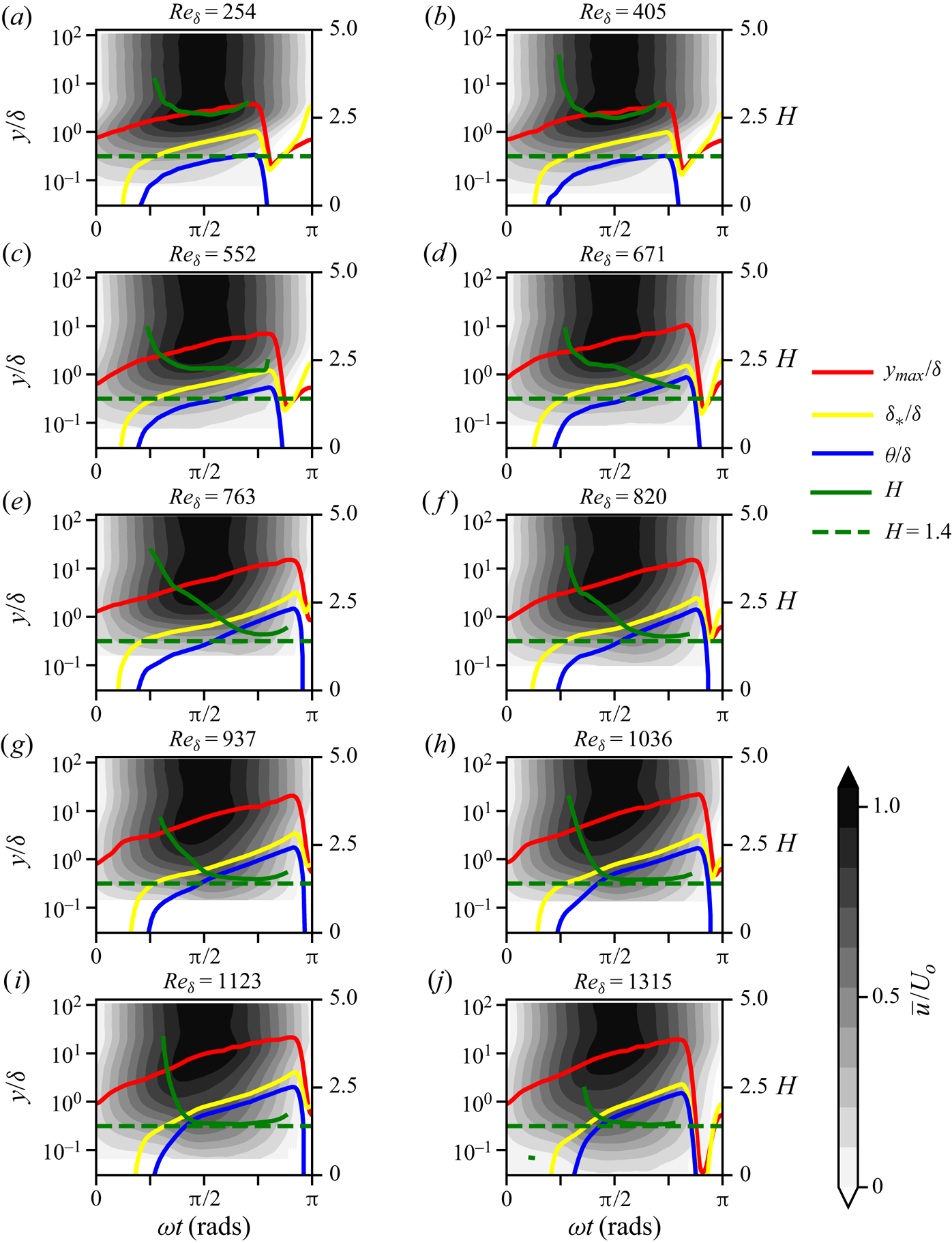
Figure 7. Contour maps of normalized velocity profiles  $\bar {{u}}/U_{o}$. Dimensionless boundary layer thickness
  $y_{max}/\delta$, displacement thickness
  $\delta _{*}/\delta$, momentum thickness
  $\theta /\delta$ and shape factor
  $H$. The typical value of
  $H=1.4$ for fully developed unidirectional flow is also shown.
It can be observed that the boundary layer thickness continues to grow even during the deceleration phase. As  $ {\textit {Re}}_{\delta }$ increases, the normalized boundary thickness
  $y_{max}/\delta$ also increases. It is worth noting that owing to the characteristic near-bed overshoot with respect to the free stream velocities (see e.g. figures 3(a) or 4), both the displacement thickness and momentum thickness have negative values at the beginning of the acceleration phase. Displacement and momentum thickness maxima increase with
  $ {\textit {Re}}_{\delta }$. Initially, for the low
  $ {\textit {Re}}_{\delta }$ cases,
  $H$ stays high (
 $\sim 2.5$). As
  $ {\textit {Re}}_{\delta }$ increases (especially for
  $ {\textit {Re}}_{\delta } \geq 763$), the shape factor approaches a value of 1.4 at the middle of the deceleration phase. This part of the period is associated with enhanced turbulent fluctuations (Hino et al. Reference Hino, Kashiwayanagi, Nakayama and Hara1983; Fishler & Brodkey Reference Fishler and Brodkey1991; Carstensen et al. Reference Carstensen, Sumer and Fredsøe2010, also see § 3.4). The shape factor increases again near the bed shear stress reversal. For higher
  $ {\textit {Re}}_{\delta }$ values, the shape factor approaches the value of 1.4 earlier, towards the end of the acceleration phase.
Figure 7 shows the boundary layer thickness increase during the deceleration phase. It is important to note here that the boundary layer thickness was considered to be zero when near-bed reversal occurred. The difficulties associated with the measurements of bed shear stress and velocity profiles at a boundary layer which is on the verge of separation may explain the discrepancies at the instance when the boundary layer thickness drops in figure 7. These discrepancies can also be observed in previous works in the literature, e.g. significant scatter has been reported by Carstensen et al. (Reference Carstensen, Sumer and Fredsøe2010) at the instance when near-bed flow reversal occurs (figure 10 in their paper).
3.3. Friction coefficient and phase difference
3.3.1. Bed shear stress and friction coefficient
Jensen et al. (Reference Jensen, Sumer and Fredsøe1989) presented time series of the bed shear stress variation over an oscillation period for a wide range of flows. Also included were the experimental observations by Hino et al. (Reference Hino, Kashiwayanagi, Nakayama and Hara1983) and the direct numerical simulation results of Spalart & Baldwin (Reference Spalart, Baldwin and André1989). The purpose of the present work is to examine in more detail the behaviour of bed shear stress in the transitional regime (and especially for  $550 \le {\textit {Re}}_{\delta } \le 1000$), for which only limited data are available in the literature, i.e. by Hino et al. (Reference Hino, Kashiwayanagi, Nakayama and Hara1983) (
 $ {\textit {Re}}_{\delta }=876$), Spalart & Baldwin (Reference Spalart, Baldwin and André1989) (
 $ {\textit {Re}}_{\delta }=800$ and
  $1000$) and Jensen et al. (Reference Jensen, Sumer and Fredsøe1989) (
 $ {\textit {Re}}_{\delta }=762$). In this regime some inconsistencies have also been noticed in the literature regarding the phase when the maximum bed shear stress occurs with respect to the maximum free stream velocity (
 ${\rm \Delta} \phi$ in figure 3) (see § 3.3.2). In the present study the bed shear stress is estimated using the following:
 \begin{equation} \frac{\overline{\tau}_{b}}{\rho}=\nu\frac{\partial \bar{u}}{\partial y} - \overline{{u}'{v}'} \end{equation}
The gradient of the ensemble-average velocity is typically estimated over the 3–4 nearest points (which typically are within a distance of less than 0.2 mm from the wall) to ensure accurate estimation of the gradient. Also, for all the examined flows the second term of (3.6) is nearly zero; this arises from the fact that the first points of measurement are usually inside the viscous sublayer. This is typically the case for both unidirectional (e.g. Nezu & Nakagawa Reference Nezu and Nakagawa1993) as well as oscillatory flows (e.g. see the DNS results of Spalart & Baldwin (Reference Spalart, Baldwin and André1989) or the experimental observations by Hino et al. Reference Hino, Kashiwayanagi, Nakayama and Hara1983).
Another way to estimate the bed shear stress is by using the integral of the momentum equation (Hino et al. Reference Hino, Kashiwayanagi, Nakayama and Hara1983; Jensen et al. Reference Jensen, Sumer and Fredsøe1989):
 \begin{equation} \left(\frac{\bar{{\tau}}_{b}}{\rho} \right)=\left(\frac{\bar{{\tau}}}{\rho} \right)_{wall}= \int_{0}^{D}\frac{\partial}{\partial t}\left(U_{\infty}(\omega t)-\bar{u}(y,\omega t)\right){\textrm{d}y} \end{equation}
Hino et al. (Reference Hino, Kashiwayanagi, Nakayama and Hara1983) used half the height of the cross-section as distance  $D$, while Jensen et al. (Reference Jensen, Sumer and Fredsøe1989) used the boundary layer thickness
  $y_{max}$ (see appendix B in the paper by Jensen Reference Jensen1989). In the present work, the approach of Jensen (Reference Jensen1989) was adopted.
Throughout the present work,  $\tau _{b}$ results were obtained using (3.6), because that method is better suited than (3.7) considering the type of measurements performed (point-wise LDV measurements close to the wall, even inside the viscous sublayer). Some discrepancies between the computed values using (3.6) and (3.7) are consistent with the observations by Hino et al. (Reference Hino, Kashiwayanagi, Nakayama and Hara1983) and Jensen (Reference Jensen1989) for OBL flows and by Coles (Reference Coles1956) for unidirectional boundary layers. The latter argued that the momentum integral equation may introduce large errors for flow under a pressure gradient, especially close to flow reversal. Although the main results of the present analysis do not seem to be sensitive to the choice between (3.6) and (3.7), (3.6) has been adopted for the rest of the analysis.
For comparison, the normalized bed shear stress ( $\overline {\tau _{b}}/\overline {\tau }_{b_{max}}$) computed using (3.6) and (3.7) are shown in figure 8, where
  $\overline {\tau }_{b_{max}}$ is the maximum of the ensemble-average bed shear stress. In addition, the corresponding results by Hino et al. (Reference Hino, Kashiwayanagi, Nakayama and Hara1983) and Jensen et al. (Reference Jensen, Sumer and Fredsøe1989) are plotted. These studies had examined flows with slightly different
  $ {\textit {Re}}_{\delta }$ compared with those in the present analysis. These
  $ {\textit {Re}}_{\delta }$ values are shown in figure 8 in grey. From the results, it becomes obvious that two peaks, one associated with the laminar regime (
 $\circ$) and one associated with the intermittent-turbulent/turbulent regime (
 $\bullet$), exist. Depending on the
  $ {\textit {Re}}_{\delta }$, one of the two peaks becomes larger. The absolute maximum is also shown in figure 8 by (
 ${\bigcirc}$, grey). For low
  $ {\textit {Re}}_{\delta }$ values (
 $ {\textit {Re}}_{\delta } < 552$) only a single peak exists. The second peak which is related also to the transition to turbulence starts to occur for
  $ {\textit {Re}}_{\delta }=552$. This is consistent with the experimental observations by Fishler & Brodkey (Reference Fishler and Brodkey1991) and Hino et al. (Reference Hino, Sawamoto and Takasu1976) who measured significant turbulent bursts during the deceleration phase in flows of similar
  $ {\textit {Re}}_{\delta }$. For
  $ {\textit {Re}}_{\delta }$ of
  $671$ the second ‘turbulent’ peak increases but still remains small compared with the ‘laminar’ peak. It is at
  $ {\textit {Re}}_{\delta }=763$ when the ‘turbulent’ peak becomes larger than the ‘laminar’ peak. This behaviour of a gradually increasing second peak continues until
  $ {\textit {Re}}_{\delta }=1036$. For
  $ {\textit {Re}}_{\delta } > 1036$ the ‘laminar’ peak is absorbed by the strength of the ‘turbulent’ peak.

Figure 8. Normalized bed shear stress  $|\overline {\tau }_{b}|/\overline {\tau }_{b_{max}}$ for various
  $ {\textit {Re}}_{\delta }$. The peaks associated with the laminar regime are shown with
  $\circ$ and the peaks associated with the ‘turbulent’/‘transitional’ regime are shown with
  $\bullet$. The maximum of the two peaks is shown with (
 ${\bigcirc}$, grey). The
  $ {\textit {Re}}_{\delta }$ values for the data by Hino et al. (Reference Hino, Kashiwayanagi, Nakayama and Hara1983) and Jensen (Reference Jensen1989) are shown in grey text.
It is important also to comment on the time instance when the maximum shear stress occurs. The ‘turbulent’ peaks start to occur towards the middle of the deceleration phase. As the values of these peaks increase, the absolute maximum of the bed shear stress starts occurring earlier during the deceleration phase. In other words, the bed shear stress maximum ‘lags’ with respect to the free stream velocity maximum (which takes place always at  $\omega t = {\rm \pi}/2$). Although this behaviour has been observed in the literature, no detailed analysis has ever been performed to examine the presence of this phase lag and how the phase difference changes in the transitional regime. This was the main motivation for the present study. The authors suggest that the ‘phase lead’ diagram of Jensen et al. (Reference Jensen, Sumer and Fredsøe1989), which is included in many classic textbooks on coastal engineering and coastal boundary layers (e.g. Fredsøe & Deigaard Reference Fredsøe and Deigaard1992), needs to be revised to take into consideration the presence of the phase lag. More about this point will be discussed in § 3.3.2.
The behaviour of the bed shear stress time series, presented in figure 8, is consistent with the published values of Reynolds number separating the different OBL flow regimes. In the introduction, the disturbed laminar regime was defined as a regime in which the flow behaves like in the laminar regime, but small perturbations are superimposed on the OBL flow. This kind of linear instability-related disturbances (Carstensen et al. Reference Carstensen, Sumer and Fredsøe2010) are not sufficiently strong to alter the mean velocity profiles. Figure 3 showed the excellent agreement between our measurements for  $ {\textit {Re}}_{\delta }=254$ and the laminar solution. These linear instability-related features are extremely difficult to be captured using the applied pointwise measurement technique (i.e. LDV). However, it is worth noting that the second ‘turbulent peak’ of the bed shear stress starts to appear for
  $ {\textit {Re}}_{\delta }=552$, which is very close to the threshold value for the intermittently turbulent regime (Pedocchi et al. Reference Pedocchi, Cantero and García2011; Ozdemir et al. Reference Ozdemir, Hsu and Balachandar2014).
In addition to bed shear stress variation over a period, also of interest is the maximum bed shear stress and its variation as a function of  $ {\textit {Re}}_{\delta }$. Numerous studies in the literature deal with the estimation of the maximum bed shear stress over the period, usually expressed in terms of the friction factor
  $f_{w}$ (e.g. Jonsson Reference Jonsson1966; Kamphuis Reference Kamphuis1975; Sarpkaya Reference Sarpkaya1993), where
  $f_{w}=2({\overline {\tau }_{b_{max}}}/{\rho })/U_{o}^{2}$. Effects of roughness height, which is usually expressed using the relative ratio
  $\alpha /k_{s}$ (e.g. Jonsson Reference Jonsson1966; Kamphuis Reference Kamphuis1975), and flow regime using a form of
  $Re_{*}=u_{*}k_{s}/\nu$ (e.g. Pedocchi & García Reference Pedocchi and García2009a) have also been examined (note that here
  $k_{s}$ is an effective Nikuradse roughness, usually estimated using a characteristic bed particle diameter, García Reference García2008).
In figure 9 the friction factor  $f_{w}$ as a function of
  $ {\textit {Re}}_{\delta }$ is plotted together with data from previous studies in the literature. A second abscissa axis is added showing the values of
  $ {\textit {Re}}_{w}$ arising from the fact that some works have defined the Reynolds number using half of the oscillation amplitude (
 $ {\textit {Re}}_{w}= {\textit {Re}}_{\delta }^{2}/2$). The prediction of the laminar solution and the semi-empirical theoretical solution of Fredsøe (Reference Fredsøe1984) are also shown. In general, a good agreement is observed between the data from this study and the experimental and theoretical results in the literature. Data of Kamphuis (Reference Kamphuis1975) seem to underestimate the friction coefficient (by a factor of
  $\sim 20\,\%$) compared with the rest of the datasets. The observed
  $f_{w}$ results are reasonably close to the measurements of Hino et al. (Reference Hino, Kashiwayanagi, Nakayama and Hara1983), Jensen et al. (Reference Jensen, Sumer and Fredsøe1989), Sarpkaya (Reference Sarpkaya1993) and Carstensen et al. (Reference Carstensen, Sumer and Fredsøe2010), and the DNS results of Spalart & Baldwin (Reference Spalart, Baldwin and André1989). For higher
  $ {\textit {Re}}_{\delta }$ values (
 $ {\textit {Re}}_{\delta } > 1123$) the results are close to the experimental observations of Jensen et al. (Reference Jensen, Sumer and Fredsøe1989) and Carstensen et al. (Reference Carstensen, Sumer and Fredsøe2010) but start to deviate from the observations by Sarpkaya (Reference Sarpkaya1993).
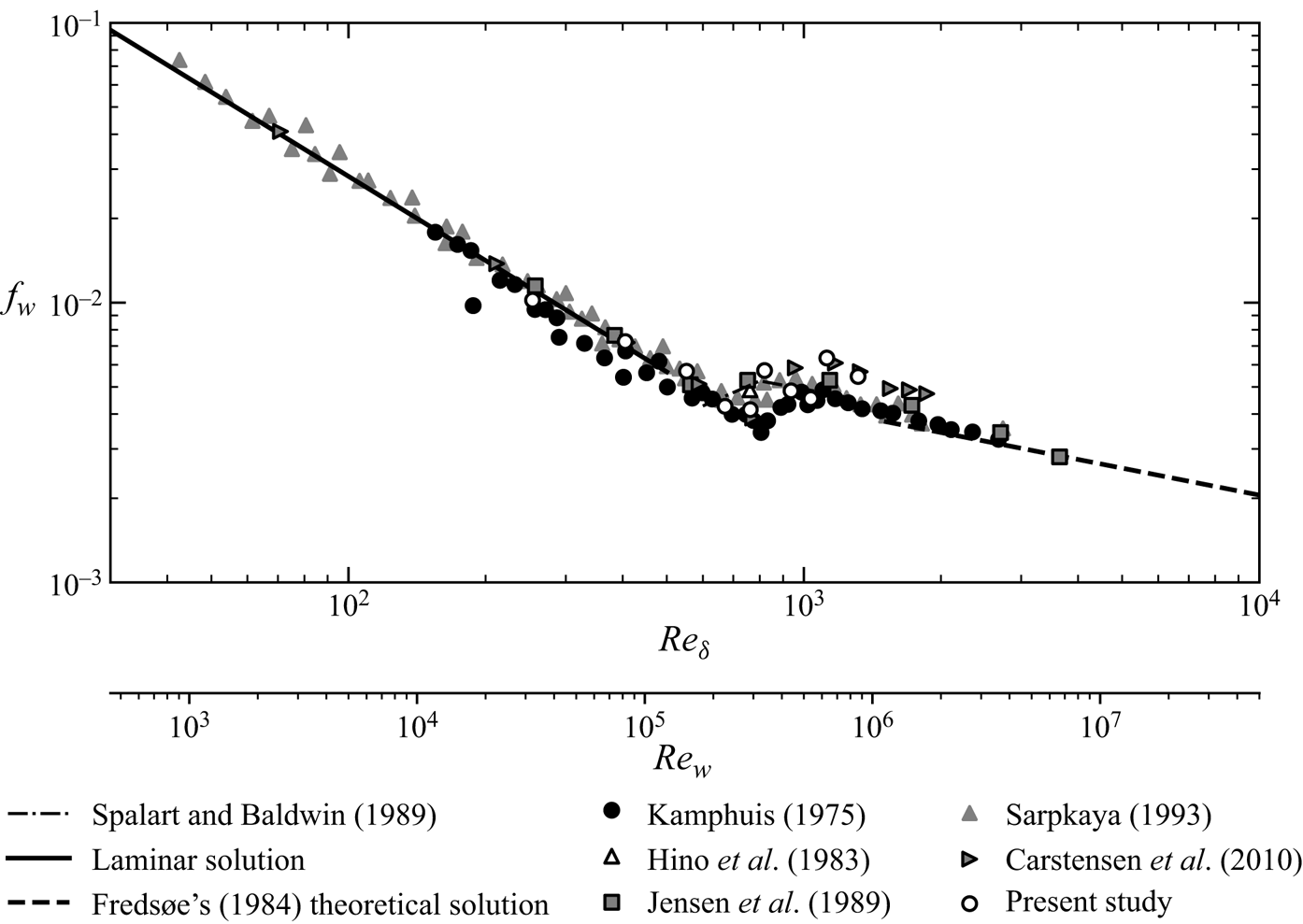
Figure 9. Friction factor  $f_{w}$ as a function of
  $ {\textit {Re}}_{\delta }$ and
  $ {\textit {Re}}_{w}$.
3.3.2. Phase difference
Hino et al. (Reference Hino, Sawamoto and Takasu1976) measured the near bed velocity time series and showed that the velocities experience significant fluctuations during the deceleration phase. These spikes increase in magnitude as  $ {\textit {Re}}_{\delta }$ increases. The moment during the period when these spikes in the velocity signal start to appear also varies with
  $ {\textit {Re}}_{\delta }$, starting earlier for higher
  $ {\textit {Re}}_{\delta }$ and moving towards the end of the acceleration phase (see Hino et al. Reference Hino, Sawamoto and Takasu1976, pp. 200–201, figures 6, 7 and 8). These velocity fluctuations are associated with a peak in the phase-averaged bed shear stress that follows a similar peak in r.m.s. fluctuations. In fact, this behaviour was also shown in the ensemble-average wall shear stress measurements by Hino et al. (Reference Hino, Kashiwayanagi, Nakayama and Hara1983, p. 373, figure 10). Jensen et al. (Reference Jensen, Sumer and Fredsøe1989) measured the bed shear stress variation over the circle of an oscillation. From their analysis, the fluctuation of bed shear stress can be used to determine the inception of turbulence. Starting from the laminar regime and as
  $ {\textit {Re}}_{\delta }$ increases, bed shear stress fluctuations start appearing at the deceleration point near bed shear stress reversal. In the transitional regime, these fluctuations increase in magnitude and appear earlier during the period as flow Reynolds number increases. From figure 9 in the paper by Jensen et al. (Reference Jensen, Sumer and Fredsøe1989) it is clear that actually the maximum bed shear stress occurs after the maximum velocity instance for the case of
  $ {\textit {Re}}_{\delta }=726$ (this value corresponds to
  $ {\textit {Re}}_{w}$ of
  $2.9\times 10^5$ based on the different Reynolds number
  $ {\textit {Re}}_{w}$ adopted by Jensen et al. Reference Jensen, Sumer and Fredsøe1989). However, it is worth pointing out that both Hino et al. (Reference Hino, Kashiwayanagi, Nakayama and Hara1983) and Jensen et al. (Reference Jensen, Sumer and Fredsøe1989) did not comment on the presence of a phase lag in their results. Instead, they reported only the laminar peak of the bed shear stress, as it is shown in figure 1. Carstensen et al. (Reference Carstensen, Sumer and Fredsøe2010) studied coherent structures development in oscillatory flows with gradually increasing oscillation amplitude but constant period. In their study, they conducted a comprehensive analysis of coherent structures by means of flow visualization while the effect of these structures on bed shear stress was examined quantitatively using bed shear stress measurements with a hot-film probe. Despite the fact that their measurements were mainly instantaneous, similar conclusions regarding the phase difference
  ${\rm \Delta} \phi$ can be drawn after careful inspection of their bed shear stress measurements. In figures 15 and 16 of their work, the instantaneous bed shear stress measurements are plotted. The range of the flows is for
  $ {\textit {Re}}_{\delta }$ values between 616 and 1288 for figure 15 (these values correspond to
  $ {\textit {Re}}_{w}$ between
  $1.9\times 10^5$ and
  $8.3 \times 10^5$, based on the different Reynolds number adopted by Carstensen et al. Reference Carstensen, Sumer and Fredsøe2010), and between 1549 and 3162 for figure 16. Close examination of these instantaneous data shows that the actual maximum bed shear stress is delayed by approximately 45
 $^{\circ}$ for
  $ {\textit {Re}}_{\delta }=616$. This phase lag between maximum bed shear stress and maximum velocity decreases as
  $ {\textit {Re}}_{\delta }$ increases (equalling 734, 812, 892 and 969). As the Reynolds number further increases, it becomes difficult to exactly evaluate the time instance when the maximum bed shear stress is reached; however, it can still be seen that the phase of the maximum bed shear stress shifts closer to the maximum velocity instance. The above observations also motivated the present experimental analysis.
Previous numerical studies have also shown the presence of a phase lag at the intermittent turbulent regime (Spalart & Baldwin Reference Spalart, Baldwin and André1989; Vittori & Verzicco Reference Vittori and Verzicco1998; Costamagna et al. Reference Costamagna, Vittori and Blondeaux2003; Bettencourt & Dias Reference Bettencourt and Dias2018). Figure 2 in the paper by Spalart & Baldwin (Reference Spalart, Baldwin and André1989) shows that for  $ {\textit {Re}}_{\delta }=600$ there is a ‘phase lead’ of the bed shear stress with respect to free stream velocity while bed shear stress lags with respect to the free stream velocity for
  $ {\textit {Re}}_{\delta }=800$. This means that there is a threshold value for
  $ {\textit {Re}}_{\delta }$ for which the phase difference between bed shear stress and free stream velocity maximum shifts to negative values. In figure 3 from the paper by Spalart & Baldwin (Reference Spalart, Baldwin and André1989) it is also shown that the phase lag decreased for a higher
  $ {\textit {Re}}_{\delta }=1000$. Similar values of phase difference have been obtained using DNS by Vittori & Verzicco (Reference Vittori and Verzicco1998) (figure 19 in their paper for
  $ {\textit {Re}}_{\delta }=1000$), Costamagna et al. (Reference Costamagna, Vittori and Blondeaux2003) (figure 5 in their paper for
  $ {\textit {Re}}_{\delta }$ 740 and 1120), and one-dimensional modelling of oscillatory boundary layer flows by Hanjalić, Jakirlić & Hadžić (Reference Hanjalić, Jakirlić, Hadžić and Durst1995) and Cotton et al. (Reference Cotton, Craft, Guy and Launder2001).
The observations in the present study for the phase difference  ${\rm \Delta} \phi$ between free stream and bed shear stress maxima are plotted together with other data in the literature in figure 10. It is worth noting that all the data from the literature that showed phase lag are plotted with the appropriate negative
  ${\rm \Delta} \phi$ values. The prediction of the analytical (
 ${\rm \Delta} \phi = {{\rm \pi} }/{4}$) and the theoretical solution of Fredsøe (Reference Fredsøe1984) are also shown. The results found in the literature seem to agree reasonably well with the observations in this study. For flows in the laminar regime, bed shear stress maxima seem to lead the free stream velocity maxima by the standard
  ${\rm \pi} /4$ rads. As the
  $ {\textit {Re}}_{\delta }$ increases further and the flows approach the end of the ‘disturbed-laminar’ and the beginning of the ‘intermittent turbulent’ regime, this phase lead decreases (note that after
  $ {\textit {Re}}_{\delta }=550$ the second/‘turbulent’ peak of the bed shear stress is increasing). At a threshold value of
  $ {\textit {Re}}_{\delta }=763$ a phase lag, i.e. negative
  ${\rm \Delta} \phi$, is observed as the second ‘transition to turbulence’-related peak becomes larger. This peak happens earlier and earlier as the
  $ {\textit {Re}}_{\delta }$ value increases, until it turns to positive values again for
  $ {\textit {Re}}_{\delta }\sim 1000$. For
  $ {\textit {Re}}_{\delta } > 1450$ the phase difference seems to be predicted well using the theoretical solution of Fredsøe (Reference Fredsøe1984). In the authors opinion, this modified diagram is the main contribution from the work presented herein and it has important implications in the fields of coastal engineering, sediment transport and morphodynamics. Of relevance to the analysis of the phase lag is the second burst of sediment entrainment, which is commonly observed in oscillatory sheet flows (Ribberink et al. Reference Ribberink, Dohmen-Janssen, Hanes, McLean and Vincent2000, Reference Ribberink, van der Werf, O'Donoghue and Hassan2008; Nielsen, van der Wal & Gillan Reference Nielsen, van der Wal and Gillan2002). Similar sediment entrainment bursts during the deceleration phase have been observed in time-varying flows by Admiraal, García & Rodriguez (Reference Admiraal, García and Rodriguez2000). In the following section, turbulence parameters will be presented in an effort to elucidate the changes of the flow structure that are associated with the phase difference between bed shear stress and free stream velocity.

Figure 10. Phase difference  ${\rm \Delta} \phi$ as a function of
  $ {\textit {Re}}_{\delta }$ and
  $ {\textit {Re}}_{w}$.
3.4. Turbulence statistics
In this section some ensemble-average flow statistics of two characteristic experiments are presented. The results are compared with data from the literature from unidirectional and oscillatory flow studies (when available). Results of experiment 5 ( $ {\textit {Re}}_{\delta }=763$) and experiment 10 (
 $ {\textit {Re}}_{\delta }=1315$) are presented. In addition, the change of the turbulence characteristics as the flow experiences transition with increasing
  $ {\textit {Re}}_{\delta }$ are also shown.
3.4.1. Experiment 5 –  $ {\textit {Re}}_{\delta }=763$

The ensemble-average velocity profiles for every  $\omega t={\rm \pi} /12$ normalized with the maximum velocity
  $U_{o}$ are plotted in figure 11. Jensen et al. (Reference Jensen, Sumer and Fredsøe1989) examined a flow of similar
  $ {\textit {Re}}_{\delta }$ (
 $762$); however, they measured only bed shear stress values. Thus, the mean flow measurements were compared with the closest experimental data from the literature; those of Hino et al. (Reference Hino, Kashiwayanagi, Nakayama and Hara1983) for
  $ {\textit {Re}}_{\delta }=876$. The laminar solution is also plotted for reference (note that experiment 5 is not in the laminar regime). The vertical coordinates
  $y$ are normalized using
  $\delta$. Data of Hino et al. (Reference Hino, Kashiwayanagi, Nakayama and Hara1983) are reported in
  ${\rm \pi} /32$ intervals, which do not match exactly with the data presented here. Thus, the corresponding data that match exactly with the time instances of Hino et al. (Reference Hino, Kashiwayanagi, Nakayama and Hara1983) are shown in grey. The measured profiles agree well with the laminar solution during the acceleration phase (for
  $\omega t \ge {\rm \pi}/6$). This can be explained as a result of flow laminarization owing to the severe favourable pressure gradient that the flow experiences during acceleration. It is also in agreement with previous observations by Merkli & Thomann (Reference Merkli and Thomann1975), Hino et al. (Reference Hino, Kashiwayanagi, Nakayama and Hara1983), Akhavan et al. (Reference Akhavan, Kamm and Shapiro1991a), Akhavan et al. (Reference Akhavan, Kamm and Shapiro1991b) and Carstensen et al. (Reference Carstensen, Sumer and Fredsøe2010). The velocity profiles start deviating from the laminar solution after
  $\omega t = 2 {\rm \pi}/3$ when turbulence increases under adverse pressure gradient. Measurements by Hino et al. (Reference Hino, Kashiwayanagi, Nakayama and Hara1983) seem to agree well with our observations far from the wall, where
  $y>\delta$. However, close to the wall (
 $y/\delta <1$) the results deviate from one another. The results become closer towards the end of deceleration (
 $\omega t \ge 3{\rm \pi} /4$).

Figure 11. Ensemble-average velocity profiles  $\bar {{u}}$ normalized using the maximum velocity
  $U_{o}$ for
  $ {\textit {Re}}_{\delta }=763$.
The ensemble-average velocity profiles are plotted using wall units in figure 12. For comparison, the results by Hino et al. (Reference Hino, Kashiwayanagi, Nakayama and Hara1983) ( $ {\textit {Re}}_{\delta }=876$), Jensen et al. (Reference Jensen, Sumer and Fredsøe1989) and Spalart & Baldwin (Reference Spalart, Baldwin and André1989) (
 $ {\textit {Re}}_{\delta }=1000$) are also shown. In addition, the laminar solution for
  $ {\textit {Re}}_{\delta }=763$ is plotted in wall units. Furthermore, the velocity profile by VanDriest (Reference VanDriest1956) is plotted:
 \begin{equation} \bar{{u}}^{+} =2\int_{0}^{y^{+}}\frac{{\textrm{d}y}^{+}}{1+[1+4\kappa^{2}y^{{+}2} (1-\exp({-}y^{+}/A_{v}))^2]^{{1}/{2}}}, \end{equation}
where  $\kappa =0.41$ and
  $A_{v}=26$. Equation (3.8) agrees well with the equilibrium logarithmic law in the range of
  $y^{+} \ge 30$. The logarithmic fits are also plotted using dashed orange lines.

Figure 12. Ensemble-average velocity profiles  $\overline {{u}+}$ and logarithmic fit for
  $ {\textit {Re}}_{\delta }=763$. For comparison the equilibrium logarithmic law by VanDriest (Reference VanDriest1956) (where
  $\kappa =0.41$ and
  $A_{v}=26$) is also plotted.
In addition to the velocity profiles, the measured normalized wall shear stress  $\tau _{b}/\tau _{b_{max}}$, the shape factor
  $H$ and the
  $ {\textit {Re}}_{\theta }$ values are also shown for each
  $\omega t$. In this plot, the effect of velocity profile on the aforementioned parameters is shown. During the acceleration phase, the velocity profile agrees well with the laminar solution. Significant deviations between the measured velocity profiles and the laminar solution exist after
  $\omega t \ge 7{\rm \pi} /12$. At that time, an enhanced shear stress causes the
  $u^{+}$ values to decrease and start approaching the logarithmic law. At the same instance,
  $H$ starts approaching
  $1.4$ and
  $ {\textit {Re}}_{\theta }= 287$. It can be observed that the higher
  $ {\textit {Re}}_{\delta }$ flows of Jensen et al. (Reference Jensen, Sumer and Fredsøe1989) and Spalart & Baldwin (Reference Spalart, Baldwin and André1989) approach the equilibrium logarithmic law earlier, towards the end of acceleration. Later, during the deceleration phase (
 $\omega t = 2 {\rm \pi}/3$ and
  $5{\rm \pi} /6$) the profiles agree well with the logarithmic law, until they start deviating again near the bed shear stress reversal (
 $\omega t = 12{\rm \pi} /12$).
The streamwise r.m.s. fluctuations are plotted in figure 13, normalized using the shear velocity  $u_{*}$. For comparison, the measurements of Jensen et al. (Reference Jensen, Sumer and Fredsøe1989) for a fully turbulent flow (
 $ {\textit {Re}}_{\delta }=3464$) are shown. In addition, some unidirectional zero pressure gradient boundary layer flow results from the DNS analysis by Spalart (Reference Spalart1988) and Schlatter & Örlü (Reference Schlatter and Örlü2010) are shown. Laminarization during the acceleration phase reduces significantly the
  $\sqrt {\overline {{u}'^2}}^{+}$ values and thus, as it may be expected, the values deviate significantly from the observations of fully turbulent flows by Jensen et al. (Reference Jensen, Sumer and Fredsøe1989) and the numerical results for the unidirectional flows. After
  $\omega t= 2{\rm \pi} /3$ the results approach the profiles of Spalart (Reference Spalart1988) and Schlatter & Örlü (Reference Schlatter and Örlü2010) regardless of the fact that
  $ {\textit {Re}}_{\theta }(\omega t)$ is still 0.6 times smaller compared with the
  $ {\textit {Re}}_{\theta }=677$, which is the lowest value that is shown in figure 13. Once again, this phase corresponds to
  $H$ values close to 1.4. Later, close to the bed shear stress reversal, the
  $\sqrt {\overline {{u}'^2}}^{+}$ values start deviating from the turbulent unidirectional boundary layers profiles.

Figure 13. Ensemble-average streamwise r.m.s. profiles  $\sqrt {\overline {{u}'^2}}^{+}$ for
  $ {\textit {Re}}_{\delta }=763$.
The vertical and spanwise r.m.s. fluctuations are plotted in figures 14 and 15. The non-dimensionalization remains the same (wall units) and the experimental data of fully turbulent OBL and the numerical results for unidirectional boundary layers are again used for comparison. The analysis results in similar conclusions; the turbulence statistics are reduced during the acceleration phase, when flow laminarization occurs, and approach the fully turbulent profiles during part of the deceleration phase ( $7 {\rm \pi}/12 < \omega t \le 11{\rm \pi} /12$). It is worth noting here that the agreement with the equilibrium boundary layer behaviour occurs after the instance when the peak of the bed shear stress occurs. This peak seems to be associated with the transition to turbulence, because the turbulence statistics and the mean velocity profile approach those of fully developed turbulent flow after this ‘turbulent’ peak.

Figure 14. Ensemble-average vertical r.m.s. profiles  $\sqrt {\overline {{v}'^2}}^{+}$ for
  $ {\textit {Re}}_{\delta }=763$ (the legend is the same as in figure 13).

Figure 15. Ensemble-average spanwise r.m.s. profiles  $\sqrt {\overline {{w}'^2}}^{+}$ for
  $ {\textit {Re}}_{\delta }=763$ (the legend is the same as in figure 13).
3.4.2. Experiment 10 – $ {\textit {Re}}_{\delta }=1315$

The mean velocity profiles in wall units for experiment 10 are shown in figure 16. The logarithmic fit is plotted with an orange dashed line. For comparison, the laminar solution and the universal log-law for the fully turbulent flow (3.8) are also plotted. In addition, measurements by Jensen et al. (Reference Jensen, Sumer and Fredsøe1989) for  $ {\textit {Re}}_{\delta }=3436$ are also plotted. Compared with experiment 5, experiment 10 exhibits a behaviour that mimics closer that of fully developed turbulent flow for a larger portion of the period. At the beginning of the acceleration phase, the profile again deviates from the universal log-law. The velocity profile approaches the log-law only towards the end of the acceleration phase. At that time, the shape factor
  $H$ approaches 1.4 and
  $ {\textit {Re}}_{\theta }$ shows values larger than 346. During the deceleration phase the velocity profiles agree with the log-law, although small variations of
  $\kappa$ and
  $A_{s}$ values do exist compared with the 0.41 and 5.1 values. Such variations are attributed to the adverse pressure gradient effect. The turbulent case of Jensen (Reference Jensen1989) shows less sensitivity to the favourable pressure gradient and matches the log-law over a larger portion of the acceleration phase (for
  $\omega t \ge {\rm \pi}/12$). The r.m.s. of the streamwise, vertical and spanwise fluctuations are plotted in figures 17, 18 and 19 in wall units. The unidirectional DNS data of Spalart (Reference Spalart1988) and Schlatter & Örlü (Reference Schlatter and Örlü2010) are again included for comparison together with the measurements by Jensen et al. (Reference Jensen1989).

Figure 16. Ensemble-average velocity profiles  $\overline {{u}}^{+}$ and logarithmic fit for
  $ {\textit {Re}}_{\delta }=1315$.
4. Conclusions
Experiments were conducted involving the measurement of velocities under oscillatory flow conditions over a flat smooth wall. The experiments were designed to cover the flow regimes from the upper limit of laminar flows to the lower limit of the fully turbulent regime. The main focus of the present study was to elucidate and explain the inconsistencies in the literature regarding the phase shift  ${\rm \Delta} \phi$ between the bed shear stress and the free stream velocity maxima. In addition, the mean flow structure and turbulence characteristics of the oscillatory boundary layer in the transition regime were observed, with a focus on the differences between acceleration and deceleration phases. The key results regarding the analysis of transitional, smooth-bed, oscillatory boundary layers are summarized below:
(i) In the transitional regime the classic logarithmic profile was found to be valid for part of the period for
$ {\textit {Re}}_{\delta } \ge 763$. Depending on the $ {\textit {Re}}_{\delta }$ the logarithmic profile with $\kappa \sim 0.41$ and $A_{s} \sim 5.1$ still becomes valid for part of the period. In the $y^{+}$ region, where the log-profiles are valid depends on $ {\textit {Re}}_{\delta }$. Starting from $ {\textit {Re}}_{\delta } \sim 763$ the profiles match a log-law at the deceleration phase. As the $ {\textit {Re}}_{\delta }$ increases the logarithmic profile holds over a more extended region and for a longer portion of the period.(ii) Bed shear stress variation over the period was examined for a wide range of
$ {\textit {Re}}_{\delta }$. For $ {\textit {Re}}_{\delta }<552$ the bed shear stress has a single peak associated with the laminar regime. This peak takes place during the middle of the acceleration phase. When $ {\textit {Re}}_{\delta }= 552$ a second peak appears towards the middle of the deceleration phase. This peak is associated with the transition to turbulence and initially is weaker than the ‘laminar’ peak. As the $ {\textit {Re}}_{\delta }$ is further increased this ‘turbulent’ peak becomes stronger and also occurs earlier during the deceleration phase. $ {\textit {Re}}_{\delta }=763$ is a threshold value when the ‘turbulent’ peak becomes larger than the ‘laminar’ peak. For $ {\textit {Re}}_{\delta } \ge 1123$ the ‘laminar’ peak vanishes owing to the enhanced effect of the ‘turbulent’ peak.(iii) Analysis of the obtained experimental data suggests the need for a revision of the widely used ‘phase lead’ diagram found in the literature (e.g. Jensen et al. Reference Jensen, Sumer and Fredsøe1989), to take into consideration the phase lag that is present at the transitional regime. Therefore, a new revised phase shift diagram for the instance when the maximum bed shear stress occurs with respect to the maximum free stream velocity is proposed. The maximum phase lag happens at the threshold value of
$ {\textit {Re}}_{\delta }$ and it is 0.46 rads (26.5$^{\circ}$). For higher $ {\textit {Re}}_{\delta }$ the phase lag is smaller until it turns zero for approximately $ {\textit {Re}}_{\delta }$ of 1000. Then ${\rm \Delta} \phi$ becomes positive and reaches a maximum of $\sim {\rm \pi}/18$ ($\sim 10$$^{\circ}$) for $ {\textit {Re}}_{\delta }=1450$. After this, the phase difference decreases again following the theoretical solution of Fredsøe (Reference Fredsøe1984).(iv) Flow structure results agree reasonably well with the experimental and numerical data from the literature. The present study enhances the amount of data available in the literature for the transitional regime of oscillatory boundary layer flows over smooth walls. The analysis of the flow profiles and turbulence characteristics suggests that the profiles agree well with those of unidirectional fully developed flow in parts of the period where the shape factor approaches 1.4. This occurs close to the threshold value of
$ {\textit {Re}}_{\delta }=763$ for $\omega t \approx 3{\rm \pi} /4$. During the deceleration phase, r.m.s. values tend to mimic those of unidirectional flows of similar $ {\textit {Re}}_{\theta }$ values. For higher $ {\textit {Re}}_{\delta }$ values this behaviour starts towards the end of the acceleration phase (as shown in figures 17–19).


Figure 17. Ensemble-average streamwise r.m.s. velocity fluctuation profiles  $\sqrt {\overline {{u}'^2}}^{+}$ for
  $ {\textit {Re}}_{\delta }=1315$.

Figure 18. Ensemble-average vertical r.m.s. velocity fluctuation profiles  $\sqrt {\overline {{v}'^2}}^{+}$ for
  $ {\textit {Re}}_{\delta }=1315$ (the legend is the same as in figure 17).

Figure 19. Ensemble-average spanwise r.m.s. velocity fluctuation profiles  $\sqrt {\overline {{w}'^2}}^{+}$ for
  $ {\textit {Re}}_{\delta }=1315$ (the legend is the same as in figure 17).
A comparative analysis between the laboratory observations reported herein and direct numerical simulations is presented in a companion paper.
Funding
The facilities used to carry out the experiments presented in this work were funded by the U.S. Office of Naval Research (ONR), through the DURIP Program, award number N00014-01-1-0540 for LOWST and award number N00014-06-1-0661 for the LDV system. The authors would also like to acknowledge the continuous financial support of ONR's Geo-Sciences Program, award number N00014-11-1-0293 for the support of J.M.M. and the Strategic Environmental Research Program SERDP (project number: MR-2410) by Department of Defense (DOD) for the support of D.K.F. The support of the M.T. Geoffrey Yeh Chair of Civil Engineering endowment was essential for the completion of this research. All this support is gratefully acknowledged.
Declaration of interests
The authors report no conflict of interest.


 Open access