
Firewall from Effective Field Theory


1
Department of Physics and Center for Theoretical Physics, National Taiwan University, Taipei 10617, Taiwan
2
iTHEMS Program, RIKEN, Wako, Saitama 351-0198, Japan
*
Author to whom correspondence should be addressed.
Universe 2021, 7(7), 241; https://doi.org/10.3390/universe7070241
Submission received: 12 May 2021
/
Revised: 22 June 2021
/
Accepted: 6 July 2021
/
Published: 13 July 2021
(This article belongs to the Special Issue Quantum Field Theory)
Abstract
:For an effective field theory in the background of an evaporating black hole with spherical symmetry, we consider non-renormalizable interactions and their relevance to physical effects. The background geometry is determined by the semi-classical Einstein equation for an uneventful horizon where the vacuum energy–momentum tensor is small for freely falling observers. Surprisingly, after Hawking radiation appears, the transition amplitude from the Unruh vacuum to certain multi-particle states grows exponentially with time for a class of higher-derivative operators after the collapsing matter enters the near-horizon region, despite the absence of large curvature invariants. Within the scrambling time, the uneventful horizon transitions towards a firewall, and eventually the effective field theory breaks down.
1. Introduction
The information loss paradox [1,2,3] has been puzzling theoretical physicists since the discovery of Hawking radiation [4,5]. Nowadays, most people, including Hawking [6,7], believe that there is no information loss at least for a consistent theory of quantum gravity such as string theory. However, a persisting outstanding question is how string theory (or any theory of quantum gravity) ever becomes relevant during the evaporation of black holes1. That is, how does the low-energy effective theory break down in the absence of high-energy events2 [2]?
If there is no high-energy event around the horizon, the effective theory is expected to be a good approximation. However, it is incapable of describing the transfer of the complete information inside arbitrary collapsing matter into the outgoing radiation. For example, the information hidden inside a nucleus in free fall cannot be retrieved unless there are events (e.g., scatterings) above the scale of the QCD binding energy3. This conflict between an uneventful horizon and unitarity has been emphasized in Refs. [2,17], and it has motivated the proposals of fuzzballs [18,19] and firewalls [17,20,21].
It has been shown [22] that the effective field theory of string theory breaks down in the near-horizon regime due to stringy effects. The mechanism involved is not directly related to the one studied here. More importantly, we emphasize that, to resolve the information loss paradox, we must identify an abnormal process in the low-energy effective theory as a warning or signal that the low-energy effective theory is breaking down. Otherwise, how can we be sure that the application of low-energy effective theories to any problem at arbitrarily low energies would not also break down unexpectedly?
In the modern interpretation of quantum field theories (see, e.g., §12.3 of Ref. [23]), the effective Lagrangian (see Equation (44) below) includes all higher-dimensional local operators which are normally assumed to be negligible at low energies because they are suppressed by powers of , where is the Planck mass (or the cut-off energy). It is well known that, when there are Planck-scale curvatures, the higher-dimensional terms cannot be ignored, and the effective field-theoretic description fails. However, no rigorous proof has been given to show that a non-trivial spacetime geometry without large curvature cannot introduce significant physical effects through these non-renormalizable interactions. In this paper, we show that there are indeed higher-dimensional interactions with large physical effects in the near-horizon region where the curvature is small, and that this eventually leads to the formation of a firewall and the breakdown of the effective field theory within the time scale of the so-called “scrambling time” [24].
In the derivation of the firewall, we assume that the effective-field-theoretic derivation of Hawking radiation is valid. (This assumes the presence of certain high-frequency modes in the quantum fluctuation.) Hence, strictly speaking, the conclusion is that our understanding of the Hawking radiation is incompatible with the uneventful horizon over a time scale longer than the scrambling time.
Our work is reminiscent of the works in Refs. [25,26,27]. They considered the perturbative expansion around various classical black-hole backgrounds, and showed that higher-order terms can be large after non-renormalizable terms in the gravity sector (e.g., corrections to the Einstein theory) are included in the effective theory. Although there are resemblances in the physical picture, our work is different from theirs in the following two aspects. First, we need higher-derivative interaction terms for the matter field in this work, yet what they needed was non-renormalizable terms for the gravitational field. Second, they started with a smooth background and then found that it has a large quantum correction. We assume, on the other hand, that the exact (already quantum-corrected) background has a very small curvature. While it is possible that a gravitational collapse induces Planckian events in the near-horizon region, we intend to show that, even for an uneventful horizon (as it is assumed in the conventional model), there would still be high-energy events predicted by a generic effective theory.
We construct in Section 2 the spacetime geometry for a dynamical black hole with an uneventful horizon, including the back-reaction of the vacuum energy–momentum tensor. “Uneventful” means that there is no high-energy event and the energy–momentum tensor is small for freely falling observers comoving with the collapsing matter. We show in Section 3 that, after the collapsing matter enters the near-horizon region, certain (higher-dimensional) higher-derivative interaction terms, which are naively suppressed by powers of (for ), lead to an exponentially growing probability of transition to certain multi-particle states from the Unruh vacuum within the time scale for large n. Here, t is the time for distant observers, a is the Schwarzschild radius of the black hole, and is the Planck length. The created particles have high energies as a firewall for freely falling observers. Eventually, the effective field theory breaks down. We conclude in Section 4 with comments on potential implications of our results.
We use the convention in this paper.
2. Back-Reacted Geometry
In this section, we describe the geometry around the near-horizon region by reviewing and extending the results of Refs. [28,29].
We consider the gravitational collapse of a null matter of finite thickness from the infinite past. The spacetime geometry is determined by the expectation value of the energy–momentum tensor through the semi-classical Einstein equation
where .
Assuming spherical symmetry, the metric can be written in the form
We shall consider an asymptotically flat spacetime and adopt the convention that at large distances.
In the classical limit, for the space outside the matter, and the geometry is described by the Schwarzschild metric:
where a is the Schwarzschild radius.
The vacuum energy–momentum tensor leads to a quantum correction to this solution via Equation (1). While the classical solution has a curvature tensor , the vacuum energy–momentum tensor is (see Equations (6)–(9) below). Therefore, in the Einstein Equation (1), we can take as the dimensionless parameter to treat the quantum correction perturbatively well outside the horizon where . Such treatment has been widely applied to the study of black-hole geometry in the literature. On the other hand, the geometry close to the horizon could be modified more significantly.
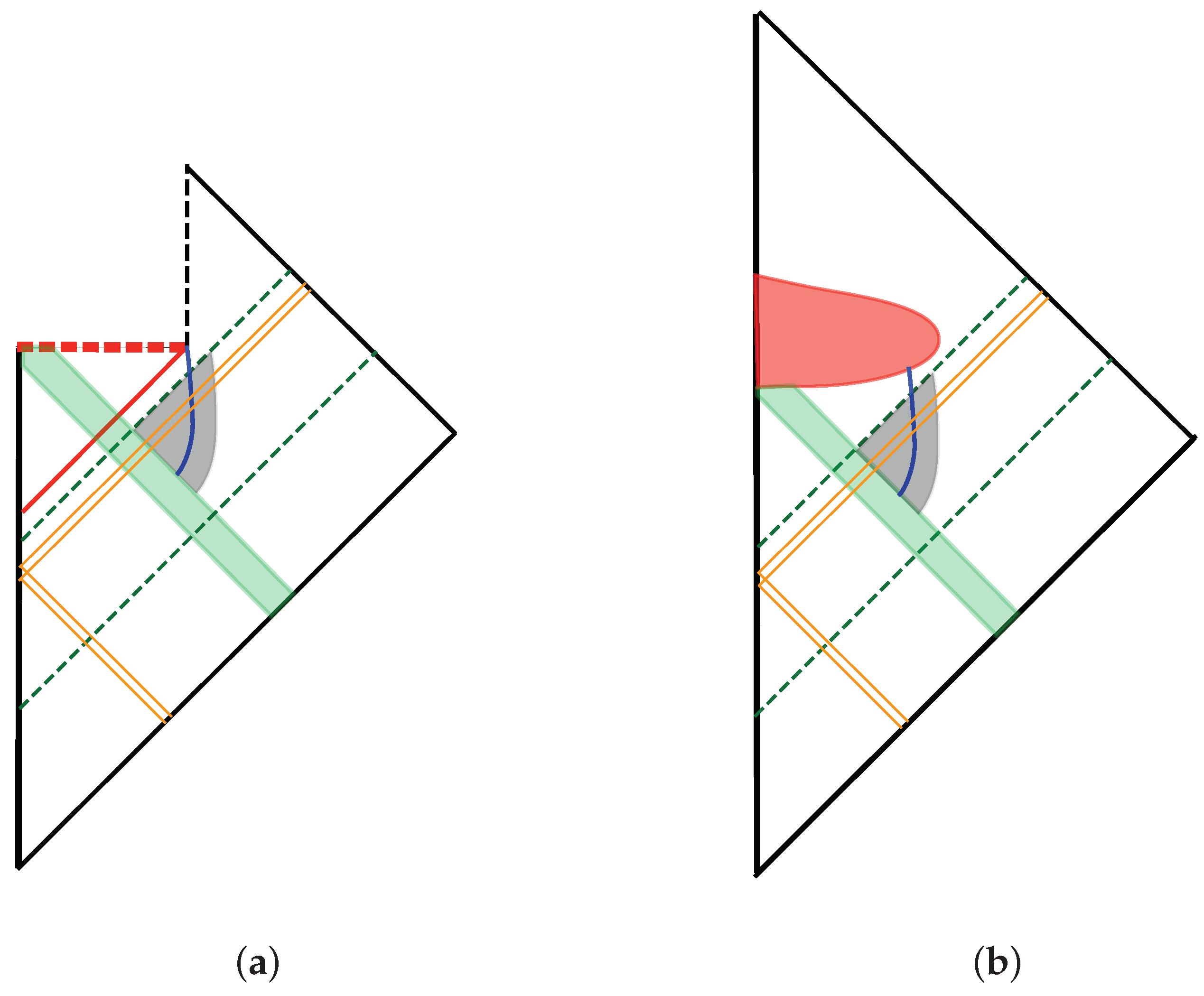
For the conventional model, the Penrose diagram of the time-dependent geometry (including the back reaction of the vacuum energy–momentum tensor) is given in Figure 1a4. The apparent horizon becomes time-like due to the quantum effect. If the space-like singularity at the origin is resolved by a UV-complete theory of quantum gravity, the Penrose diagram could be modified as Figure 1b.
In Figure 1a,b, we show two light rays (diagonal orange lines) as the causal past of two Hawking particles detected at future infinities. Regardless of whether there is an event horizon, Hawking radiation appears whenever it is an exponential relation between the affine parameter for ingoing light rays at the infinite past and the affine parameter for outgoing rays at the infinite future [32,33,34].
We are concerned with the causal past of all Hawking radiation observed at large distances over a period of time (bounded by the diagonal green dash lines in Figure 1) through which the black-hole mass is reduced from an initial mass to a small fraction of it, but still large enough so that the effective theory is valid. In both Figure 1a,b, this region of interest lies completely outside the event horizon, so the event horizon and the singularity are both causally irrelevant to our study.
Following recent progresses [28,29,35], we give below the approximate solution to the semi-classical Einstein equation in the near-horizon region for an adiabatic process. It is characterized by two (generalized) time-dependent Schwarzschild radii and (see Equation (17) for their definitions)5. Both and agree with the classical Schwarzschild radius a in the limit .
2.1. Near-Horizon Region and Uneventful Condition
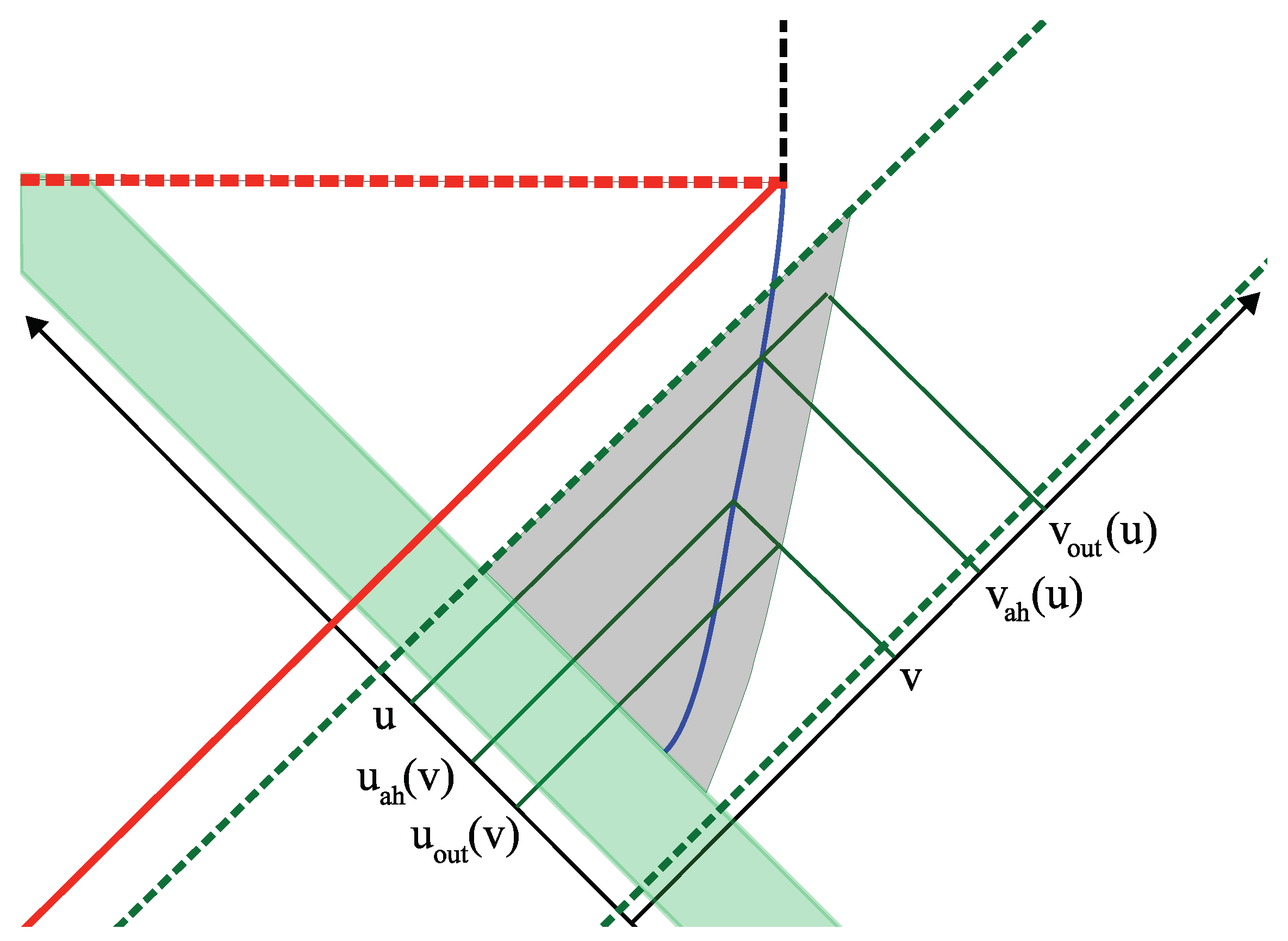
We start by reviewing the definition of the near-horizon region. Roughly speaking, it is defined to be the region near and inside the trapping horizon but outside the collapsing matter [29]. The surface of the collapsing matter is the inner boundary of the near-horizon region. The outer boundary is slightly outside the trapping horizon where the Schwarzschild approximation is valid. We will restrict our consideration to the early stage of black-hole evaporation when the trapping horizon is timelike in the near-horizon region (see Figure 2).
The definition of the outer boundary of the near-horizon region is clearly not unique. Nevertheless, since the quantum correction is small when , or equivalently, when according to Equation (3), it is reasonable to define it by the condition
where is the u-coordinate of the outer-boundary of the near-horizon region for a given value of v6. The number N should be so large that the Schwarzschild metric with the Schwarzschild radius is a good approximation around the outer boundary, but so small that the approximation (20) given below is good. (This range of N exists because the second condition only requires .) For a given value of u, the v-coordinate of the outer boundary of the near-horizon region will be denoted by . It should be the inverse function of : .
In the conventional model of black holes, the horizon is assumed to be “uneventful” [40,41,42,43,44]. This means that the vacuum energy–momentum tensor is not larger than for freely falling observers comoving with the collapsing matter. After the coordinate transformation to the light-cone coordinates , the conditions for uneventful horizons are given by [41,42]
This can be computed either by solving the geodesic equation for freely falling observers, or by computing the transformation factor between the coordinate u and the light-cone coordinate U suitable for the comoving observers (see Equation (54)).
The component (6) is nearly vanishing around the horizon because there, otherwise there would be a huge outgoing energy flux for observers comoving with the collapsing matter7. On the other hand, in the large distance limit where , approaches , corresponding to Hawking radiation at large distances, while in the asymptotically flat region, so the energy of the system must decrease. This means that the ingoing energy flux must be negative around the horizon for energy conservation. This negative ingoing energy is also the necessary condition for the appearance of a time-like trapping horizon (see, e.g., Ref. [35]). The outer boundary of the near-horizon region, which stays outside the trapping horizon, is also time-like. Hence, any point inside the trapping horizon satisfies
where and are the v and u coordinates of the trapping horizon at given u or v, respectively (see Figure 2).
In this paper, we will only consider the range of near-horizon region in which
For our conclusion about the breakdown of the effective field theory, we will only need the knowledge of the spacetime geometry in a much smaller neighborhood.
The energy–momentum tensor (6)–(9) for an uneventful horizon corresponds to the Unruh vacuum and is often viewed as an implication of the equivalence principle. However, we will see in Section 3 that an uneventful horizon always evolves into an eventful horizon at a later time for a generic effective theory soon after the collapsing matter enters the near-horizon region.
2.2. Solution of
In this subsection, we review the solution of in the metric (2) [28,29]. Two of the semi-classical Einstein equations and can be linearly superposed as [29]
where is defined by
For the Schwarzschild solution (3) and (4), becomes
in the near-horizon region.
We shall carry out our perturbative calculation in the double expansion of and . The red-shift factor is of around the trapping horizon, but gets exponentially smaller as one goes deeper into the near-horizon region (see Equations (13) and (14) above and Equation (20) below). With more focus on the deeper part of the near-horizon region, every quantity is first expanded in powers of , and then the coefficients of each term in powers of .
We expand as
where , , , etc. At the leading order, Equation (12) indicates
where we have used Equations (7) and (9) to estimate and .
Equation (16) can be easily solved by for two arbitrary functions and . Without loss of generality, we can define and by
so that
Comparing Equation (18) with the Schwarzschild case (14), we can see that and should be interpreted as generalizations of the notion of Schwarzschild radius for the dynamical solution. Roughly speaking, one may interpret as the Schwarzschild radius observed at the outer boundary of the near-horizon region along an infinitesimal slice from u to , and the Schwarzschild radius observed at the outer boundary along an infinitesimal slice from v to . (As the Schwarzschild metric is static, the Schwarzschild radius can be determined on a single slice of the spacetime. However, in the dynamical case, choosing a fixed u or a fixed v gives different geometries and thus different Schwarzschild radii.) See Ref. [29] for more discussion. At the leading order, agrees with the mass parameter in the special case of the ingoing Vaidya metric (see Appendix A). In the classical limit , both and approach the Schwarzschild radius a.
More precisely, since is independent of v, it can be identified with at the outer boundary of the near-horizon region (where the Schwarzschild solution is a good approximation). Similarly, is independent of u and it can also be determined this way. We can think of and as the Schwarzschild radii for the best fit of the Schwarzschild metric on constant-u and constant-v slices in a small neighborhood around the boundary of the near-horizon region. For a larger N (see Equation (5)), the Schwarzschild approximation is better at the outer boundary of the near-horizon region, hence there should be a smaller difference between and . In Appendix B, we derive the relation
between and at the boundary of the near-horizon region. The functional forms of and are determined by differential Equations (36) and (38) to be derived below.
It is then deduced from Equations (13), (15) and (18) that the solution of can be approximated by [29]
where and for an arbitrary reference point in the near-horizon region. For given u, since inside the near-horizon region (10), Equation (20) implies that , where can be estimated by the Schwarzschild approximation (3) to be , using Equation (5). Due to the exponential form of (20), the value of C is exponentially smaller as we move deeper inside the near-horizon region, i.e., for larger or larger .
2.3. Solution of
The solution of in the metric (2) can be readily derived using the solution of (20). We start by estimating the orders of magnitude of and . From the definition of the Einstein tensor for the metric (2):
the semi-classical Einstein equation and Equation (6), we derive
which can be integrated as
In this expression, we can choose so that is located on the outer boundary of the near-horizon region. The values of and can thus be estimated in the Schwarzschild approximation according to Equations (3) and (4), so the 2nd term in Equation (23) is of . One can use (20) to check that the first term in Equation (23) is much smaller than the 2nd term (see Appendix C). Thus, we find
In a similar manner as Appendix C, we can use (20) again to derive from and Equation (8) that
where we chose so that the reference point is located on the trapping horizon, and used the condition on the trapping horizon.
As the linear combination (12) of the semi-classical Einstein equations and is already satisfied by (20), only one more independent linear combination of them is needed. We choose to look at
Using Equations (7), (20), (24) and (25) to estimate the order of magnitude of each term in this equation, we find it to be dominated by the two terms and , so that
To integrate this, we suppose that the black hole evaporates in the time scale of as usual [4,5]. Hence, the u and v derivatives of and introduce additional factors of because the two radii are approximately the Schwarzschild radius. In addition, from Equations (24) and (25), the u and v derivatives of lead to extra factors of . On the other hand, with given by Equation (20), its u and v derivatives produce only factors of and , respectively. Thus, the functions , , and are approximately constant in comparison with , and Equation (27) can be solved by
for arbitrary functions and . However, comparing the first Equation (28) with Equation (24), we see that has to vanish, because a function of u cannot go to 0 as fast as in the limit . According to Equation (25), we find .
The consistent solution to the two equations above is
where the function can be determined as follows. First, in the classical limit, (3) can be rewritten as near , which resembles Equation (30). Since both and coincide with the Schwarzschild radius a in the classical limit, we have in the limit as well. Therefore, turning on the quantum effect, we expect to be approximately equal to . To estimate the order of magnitude of the difference , we plug the solution (30) into the condition (5) on the outer boundary of the near-horizon region for . Then, we find the relation
where we used Equations (3) and (5) to evaluate . Using Equation (31) in Equation (30), we find
in the near-horizon region.
Let us now determine the time-evolution of the functions and . Plugging Equations (20) and (32) back into the semi-classical Einstein equations (with Equation (21)), we can check that this equation is trivially satisfied at the leading order in the expansion and does not impose any constraint on . Similarly, we can see that gives
As the left-hand side of this equation is u-independent, is u-independent at the leading order in the near-horizon region. Recall the uneventful condition (8) that must be negative and of . It can be expressed as
for some parameter .
Now, we consider an adiabatic process [45] of Hawking radiation for which . Equation (34) then becomes
which determines the functional form of . The function is approximately equal to at due to Equation (19), so
where we used Equation (A10). Using Equation (19) on the right-hand side of Equation (36), we find
2.4. Near-Horizon Geometry
The solution for C (20) can now be further simplified using the solution for r (32) as
This and the solution of given by Equation (32) define the metric (2) for the geometry of the near-horizon region, with , satisfying Equations (36) and (38).
In the following, we will also need the Christoffel symbol of the metric (2):
with other components vanishing.
Finally, note that the characteristic length scale for all curvature invariants is still , e.g.,
where are only summed over the reduced 2D spacetime indices . As we will see below, nevertheless, the metric (32) and (39) together with the quantum effect of non-renormalizable operators lead to a non-trivial physical effect.
3. Breakdown of Effective Theory
For the low-energy effective theory of, say, a 4D massless scalar field , we have an action
with a Lagrangian density given as a -expansion:
(Assuming the symmetry , we omit terms of odd powers of for simplicity.) The dimensionless parameters are the coupling constants in a perturbation theory. Higher-dimensional terms are suppressed by higher powers of .
For a given physical state, it is normally assumed that all higher-dimensional (non-renormalizable) interactions, which are suppressed by powers of , only have negligible contributions to its time evolution. We will show below that, since the effective-field-theoretic derivation of Hawking radiation involves high-frequency modes of quantum fluctuations, there are in fact higher-dimensional operators in the effective Lagrangian (43) that contribute to large probability amplitudes of particle creation from the Unruh vacuum in the near-horizon region. We will see that this particle creation makes the uneventful horizon “eventful” or even “dramatic”.
3.1. Free-Field Quantization in the Near-Horizon Region
In this subsection, we introduce the quantum-field-theoretic formulation for the computation of the amplitudes mentioned above. It is essentially the same as the standard formulation for the derivation of Hawking radiation (see, e.g., Ref. [46]). The difference is that we shall consider the background geometry given in Section 2, instead of the static Schwarzschild background.
For a massless scalar field in the near-horizon region, we shall focus on its fluctuation modes with spherical symmetry. It is convenient to define
for the s-wave modes. For the metric (2), the free-field equation is equivalent to
According to Equations (27), (31) and (32), it becomes
in the near-horizon region. The free-field equation is thus well approximated by
deep inside the near-horizon region where C is exponentially small. Therefore, the general solution there is given by
Here, and are arbitrary functions of u and v, respectively. The creation and annihilation operators and satisfy
with the rest of the commutators vanishing.
In principle, we can use any functions and as the outgoing and ingoing light-cone coordinates. We shall choose the light-cone coordinates U and V so that the vacuum defined by
is the Minkowski vacuum of the infinite past before the gravitational collapse starts. This is the vacuum which evolves into Hawking radiation at large distances after it falls in from the past infinity, passes the origin, and then moves out [4,5]. We assume that this vacuum is the quantum state of the near-horizon region. It is equivalent to the Unruh vacuum—the vacuum state for freely falling observers at an uneventful horizon [47].
The relation between the coordinates U and u can be derived easily by considering the special case when the collapsing matter is a spherical thin shell at the speed of light, and identifying U with the retarded light-cone coordinate of the flat Minkowski spacetime inside the collapsing shell [40,48] as follows:8. The trajectory of the areal radius of the thin shell (where is the v-coordinate of the thin shell) satisfies
where we used in the flat space. It also satisfies
following Equations (32), (38) and (39). The two equations above imply
and hence the conditions (6)–(9) simply mean that .
We decompose the field (49) into the outgoing and ingoing modes. In the near-horizon region, the outgoing modes can be expanded in two bases:
The two expressions above are related by the coordinate transformation (54) and the creation and annihilation operators satisfy
They are related to via a Bogoliubov transformation
For the vacuum state defined by Equation (51), it is natural to define a 1-particle state
On the other hand, we also consider the 1-particle state
which is a superposition of the 1-particle states .
In the calculation below, we will need to evaluate the quantity , and hence we have to estimate the matrix appearing in Equation (62). As we will see, only a short time scale is relevant to our calculation below (see Equation (100)). Within this time scale, the black-hole mass does not change much so that remains roughly the same value that we will simply denote by a. Therefore, from Equations (38), (39) and (54), we have approximately
for an arbitrary constant , and is determined by Equation (54) to be
The Bogoliubov coefficients can be approximated by9
One then deduces from Equations (65) and (66) that
The normalization factor defined in Equation (62) is fixed by the condition
(following Equations (62), (66), (67) and (69)) to be
Then, we find
In Equation (51), we have introduced the coordinates as the light-cone coordinates used to define the Minkowski vacuum of the infinite past . Therefore, it is natural to identify the V-coordinate in the same approximation scheme as
so that we have
which leads to
This means that the coordinates are those of a freely falling observer who describes the spacetime locally as flat. Note that the coordinates take essentially the same form as the usual Kruskal coordinates. They play the role of the Kruskal coordinates in the dynamical spacetime.
For the ingoing modes, we have
and there are counterparts of the equations shown above for the outgoing modes. In particular, we can define the 1-particle states
However, we will not need the operators , defined with respect to the light-cone coordinates for the ingoing modes.
3.2. Transition Amplitude
In general, the effective Lagrangian (44) includes all local invariants. As examples, we consider a class of higher-dimensional, higher-derivative local observables of dimension :
where . The fields , , and are all massless scalars, and all equations for in Section 3.1 apply to , and . (The calculation below will be essentially the same if .)
Due to the dynamical background, this operator (77) introduces a time-dependent perturbation to the free field theory. The corresponding interaction term in the action (43) is
where is a coupling constant of . We shall consider its matrix element
integrated over a spacetime region , where is the Unruh vacuum and is a multi-particle state to be defined below.
For space (t is a time coordinate), the matrix element (79) can be interpreted as the transition amplitude from the initial state at to the final state at in the first-order time-dependent perturbation theory. We will show below that becomes exponentially large when the collapsing matter enters deeply inside the near-horizon region.
One might naively think that such a transition amplitude must be small since the initial state is the Unruh vacuum. As the typical length scale is for the small curvature (42), one expects that is by dimensional analysis. However, it turns out that becomes large as a joint effect of the peculiar geometry in the near-horizon region and the quantum fluctuation of the matter field.
The Hilbert space of the perturbative quantum field theory is the tensor product of the Fock spaces of the three fields , and . The initial state is the tensor product of the Unruh vacuum for each field,
The final state of interest is of the form
Here, is the superposition (62) of outgoing modes of , the k-particle state as a generalization of the 1-particle state (76) for the ingoing modes of , and the l-particle state of the ingoing modes of , respectively.
We shall choose
for the state . Notice that the prediction of the spectrum of Hawking radiation relies on a field-theoretic calculation of . If the state is not well-defined in the low-energy effective theory at least for , our understanding of Hawking radiation would be reduced to almost nothing. This state must be allowed in the effective theory; otherwise, the existence of Hawking radiation would be dubious.
On the other hand, the values of and will not play an important role in showing the matrix element (79) to be large. We shall simply choose
for simplicity.
Due to the s-wave reduction, all the spacetime indices are either u or v, and each factor of contributes a factor of . The covariant derivatives , involve derivatives , , which contribute factors of frequencies . Hence, the transition amplitude is the integral of a polynomial in , apart from an overall factor including . To show that the transition amplitude (79) is large, it is sufficient to focus on a term with given powers of , as they are independent free parameters. We shall focus on the terms with the largest power of but independent of . It is
The expression (84) for the transition amplitude tells us that the integral over is dominated by the contribution of the region where is large and C is small. On the other hand, it is unclear why a small conformal factor C, which has no particular local meaning for a freely falling observer, leads to a large transition amplitude. To understand the reason why the transition amplitude is large from the viewpoint of freely falling observers, we will rewrite this expression (84) in the next subsection in terms of the coordinates suitable for freely falling observers.
3.3. Comments on the Amplitude
We study here the properties of the amplitude (84) and explain the strategy of its evaluation for the next subsection.
3.3.1. Amplitudes in the Static Background
Before we estimate (84) for the dynamical background, we check that it vanishes for any static background, including the Schwarzschild metric. Let t be the time coordinate with translation symmetry, the functions C, r, and the Christoffel symbol are all independent of t. The only t-dependence in is thus the exponential factor , so we have
for space. The transition amplitude is non-zero as an artifact of the boundaries at and . It vanishes, for instance, if is quantized to satisfy the periodic boundary condition. Hence, unless the time-dependence of the dynamical background is taken into account, the transition amplitude vanishes for suitable boundary conditions. Note that, if , it means that particles (and hence their energies) are created out of the vacuum in ; is simply a consequence of energy conservation in the region with time-translation symmetry.
There are at least two origins for time dependence: (a) the collapsing matter that results in the black hole, and (b) the time-dependent geometry of the slowly evaporating black hole. We will see that either one is sufficient to result in a large amplitude .
3.3.2. Large Amplitudes in Dynamical Background
When the back-reaction of Hawking radiation is included, the factor
in the transition amplitude (84) has no time-translation symmetry, so its integral with the phase is in general non-zero.
Naively, even though (84) is no longer exactly 0, one might still expect that it is negligible due to the overall factor . However, this factor can be compensated by in Equation (86), since the conformal factor C can be arbitrarily close to 0 deep inside the near-horizon region. According to the solution of C (39), a displacement of u or v by a small amount is enough to compensate a factor of .
The claim that the matrix element can become large due to a small C is unsettling because the appearance of the arbitrarily small conformal factor C relies on the choice of the coordinate system. If we use the Kruskal coordinate (given by Equations (63) and (72)), the metric becomes locally Equation (74); the conformal factor is 1. A natural question is then: How can the amplitude become large? As the operator (77) is by definition a scalar, its integral over a given region of spacetime is independent of the choice of coordinates. To understand the physics better, let us first answer this question by analyzing in terms of .
For the locally flat metric (74), we have and . When we rewrite the amplitude (84) in terms of the coordinate system, it becomes
where
To derive this expression, we have used Equations (80) and (81) for the states , , Equation (77) for the operator , and Equations (50), (55), (61), (62), (65), (66) and (83) to evaluate the matrix element. This is simply Equation (84) written in terms of the Kruskal coordinates.
Indeed, the expression (87) does not explicitly involve any exponentially growing factor. To see how the factor in Equation (84) is hidden in the expression above, we should carry out the integration over . The -integral of the form
in Equation (87) (with ) can be evaluated using the saddle point approximation. The saddle point is
where we have used Equation (63). It is important to note that is large when the blue-shift factor is large.
The integral over in Equation (87) is thus approximately
up to a factor of .
On the other hand, the factor appears from
in Equation (87), where . Thus, in Equation (92) (for ) and in Equation (93) produce the hidden factor according to Equation (73). This explains how the large factor arises in the calculation in terms of the -coordinates10.
Strictly speaking, the region of integration needs to be infinitely large so that the Fourier transform with respect to is well defined. For a finite , we should use a suitable complete basis of functions in . A simple example is when is a rectangular region with periodic boundary conditions such that can be used as the basis, but is discretized (see, e.g., Equation (A22)). In this case, we should first integrate over to find (89), assuming that is properly discretized, and then replace in Equation (87) by a sum over discretized values of . For a sufficiently large region , the sum over should be well approximated by the integral, so we expect that the conclusion above for infinite remains qualitatively correct for a finite . In Appendix D, we consider the discretization of for a finite region and carry out the explicit calculation of the transition amplitude to demonstrate the general expectation described above.
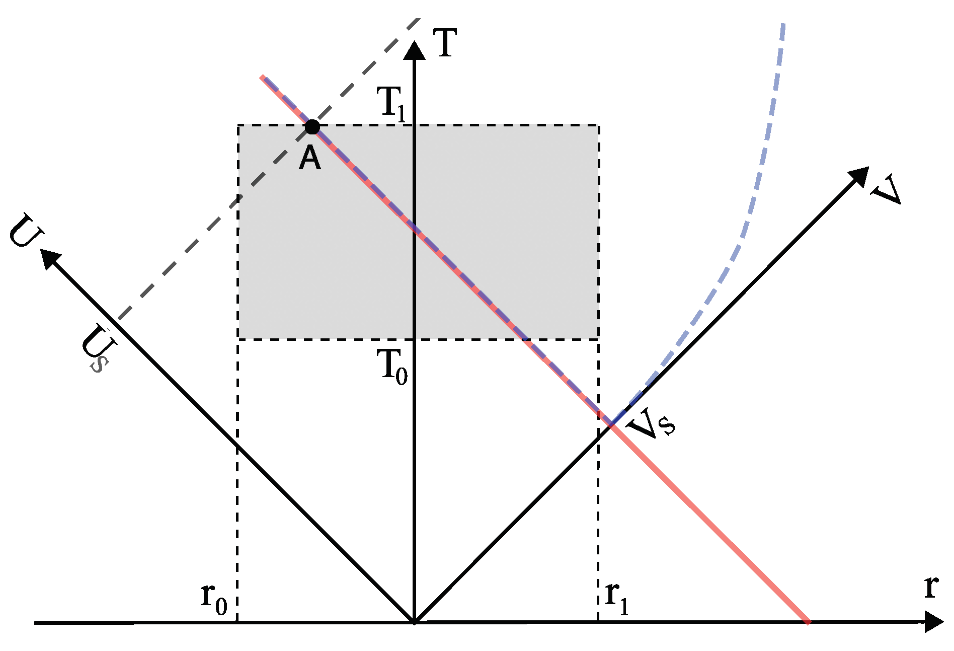
3.4. Example: Thin Shell and
To demonstrate explicitly that the magnitude of the amplitude (87) becomes large as the collapsing matter falls further inside the near-horizon region (so that the conformal factor C becomes small), we study a simple example here. We consider a thin shell collapsing at the speed of light along the curve and investigate a special class of higher-derivative interactions
This is the case of (77) with for and , and we assume .
In terms of the time coordinate T defined by
we choose to be a rectangle which covers a large space (see Figure 3). It can be divided into the following four parts: (i) the space outside the near-horizon region ( and ), (ii) the near-horizon region ( and ), (iii) the thin shell (), and (iv) the flat space inside the shell ().
In Appendix D, we evaluate the order of magnitude of as
up to a factor of . The dominant contribution comes from the neighborhood of the point A in Figure 3, where A is the corner with the maximal value of u and minimal value of v along the trajectory of the collapsing shell in (recall Equation (10) and see Figure 3). This implies that the shape of the region is not important11.
We note that the conformal factor in scales by a factor of under a shift in by . It implies that the amplitude (96) is exponentially larger when the collapsing shell is deeper inside the near-horizon region.
is the time duration of the region for a distant observer, and we will be interested in a duration of time of the order of the scrambling time, [24]. Here, we assume that
Here, we have chosen the reference point to be located on the trapping horizon so that
which comes from Equations (3) and (5). Therefore, the matrix element is larger than when
For example, let us take the reference point to be the point where the shell crosses the trapping horizon (the trapping horizon emerges at this moment ) so that . Then, the matrix element becomes larger than after an elapse of time of the same order of magnitude as the scrambling time . (This is consistent with the range of the near-horizon region (10)).
A large matrix element implies a large transition amplitude from (80) to (81). As the thin shell falls further deep under the apparent horizon, the energy flux of the created outgoing particles in grows exponentially. This can be identified with the firewall [17,20,21] because the saddle-point frequency is trans-Planckian with respect to comoving observers. (There will be more discussion on this in the next subsection.) According to Equation (100), it should appear within the scrambling time after the shell enters the apparent horizon. In fact, we will see below that the transition amplitudes become large for many other higher-derivative interactions even before the condition (100) is met.
Finally, we discuss the contribution of the region within the collapsing matter to the amplitude . In the case above, the region within the thin shell is the subspace , and it has no contribution to Equation (96) because the delta function does not appear (see Appendix D). For a generic matter distribution, however, a higher energy density is expected to induce a larger transition amplitude for a generic higher-derivative operator. However, since the matter distribution is arbitrary, its contribution to the amplitude is under little constraint.
On the other hand, even if the prefactor in Equation (98) is much smaller (say, by a factor of as it would be if only the contribution of the time dependence of the near-horizon geometry outside the collapsing shell is included, see Appendix D), the amplitude still becomes large within a period of time of the same order of magnitude as the scrambling time. For this reason, we shall focus on the contribution of the vacuum geometry outside the collapsing shell in the near-horizon region. The conclusion about the scrambling time should be valid for generic matter configuration13.
3.5. Firewall
Now, we consider another class of operators different from the example above. We show that the matrix element becomes huge at the moment when the collapsing matter enters the near-horizon region, and this corresponds to the firewall.
Consider the operators
which is with , and . ( and n is even.) The corresponding matrix element (87) is given by Equations (88) and (89) as
As we commented at the end of Section 3.4, when higher-derivatives of the quantum fields are involved, the contribution of the matter to the matrix element depends on the details of the matter configuration. To avoid this uncertainty, in this section, we will focus on the contribution of the near-horizon region, even though the contribution of the region occupied by the collapsing matter can be larger.
The derivation is essentially the same as that of Equation (96) in Appendix D, but only with the contribution of the near-horizon region taken into consideration.
For a reasonably long period of time (97) for the region from the viewpoint of a distant observer (which is an extremely short time for a freely falling observer), the amplitude is larger than as long as
This is a smaller lower bound than Equation (100) for but still the same order of magnitude as the scrambling time for finite n.
The final state for the exponentially increasing transition amplitude includes the outgoing mode (62), which is a superposition of 1-particle states for freely moving observers. For comoving observers, the dominant frequency of these 1-particle states is the saddle point (91) with the magnitude
which is trans-Planckian at well before Equation (105) is satisfied. Hence, the large matrix elements imply the presence of a firewall as a flux of trans-Planckian particles in the comoving frame.
Before the effective theory breaks down, there are particle creations with exponentially increasing probability, although the prediction of a firewall as a Planckian energy flux is not reliable. Depending on the UV-theory (or some of the coupling constants at large n), the energy flux of the created particles may or may not become Planckian before the effective theory breaks down. It is possible that the UV theory admits a new effective theory that will become appropriate to describe what happens afterwards.
3.6. Viewpoint of Freely Falling Observers
The saddle point approximation (91) shows that the matrix element is dominated by contributions of trans-Planckian modes . The physical reason behind this is clear. The Hawking radiation is dominated by modes with frequencies at large distances. Tracing these wave packets backwards to the near-horizon region, they are blue-shifted to trans-Planckian frequencies .
If the trans-Planckian modes are removed from the effective theory, the matrix elements would not become large, but it also implies that there would be no Hawking radiation either. This is reminiscent of the trans-Planckian problem [50].
Note that we have chosen to consider the 1-particle state in the final state because our understanding of the spectrum of Hawking radiation relies on the quantity , which demands that the state be well-defined. If the amplitude is considered ill-defined because of its involvement with the trans-Planckian modes, the spectrum of Hawking radiation is also ill-defined. While the derivation of Hawking radiation assumes that the free-field approximation is good, the matrix elements can be interpreted as perturbative corrections to the calculation of the spectrum of Hawking radiation by higher-derivative interactions. Large means that Hawking radiation is largely corrected.
Therefore, assuming Hawking radiation and the uneventful horizon, we cannot avoid the large matrix elements, leading to the breakdown of the low-energy effective theory. On the other hand, it is possible that, in a self-consistent model, there is a moderately large energy flux around the horizon (so that it is not uneventful but also no trans-Planckian modes) so that a low-energy effective description is still valid [51]. Alternatively, another logical possibility is that Hawking radiation stops while the horizon remains free of the Planckian firewall. More rigorously, what we have shown is the incompatibility between Hawking radiation and uneventful horizon in the effective-field-theoretic description.
Incidentally, as an effort to resolve the trans-Planckian problem, there have been proposals of alternative derivations of Hawking radiation which assume non-relativistic dispersion relations such that the energy is bounded from above to be cis-Planckian [52,53,54]. They reproduce the same spectrum of Hawking radiation, but this does not completely resolve the trans-Planckian problem [55] as the wave numbers can still be arbitrarily large. In the context of this paper, it is reasonable to expect that, since the wave number is still allowed to go to infinity, there are higher-dimensional operators (which are no longer required to be Lorentz-invariant) that produce large transition amplitudes, and the low-energy effective theory still breaks down. While this remains to be rigorously proven, what we have shown is at least that, for relativistic low-energy effective theories, Hawking radiation (which necessarily includes trans-Planckian modes) is in conflict with the assumption of an uneventful horizon.
Notice that one should not simply dismiss quantum modes with as an attempt to solve the trans-Planckian problem. There are infinitely many freely falling frames at different velocities. They are related to one another via a local Lorentz boost
for a relative velocity w. A constraint like has no locally invariant meaning, as it can always be violated for any non-zero frequency after a boost. In contrast, our calculation is invariant under general coordinate transformations.
Our work distinguishes itself from previous discussions on the trans-Planckian problem in two clear aspects. First, we focus only on locally Lorentz-invariant quantities, acknowledging the fact that a trans-Planckian frequency can be cis-Planckian to another observer. Second, the time-dependence of the geometry (due to the collapsing shell and the evaporation—including the back-reaction of the vacuum energy–momentum tensor) is mostly ignored in previous works on the trans-Planckian problem, but it is absolutely crucial for our conclusion, as explained above in Section 3.3.1.
The choice of a freely falling frame is related to the interpretation of the origin of the large matrix elements. In our calculations, the origin of the largeness of the matrix element is the largeness of . Equivalently, according to Equation (73), it is the largeness of in the saddle point (91) and/or in the derivative . Which one, or , is large? The answer depends on the choice of the freely falling frame14. A local Lorentz boost Equation (107) changes and simultaneously, making one bigger and the other smaller.
A large implies a large dominant frequency (91) of the 1-particle states for freely falling observers, and a large means a large V-derivative of the areal radius (30), i.e., a fast deformation of the background geometry. (The magnitude of is as small as , but can be larger if is large.) The collision between the outgoing quantum fluctuation and the ingoing geometric deformation defines a Lorentz invariant energy scale. When this Lorentz invariant becomes too large, the effective theory breaks down.
4. Discussion and Conclusions
In this work, we showed that Hawking radiation is incompatible with the uneventful horizon. Assuming the validity of the effective-theoretic derivation of Hawking radiation, the higher-dimensional operators in the effective action change the time evolution of the Unruh vacuum in the near-horizon region of the dynamical black hole so that it evolves into an excited state with many high-energy particles for freely falling observers. The uneventful horizon transitions to an eventful horizon (the firewall), and ultimately the effective theory breaks down.
We emphasize that we have only used the semi-classical Einstein equation and the conventional formulation of the quantum field theory for the matter field. The only novel ingredients are (i) the explicit solution of the metric in the near-horizon region and (ii) the consideration of higher-dimensional operators in the effective theory.
For the first item (i), we used the metric given by Equations (20) and (32) as a solution to the semi-classical Einstein equation for the energy–momentum tensor (6)–(9) of the uneventful horizon. As a result of the negative ingoing energy flux , the trapping horizon is time-like [35], with the causal structure of the near-horizon region satisfying Equation (10). This is crucial for the exponential form of the red-shift factor to lead to the exponentially large transition amplitudes after the matter enters the near-horizon region.
We also emphasize the importance of the dynamical nature of the background geometry. Had we used the static Schwarzschild solution for the background geometry, the conformal factor would still have the exponential form, but the matrix elements would be negligible.
About the item (ii), we considered the quantum effect of the higher-dimensional operators (77) for . These are non-renormalizable operators that are normally ignored in the low-energy effective theory because they are suppressed by powers of . However, we found that these operators induce large transition amplitudes related to the creation of particles from the Unruh vacuum, in contrast with renormalizable operators. A lot of the high-energy particles are created for freely falling observers, resulting in the firewall. This invalidates the conditions (6)–(9) for an uneventful horizon.
Note that no local curvature invariants of the dynamical background are found to be large in the near-horizon region. The high-energy events only arise from the higher-dimensional terms in the effective action, and their origin is a joint effect of the higher-derivative interactions and the peculiar geometry of the near-horizon region.
Assuming a persisting Hawking radiation, together with higher-dimensional operators, there is a firewall, and the equivalence principle is violated in the sense that a freely-falling observer sees particles with high energy. Indeed, the equivalence principle is in general violated by higher-derivative interactions. This has been shown for classical electromagnetism [56]. Although the equivalence principle is violated, general covariance, including the local Lorentz transformation (107), is preserved.
Until now, we have restricted our discussions to the standard application of a generic low-energy effective theory to the process of black-hole formation and evaporation, without assuming that there is no information loss. Our calculation shows that the uneventful horizon and Hawking radiation are incompatible beyond the scrambling time, hence the conventional model is incompatible with a generic effective theory. However, we have not yet commented much on how the information is preserved. If one carefully analyzes the information loss paradox, one finds that it involves two different questions. The first question is “How can the conventional model based on the low-energy effective theory be wrong?”. This paper is devoted to answering this question. The second question is “What is the new mechanism missing in the effective theory that avoids information loss?”. We have intentionally refrained ourselves from making concrete proposals about the answer to the second question, because we think it is conceptually important to distinguish these two questions. Nevertheless, let us briefly comment now on potential resolutions to the 2nd question below.
If there is a firewall, the trans-Planckian scattering between the firewall and the collapsing matter cannot be ignored. It is possible that, through such trans-Planckian scatterings, the information of the collapsing matter is transferred into the outgoing particles, and information is preserved. A priori, this process involves Planckian events that demands a theory of quantum gravity. However, an interesting proposal was made in Refs. [57,58], where, remarkably, only low-energy particles are needed to describe this unitary process through the proposal of the “anti-podal identification”.
Another possibility is that we abandon the assumption of uneventful horizon (6)–(9) from the beginning. It is then still possible that a consistent low-energy effective theory describes an evaporating black hole. A self-consistent scenario is perhaps one that would have no horizon or trapped region, such as the model proposed in Refs. [51,59,60] (see also [61,62,63,64,65,66,67]). It is also recently argued that a consistent quantum theory of gravity should always admit the VECRO [68], which will likely modify the conventional energy–momentum tensor.
To conclude, we have shown that Hawking radiation and uneventful horizon cannot coexist with each other over the scrambling time. The low-energy effective theory breaks down as a result of time evolution from the Unruh vacuum towards the firewall due to higher-derivative interactions. How information is preserved is still a problem, but it is no longer a paradox.
Author Contributions
All the authors have contributed to the research and the writing of the manuscript. All authors have read and agreed to the published version of the manuscript.
Funding
P.M.H. is supported in part by the Ministry of Science and Technology, R.O.C. and by National Taiwan University. Y.Y. is partially supported by the Japan Society of Promotion of Science (JSPS), Grants-in-Aid for Scientific Research (KAKENHI) Grant Nos. 21K13929, 18K13550 and 17H01148. Y.Y. is also partially supported by RIKEN iTHEMS Program.
Institutional Review Board Statement
Not applicable.
Informed Consent Statement
Not applicable.
Acknowledgments
We thank Hsin-Chia Cheng, Hsien-chung Kao, Hikaru Kawai, Samir Mathur, and Yoshinori Matsuo for valuable discussions. P.M.H. thanks iTHEMS at RIKEN, Tokyo University, and Kyoto University for their hospitality during his visits when this project was initiated.
Conflicts of Interest
The authors declare no conflict of interest.
Appendix A. Ingoing Vaidya Metric
We consider the ingoing Vaidya metric as an example to demonstrate the meanings of the generalized Schwarzschild radii and . The ingoing Vaidya metric
where is proportional to the mass parameter of the black hole, is a spherically symmetric solution to the Einstein equation for the energy–momentum tensor
with all other components (, etc.) vanishing. For , the energy–momentum tensor satisfies the uneventful-horizon condition (6)–(9), hence the metric (A1) is just a special case of the general solution (20), (32) in the near-horizon region.
To put the metric (A1) in the form of Equation (2), we plug into the metric (A1) and demand that it agrees with Equation (2). It is
which means that
It is then easy to check that the solution of r (33) satisfies both conditions above at the leading order of the -expansion, in which , via the identification
Therefore, can be identified with the Schwarzschild radius of the ingoing Vaidya metric at the leading order.
On the other hand, the parameter is not directly fixed by the ingoing Vaidya metric because the form of the metric (2) is invariant under a coordinate transformation . The u-coordinate in the solution (20), (33) has been chosen such that, on the outer-boundary of the near-horizon region, it agrees with the u coordinate used in the Schwarzschild solution (3), (4). This is realized in Equation (19), which relates to there.
Appendix B. Relation between a(u) and
Here, we derive the relation (19) between the Schwarzschild radii and on the outer boundary of the near-horizon region. Take the v-derivative of Equation (5), which defines the location of the outer boundary of the near-horizon region, we find
Use Equations (3)–(5) to estimate and as
Then, together with Equation (38), the equation above becomes
which implies that
assuming that .
Appendix C. Order-of-Magnitude of the First Term in Equation (23)
Using Equations (6), (20), and , the first term in Equation (23) can be estimated as
where we assumed that the range so that the Schwarzschild radius a remains the same order of magnitude. (This assumption is consistent with the range (11).) The integral above can then be estimated as
In the evaluation of Equation (23), we have taken so that lies on the outer boundary of the near-horizon region. Then, we can use Equations (3) and (5) to evaluate . Following Equation (A14), the first term in Equation (23) is estimated as
On the other hand, the second term in Equation (23) is of . Therefore, the first term is negligible in comparison.
Appendix D. Calculation of
We evaluate M here by using the expression (89) for :
We consider the spacetime region as shown in Figure 3. Equation (A17) includes all the contributions from the regions (i)–(iv).
As the areal radius r has different functional forms inside and outside the shell, the factor appearing in Equation (A17) is of the following form:
where is the V-coordinate of the collapsing thin null shell and () the areal radius inside (outside) the shell. The step function selects the region inside the shell, and that outside the shell.
In the flat space inside a collapsing shell, we have
where . The value of is fixed by the continuity of r across the thin shell when it is deep inside the near-horizon region, using Equations (63), (72) and (33).
According to Equation (A19), . We derive from Equations (19), (32), (36), (63), (72) and (73) as
in the near-horizon region. Using Equation (72), we see that on the shell at . On the other hand, becomes arbitrarily small deep inside the near-horizon region.
The step functions in Equation (A18) divide the integral (A17) into two parts:
is the contribution from the region (iv), and is that from the regions (i) and (ii). Note that there is no contribution from (iii) due to the absence of in Equation (A18).
Before evaluating the contributions inside and outside the collapsing shell to the transition amplitude, we note that the spacetime is divided into two parts here as and by a physical object—the null shell. This is in contrast with the calculation of matrix elements in which the spacetime is divided into two parts by the event horizon. Since the event horizon has no local physical meaning, it was found in Ref. [49] that the contributions of the two parts of the spacetime cancel to a large extent in the calculation of certain matrix elements.
On the other hand, in the near-horizon region, it is unlikely to have generic cancellation between and because only the region outside the shell depends on the mass. As we will see below, the large difference between and across the null shell in the near-horizon region leads to a significant contribution to the amplitude .
To define a complete basis of functions in this region, we impose the periodic boundary conditions in T for convenience (T is defined in Equation (95)). The frequency is thus quantized as
The integral over can be easily carried out using the following formula:
where we assumed that
This will be a good approximation because the integral over will be dominated by a trans-Planckian value with (82). We will apply this formula (A23) to integrals over the variables V and T below.
The shell is collapsing at the speed of light at , with the areal radius
assuming that for . Now, we evaluate using Equations (A17), (A18), (A19) and (A23), we find
Note that the 2nd term in the integral on the right-hand side has no contribution due to the condition (A22). Hence, using Equations (A22) and (A23) again, we obtain
where, in the 2nd last line, we used
for , and, in the last line, we have used as the typical order of magnitude on the shell.
Similarly, letting denote the upper bound of the V-integration corresponding to , we have, for ,
where is replaced by as an order-of-magnitude estimate, and we have used Equation (A20) (and the Taylor expansion of its n-th power) as well as Equation (A23). Here, the spacetime at is far away the near-horizon region, and the contribution is negligible due to compared to that from . The spacetime at is inside the near-horizon region, and Equation (A20) has been used. Using Equations (A22) and (A23) again for the integration over T, we find
where we used according to Equation (72)15.
Thus, is negligible in comparison with . The origin of this hierarchy is the large difference in inside and outside the shell mentioned above. If the shell is not in the near-horizon region, but far away from the horizon , and would be of the same order of magnitude and have the possibility of a large cancellation between them.
Plugging back into Equation (87), the integral should be replaced by the sum over with as
where is the U-coordinate of the collapsing shell at . In the expression above, we have assumed that . This is consistent with the consideration of a scrambling time for a distant observer.
Using the identity
and
where is the u-coordinate of the point , the transition amplitude (87) is found to be
up to a factor of .
One might suspect that the origin of the large amplitude is the -function energy density of the thin shell. A shell with a smooth energy density could in principle lead to a smaller , but, as mentioned above, even the contribution of the vacuum energy is sufficient to induce a large amplitude within the scrambling time. The conclusion is robust because of the exponential behavior of .
| 1 | |
| 2 | A “high-energy event” refers to a physical observable at an energy scale higher than the cutoff energy of the low-energy effective theory. |
| 3 | There is no clear inconsistency in a unitary evaporation without high-energy events [16] if there are no small particles like nuclei. However, we will show below that a firewall still arises under general assumptions. |
| 4 | |
| 5 | |
| 6 | It is equally natural to use the condition instead of Equation (5). This different choice would not make any essential difference in the discussion below. |
| 7 | |
| 8 | If the collapsing shell is not thin, it only introduces negligible corrections to the relation between U and u in the near-horizon region. |
| 9 | See, for example, Ref. [46]. |
| 10 | There may be other factors of C to a positive power in the calculation of the amplitude, but we will see that, generically, with a sufficiently large order of derivatives, the amplitude involves a negative power of C. |
| 11 | It was pointed out in Ref. [49] that a large matrix element is obtained (for an operator without higher derivatives) when only the space outside the event horizon is integrated over, but it is merely an artifact of the boundary condition at the event horizon, and this large contribution is cancelled by the space inside the event horizon. Here, we take to cover the four different regions (i)–(iv) to rule out the possibility that the matrix element becomes large due to an artificial boundary condition. |
| 12 | For large n, the amplitude is further enhanced by other factors in Equation (96). |
| 13 | The potential cancellation between the contribution from the time-dependent matter distribution and that from the time-dependent vacuum geometry generically requires fine tuning (see Appendix D for more discussion). |
| 14 | For a freely falling observer comoving with the collapsing matter, the v-coordinate of the observer in this frame is roughly constant. The coordinates suitable for the observer are given by Equations (63) and (72), and the transition amplitude increases with the retarded time u mostly due to the increase in rather than that in . |
| 15 |
References
- Hawking, S.W. Breakdown of Predictability in Gravitational Collapse. Phys. Rev. D 1976, 14, 2460. [Google Scholar] [CrossRef]
- Mathur, S.D. The Information paradox: A Pedagogical introduction. Class. Quant. Grav. 2009, 26, 224001. [Google Scholar] [CrossRef] [Green Version]
- Marolf, D. The Black Hole information problem: Past, present, and future. Rept. Prog. Phys. 2017, 80, 092001. [Google Scholar] [CrossRef] [PubMed]
- Hawking, S.W. Particle Creation by Black Holes. Commun. Math. Phys. 1975, 43, 199. [Google Scholar] [CrossRef]
- Hawking, S.W. Black Holes and Thermodynamics. Phys. Rev. D 1976, 13, 191. [Google Scholar] [CrossRef]
- Hawking, S.W. Information Preservation and Weather Forecasting for Black Holes. arXiv 2015, arXiv:1401.5761. [Google Scholar]
- Hawking, S.W. The Information Paradox for Black Holes. arXiv 2014, arXiv:1509.01147. [Google Scholar]
- Saini, A.; Stojkovic, D. Radiation from a collapsing object is manifestly unitary. Phys. Rev. Lett. 2015, 114, 111301. [Google Scholar] [CrossRef] [Green Version]
- Zhang, B.; Cai, Q.Y.; You, L.; Zhan, M.S. Hidden Messenger Revealed in Hawking Radiation: A Resolution to the Paradox of Black Hole Information Loss. Phys. Lett. B 2009, 675, 98. [Google Scholar] [CrossRef] [Green Version]
- Zhang, B.; Cai, Q.Y.; Zhan, M.S.; You, L. Entropy is Conserved in Hawking Radiation as Tunneling: A Revisit of the Black Hole Information Loss Paradox. Ann. Phys. 2011, 326, 350. [Google Scholar] [CrossRef] [Green Version]
- Zhang, B.; Cai, Q.Y.; Zhan, M.S.; You, L. Towards experimentally testing the paradox of black hole information loss. Phys. Rev. D 2013, 87, 044006. [Google Scholar] [CrossRef] [Green Version]
- Zhang, B.; Cai, Q.Y.; Zhan, M.S.; You, L. Information conservation is fundamental: Recovering the lost information in Hawking radiation. Int. J. Mod. Phys. D 2013, 22, 1341014. [Google Scholar] [CrossRef] [Green Version]
- Penington, G. Entanglement Wedge Reconstruction and the Information Paradox. J. High Energy Phys. 2020, 2020, 1–84. [Google Scholar] [CrossRef]
- Almheiri, A.; Engelhardt, N.; Marolf, D.; Maxfield, H. The entropy of bulk quantum fields and the entanglement wedge of an evaporating black hole. J. High Energy Phys. 2019, 1912, 63. [Google Scholar] [CrossRef] [Green Version]
- Almheiri, A.; Mahajan, R.; Maldacena, J.; Zhao, Y. The Page curve of Hawking radiation from semiclassical geometry. arXiv 2019, arXiv:1908.10996. [Google Scholar] [CrossRef] [Green Version]
- Hutchinson, J.; Stojkovic, D. Icezones instead of firewalls: Extended entanglement beyond the event horizon and unitary evaporation of a black hole. Class. Quant. Grav. 2016, 33, 135006. [Google Scholar] [CrossRef] [Green Version]
- Almheiri, A.; Marolf, D.; Polchinski, J.; Sully, J. Black Holes: Complementarity or Firewalls? J. High Energy Phys. 2013, 1302, 62. [Google Scholar] [CrossRef] [Green Version]
- Lunin, O.; Mathur, S.D. AdS/CFT duality and the black hole information paradox. Nucl. Phys. B 2002, 623, 342. [Google Scholar] [CrossRef] [Green Version]
- Lunin, O.; Mathur, S.D. Statistical interpretation of Bekenstein entropy for systems with a stretched horizon. Phys. Rev. Lett. 2002, 88, 211303. [Google Scholar] [CrossRef] [PubMed] [Green Version]
- Braunstein, S.L. Black hole entropy as entropy of entanglement, or it’s curtains for the equivalence principle. arXiv 2009, arXiv:0907.1190v1. [Google Scholar]
- Braunstein, S.L.; Pirandola, S.; Życzkowski, K. Better Late than Never: Information Retrieval from Black Holes. Phys. Rev. Lett. 2013, 110, 101301. [Google Scholar] [CrossRef] [PubMed]
- Dodelson, M.; Silverstein, E. String-theoretic breakdown of effective field theory near black hole horizons. Phys. Rev. D 2017, 96, 066010. [Google Scholar] [CrossRef] [Green Version]
- Weinberg, S. The Quantum Theory of Fields; Cambridge University Press: Cambridge, UK, 1995; Volume 1. [Google Scholar]
- Sekino, Y.; Susskind, L. Fast Scramblers. J. High Energy Phys. 2008, 10, 65. [Google Scholar] [CrossRef] [Green Version]
- Nurmagambetov, A.J.; Park, I.Y. Quantum-induced trans-Planckian energy near horizon. J. High Energy Phys. 2018, 5, 167. [Google Scholar] [CrossRef] [Green Version]
- Nurmagambetov, A.J.; Park, I.Y. Quantum-gravitational trans-Planckian energy of a time-dependent black hole. Symmetry 2019, 11, 1303. [Google Scholar] [CrossRef] [Green Version]
- Nurmagambetov, A.J.; Park, I.Y. Quantum-gravitational trans-Planckian radiation by a rotating black hole. arXiv 2020, arXiv:2007.06070. [Google Scholar]
- Ho, P.M.; Matsuo, Y.; Yokokura, Y. An Analytic Description of Semi-Classical Black-Hole Geometry. arXiv 2020, arXiv:1912.12855. [Google Scholar]
- Ho, P.M.; Matsuo, Y.; Yokokura, Y. Distance between collapsing matter and trapping horizon in evaporating black holes. arXiv 2019, arXiv:1912.12863. [Google Scholar]
- Hiscock, W.A. Models of Evaporating Black Holes. {II}. Effects of the Outgoing Created Radiation. Phys. Rev. D 1981, 23, 2823–2827. [Google Scholar] [CrossRef]
- Ashtekar, A. Black Hole evaporation: A Perspective from Loop Quantum Gravity. Universe 2020, 6, 21. [Google Scholar] [CrossRef] [Green Version]
- Visser, M. Essential and inessential features of Hawking radiation. Int. J. Mod. Phys. D 2003, 12, 649–661. [Google Scholar] [CrossRef] [Green Version]
- Barcelo, C.; Liberati, S.; Sonego, S.; Visser, M. Quasi-particle creation by analogue black holes. Class. Quant. Grav. 2006, 23, 5341–5366. [Google Scholar] [CrossRef]
- Barcelo, C.; Liberati, S.; Sonego, S.; Visser, M. Hawking-like radiation does not require a trapped region. Phys. Rev. Lett. 2006, 97, 171301. [Google Scholar] [CrossRef] [Green Version]
- Ho, P.M.; Matsuo, Y. Trapping Horizon and Negative Energy. J. High Energy Phys. 2019, 1906, 57. [Google Scholar] [CrossRef] [Green Version]
- Ho, P.M.; Matsuo, Y. Static Black Holes With Back Reaction From Vacuum Energy. Class. Quant. Grav. 2018, 35, 065012. [Google Scholar] [CrossRef] [Green Version]
- Ho, P.M.; Matsuo, Y. Static Black Hole and Vacuum Energy: Thin Shell and Incompressible Fluid. J. High Energy Phys. 2018, 1803, 96. [Google Scholar] [CrossRef]
- Ho, P.M.; Matsuo, Y. On the Near-Horizon Geometry of an Evaporating Black Hole. J. High Energy Phys. 2018, 1807, 47. [Google Scholar] [CrossRef] [Green Version]
- Ho, P.M.; Kawai, H.; Matsuo, Y.; Yokokura, Y. Back Reaction of 4D Conformal Fields on Static Geometry. J. High Energy Phys. 2018, 1811, 56. [Google Scholar] [CrossRef] [Green Version]
- Davies, P.; Fulling, S.; Unruh, W. Energy Momentum Tensor Near an Evaporating Black Hole. Phys. Rev. D 1976, 13, 2720–2723. [Google Scholar] [CrossRef] [Green Version]
- Fulling, S.A. Radiation and Vacuum Polarization Near a Black Hole. Phys. Rev. D 1977, 15, 2411. [Google Scholar] [CrossRef]
- Christensen, S.M.; Fulling, S.A. Trace Anomalies and the Hawking Effect. Phys. Rev. D 1977, 15, 2088. [Google Scholar] [CrossRef] [Green Version]
- Parentani, R.; Piran, T. The Internal geometry of an evaporating black hole. Phys. Rev. Lett. 1994, 93, 2805–2808. [Google Scholar] [CrossRef] [Green Version]
- Frolov, V.; Novikov, I. Black hole physics: Basic concepts and new developments. Fundam. Theor. Phys. 1998, 96. [Google Scholar] [CrossRef]
- Barcelo, C.; Liberati, S.; Sonego, S.; Visser, M. Hawking-like radiation from evolving black holes and compact horizonless objects. J. High Energy Phys. 2011, 1102, 3. [Google Scholar] [CrossRef] [Green Version]
- Brout, R.; Massar, S.; Parentani, R.; Spindel, P. A Primer for black hole quantum physics. Phys. Rept. 1995, 260, 329. [Google Scholar] [CrossRef] [Green Version]
- Unruh, W.G. Origin of the Particles in Black Hole Evaporation. Phys. Rev. D 1997, 15, 365. [Google Scholar] [CrossRef]
- Unruh, W. Notes on black hole evaporation. Phys. Rev. D 1976, 14, 870. [Google Scholar] [CrossRef] [Green Version]
- Giddings, S.B. Black hole information, unitarity, and nonlocality. Phys. Rev. D 2006, 74, 106005. [Google Scholar] [CrossRef] [Green Version]
- Hooft, G.T. On the Quantum Structure of a Black Hole. Nucl. Phys. B 1985, 256, 727. [Google Scholar] [CrossRef]
- Kawai, H.; Yokokura, Y. Black Hole as a Quantum Field Configuration. Universe 2020, 6, 77. [Google Scholar] [CrossRef]
- Jacobson, T. Black hole evaporation and ultrashort distances. Phys. Rev. D 1991, 44, 1731. [Google Scholar] [CrossRef] [PubMed]
- Unruh, W.G. Sonic analog of black holes and the effects of high frequencies on black hole evaporation. Phys. Rev. D 1995, 51, 2827. [Google Scholar] [CrossRef] [Green Version]
- Brout, R.; Massar, S.; Parentani, R.; Spindel, P. Hawking radiation without transPlanckian frequencies. Phys. Rev. D 1995, 52, 4559. [Google Scholar] [CrossRef] [Green Version]
- Helfer, A.D. Do black holes radiate? Rept. Prog. Phys. 2003, 66, 943. [Google Scholar] [CrossRef] [Green Version]
- Lafrance, R.; Myers, R.C. Gravity’s rainbow. Phys. Rev. D 1995, 51, 2584–2590. [Google Scholar] [CrossRef] [PubMed] [Green Version]
- Hooft, G.T. The Firewall Transformation for Black Holes and Some of Its Implications. Found. Phys. 2017, 47, 1503–1542. [Google Scholar] [CrossRef] [Green Version]
- Hooft, G.T. The quantum black hole as a theoretical lab, a pedagogical treatment of a new approach. arXiv 2019, arXiv:1902.10469. [Google Scholar]
- Kawai, H.; Matsuo, Y.; Yokokura, Y. A Self-consistent Model of the Black Hole Evaporation. Int. J. Mod. Phys. A 2013, 28, 1350050. [Google Scholar] [CrossRef] [Green Version]
- Kawai, H.; Yokokura, Y. Phenomenological Description of the Interior of the Schwarzschild Black Hole. Int. J. Mod. Phys. A 2015, 30, 1550091. [Google Scholar] [CrossRef] [Green Version]
- Ho, P.M. Comment on Self-Consistent Model of Black Hole Formation and Evaporation. J. High Energy Phys. 2018, 1508, 96. [Google Scholar] [CrossRef]
- Kawai, H.; Yokokura, Y. Interior of Black Holes and Information Recovery. Phys. Rev. D 2016, 93, 044011. [Google Scholar] [CrossRef] [Green Version]
- Ho, P.M. The Absence of Horizon in Black-Hole Formation. Nucl. Phys. B 2016, 906, 394. [Google Scholar] [CrossRef] [Green Version]
- Ho, P.M. Asymptotic Black Holes. Class. Quant. Grav. 2017, 34, 085006. [Google Scholar] [CrossRef] [Green Version]
- Kawai, H.; Yokokura, Y. A Model of Black Hole Evaporation and 4D Weyl Anomaly. Universe 2017, 3, 51. [Google Scholar] [CrossRef] [Green Version]
- Ho, P.M.; Matsuo, Y.; Yang, S.J. Asymptotic States of Black Holes in KMY Model. arXiv 2020, arXiv:1903.11499. [Google Scholar] [CrossRef] [Green Version]
- Ho, P.M.; Matsuo, Y.; Yang, S.J. Vacuum Energy at Apparent Horizon in Conventional Model of Black Holes. arXiv 2019, arXiv:1904.01322. [Google Scholar]
- Mathur, S.D. The VECRO hypothesis. arXiv 2020, arXiv:2001.11057. [Google Scholar] [CrossRef]
Figure 1.
(a) is the Penrose diagram of the conventional model of black holes. The diagonal red line represents the event horizon. (b) is the Penrose diagram for the dynamical black hole assuming that the singularity at is replaced by a region (the red blob) of Planckian curvature. In both Penrose diagrams, the curved green stripe represents the collapsing matter, which is assumed to be falling at the speed of light for simplicity. The blue curve represents the apparent horizon outside the matter, and the gray shade the near-horizon region.

Figure 2.
A part including the near-horizon region (gray shade) is excerpted and enlarged from Figure 1a. Axes of the coordinates are added to show the meaning of the notation , and for an example of a pair of u and v.
Figure 2.
A part including the near-horizon region (gray shade) is excerpted and enlarged from Figure 1a. Axes of the coordinates are added to show the meaning of the notation , and for an example of a pair of u and v.

Figure 3.
The shaded rectangle is the region defining the transition amplitude. The blue dash curve for is the outer trapping horizon, and the inner trapping horizon coincides with the collapsing thin shell at the speed of light (the red line at ). The contribution of this domain to the matrix element is dominated by a neighborhood of the point .

Publisher’s Note: MDPI stays neutral with regard to jurisdictional claims in published maps and institutional affiliations. |
© 2021 by the authors. Licensee MDPI, Basel, Switzerland. This article is an open access article distributed under the terms and conditions of the Creative Commons Attribution (CC BY) license (https://creativecommons.org/licenses/by/4.0/).
Share and Cite
MDPI and ACS Style
Ho, P.-M.; Yokokura, Y. Firewall from Effective Field Theory. Universe 2021, 7, 241. https://doi.org/10.3390/universe7070241
AMA Style
Ho P-M, Yokokura Y. Firewall from Effective Field Theory. Universe. 2021; 7(7):241. https://doi.org/10.3390/universe7070241
Chicago/Turabian StyleHo, Pei-Ming, and Yuki Yokokura. 2021. "Firewall from Effective Field Theory" Universe 7, no. 7: 241. https://doi.org/10.3390/universe7070241
Note that from the first issue of 2016, this journal uses article numbers instead of page numbers. See further details here.