Article

Multi-Scenario Model of Plastic Waste Accumulation Potential in Indonesia Using Integrated Remote Sensing, Statistic and Socio-Demographic Data

1
Center for Remote Sensing, Institut Teknologi Bandung, Bandung 40132, Indonesia
2
Remote Sensing and Geographic Information Science Research Group, Faculty of Earth Sciences and Technology, Institut Teknologi Bandung, Bandung 40132, Indonesia
3
Center for Sustainable Development Goals, Institut Teknologi Bandung, Bandung 40132, Indonesia
4
Air and Waste Management Research Group, Faculty of Civil and Environmental Engineering, Institut Teknologi Bandung, Bandung 40132, Indonesia
5
Oceanography Research Group, Faculty of Earth Sciences and Technology, Institut Teknologi Bandung, Bandung 40132, Indonesia
6
Hydrography Research Group, Faculty of Earth Sciences and Technology, Institut Teknologi Bandung, Bandung 40132, Indonesia
7
Faculty of Fisheries and Marine Science, Universitas Padjadjaran, Bandung 40132, Indonesia
8
SDGs Center, Universitas Padjadjaran, Bandung 40132, Indonesia
*
Author to whom correspondence should be addressed.
ISPRS Int. J. Geo-Inf. 2021, 10(7), 481; https://doi.org/10.3390/ijgi10070481
Submission received: 24 April 2021 / Revised: 23 June 2021 / Accepted: 29 June 2021 / Published: 13 July 2021

Abstract

:
As a significant contributor of plastic waste to the marine environment, Indonesia is striving to construct a national strategy for reducing plastic debris. Hence, the primary aim of this study is to create a model for plastic waste quantity originating from the mainland, accumulated in estuaries. This was achieved by compiling baseline data of marine plastic disposal from the mainland via comprehensive contextualisation of data generated by remote sensing technology and spatial analysis. The parameters used in this study cover plastic waste generation, land cover, population distribution, and human activity identification. These parameters were then used to generate the plastic waste disposal index; that is, the distribution of waste from the mainland, flowing through the river, and ultimately accumulating in the estuary. The plastic waste distribution is calculated based on the weighting method and overlap analysis between land and coastal areas. The results indicate that 0.6% of Indonesia, including metropolitan cities, account for the highest generation of plastic waste. Indicating of plastic releases to the ocean applied by of developing three different scenarios with the highest estimation 11.94 tonnes on a daily basis in an urban area, intended as the baseline study for setting priority zone for plastic waste management.

1. Introduction

Due to their durability, plastic materials are widely used across the world to simplify the lives of humans [1]. Based on managing material flow, plastic waste is categorised from the production and ends up in mismanagement as it discharges to the environment [2]. In the context of mismanaged plastic waste, plastic’s massive production, which was initially expected to provide significant benefits, has become a severe threat to the biosphere. In fact, a study by Gall and Thompson [3] reports that untreated plastic waste is threatening nearly 700 species of marine life in the past two decades, a number that is predicted to continue increasing with the continued discharge of plastic waste into the ocean.
Marine environments are natural resources for the more than 3.5 billion people on Earth, who depend on them for their livelihoods [4]. Studies show that the amount of plastic waste entering the sea is approximately 1.51–2.4 million tonnes per year [5]. Another study reported that by 2013, approximately 5.25 trillion plastic particles, or 268,940 tonnes of plastic, had accumulated as plastic waste in the world’s oceans [6]. A large proportion (80–90%) of marine plastic waste is generated from human activities on land, which subsequently flows into the sea through rivers [7]. If plastic use continues to increase, with the current plastic waste handling conditions or “business as usual” scenario, approximately 33 billion tonnes of plastic will accumulate on Earth by 2050 [8]. Meanwhile, it has been predicted that by 2060, the amount of total unmanaged plastic will triple from 155 to 265 metric tonnes [5].
Indonesia is a significant contributor to the global plastic waste problem. According to research on the flow of plastic waste dumped into the sea, Indonesia is the second-largest contributor to plastic waste disposal worldwide after China [9]. Plastic waste pollution has become a significant threat to marine ecosystems [10,11] with very persistent characteristics as plastic does not easily degrade and stays more than a hundred years [12]. Plastic pollution includes the decomposed micro and nanosized particles that are generated in a short time [13]. Consequently, this pollution can directly interfere with the health of living things through the food chain [14], causing deformation, disability, suffocation, and death [15,16]. In addition, plastics can release toxic chemicals into the environment, affecting marine life [13,17,18]. However, marine plastic pollution does not only directly impact marine life, and it also negatively affects the fishing industry, tourism, and local businesses [19,20,21].
Population growth, economic improvements, existing plastic waste handling measures, and plastic waste reduction have caused severe plastic waste management issues in Indonesia. Specifically, Pravettoni’s study [22] states that Indonesia has an imbalance in the ratio of municipal plastic waste (MPW) and plastic production, with a ratio of 5:1, making Indonesia one of the top contributing countries to marine plastic waste. Moreover, research investigating the impact made by each coastal country on plastic waste production has reported that Indonesia contributes 0.48–1.29 million metric tonnes of marine plastic waste annually [23]. Another study identified four rivers as the most common media by which plastic waste is disposed of in Indonesia, namely the Brantas River, Solo River, Serayu River, and Progo River [5]. The Brantas River has the highest plastic disposal value, reaching 6.37 × 10⁴ tonnes per year [5]. According to the “Plastic Waste Poisons Indonesia’s Food Chain” report, unmanaged plastic waste in Indonesia has negatively impacted food production in the poultry and egg industry due to the presence of plastic waste in the river and polluted the water system [24]. Considering the complexity of plastic waste management associated with Indonesia’s location in the ocean, an integrated effort is needed to improve it and minimise plastic waste generation. Therefore, a systematic effort is required by all stakeholders to resolve this issue.
Indonesia has committed to reducing its plastic waste by 70% by 2025 [25]. Accordingly, the Indonesian Ministry of Environment and Forestry [26] has described a tiered and integrated marine waste management strategy of waste management on land, waters, and coastal areas, supported by research and innovation and location-based technology. One policy, among many, for minimising plastic production is to intensively tax plastic users [27] in an effort to support the Sustainable Development Goals of the United Nations [28].
Several studies have analysed the distribution of plastic waste sources in the ocean using modelling as a strategy based on the estimation of plastic waste discharged through river estuaries. For instance, a study by Jambeck et al. [23] estimated the global potential threat posed by plastic waste in estuaries on oceans in 2010. To achieve this, they applied population growth projection data for three periods, which was integrated with hydrological data for predicting waste flow. Additionally, they incorporated the country’s economic growth parameters into their model, which correlates with marine plastic volume. Moreover, Lebreton et al. [6] calculated plastic waste by integrating a country-level global model with distribution and long-term projections of population data, as well as gross domestic product (GDP). The socio-demographic parameter approach in this study utilised Waste Atlas data [29] from 2016. Indeed, the use of socio-demographic data is supported in previous studies, including those by Cózar et al. [30], Moy et al. [31], and Cordova and Nurhati [32], who reported increased unprocessed plastic waste in high population areas. Lebreton and Andardy [5] also focused on the integration of economic parameters and specific populations that impact the total generation of plastic waste into the ocean. Based on the findings of these studies, several strategic parameters can be adapted for estimating the generation of plastic waste that is discharged to estuaries, including 1. the utilisation of plastic waste load statistical data; 2. the use of population parameter data; 3. the utilisation of economic parameters data; and 4. the utilisation of parameter data for urban areas. To the best of our knowledge, no previous plastic waste modelling study for Indonesia has explicitly used statistical data from the Indonesian government as input data. Moreover, no integration study has investigated the environmental and socio-economic parameters in the modelling of plastic waste generation on the land. Hence, a need exists for the estimation of marine plastic waste in Indonesian territory, with a focus on the novelty of improving baseline data of plastic waste management and improving the quality of data input.
This study aims to spatially model the distribution of the potential for plastic waste generation in river estuaries throughout Indonesia. The distribution of plastic waste is important as it is visualized in a spatial-based information system to help identify specific locations, which can be viewed from an economic, social, and environmental perspective. From this research, we believe that the results can be further used as an information basis that is not limited only to decision and policy-making by the local government but also to plan financial projection in all administration areas.
Unlike previous work, this study utilised total data sourced from the Indonesian government’s data gathered from each government administration unit. The amount of plastic per administrative unit was then integrated with environmental and socio-economic remote sensing data to create an index for the potential plastic waste disposal on land. This index was subsequently used to analyse watersheds with the most significant potential for plastic waste disposal, which ultimately aided the calculation of the total potential for plastic waste generation at the estuary. Hence, this model has the capacity to identify specific locations of high plastic waste generation, which can be further viewed from an economic, social, and environmental perspective. Hence, we believe that the strategy presented in this study will not only assist in decision and policy-making by local governments but also in the planning of financial projections in all administration areas.

2. Materials and Methods

2.1. Data Used in this Study

To compile an estimation of plastic waste generation in Indonesia, we established a strategy based on integrating statistical databases, remote sensing satellite data, and geospatial infrastructure. Data utilisation was divided into three types based on the study’s phases: (1) specifically establishing an index of unmanaged plastic waste on land; (2) developing river flows and estuaries; (3) data utilised as a comparative study. The phases of establishing the land’s unmanaged plastic waste index were established from data integration on land cover, population density, economic parameters with human activity, and statistical data on plastic per administrative unit in Indonesia. In contrast, the estuary point was established from the intersection between river flow data and the coastline. The data utilised as a comparative test comprise data on changes in the value of water flow streams and statistical data of estuarine plastic waste from modelling other studies as well as one local survey-based monitoring study. In general, the data used in this study are presented in Table 1.
This study is the contextualisation of the plastic waste issue in Indonesia, particularly in the context of waste generation from land activity to the coastal environments across the country. As one of the archipelagic countries with the longest coastlines, Indonesia is located between the Indian and Pacific Oceans, emphasising the role that Indonesia has in abroad cargo ship lines with a high degree of maritime sector activity. With the high-intensity oceanic activity, the probability of direct discharge or activity disturbance in maritime sectors could be affected.

2.1.1. Household Polygon and Population Data

Population distribution is an essential factor in modelling unmanaged plastic waste distribution on land, as it represents the plastic consumer distribution. In this study, the population distribution representation data was generated from the household polygon distribution for the Indonesian territory, which was obtained from the OpenStreetMap (OSM) [33], integrated by the Geofabrik platform. OSM was first established in 2004 and was developed based on the openness of spatial data sourced from community participation [33]. The global mapping community has mapped various basic infrastructures, such as roads, including building parcel data. Hence, building data were retrieved interactively by users from various locations. The advantage of OSM data is that they can be accessed openly and have a participatory nature and are, therefore, continuously updated. However, the disadvantages include the relatively lower data quality and uneven distribution of data depending on how active the local community and OSM team are at adding inputs. Hence, this represented an obstacle to obtaining homogenous data. To obtain adequate population density, CIESIN and Facebook Connectivity Lab delivered high-resolution population products, which provide the population model at 30 m spatial resolution [34]. Both data household and population density were extracted to define the population distribution.

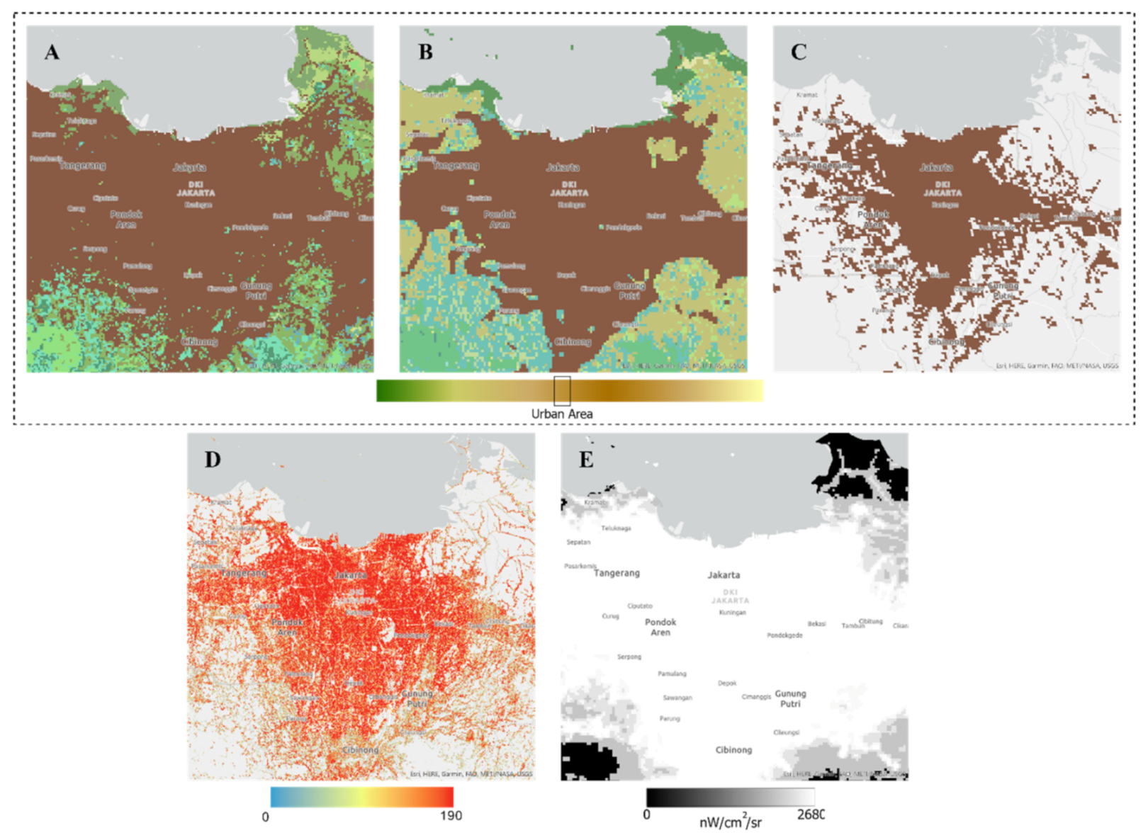
2.1.2. Remote Sensing-Based Land Use Land Cover Data

Land Use Land Cover (LULC) was used in extracting information on the Earth’s surface. Information related to land cover types and land use is needed considering the impact of land cover type information on the generation of estimated plastic waste. In this study, a LULC ESA CCI-LC product was selected [35], with a pixel resolution of 300 m. This LULC product was developed sustainably and processed with different input data, including AVHRR HRPT (1992–1999), SPOT-Vegetation (1999–2012), and PROBA-V (2013–2015). There are 37 land cover and land use classes in this product, including urban land cover types used as data input in this study. The urban land cover represents areas with high populations where common unmanaged plastic waste occurs on land. Additionally, the multi-products of LULC data from MODIS [36] and GLCNMO [37] were driven to support urban area sensitivity.

2.1.3. VIIRS Stray Light Corrected Night-Time Data

In this study, the night light data indirectly represented economic parameters. Night light data, specifically the Visible Infrared Imaging Radiometer Suite (VIIRS), were developed by the National Oceanic and Atmospheric Administration (NOAA) [38] with a product unit nW/cm2/sr. We, specifically, adopted VIIRS Stray Light Corrected Night-time data [43], an alternative configuration of the VIIRS Day-Night Band (DNB), to correct distorted light. The collected remote-sensing-based night-time data, however, is limited by the inability to extract high-quality data coverage due to cloud cover in certain regions, especially in tropical regions, such as Indonesia. Nevertheless, several studies have successfully reported that night light data can determine the distribution of access to electricity as a realisation of energy supply [44]. Several studies also show a positive correlation between night light levels and economic factors, such as GDP and other economic parameters [45,46]. Data analysis was performed in this study over one year in 2019, which then took the maximum data in each pixel using Google Earth Engine cloud-based data processing [47]. This analysis was performed to obtain the value with the maximum vulnerability location of the electrification distribution and the economy that will affect population density.

2.1.4. National Waste Management Information System (SIPSN)

Waste statistical data were obtained from the National Waste Management Information System (SIPSN) website, which was developed by the Ministry of Environment and Forestry of the Republic of Indonesia [26]. SIPSN is an online database platform created in 2017 following the Law of the Republic of Indonesia No. 18 of 2008, article 7b, and Government Regulation of the Republic of Indonesia No. 81 of 2012, article 34. SIPSN data were developed by the Indonesian Ministry of Environment and Forestry, adopting the basis of tabulation processing managed by local governments. Each City/Regency government inputs all waste data in Indonesia into one integrated dataset. The most recent published data are for 2017–2018, with the smallest administrative area in regencies/cities in this database. In this study, data on the percentage of plastic waste composition per regency/city in 2017–2018 was obtained. However, waste data from all regencies/cities were not available; therefore, several other approaches were adopted to complement the data.

2.1.5. River Streamflow Network and Estuary Data

To establish the detection of river estuaries connected to the sea, two sets of data are utilised. The first consists of river flow data compiled by Global Surface Water [40], which contains the temporal distribution of surface water from 1984 to 2018, while the second dataset includes statistical data on the area and changes in the water surface. The data were generated from 3,865,618 images of Landsat 5, 7, and 8, which were captured between 16 March 1984, and 31 December 2018. Each pixel image was grouped into either a water or non-water category, and the results were grouped into two time periods (1984–1999, 2000–2018) for visualising change detection. The rivers from the 2000–2018 epochs have been separated from other water cover classes. The second dataset is the coastline data collected by Natural Earth Data [41], which covers Earth’s entire coastline. The shoreline dataset product generated by Natural Earth is classified into three categories based on quality: great detail, medium detail, and low detail classes. In this study, the estuary is defined as a confluence between a river flow, which has been developed through Global Surface Water products, and a coastline, which has been developed by Natural Earth Data [41].

2.1.6. Data for Comparison Study

The absence of field data representing actual data related to plastic waste heaps is a limitation to determining the plastic waste distribution. To overcome this issue, study comparisons were conducted as there are several studies with the same objectives, which can be a basis for the comparison of available estimated results from other studies. Specifically, there are two studies related to the potential for plastic waste in the estuary, performed by Lebreton et al. [5] on the Indonesian territory in the global scale model and by Cordova et al. [32] in the Jakarta Bay area. Comparison of the values between different estuary points can be accomplished, especially on the data developed by Lebreton et al. [5], given that this study provides estuary waste data that can be accessed and processed using geographic information system (GIS) tools. The second approach compared the comprehensive study results for the amount of plastic waste in the estuary in Jakarta Bay calculated with the field data reported by Cordova et al. [32]. In addition to comparing point-to-point products from plastic estuary waste, data from the FLO1K annual model product of river flow changes were used [42]. The FLO1K consisted of the average, maximum, and minimum streamflow values for each year from 1960–2015. This streamflow product was developed using artificial neural network (ANN) regression, which was integrated into monthly observation measurements at 6600 observation stations worldwide. The FLO1K supporting data were used to show a relationship between streamflow slowdown and the index product of plastic waste disposal potential.

2.2. Methodology

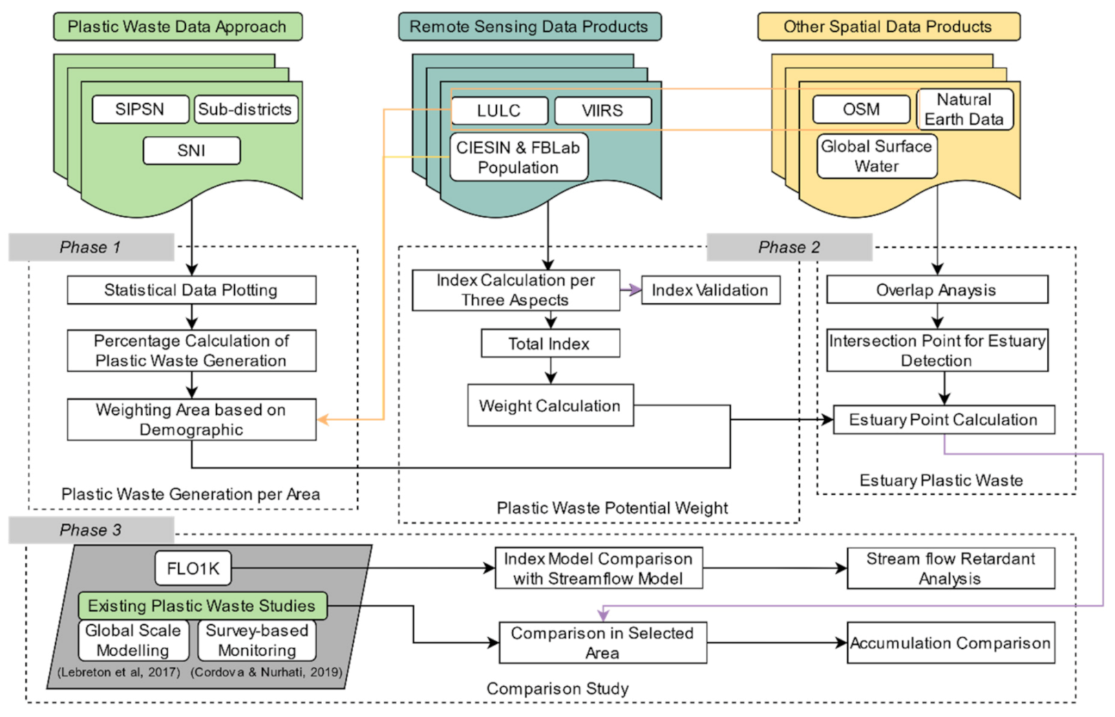
2.2.1. General Methodology

The data processing in this study was divided into three main phases. The first included the generation of plastic data per administrative unit using SIPSN and SNI data. The second phase included the development of an index for plastic waste disposal potential, resulting from the integration of LULC, population density, and night-time light data. Combining the statistical data of plastic per administrative unit and the waste potential index resulted in the distribution of land plastic waste disposal per unit pixel. Development of the estuary point was then accomplished through an overlay process of the coastline data with the river flow data. The final phase included the estimation of estuary plastic waste by calculating the accumulated value of plastic waste disposal, facilitating the calculation of the estuary’s total waste. Three scenarios of mismanaged plastic waste generated in each area were developed based on historical data and engineering judgements. The general structure of the work phases for this study is presented in Figure 1, while Figure 2 presents the parameters for plastic waste disposal indices.

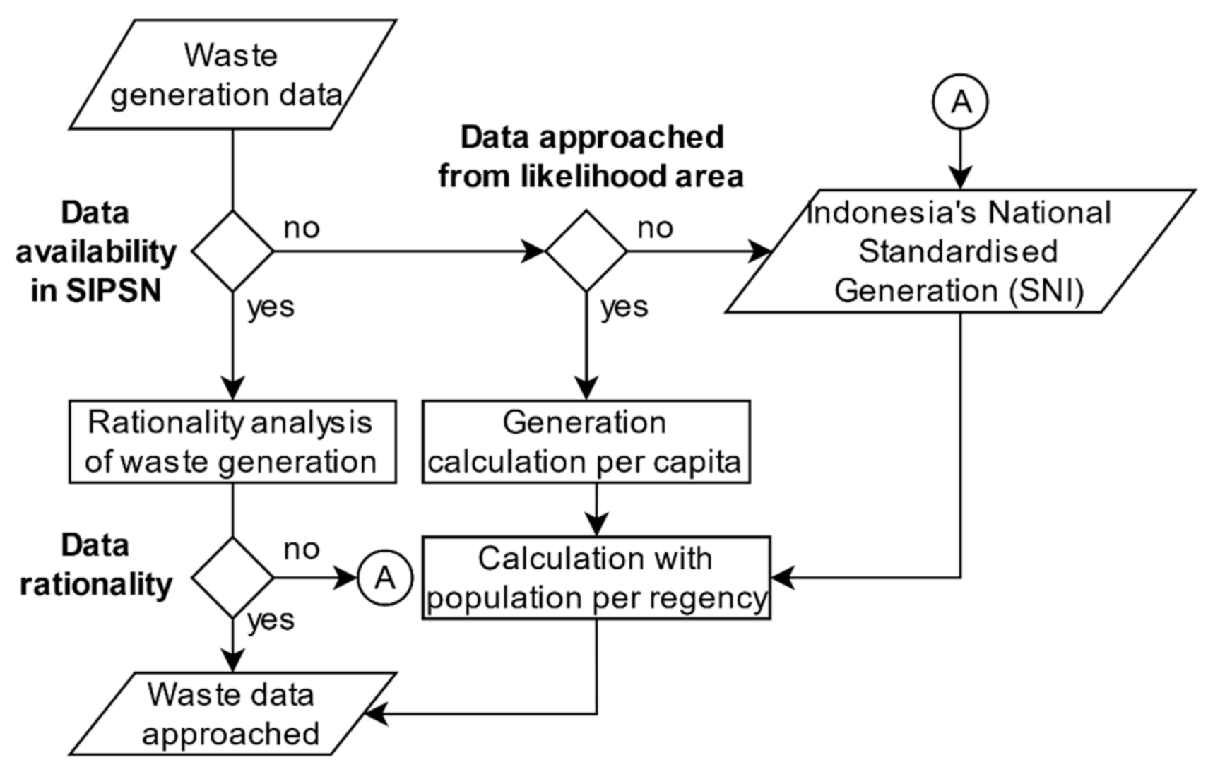
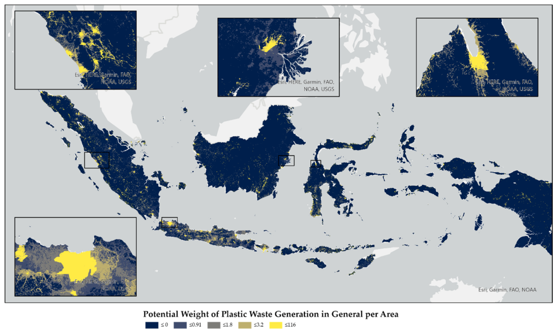
2.2.2. Estimating Plastic Waste Generation per Administrative Unit

Establishing total plastic per administrative unit is the first phase in estimating the amount of plastic waste in river estuaries. For this phase, the composition data were extracted using three approaches. In the first approach, the SIPSN dataset served as a reference for the primary data source [26]. The second approach will be conducted if data were not available, then the amount of plastic per capita for the region was assumed to be identical to another location with a similar population density, population size, and area. For the third approach, if the comparison of characteristics did not match, the amount of plastic per capita was obtained from the national standard: SNI 10-3983-1995 regarding the Specifications for Solid Waste Generation for Medium and Small Cities [48]. The data for the generation of plastic waste had a value per pixel; that is, there was one value per 300 m2. The flowchart for establishing the amount of total plastic at the source is presented in Figure 3.
The waste generation per capita data (weight/person/day) was used to multiply the population data to obtain the total waste generation in one city/regency in the day’s unit. Population data were obtained by integrating the population data from the Central Bureau of Statistics for the year 2018 [49]. The plastic waste composition figure was obtained from SIPSN documentation and several other approaches (area characterisation and Indonesia’s national standard of waste generation); therefore, the plastic waste generation figure can be calculated using Equation (1).
P W q t y = W G c a p × p o p u l a t i o n × % P W
where PWqty is the value of a quantity of plastic waste (kg/day), while WGcap represents waste generation per capita (kg/person/day), and %PW is the percentage of plastic waste (%). After tabulating the data for the amount of plastic in tonnes per day in each regency, the data were combined with spatial data for regency administrative areas obtained from the Geospatial Information Agency [39]. The data were then converted into a pixel base in a raster format with a pixel size of 300 × 300 m to obtain data per regency in the raster.
Through the integration and application of SIPSN data [26], data linkage assumptions, and SNI, spatial data on the value of waste generation was established per regency area. The smallest administrative units that could be processed based on data input in this study were regency and city administrative units. The plastic waste generation unit was in weight (tonnes/day), with an initial indication that one regency had the same average value. This method also part of the developing study for waste generation data approach [50] for modelling of plastic waste generation per possible smallest administrative unit.

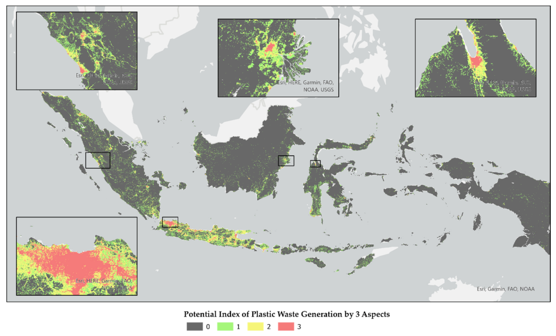
2.2.3. Developing Potential Index of Plastic Waste Disposal

It has been discussed previously that plastic waste generation was analysed from three different aspects: environmental, social, and economic. For the development of the index, which carried the weight of the potential for plastic waste generation disposal, the data reviewed were related to residential areas and areas occupied by humans considered as the main factor causing waste generation [23]. There were three datasets used: land cover data, population density, and night-time light data. Land-use cover data were used to identify residential areas obtained in the urban areas. The identification of land-use cover only focused on urban areas; therefore, steps exercised in data preparation were only for forming data classifications where residential areas were worth class 1, while non-residential areas were worth class 0.
Social aspects were reviewed based on population distribution, which was then used as population density. The OSM building data with the basic polygon shape was converted into points by identifying the centroid points on the polygons, which were processed to produce household density products. The points that possessed values were calculated by the number per coverage using the density principle of the points by calculating and analysing spatially based on a particular area (300 m pixel area) along with the integration of the population density within 30 m. The building density data were classified into classification by referring to SNI 03-1733-2004 related to the housing environment’s planning procedures in urban areas [51]. The four classes of area classifications based on density are presented in Table 2. The index was valued as class 1 when the population density reached a very dense class due to the density value with potential for waste generation.
The economic aspect applies the indirect parameter in the form of night-time light data from the VIIRS product, which provides data on average night-time light per month, where the data update has been recently performed; however, the data used were from 2019. The economic aspect was represented by night-time light, assuming that it was fully correlated with economic data in the area as the indicator of intense human activity. Night-time light data were classified by the geometrical interval classification method, which is suitable for classifying economic activity [52]. The geometrical interval method can be simply stated as a method that combines other classification methods such as natural breaks, quantiles, and equal intervals. This method focuses on class division using the power quantification principle with data that can be ideally distributed. Classes were established at intervals that focused on each class; therefore, the class of night-time data was assessed to qualitatively assess the low, medium, and high classes. The three aspects were calculated; hence the index was obtained every 300 m between classes 0 and 3 by representing every potential aspect obtained. The weight was obtained by calculating the tabulation with pixel basis operations, with each regency having a total weight of 1. To accomplish this, it was necessary to identify the index per regency using each regency’s unique code with a total of 415 regencies in Indonesia. The weight calculation was performed according to Equation (2):
W = I Σ I × 100 %
where W is the weight to be defined in percentage, I is the formed index value, and ΣI represents the total index in one regency.

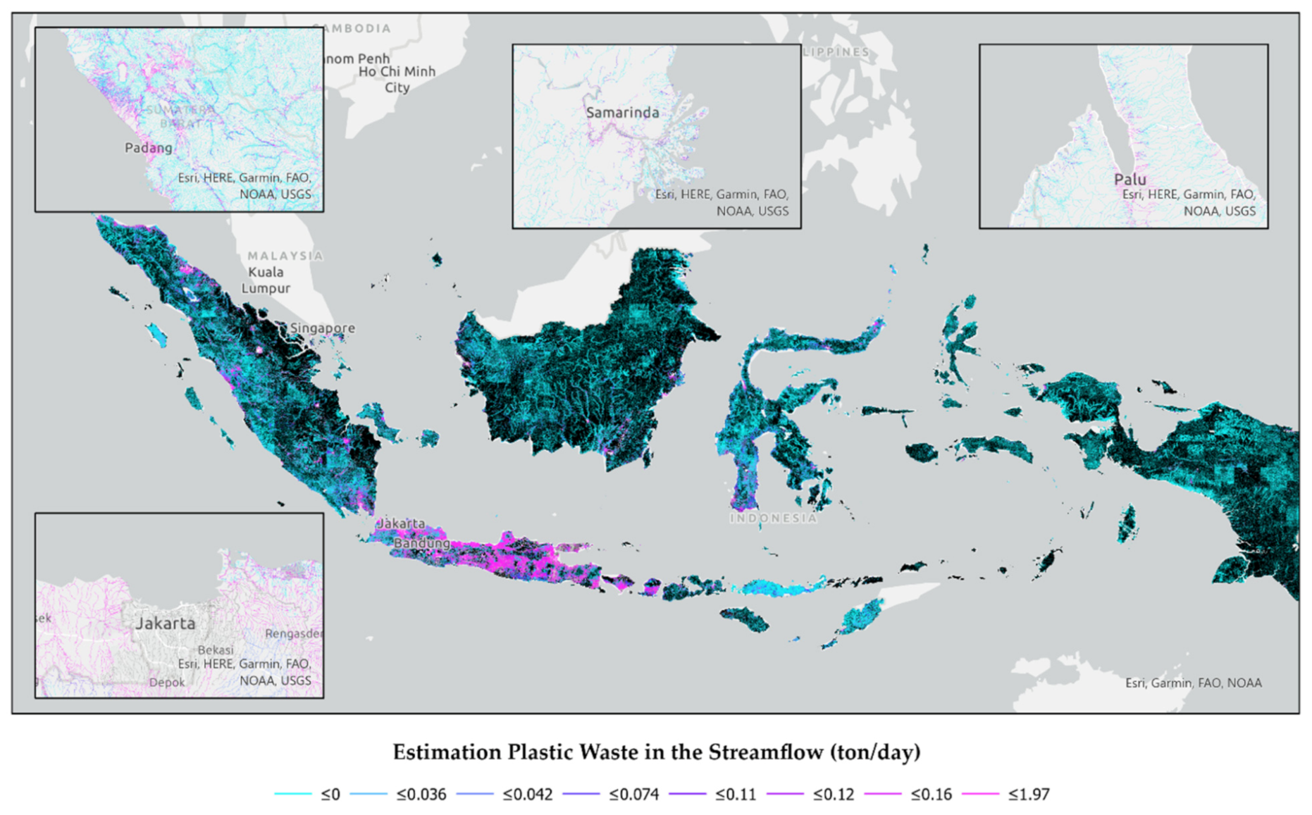
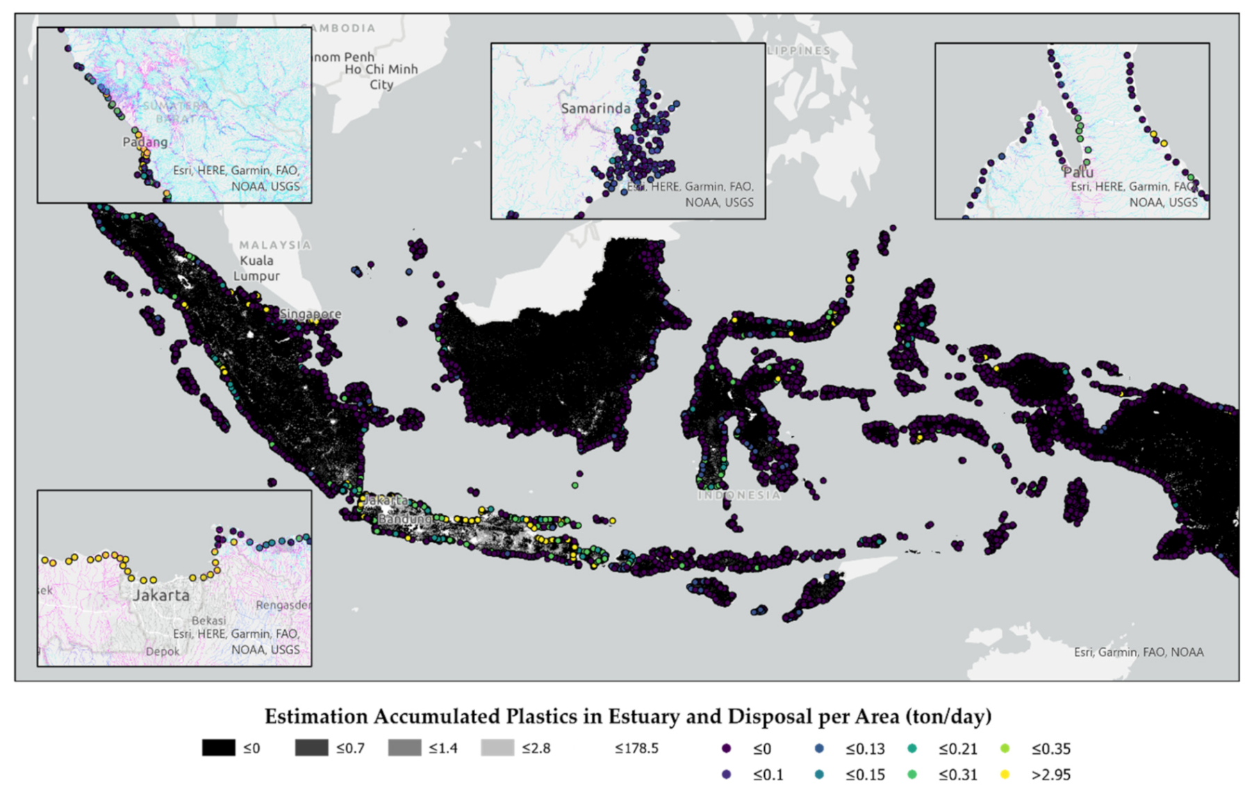
2.2.4. Modelling Marine Debris of Plastic for the Coastal Area

The final phase comprised the identification of plastic waste generation at each estuary. Estuaries were identified from overlapping locations that are a confluence of rivers and seas. To determine the locations, a spatial analysis of GIS was used with the overlay analysis method, which is a methodology used to determine the optimal location or suitability analysis. One of the advantages of this technique is that it can be applied to data with both the same and multiple data scales to produce integrated data. Referring to the two results obtained from the two previous phases, specifically data on the plastic waste approach per pixel per regency and data on potential weight per regency, calculations were performed for the amount of assumed waste per pixel. The calculations were performed using Equation (3):
P l a s t i c   T o t a l = W × Σ P
where W is the weight value used, and ΣP is the amount of plastic (tonnes/day), where both are processed with the coverage area per regency/city.
In identifying plastic waste in the river area, an overlay method was re-conducted between the amount of plastic waste per pixel and the river data. The features obtained for estuary identification were point features, and 8688 estuary points were produced for the Indonesian region. The outputs in the first and second phases were used as the input in the estuary flow analysis section. The result of load on the estuary was established by analysing the total overlay value of the waste in the pixels that the river passes through, which was then accumulated at the river end boundary, that is, the estuary; this conveys the general assumption that waste in an area of 300 × 300 m that passes through the river will potentially be unmanaged and wasted through the river flow.

3. Results

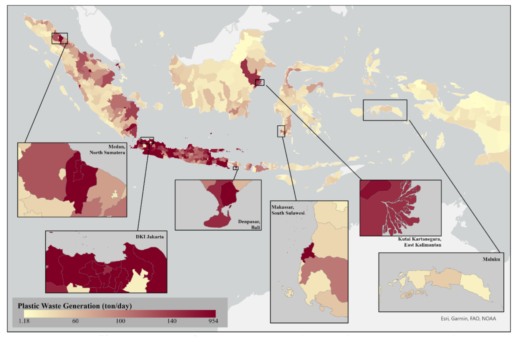
3.1. Plastic Waste Generation per Administrative Unit Estimation

Through the integration and application of SIPSN data, data linkage assumptions, and SNI, spatial data on the value of waste generation per administrative unit were obtained. The visualisation of the generation of plastic waste at the source was expressed in a colour range. Red indicated larger plastic waste generation, and blue indicated lower generation of plastic waste. The map of plastic waste generation data per regency can be observed in Figure 4, which also developed from the previous study to creating an approaching model of plastic waste generation data [50].
The results show that the total amount of plastic waste per regency was between 1.18 to 954 tonnes/day for one administrative regency and city area in Indonesian territory; this indicates that every regency and city in Indonesia has plastic waste generation that varies depending on the profile in the area. Some areas were grouped based on the demographic, which refers to population density, such as (a) DKI Jakarta represents high density, (b) Medan, North Sumatera represents reasonably high density, (c) Makassar, South Sulawesi represents reasonably low density, and (d) Merauke, Papua represents low density. Moreover, multiple variables were found to affect the amount of plastic waste generated in a regency. Additionally, it can be observed that plastic waste generation does not always directly relate to the population density level, as was observed for two examples in Java Island. Tasikmalaya Regency has a high population of 1,035,411 people (2018) with a plastic waste generation of 420.92 tonnes/day, compared to Bekasi City with a population of 3,003,920 people (2018) and plastic waste generation of 410.45 tonnes/day; this was due to the influence of high economic activity in the area, which resulted in the high demand for plastic.
The calculation of total waste generation in regencies and cities showed that Bogor Regency is the city with the most plastic waste generation, with a production value of 954.46 tonnes/day. Tangerang Regency and Bandung City then had plastic waste generation values of 617.85 tonnes/day and 604.05 tonnes/day, respectively. Some areas with small plastic waste generation include Seribu Island Administrative City, Supriori, and Selayar.

3.2. Potential Index of Plastic Waste Disposal

The plastic waste potential index is an index that describes the vulnerability of an area in its contribution to the disposal of plastic waste on land. The index was created based on three parameters: land use cover, population density, and night-time light. Each parameter contributes to a weight of 1, with a maximum index weight value of 3 and a minimum of 0 (Figure 5). By observing the results in Figure 5, it can be concluded that the potential index describes areas in the large-city categories (for example, DKI Jakarta and Makassar City areas). The large-city areas were characterised by variations from index classification around them, where a maximum potential index can also be identified, which reaches number 3. Figure 5 shows that the size of the index is directly proportional to the high economic activity level and high population density in urban areas.
Quantitatively, Indonesia has an index value of 0 in 94.54% of the area. An index of 0 indicates that it is not an urban area and has a low population and economic level. The index values 1, 2, and 3 covered 4.72%, 0.65%, and 0.08%, respectively, out of a total of 19,550,694.00 pixels that were processed in this research. The plastic waste potential index results were combined with plastic waste generation data per regency to indicate the potential weight of plastic waste in units of pixels covering one regency (see Figure 6).
The weight of the potential waste generation was distributed locally by means of each regency weighting, with the aim of potential weight was to examine the distribution value of waste generation in each region. The results of the potential weight were directly proportional to the results of the plastic waste potential index. However, a review is still needed for each regency. The percentage value of weight confirms how much potential for plastic waste disposal is in a regency of 300 × 300 m; this means that a coverage area of 9 Ha is the most possible in defining the smallest area of a regency.

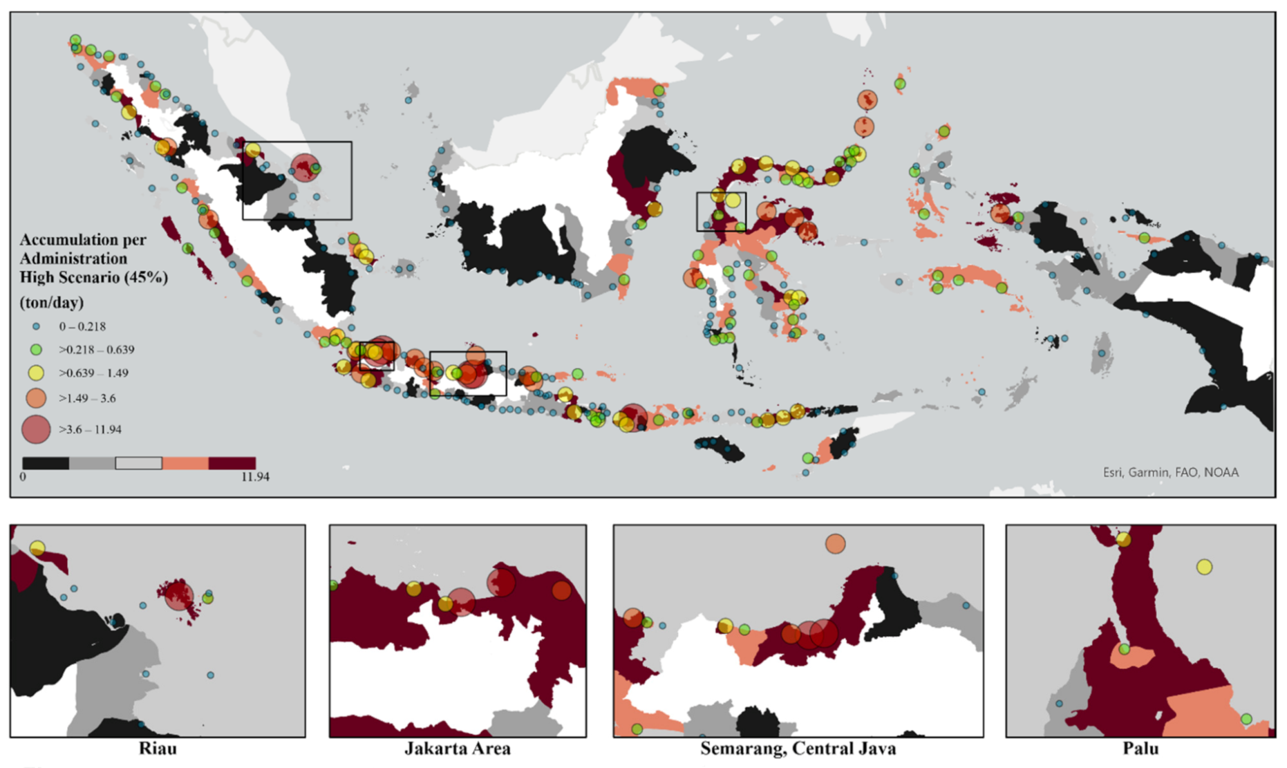
3.3. Plastic Waste Weight per Estuary Location

By acknowledging each pixel’s weight in the regency coverage and the amount of plastic produced in each regency, the distribution of plastic load per pixel is presented in Figure 7 in river flow and Figure 8 as the accumulation in the estuary. The distribution of land plastic waste generation per regency is considered the weight of potential local areas. Areas with higher weights disposed of greater amounts of plastic.
However, the distribution results are projective, assuming that the gap between areas with absolute potential and non-potential is highly incomparable. A projection of plastic waste disposal in the river area was developed from the resulting distribution to the estuary points before entering the waters. The assumption made is the worst-case scenario projection, where all plastic waste in an area enters the river system. Brighter colours in Figure 6 indicate a higher potential for dumping plastic waste. The intersection of coastline and river flow layer generated estuary points that have a tolerance of 300 m. The predicted load of plastic waste at the estuaries reached 5 tonnes/day at its highest, which resulted from the assumption that all plastic waste entered the ocean; thus, if this is calculated for all rivers (Figure 7), a high load of plastic waste is predicted (Figure 8).
The weights were used to establish the waste distribution result in smaller areas having a plastic load value. For each river, a scenario of 9 Ha through which the river had the same plastic load (assuming the river flow was homogeneous) resulted in total plastic waste per river in tonnes/day in Figure 8 in the full scenario (100%).

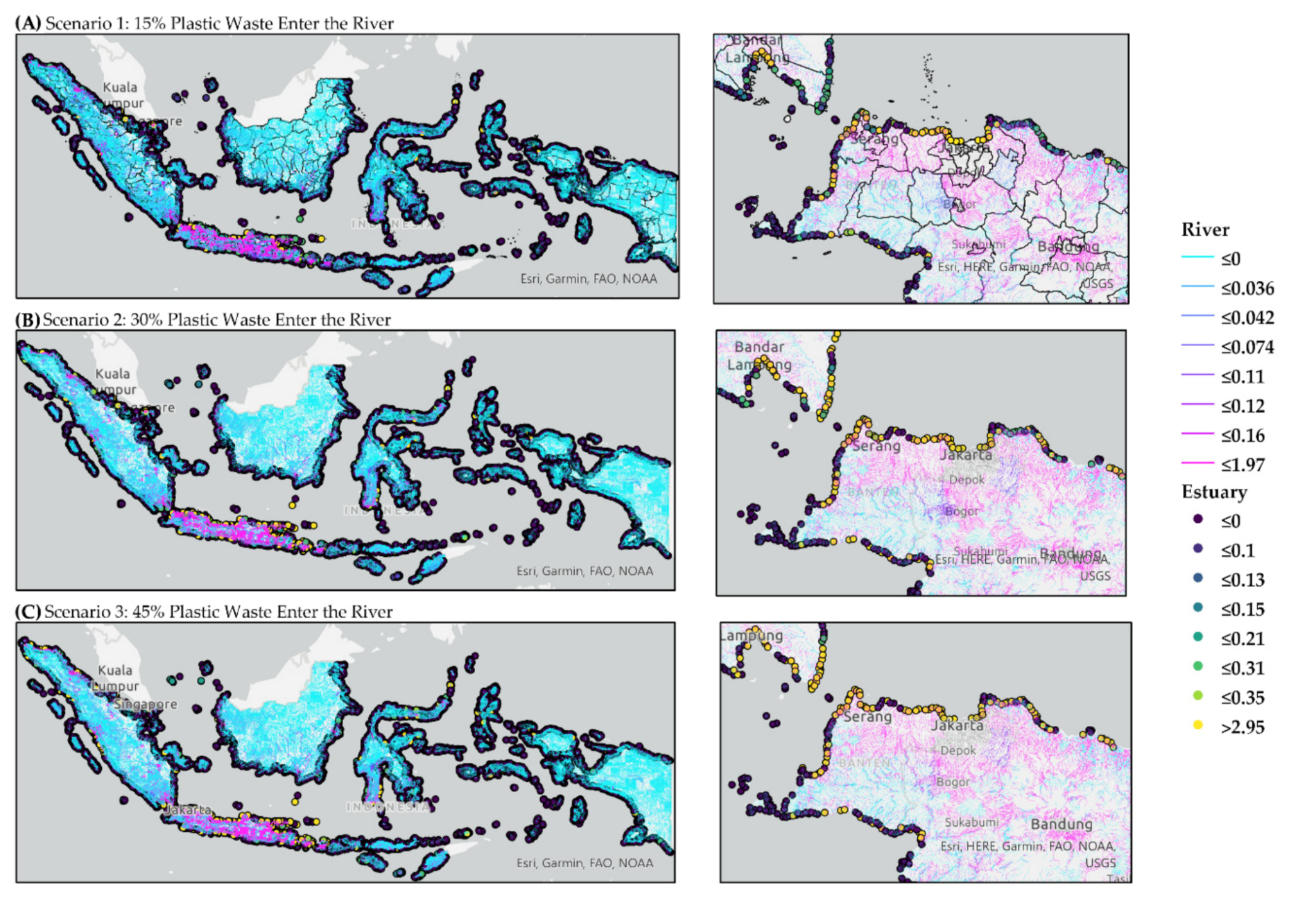
3.4. Scenarios of Plastic Waste Generation

To provide a model for the realisation of plastic waste disposal, a review of several reports was performed related to the measurement of the amount of marine debris integrated with the land area. Shuker obtained an average yield of plastic waste entering rivers in Indonesia’s territory as approximately 20% of the total land plastic [53]. Meanwhile, a local report, the Marine Debris Hotspot Rapid Assessment report in 2018, stated that, on average, Indonesia contributes 30% of land plastics, with a range of 15–20% plastic waste that escaped to nature, and 10–15% of plastic waste that was not well managed [53]. The report on Plastic Waste Poisons Indonesia’s Food Chain in 2019 explained that the value of plastic waste entering the ocean reaches 20–38% of the total plastic waste [24]. Following historical data and engineering judgements, the values of 15%, 30%, and 45% of unmanaged plastic waste that could potentially be dumped into rivers were exerted. In this case, the scenario development is also intended to determine if the percentage of mismanaged plastic waste is suitable to the actual conditions rather than only historical data or research. Projection development for three scenarios is presented in Figure 9.
From the results of the three scenarios, the volume of the plastic waste reaching the estuary can be seen to vary depending on the scenario. In the 15% scenario, the average amount of plastic waste transported to river estuaries in the Jakarta area was 7.45–11.6 kg/day. Using river estuary data and regency/city administrative area data, a statistical analysis was performed to evaluate the accumulation of plastic waste entering the river estuary from each regency/city. One endpoint in each regency/city was created to represent the river estuary’s location adjacent to these points (Figure 10). The average total plastic waste transported to river estuaries throughout Indonesia reached up to 2 tonnes/day based on statistical calculations. Figure 10 defines the worst-case scenario for plastic waste accumulation in one regency/administrative city where 45% of the plastic waste was discharged into the marine environment.
The statistical results of the plastic waste accumulation from each regency/city can be seen in Table 3, with a maximum value of 11.94 tonnes of waste in the Bekasi Regency. The statistical approach per regency/city can be applied for planning plastic waste management strategies. Based on the region, it can be observed that the DKI Jakarta area was not the largest contributor; therefore, other factors were also considered. An overview of the Central Sulawesi region (especially in the cities of Palu and Donggala) showed that this region had a high value compared to the nation’s capital, creating aftereffects in the natural disasters that hit the region, such as the Palu tsunami in September 2018 and the fact that the SIPSN approach data were for the 2017–2018 period. Additionally, it was assumed that the Bali region increased in local cultural activities, such as dumping offerings into the sea during specific event periods.

4. Discussion

The calculation of a load of plastic waste entering the ocean was estimated based on all plastic assumed to have a probability of flowing from the river to the estuary. The total amount of the unmanaged plastic load was assumed to be based on the approach value from the field data presented by SIPSN, the assumption of data per regency with its weight, as well as the assumption of waste generation in the generalisation of the classification of medium and small cities, according to applicable standards. The yield value per regency was calculated using results from the weight calculation to understand the distribution value. The weights were calculated per regency by considering the index obtained based on three aspects: land-use cover, population density, and night-time light economic activity in each region.

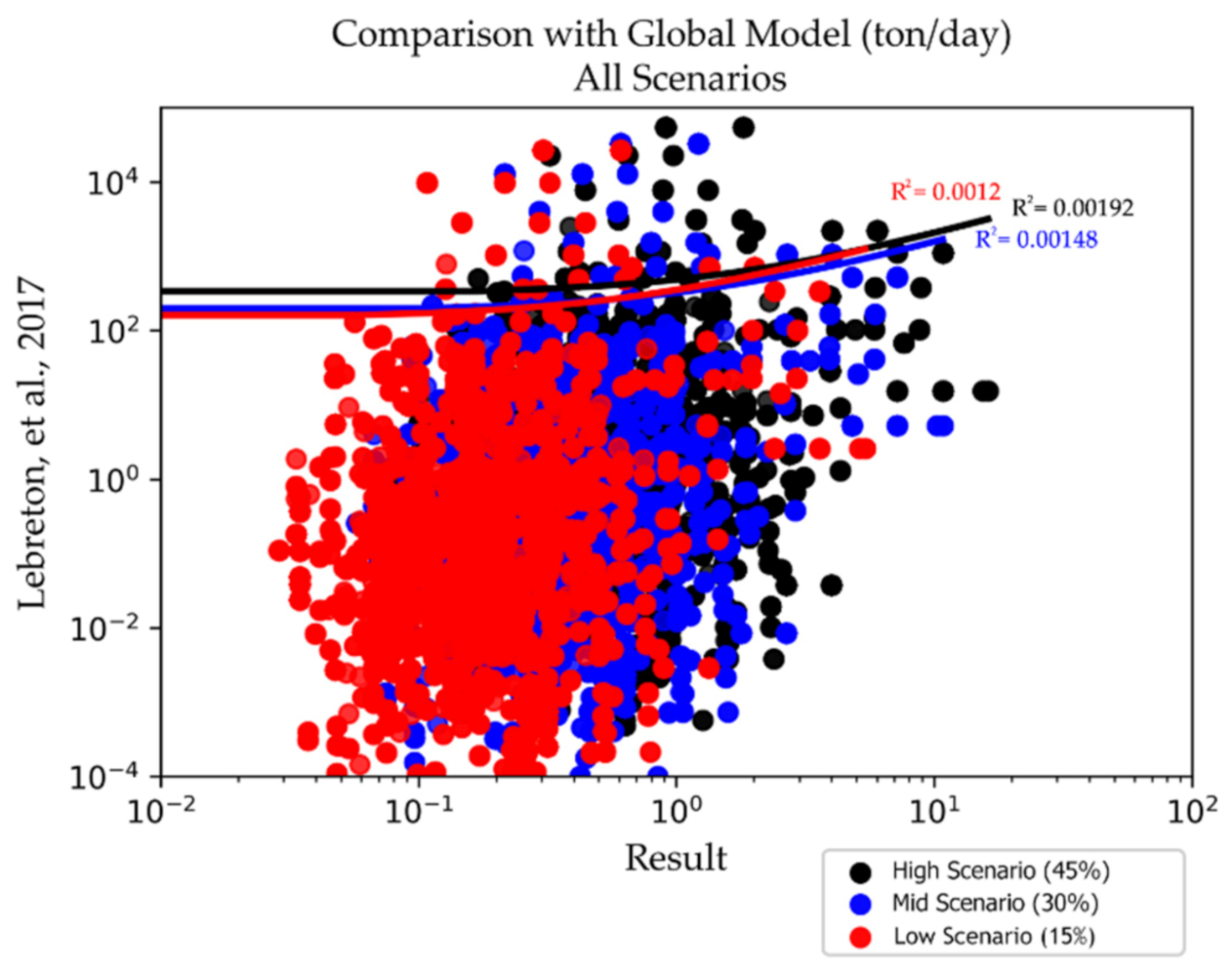
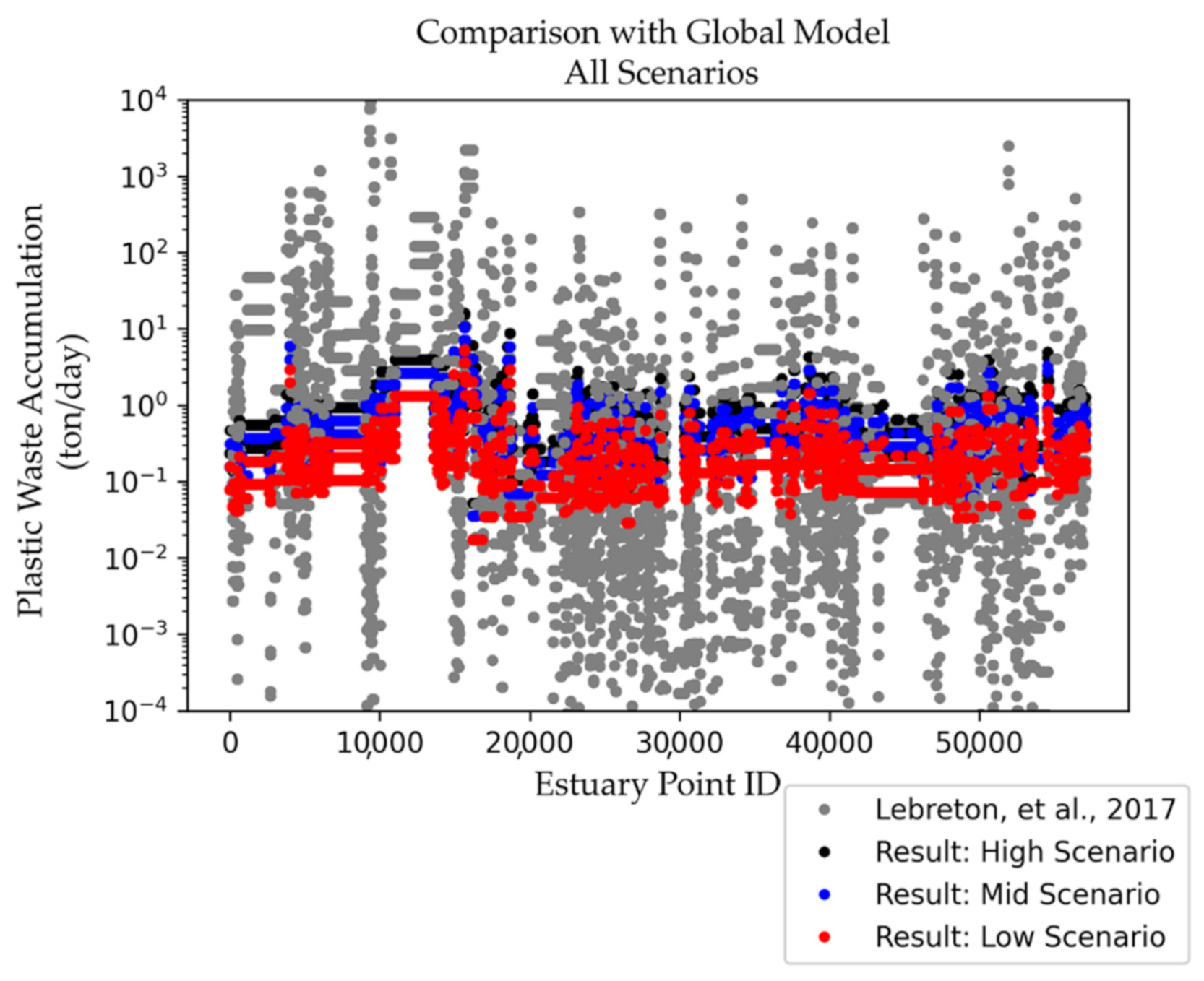
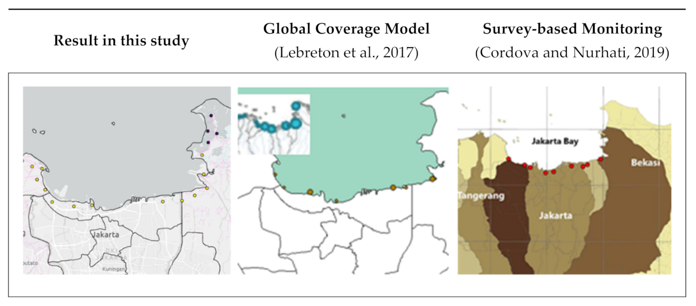
4.1. Comparison of Model and Data Existing of Plastic Waste Inputs from River

The final result of the three phases was a plastic load map per estuary. Comparisons were made with the research results on global models of plastics entering the oceans from rivers based on waste management, population density, and hydrological information by Lebreton et al. [5], which resulted in 739 similar points for comparison.
From the graphs in Figure 11 and Figure 12, it can be seen that the data from the research results of Lebreton et al. have higher and more varied yields. The differences resulted where data processing by Lebreton et al. using hydrological data parameters allowed the calculation of run-off flow, which is not discussed in this study. The research conducted by Lebreton et al. refers to the development of three scenarios: high, medium, and low, concerning seasonal patterns each month, in contrast to the development administered in research based on the estimated total percentage of daily plastics. Data comparison was reviewed at the point with a linear regression line revealing a large amount of data that did not exhibit direct linear comparisons between the research results and existing modelling. The differences in parameters and approaches represent factors in the estimation of plastic waste values in the estuary.
To compile comparisons with local area data and also in context with the survey-based result, comparisons were made with previous research on plastic waste in Jakarta Bay in Figure 13 [32]. This comparison showed the existence of 8.23 ± 2.44 tonnes/day of plastic waste, while in a global scale model [5], plastic waste reached 17.61 tonnes/day at high input. The estuary calculation result in this study at Jakarta Bay in the high scenario reached 7.2 tonnes/day; in the medium scenario, it reached 4.8 tonnes/day; in the low scenario, it reached 2.4 tonnes/day. The comparison of the three data sets provided preliminary results of a 2.03-fold difference from the global model [5] and a 1.08-fold difference from the survey-based study results [32]. The similarity of the results may have been due to the terms used to define the estuary outlets themselves, while our study and survey-based modelling used river outlet, where global scale buffer through more than 1 km detection as it results to the higher estimation.

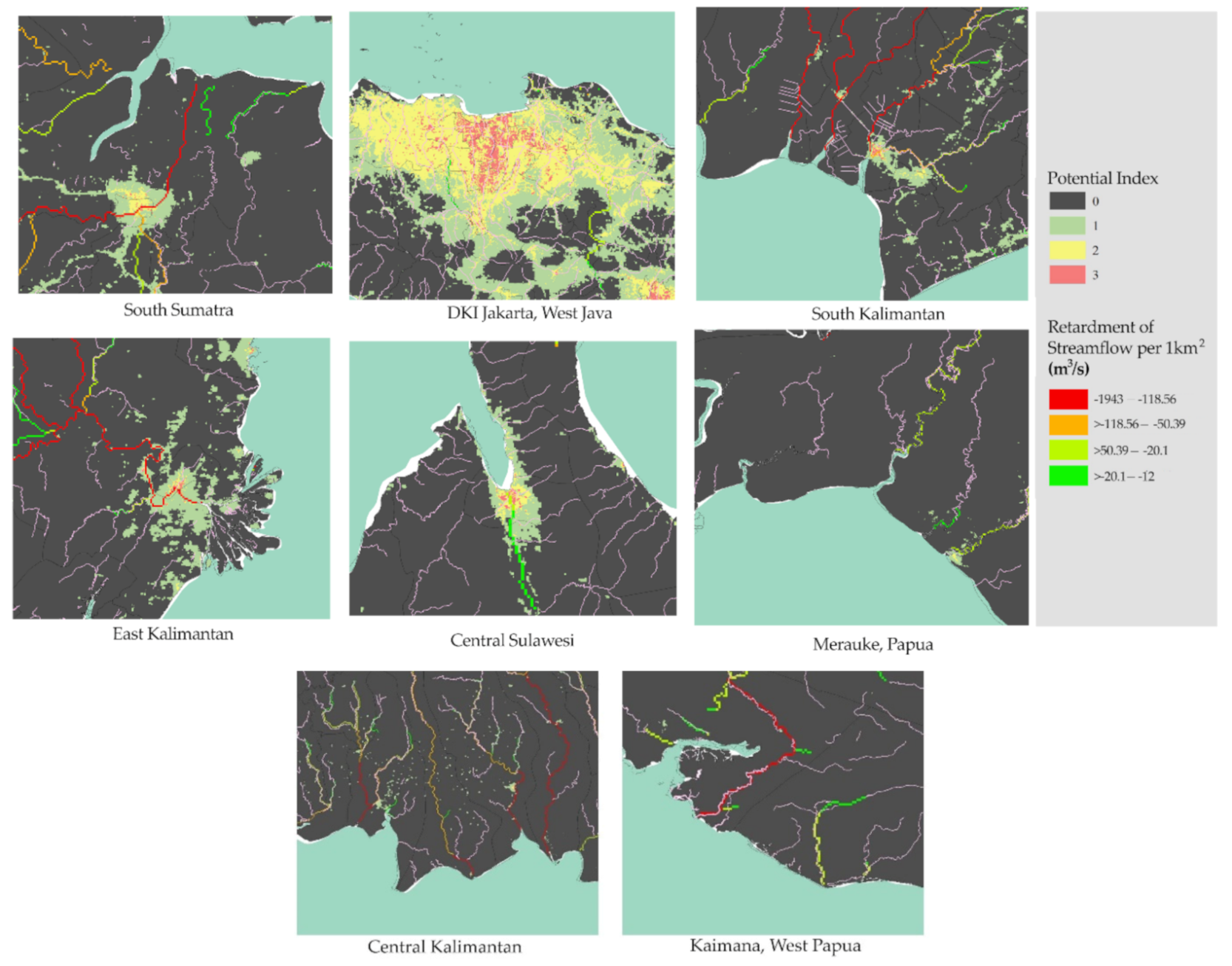
4.2. Impact of Plastic Waste on the Streamflow

The daily waste that flowed through the river estuary from 2000–2015 could potentially inhibit the river flow up to 1943 m3/s based on FLO1K modelling data products [42] (Figure 14), with the assumption that Indonesia’s mid-2007 per capita income (GDP) was +6.35%, where 2000 was a year of a steady increase in the eight years before, and 2015 in the eight years after the increase [54]. Data using a spatial resolution of 1 km presented potential areas in Palembang (South Sumatra), DKI Jakarta and West Java, Banjarmasin (South Kalimantan), Delta Mahakam (East Kalimantan), Palu (Central Sulawesi), and Merauke (Papua), thus demonstrating that, quantitatively, plastic waste has the potential to obstruct river flow. As for Indonesia’s full coverage, rivers directly connected to their estuary points had their flow slowed down to 21 m3/s. The slowing down of the river streams would yield other issues, such as flooding due to seasonal rainfall. Heavy rainfall would accelerate water current due to the addition of water masses in a short amount of time, thus causing the water to find another way to discharge the excess water mass in the river streams. In an ideal situation, water will flow in the river streams; however, the existence of plastic waste on river streams would demand alternative ways to discharge its masses, resulting in flooding to the urban area. A special review was performed for areas experiencing a slowdown in river flow with a low potential index in the Central Kalimantan region and Kaimana Regency in West Papua. The authors described an additional factor, other than waste entering the rivers, that serves to inhibit river flow rates, that is, soil sedimentation [55], which could have been caused by deforestation [56,57]. This is a concern since Central Kalimantan and Kaimana are mining areas, which represents a major cause of deforestation. The validation results with river flow data prove that the plastic’s potential supports the modelling of plastics accumulated from the land to the ocean until 2015, with 79% plastic waste in the coastal integration area [58].

4.3. Limitations

This study has several shortcomings, such as technical problems and assumptions used in the study. Some examples of technical problems, specifically the large grid resolution, represent bias factors in the simulation of plastic waste emptying into rivers. Additionally, there are limited data and previous studies on the material flow of plastic waste at Indonesia’s sub-regency level. Moreover, there is no data comparison between the model results and field data. The assumptions applied during classification for indexing could be developed by using the AHP classification method with expert-based judgement.

4.4. Further Research Prospects

As modelling of marine plastic requires an approach that incorporates strategic solutions within spatial analysis, further improvement of the proposed strategy is required to allow for its application in policy-making to set priority zones.

4.4.1. Improvisation with Hydrological and Basin Modelling

Waste accumulation in river estuaries can be calculated through a field-based approach, primarily involving watershed analysis (DAS). In the DAS approach, the first delineation of the watershed from each river mouth can be accomplished. Each cell of the raster map used/generated can be clipped to calculate the accumulation of waste that occurs downstream. In this physical unit-based analysis, the morphometry and watershed characteristics will determine the amount of waste that will accumulate downstream. This is achieved through a process analogous to determining the amount of sedimentation that occurs in a watershed compared to the total erosion that occurs since part of the transported eroded materials settle in the river before reaching downstream. The total portion of waste that ultimately reaches downstream can be similarly estimated since not all waste will be transported downstream, as some might remain stuck in the river bodies or transported and processed by humans.

4.4.2. Improvisation in Coastal Region Analysis

Due to the complexity of the coastal area, coastal region analysis has the capacity to improve the accumulation of marine debris in coastal areas. The coastal region differs based on environmental conditions. [59] Specifically, the primary coast is a coastal area that is formed by non-marine agents (i.e., land erosion, deposition, and volcanic coast), while the secondary coast is formed by marine processes (i.e., wave erosion, marine deposition, and coastal build by organisms). The different types of coastal regions exert different influences on marine debris. Moreover, coastal areas are also vulnerable to climate change. In fact, it was estimated that climate change would cause an approximate 40 cm increase in sea level within several regions in Asia by the end of the 21st century, 20% of which will occur in Southeast Asia, including Indonesia [60]. Therefore, coastal region analyses, as well as further analysis of the effects imposed by climate change in coastal regions within the Indonesia area, will improve the analysis of marine debris distribution and accumulation in coastal regions.

4.4.3. Application for Modelling the Movement of Waste in the Sea

The use of hydrodynamic model simulations can provide additional information on plastic waste movement patterns in the ocean that originate from river estuaries. Hydrodynamic model simulations can model the dynamics of the coast and the sea, which will affect the movement pattern of waste in the water area around or beyond the river estuary. With hydrodynamic model simulations, we can also observe whether plastic waste in the river estuary originates from the upstream river or is transported by ocean currents from other places. Additionally, we can predict which areas will be affected by plastic waste distribution in the sea. Using the baseline data approach is also proportionate to the importance of tracking marine plastic pollution to its dispersion in the ocean region included at a multi-national level. Therefore, modelling of the marine litter of plastic waste must also be implemented when the data regarding plastic waste generation is available at the regency or municipality level.

5. Conclusions

From this study, we present an estuarial solid waste model encompassing 8688 locations across Indonesia with a remote sensing-intensive approach. The model accounts for spatiotemporally varying environmental, social, population, and economic factors. Urban areas are delineated using land-use cover maps, economic patterns are determined based on night-time lightmaps, and solid waste generation is calculated using population density maps. The model estimates a total unmanaged solid waste generation of 289 tonnes/day nationwide to conclude the first generation of plastic waste in the estuary in one day. The methodology presented, however, requires further improvements as differences in the comparisons between the global scale and this survey remain. Some possible future directions are to incorporate a physical processes-based solid waste generation calculation unit, such as using watershed analysis (DAS). Instead of determining estuarial solid waste contribution based on whether a computation cell touches any river feature, parameterised hydrological processes inside an HRU should determine a cell’s contribution towards estuarial solid waste accretion. Another possible future direction is to incorporate machine learning methodologies to predict solid waste generation based on predictor variables, e.g., population density, night-time light, and land-use cover. The major drawback of a fine-tuned approach is that it relies heavily on human judgement, which could unintentionally introduce biases in the analysis. In contrast, machine learning approaches, such as profound learning, favour raw values, thus letting the model learn from its data. As an approach for tackling marine plastic pollution, this strategy can be applied during policy-making to establish priority zones for plastic waste management.

Author Contributions

Anjar Dimara Sakti and Aprilia Nidia Rinasti conceived and designed the experiments; Aprilia Nidia Rinasti and Anjar Dimara Sakti performed the experiments; Aprilia Nidia Rinasti, Anjar Dimara Sakti, Elprida Agustina, Hanif Diastomo, Zuzy Anna and Ketut Wikantika analysed the data; Aprilia Nidia Rinasti, Anjar Dimara Sakti and Elprida Agustina pre-processed the base datasets; Aprilia Nidia Rinasti, Anjar Dimara Sakti, Elprida Agustina, Hanif Diastomo, Fickrie Muhammad, Zuzy Anna and Ketut Wikantika wrote the paper; all authors read the paper and provided revision suggestions. All authors have read and agreed to the published version of the manuscript.

Funding

This project was funded in 2021 by the Capacity Building Research Program for ITB Young Scientists by the Institute of Research and Community Service, Institut Teknologi Bandung.

Institutional Review Board Statement

Not applicable.

Informed Consent Statement

Not applicable.

Data Availability Statement

The datasets generated during and/or analysed during the current study are available from the corresponding author on reasonable request.

Acknowledgments

The authors are grateful to acknowledge the support from the Institute of Research and Community Service, Institut Teknologi Bandung and United Nations Economic and Social Commission for Asia and the Pacific (UN-ESCAP). We also thank the anonymous reviewers whose valuable comments greatly helped us to prepare an improved and clearer version of this paper. All persons and institutes who kindly made their data available for this analysis are acknowledged.

Conflicts of Interest

The authors declare no conflict of interest.

References

  1. Connecticut Plastics. Perfect Plastic: How Plastic Improves Our Lives. Available online: http://www.pepctplastics.com/resources/connecticut-plastics-learning-center/perfect-plastic-how-plastic-improves-our-lives/ (accessed on 25 April 2020).
  2. Neumann, B.; Vafeidis, A.T.; Zimmermann, J.; Nicholls, R.J. Future Coastal Population Growth and Exposure to Sea-Level Rise and Coastal Flooding—A Global Assessment. PLoS ONE 2015, 10, e0118571. [Google Scholar] [CrossRef] [PubMed] [Green Version]
  3. Gall, S.C.; Thompson, R.C. The impact of debris on marine life. Mar. Pollut. Bull. 2015, 92, 170–179. [Google Scholar] [CrossRef] [PubMed]
  4. Thompson, R.C.; Olsen, Y.; Mitchell, R.P.; Davis, A.; Rowland, S.J.; John, A.W.G.; McGonigle, D.; Russell, A.E. Lost at sea: Where is all the plastic? Science 2004, 304, 838. [Google Scholar] [CrossRef] [PubMed]
  5. Lebreton, L.C.M.; van der Zwet, J.; Damsteeg, J.-W.; Slat, B.; Andrady, A.; Reisser, J. River plastic emissions to the world’s oceans. Nat. Commun. 2017, 8, 15611. Available online: https://figshare.com/articles/dataset/River_plastic_emissions_to_the_world_s_oceans/4725541 (accessed on 28 June 2021). [CrossRef] [PubMed]
  6. Lebreton, L.; Andrady, A. Future scenarios of global plastic waste generation and disposal. Palgrave Commun. 2019, 5, 6. [Google Scholar] [CrossRef] [Green Version]
  7. Brooks, A.L.; Wang, S.; Jambeck, J.R. The Chinese import ban and its impact on global plastic waste trade. Sci. Adv. 2018, 4, eaat0131. [Google Scholar] [CrossRef] [PubMed] [Green Version]
  8. Rochman, C.M.; Hoh, E.; Kurobe, T.; Teh, S.J. Ingested Plastic Transfers Hazardous Chemicals to Fish and Induces Hepatic Stress. Sci. Rep. 2013, 3, 3263. [Google Scholar] [CrossRef]
  9. Wilcox, C.; Mallos, N.J.; Leonard, G.H.; Rodriguez, A.; Denise Hardesty, B. Using expert elicitation to estimate the impacts of plastic pollution on marine wildlife. Mar. Policy 2015, 65, 107–114. [Google Scholar] [CrossRef]
  10. Gillsäter, B. Ocean Sector Profile. Available online: https://www.worldbank.org/en/results/2013/04/13/oceans-results-profile (accessed on 21 October 2020).
  11. Axelsson, C.; van Sebille, E. Prevention through policy: Urban macroplastic leakages to the marine environment during extreme rainfall events. Mar. Pollut. Bull. 2017, 124, 211–227. [Google Scholar] [CrossRef]
  12. Kubowicz, S.; Booth, A.M. Biodegradability of plastics: Challenges and misconceptions. Environ. Sci. Technol. 2017, 51, 12058–12060. [Google Scholar] [CrossRef] [PubMed]
  13. Gallo, F.; Fossi, C.; Weber, R.; Santillo, D.; Sousa, J.; Ingram, I.; Nadal, A.; Romano, D. Marine litter plastics and microplastics and their toxic chemicals components: The need for urgent preventive measures. Envivon. Sci. Eur. 2018, 30, 13. [Google Scholar] [CrossRef] [PubMed]
  14. Teuten, E.L.; Saquing, J.M.; Knappe, D.R.U.; Barlaz, M.A.; Jonsson, S.; Björn, A.; Rowland, S.J.; Thompson, R.C.; Galloway, T.S.; Yamashita, R.; et al. Transport and release of chemicals from plastics to the environment and to wildlife. Philos. Trans. R. Soc. B 2009, 364, 2027–2045. [Google Scholar] [CrossRef] [PubMed] [Green Version]
  15. Gregory, M.R. Environmental implications of plastic debris in marine settings: Entanglement, ingestion, smothering, hangers-on, hitch-hiking and alien invasions. Philos. Trans. R. Soc. B 2009, 364, 2013–2025. [Google Scholar] [CrossRef] [PubMed]
  16. Rochman, C.M.; Browne, M.A.; Underwood, A.J.; van Franeker, J.A.; Thompson, R.C. The ecological impacts of marine debris: Unraveling the demonstrated evidence from what is perceived. Ecology 2015, 97, 302–312. [Google Scholar] [CrossRef] [PubMed] [Green Version]
  17. Kwon, B.G.; Koizumi, K.; Chung, S.-Y.; Kodera, Y.; Kim, J.-O.; Saido, K. Global styrene oligomers monitoring as new chemical contamination from polystyrene plastic marine pollution. J. Hazard. Mater. 2015, 300, 359–367. [Google Scholar] [CrossRef] [PubMed]
  18. Zettler, E.R.; Mincer, T.J.; Amaral-Zettler, L.A. Life in the “Plastisphere”: Microbial communities on plastic marine debris. Environ. Sci. Technol. 2013, 47, 7137–7146. [Google Scholar] [CrossRef] [PubMed]
  19. Simeonova, A.; Chuturkova, R. Macroplastic distribution (Single-use plastics and some Fishing gear) from the northern to the southern Bulgarian Black Sea coast. Reg. Stud. Mar. Sci. 2020, 37, 101329. [Google Scholar] [CrossRef]
  20. Severini, M.D.F.; Villagran, D.M.; Buzzi, N.S.; Sartor, G.C. Microplastics in oysters (Crassostrea gigas) and water at the Bahía Blanca Estuary (Southwestern Atlantic): An emerging issue of global concern. Reg. Stud. Mar. Sci. 2019, 32, 100829. [Google Scholar] [CrossRef]
  21. Gago, J.; Portela, S.; Filgueiras, A.V.; Pauly Salinas, M.; Macías, D. Ingestion of plastic debris (macro and micro) by longnose lancetfish (Alepisaurus ferox) in the North Atlantic Ocean. Reg. Stud. Mar. Sci. 2020, 33, 100977. [Google Scholar] [CrossRef]
  22. Pravettoni, R. Plastic Waste Produced and Mismanaged. Available online: https://www.grida.no/resources/6931 (accessed on 19 April 2020).
  23. Jambeck, J.R.; Geyer, R.; Wilcox, C.; Siegler, T.R.; Perryman, M.; Andrady, A.; Narayan, R.; Law, K.L. Plastic waste inputs from land into the ocean. Science 2015, 347, 768–771. [Google Scholar] [CrossRef]
  24. Petrlik, J.; Ismawati, Y.; DiGangi, J.; Arisandi, P.; Bell, L.; Beeler, B. Plastic Waste Poisons Indonesia’s Food Chain: Indonesia Egg Report. November 2019, pp. 1–20. Available online: https://ipen.org/documents/plastic-waste-poisons-indonesia-food-chain (accessed on 28 June 2021).
  25. European Commissioner for Environment (ECC). Maritime Affairs and Fisheries; Report. Our Ocean; EU: Brussels, Belgium, 2016. [Google Scholar]
  26. Direktorat Pengelolaan Sampah; Direktorat Jenderal Pengelolaan Sampah; Limbah, dan B3 Kementrian Lingkungan Hidup dan Kehutanan. Sistem Informasi Pengelolaan Sampah Nasional; Kementerian Lingkungan Hidup dan Kehutanan: Jakarta, Indonesia, 2021.
  27. Kementerian Perencanaan Pembangunan Nasional Republik Indonesia; Badan Perencanaan Pembangunan Nasional. Sustainable Development Goals; Badan Perencanaan Pembangunan Nasional: Jakarta, Indonesia, 2017.
  28. United Nations. Sustainable Development Goals; UN: New York, NY, USA, 2018. [Google Scholar]
  29. Waste Atlas. Available online: http://www.atlas.d-waste.com/ (accessed on 10 May 2020).
  30. Cózar, A.; Echevarría, F.; González-Gordillo, J.I.; Irigoien, X.; Úbeda, B.; Hernández-León, S.; Palma, Á.T.; Navarro, S.; García-de-Lomas, J.; Ruiz, A.; et al. Plastic debris in the open ocean. Proc. Natl. Acad. Sci. USA 2014, 111, 10239–10244. [Google Scholar] [CrossRef] [Green Version]
  31. Moy, K.; Neilson, B.; Chung, A.; Meadows, A.; Castrence, M.; Ambagis, S.; Davidson, K. Mapping coastal marine debris using aerial imagery and spatial analysis. Mar. Pollut. Bull. 2018, 132, 52–59. [Google Scholar] [CrossRef]
  32. Cordova, M.R.; Nurhati, I.S. Major sources and monthly variations in the release of landderived marine debris from the Greater Jakarta area, Indonesia. Sci. Rep. 2019, 9, 18730. [Google Scholar] [CrossRef]
  33. Open Street Map. GEOFABRIK Downloads: Asia. Available online: http://download.geofabrik.de/asia.html (accessed on 24 March 2020).
  34. Facebook Connectivity Lab and Center for International Earth Science Information Network—CIESIN—Columbia University. High Resolution Settlement Layer (HRSL). Source Imagery for HRSL © 2021 DigitalGlobe. 2016. Available online: https://www.ciesin.columbia.edu/data/hrsl/ (accessed on 1 May 2020).
  35. ESA Climate Change Initiative. CCI-LC Products. Available online: https://www.esa-landcover-cci.org/?q=node/164 (accessed on 21 January 2020).
  36. MODIS. MODIS/Terra+Aqua Land Cover Type Yearly L3 Global 500m SIN Grid V006. Available online: https://catalog.data.gov/dataset/modis-terraaqua-land-cover-type-yearly-l3-global-500m-sin-grid-v006 (accessed on 1 May 2020).
  37. United Nations Office for Outer Space Affairs. Global Map-Global Land Cover (GLCNMO) (ISCGM). Available online: http://www.un-spider.org/links-and-resources/data-sources/global-map-global-land-cover-glcnmo-iscgm (accessed on 1 May 2020).
  38. National Oceanic and Atmospheric Administration. Earth Engine Catalog: VIIRS Nighttime Day/Night Band Composites Version 1. Available online: https://developers.google.com/earth-engine/datasets/catalog/NOAA_VIIRS_DNB_MONTHLY_V1_VCMCFG?hl=en (accessed on 9 February 2020).
  39. Badan Informasi Geospasial. Peta Rupabumi Indonesia. Available online: https://tanahair.indonesia.go.id/portal-web (accessed on 10 January 2020).
  40. Pekel, J.-F.; Cottam, A.; Gorelick, N.; Belward, A.S. High-resolution mapping of global surface water and its long-term changes. Nature 2016, 540, 418–422. [Google Scholar] [CrossRef]
  41. Natural Earth. Coastline. Available online: https://www.naturalearthdata.com/downloads/ (accessed on 22 January 2020).
  42. Barbarossa, V.; Huijbregts, M.A.J.; Beusen, A.H.W.; Beck, H.E.; King, H.; Schipper, A.M. FLO1K, global maps of mean, maximum, and minimum annual streamflow at 1km resolution from 1960 through 2015. Sci. Data 2017, 5, 180052. Available online: https://figshare.com/articles/dataset/FLO1K_-_Maximum_Annual_Flow_Time_Series_1960-2015/5688919 (accessed on 28 June 2021). [CrossRef] [PubMed]
  43. Mills, L.S.; Zimova, M.; Oyler, J.; Running, S.; Abatzoglou, J.T.; Lukacs, P.M. Camouflage mismatch in seasonal coat color due to decreased snow duration. Proc. Natl. Acad. Sci. USA 2013, 110, 11660–11661. [Google Scholar] [CrossRef] [PubMed] [Green Version]
  44. Beyer, R.C.M. South Asia Economic Focus, Fall 2017: Growth Out of The Blue; World Bank: Washington, DC, USA; pp. 1–22.
  45. Dai, Z.; Hu, Y.; Zhao, G. The Suitability of Different Nighttime Light Data for GDP Estimation at Different Spatial Scales and Regional Levels. Sustainability 2017, 9, 305. [Google Scholar] [CrossRef] [Green Version]
  46. Hu, Y.; Yao, J. Illuminating Economic Growth; 2019 International Monetary Fund Working Paper/19/77; International Monetary Fund: Washington, DC, USA, 2019; pp. 1–56. [Google Scholar]
  47. Gorelick, N.; Hancher, M.; Dixon, M.; Ilyushchenko, S.; Thau, D.; Moore, R. Google Earth Engine: Planetary-scale geospatial analysis for everyone. Remote Sens. Environ. 2017, 202, 18–27. [Google Scholar] [CrossRef]
  48. SNI 10-3983-1995. Spesifikasi Timbulan Sampah Kota Sedang dan Kota Kecil; Badan Standardisasi Nasional: Jakarta, Indonesia, 1995; Available online: https://pesta.bsn.go.id/produk/detail/4328-sni19-3983-1995 (accessed on 28 June 2021).
  49. Badan Pusat Statistik. Statistik Indonesia 2018. Available online: https://www.bps.go.id/ (accessed on 10 January 2020).
  50. Rinasti, A.N.; Sakti, A.D.; Agustina, E.; Wikantika, K. Developing data approaches for accumulation of plastic waste modelling using environment and socio-economic data product. IOP Conf. Ser. Earth Environ. Sci. 2020, 592, 012013. [Google Scholar] [CrossRef]
  51. SNI 03-1733-2004. Tata Cara Perencanaan Lingkungan Perumahan di Perkotaan; Badan Standardisasi Nasional: Jakarta, Indonesia, 2004. [Google Scholar]
  52. Olanrewaju, L.; Babatunde, N.O. Spatial Modelling of Economic Activity in Nigeria Using Gross Domestic Product of Economically Active Population. IOSR J. Humanit. Soc. Sci. (IOSR-JHSS) 2015, 20, 66–72. [Google Scholar]
  53. Shuker, I.G.; Cadman, C.A. Indonesia—Marine Debris Hotspot Rapid Assessment: Synthesis Report; Working Paper Report No. 126686; World Bank Group: Washington, DC, USA, 2018; Volume 1, pp. 1–46. [Google Scholar]
  54. World Bank. OECD National Accounts. GDP Growth (Annual %)—Indonesia. Available online: https://data.worldbank.org/indicator/NY.GDP.MKTP.KD.ZG?locations=ID (accessed on 19 May 2020).
  55. ICRAF; World Agroforestry Centre. Rewarding Farmers for Reducing Sedimentation, Indonesia [pdf]. Available online: https://oppla.eu/casestudy/17593 (accessed on 20 May 2020).
  56. Zeraatpishe, M.; Khaledian, Y.; Ebrahimi, S.; Sheikhpour, H.; Behtarinejad, B. The Effect of Deforestation on Soil Erosion, Sediment and Some Water Quality Indicates. In Proceedings of the 1st International Conference on Environmental Crisis and its Solutions, Kish Island, Iran, 13 February 2013; pp. 602–607. [Google Scholar]
  57. Restrepo, J.D.; Kettner, A.J.; Syvitski, J.P.M. Recent deforestation causes rapid increase in river sediment load in the Colombian Andes. Anthropocene 2015, 10, 13–28. [Google Scholar] [CrossRef]
  58. Lebreton, L.; Egger, M.; Slat, B. A global mass budget for positively buoyant macroplastic debris in the ocean. Sci. Rep. 2019, 9, 12922. [Google Scholar] [CrossRef] [Green Version]
  59. Shepard, F.P. Submarine Geology, 3rd ed.; Harper & Row: New York, NY, USA, 1973. [Google Scholar]
  60. Cruz, R.V.; Harasawa, H.; Lal, M.; Wu, S.; Anokhin, Y.; Punsalmaa, B.; Honda, Y.; Jafari, M.; Li, C.; Huu Ninh, N. Asia. Climate Change: Impacts, Adaptation and Vulnerability. Contribution of Working Group II to the Fourth Assessment Report of the Intergovernmental Panel on Climate Change; Parry, M.L., Canziani, O.F., Palutikof, J.P., van der Linden, P.J., Hanson, C.E., Eds.; Cambridge University Press: Cambridge, UK, 2007; pp. 469–506. [Google Scholar]
Figure 1. The overall framework of this study.
Ijgi 10 00481 g001
Figure 2. Remote sensing data product parameter in Jakarta Area: (A) LULC: ESA CCI-LC (B) LULC: GLCNMO (C) LULC: MODIS built-up, (D) population density: CIESIN-Facebook Connectivity Lab, and (E) Nightlight: VIIRS.
Ijgi 10 00481 g002
Figure 3. A flowchart of data source selection with area boundaries of the regency.
Ijgi 10 00481 g003
Figure 4. Plastic waste generation per regency area in Indonesia by tonne on a daily basis.
Ijgi 10 00481 g004
Figure 5. The potential index of plastic waste generation in Indonesia by three aspects.
Ijgi 10 00481 g005
Figure 6. The potential weight per area of plastic waste generation in general.
Ijgi 10 00481 g006
Figure 7. The flow of plastic waste from streamflow (tonne/day).
Ijgi 10 00481 g007
Figure 8. Accumulated plastic waste from streamflow through estuary.
Ijgi 10 00481 g008
Figure 9. Developing scenarios of plastic waste from streamflow through an estuary: (A) low case scenario in 15%; (B) moderate case scenario in 30%; (C) high case scenario in 45%.
Ijgi 10 00481 g009
Figure 10. Accumulation of plastic waste from streamflow trough estuary per coastal regency based on scenario 3.
Ijgi 10 00481 g010
Figure 11. A comparison of Lebreton et al. [5] input data (2017) and Indonesia’s overall estuaries by scatter plot.
Ijgi 10 00481 g011
Figure 12. A comparison of Lebreton et al. [5] input data (2017) and Indonesia’s overall estuaries by estuary point ID.
Ijgi 10 00481 g012
Figure 13. Result comparison of plastic debris accumulation research in the estuaries at Jakarta Bay.
Ijgi 10 00481 g013
Figure 14. A comparison between FLO1K [42] products of annual streamflow through the potential index.
Ijgi 10 00481 g014
Table 1. Data used in this research study.
NoDataProductPhaseSourceType of Data
1.Household PolygonGeofabrik.de 2020Plastic Waste Generation Index
on Land-based
[33]Raster—300 m
2.PopulationCIESIN and Facebook Connectivity Lab 2016[34]Raster—30 m
3.LULCESA CCI-LC 2015[35]Raster—300 m
4.MODIS 2020[36]Raster—500 m
5.GLCNMO 2020[37]Raster—500 m
6.NightlightVIIRS 2019[38]Raster—300 m
7.Administration BoundariesIndonesia Topographical map[39]Polygon
8.Plastic Waste Input DataSIPSN 2018[26]Data Statistic
9.RiverGlobal Surface WaterStreamflow and Estuary Analysis[40]Polyline
10.CoastlineNatural Earth Data[41]Polyline
11.Annual StreamflowFLO1KComparison Study[42]Raster—1 km
12.Plastic InputsModelling inputs of plastic from rivers[5]Point
13.Survey-based plastic releases in Jakarta Bay [32]Data Statistic
Table 2. The classification of areas based on population density based on BSN data [51].
Area Classification Density
LowModerateHighVery High
Population Density<150
persons/ha
151–200 persons/ha 201–400 persons/ha >400
persons/ha
Table 3. Quantitative results of the accumulated amount of plastic waste for each regency/city from three scenarios.
NoCity/RegencyProvincePlastic Waste Weight (Tonne/Day)
High Scenario (45%)Mid Scenario (30%)Low Scenario (15%)
1BekasiWest Java11.947.963.98
2Semarang CityCentral Java9.156.103.05
3DemakCentral Java6.354.232.12
4North Jakarta CitySpecial Region Jakarta5.193.461.73
5East LombokLombok5.173.451.72
6Batam CityRiau Islands4.863.241.62
7KarawangWest Java3.602.401.20
8Raja AmpatWest Papua3.522.341.17
9Sitaro IslandsNorth Sulawesi3.282.181.09
10Surabaya CityEast Java3.022.011.01
11Banggai IslandsCentral Sulawesi3.012.011.00
12SerangBanten2.281.520.76
13KendalCentral Java2.201.470.73
14IndramayuWest Java2.151.430.72
15CilangkahanBanten2.111.410.70
16BrebesCentral Java2.101.400.70
17Banggai Central Sulawesi2.061.370.69
18GresikEast Java2.001.330.67
19Jepara Central Java1.991.320.66
20CirebonWest Java1.951.300.65
Publisher’s Note: MDPI stays neutral with regard to jurisdictional claims in published maps and institutional affiliations.

