


1. Introduction
The extensive and growing application field as well as its sophisticated physics have made cavitation a remarkable multidisciplinary topic in engineering. For decades, the aim to reduce its undesirable consequences in different industrial applications has been the subject of numerous studies. Erosion, noise and efficiency loss in hydraulic machineries, such as pumps, propellers and diesel injectors, are some examples in this regard (Franc & Michel Reference Franc and Michel2006). However, the recent advances in biomedical engineering have resulted in significant interest in applying the desirable consequences of cavitation. A non-exhaustive list of biomedical applications includes cancer cell histotripsy (e.g. Vlaisavljevich et al. Reference Vlaisavljevich, Maxwell, Mancia, Johnsen, Cain and Xu2016), drug and DNA delivery (Ibsen, Schutt & Esener Reference Ibsen, Schutt and Esener2013), kidney stone lithotripsy (e.g. Maeda et al. Reference Maeda, Colonius, Kreider, Maxwell and Bailey2016), Blood–Brain Barrier (BBB) opening and even to providing contrast with application in medical imaging (e.g. Mulvana et al. Reference Mulvana, Browning, Luan, de Jong, Tang, Eckersley and Stride2016). Some of the other desirable applications are ultrasonic cleaning and mixing two or more dissimilar fluids such as in marine diesel engines. However, control of this phenomenon is still a challenge and a theoretical understanding is usually unachievable without significant simplifications.
There are five main cavitation patterns observable in cavitating flows, namely: bubble; sheet; cloud; vortex and super cavitation. Bubble cavitation consists of the formation of separated bubbles, their transportation downstream and collapse in higher pressure regions; a sheet cavity stays attached to the surface with a distinguishable interface between the liquid and vapour phases; a cloud cavity is composed of a large collection of small bubbles that can be separated from an initial sheet cavity; a supercavity is a large cavity that covers either the whole object or most of it; and vortex cavitation can be defined as the formation of cavitation in the core of vortices. The cavity pattern is dependant on the operating conditions and fluid properties, and it is common to have more than one cavitation pattern in a flow, although they will have different characteristics. For example, a sheet cavity that covers the suction side of a hydrofoil may break-up into smaller cloud cavities and micro-bubbles which are further transported into regions of higher pressure, where collapse-like condensation results in the formation of liquid jets and pressure shocks.
Thanks to recent improvements in numerical models, computational fluid dynamics (CFD) is now a reliable method to gain a more comprehensive understanding of the hydrodynamics of cavitation. Nevertheless, as the flow characteristics from one application to another can be different and lead to different cavitation patterns, there is not yet a unique CFD method applicable to all problems. The right method is chosen based on the cavitation regime and the anticipated effective parameters. For instance, the cloud cavity can be shed from the initial sheet cavity, owing to the occurrence of a re-entrant jet beneath the sheet cavity or as the result of a condensation shock; the first scenario can be simulated using an incompressible flow model, while the latter needs to take into account fluid compressibility. Some of the other varying features among cavitating flows are the wide ranges of time and length scales, fluid properties and different orders of magnitude of pressure and interfacial velocity. These features can bring other factors into consideration, such as flow compressibility, turbulence, shock waves and thermal effects.
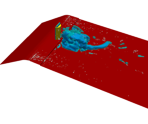
Among the stated features, the wide range of temporal and spatial scales is one of the most common sources of numerical challenges. For instance, the duration of the final stage of bubble or cavitating vortex collapse is of the order of one microsecond (Franc & Michel Reference Franc and Michel2006), while the erosion process might take place over the lifetime of a propeller. Similarly, the cavity size ranges from micro-bubbles to supercavities that span over the whole suction side of a propeller blade. Furthermore, the vapour structures can have different topologies. As an example, figure 1 shows two types of cavity topologies with different length scales on the suction side of a hydrofoil. This top-view image is extracted from the study by Foeth & van Terwisga (Reference Foeth and van Terwisga2006) on the Twist11 hydrofoil. In this typical flow, a sheet cavity is well-developed on the leading edge, while further downstream, we observe an earlier shed cavity that is collapsing. While the sheet cavity is a large mixture of liquid and vapour, which can be considered as a single continuous pseudo-fluid separated from the main liquid by an interface, the downstream cavity is in fact a cloud of sparse bubbles and very small mixture cavities which are dispersed in the liquid. A common issue in cavitation CFD is to find a suitable method to simultaneously resolve (separated) large mixture regions and capture (disperse) small-scale vapour structures. It is important to note that the correct prediction and analysis of small-scale cavities can be as important as that of large-scale structures, because cavitation initiates from micro-nuclei and usually the resulting noise, erosion, pressure shocks and strong vibrations occur at the last stages of cavity collapse at the small time and length scales.
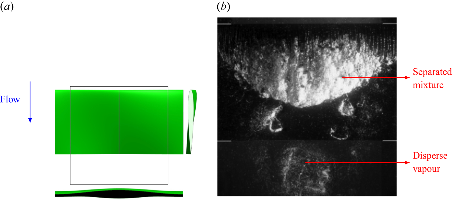
Figure 1. (a) Top, side and front view of the Twist11 hydrofoil. The black outline indicates the viewing area. (b) Different cavity topologies and length scales over the hydrofoil (top view). The images are taken from the paper by Foeth & van Terwisga (Reference Foeth and van Terwisga2006).
Most of the commonly used numerical models in engineering applications can be considered as homogeneous mixture models, which includes equilibrium and transport equation models (TEM). In the homogeneous mixture approach, the mixture of constituent phases is assumed to be a single fluid with no resolved liquid–vapour interface in each cell. Earlier studies have shown sufficient estimation of the shape of large vapour structures for different cavitating flows such as a sheet cavity on a hydrofoil (e.g. Asnaghi, Svennberg & Bensow Reference Asnaghi, Svennberg and Bensow2018b), over a convergent–divergent wedge (e.g. Budich, Schmidt & Adams Reference Budich, Schmidt and Adams2018) and fully cylindrical bluff bodies (e.g. Gnanaskandan & Mahesh Reference Gnanaskandan and Mahesh2016). However, the captured liquid–vapour interface is rather diffuse in these models and high grid resolutions with very small time steps are needed for adequate prediction of a sharp interface or to capture small structures. Most often, the cavitation/condensation is estimated based on the flow pressure, and other parameters, such as dissolved gas pressure, surface tension and viscous forces, are neglected in these models. In the equilibrium models, the pressure is related to the density and hence mixture state through an equation of state. In a TEM, a transport equation is solved for vapour volume/mass fraction and the mass transfer rate is usually adjusted through a finite mass transfer source term in this equation. The source term is usually based on the difference between flow pressure and a threshold value for the saturated vapour pressure.
The most common mass transfer models in the literature (e.g. Merkle, Feng & Buelow Reference Merkle, Feng and Buelow1998; Kunz et al. Reference Kunz, Boger, Stinebring, Chyczewski, Lindau, Gibeling, Venkateswaran and Govindan2000; Schnerr & Sauer Reference Schnerr and Sauer2001) can be interpreted as a simplified form of the Rayleigh–Plesset equation in which the mentioned parameters, as well as the bubble inertia, are neglected. As a result, these mass transfer models cannot appropriately resolve the dynamics of small collapsing cavities, especially sparse clouds of bubbles (figure 1b). As an example, Asnaghi, Feymark & Bensow (Reference Asnaghi, Feymark and Bensow2018a) observed that the rate of phase change from vapour to liquid is over-predicted for a shed cloud on the suction side of a hydrofoil, which leads to an early collapse of the cloud in numerical modelling. Ye & Li (Reference Ye and Li2016) showed that the bubble growth rate can be greatly reduced if the bubble–bubble interaction and second-order derivative in the Rayleigh–Plesset equation are considered. Moreover, homogeneous models cannot resolve the very small nuclei, which are fundamentally assumed to be the cavitation starting points. Consequently, these models are limited in an appropriate prediction of cavitation inception. For example, in the modelling of bluff body cavitation by Gnanaskandan & Mahesh (Reference Gnanaskandan and Mahesh2016), the numerical inception point is upstream of the separation point, because cavitation was assumed to occur as soon as the pressure drops below the vapour pressure. However, in corresponding experimental studies (e.g. Arakeri Reference Arakeri1975), cavitation does not occur immediately at the location where the pressure drops below the vapour pressure, but instead occurs downstream of the separation point. Therefore, it can be stated that while homogeneous mixture models are suitable options for representing large mixture regions, cavity structures smaller than the grid size, such as cavitation nuclei and bubbles, or sparse clouds of bubbles, are not well treated using these approaches. This results from the simplifications in modelling the phase change rate as well as the spatial and temporal resolution dependencies. Accurate simulation of sub-grid structures and their violent collapses and fast rebounds are crucial in the proper prediction of cavitation consequences. As the governing equations of the homogeneous mixture models are solved in the Eulerian framework (similar to the continuity and momentum equations), in this paper, we call them Eulerian models.
Apart from the widely used homogeneous mixture models, Lagrangian models can address some of the above-mentioned limitations. Here, the continuous liquid properties are calculated using Eulerian conservation equations, whereas the vapour part is governed by Newtonian motion of individual spherical bubbles or parcels of bubbles in the Lagrangian framework. Owing to numerical limitations, these models have been less popular in cavitation modelling, however, they offer desirable features which make them the most eligible options for special cases. The Lagrangian bubble models enable the consideration of a large number effects that are deemed important for high-fidelity predictions of the smallest scales in cavitation phenomena, such as the effects of dissolved gas, liquid surface tension and viscous tension, and accounting for bubble–bubble and bubble–wall interactions and turbulence effects on bubble motion and break-up. Because different flow forces on cavities are implemented directly in the transport equation and the bubble size variation is estimated using a more complete form of the Rayleigh–Plesset equation, Lagrangian models can give a more realistic estimation of cavitation dynamics, especially for small-scale structures. In fact, cavitation inception studies are often performed using the discrete Lagrangian approach. Furthermore, using different bubble number/size spectra for the liquid provides access to the liquid (e.g. water) quality effects, which is considered another major advantage of Lagrangian cavitation models.
These models have been extensively used in the literature for simulation of clusters of bubbles, especially with a dilute suspension. For example, Fuster & Colonius (Reference Fuster and Colonius2011) proposed a Lagrangian formulation for bubbly flows based on the volume-averaged approach in which the continuum phase is solved from the averaged equations for the mixture (similar to the homogeneous mixture models), while the influence of the dispersed phase is treated as source terms in the continuity, momentum and energy equations. The Lagrangian models can also be suitable tools for small-scale applications, such as medical applications, in which the cavity length scale is approximately  $1\ \mathrm {\mu }\textrm {m} \sim 1\ \textrm {mm}$ and the interaction between pressure waves and bubbles are of great importance. As an example, Maeda et al. (Reference Maeda, Colonius, Kreider, Maxwell and Bailey2016) simulated the interactions between bubble clouds and ultrasound pulses to model burst-wave lithotripsy, a method that uses focused ultrasound pulses to fragment kidney stones. There are also a few studies in the literature that apply Lagrangian modelling in real-case industrial problems at larger scales. For instance, Giannadakis, Gavaises & Arcoumanis (Reference Giannadakis, Gavaises and Arcoumanis2008) presented a stochastic Lagrangian model to simulate the onset and development of cavitation inside diesel nozzle holes. However, the Lagrangian models can be computationally expensive when the number of bubbles is large. Furthermore, Lagrangian models are limited in the representation of large and non-spherical vapour pockets, which are not well-represented by the solution of the Rayleigh–Plesset equation. As explained earlier, Eulerian mixture models are more suitable options for such structures. Therefore, considering the cavity categorization based on the length scale (depicted in figure 1), we see that for a group of cavities, Eulerian mixture models are more suitable and Lagrangian bubble models suffer from theoretical/computational limitations, while the reverse case applies for the other cavity group, so finding an appropriate model that efficiently resolves both topologies is an issue.
A solution to this problem can be a hybrid model in which large cavity structures are modelled using an Eulerian mixture model, while small sub-grid structures as well as sparse bubble clusters are tracked as Lagrangian bubbles. Hybrid Eulerian–Lagrangian solvers have gained more popularity in recent years for simulation of multi-scale applications such as atomizing gas–liquid flows (e.g. Kim, Herrmann & Moin Reference Kim, Herrmann and Moin2006; Herrmann Reference Herrmann2010; Tomar et al. Reference Tomar, Fuster, Zaleski and Popinet2010; Ström et al. Reference Ström, Sasic, Holm-Christensen and Shah2016). A good example of a hybrid cavitation model is the work of Hsiao, Ma & Chahine (Reference Hsiao, Ma and Chahine2017), who coupled a Lagrangian discrete singularities model with an Eulerian level-set approach using the ghost-fluid method. In the applied level-set model, the mass transfer between the two phases is not taken into account. Instead, tracking of the Lagrangian bubble motion and the resulting concentration field provides the vapour volume fraction and mixture density. In the hybrid model, natural free field nuclei and solid boundary nucleation are used in the representation of cavitation inception and enable capture of the sheet and cloud dynamics. The method is shown to be in good agreement with two-dimensional (2-D) experimental measurements in terms of sheet cavity lengths and shedding frequency, however, it has not been validated with a three-dimensional (3-D) case and, according to the authors, the results do not yet show clear cloud shedding which is assumed to arise from an inadequate grid resolution. Numerical stability and compatibility between the two frameworks can be major issues in developing hybrid cavitation methods. Hence, the earlier hybrid models include simplifications in the Lagrangian representation and Eulerian–Lagrangian transition algorithm, which can lead to other numerical issues. Some of these issues, which cause spurious pressure pulses in the flow field, have been addressed in an earlier study (Ghahramani, Arabnejad & Bensow Reference Ghahramani, Arabnejad and Bensow2018).
Based on our earlier experience, the Eulerian mixture model is limited in capturing the small-scale cavity dynamics, especially during cavitation inception and collapse of shedding clouds (see e.g. Asnaghi et al. Reference Asnaghi, Feymark and Bensow2018a). In a recent study (Ghahramani et al. Reference Ghahramani, Jahangir, Neuhauser, Bourgeois, Poelma and Bensow2020), the Eulerian model simulation could not sufficiently capture the cavity development in a multi-scale flow around a bluff body. The investigated bluff body is a surface-mounted semi-circular cylinder, which generates various cavity structures of different length scales. Based on our experimental tests and the work of Escaler et al. (Reference Escaler, Farhat, Avellan and Egusquiza2003), the cavity structures around this cylinder can have aggressive collapses, which are highly erosive at high flow rates, and it is desirable to obtain further understanding and a detailed analysis of this complex flow from numerical simulation. To overcome the limitations with the Eulerian model, in the current study, we develop a new hybrid solver by coupling the Eulerian model with a Lagrangian model. The Lagrangian cavitation model, which has been developed in a recent study (Ghahramani, Arabnejad & Bensow Reference Ghahramani, Arabnejad and Bensow2019), is capable of tracking individual bubbles and resolving their dynamics based on an improved localized form of the Rayleigh–Plesset equation. The model has been verified with benchmark test cases including the collapse of a single bubble and a cluster of bubbles. Additionally, the Eulerian model is a transport equation model based on liquid volume fraction, in which the mass transfer between the liquid and vapour is taken into account by a finite source term in the equation. Furthermore, cavitation is initiated in low pressure regions, owing to the mass transfer, and initial sub-grid cavities are transformed to the Lagrangian framework to improve the prediction accuracy of the growth of small bubbles. Using the hybrid Eulerian mixture–Lagrangian bubble solver, we then analyse the multi-scale cavitating flow around the bluff body by both modelling the large-scale cavities and capturing the sub-grid vapour structures.
In developing the hybrid solver, our Lagrangian model is further improved in this study to be applicable in 3-D real test cases at large scales. Additionally, we use an algorithm for the coupling of the two frameworks and the transition of small-scale Eulerian structures to the Lagrangian framework and vice versa. The transition algorithm is, in basic principles, similar to that developed by Vallier (Reference Vallier2013), which was followed by Lidtke (Reference Lidtke2017) for the prediction of radiated noise and recently by Peters & El Moctar (Reference Peters and El Moctar2020) for an estimation of cavitation-induced erosion. It can be shown that the algorithm, in its original form that has been used earlier, does not follow the conservation laws for mass, momentum and kinetic energy in a cavitating flow. This, in turn, can induce spurious pressure pulses and vapour generation, and lead to solution instability and numerical errors in the noise and erosion estimation. In the current model, however, the algorithm is improved to follow the conservation laws and avoid the numerical issues, as will be discussed in the following sections. The current hybrid model includes further improvements, compared with earlier models, such as implementing new submodels to consider bubble–bubble interactions and break-up, introducing bubble parcels, and revising the bubble–wall boundary condition and the void handling scheme. The solver is developed in the open source C++ package OpenFOAM.
From the obtained numerical results, the multi-scale cavity development is discussed in detail, which gives new insights on the flow physics that have not been otherwise detectable from high-speed images of the experimental test. Although, from the experimental result, we can identify cyclic cavity shedding from the wake area behind the bluff body, it is not possible to explain the cavity development in each cycle using only the high-speed images. The numerical results clarify various interactions between the large- and small-scale cavities as well as the continuous flow. It is shown that small-scale cavities not only are important at the inception and collapse steps, but also influence the development of large-scale structures. Furthermore, the effects of various parameters on the cavity dynamics are explained, which include the flow vorticity, pressure variation rate, bubble inertia and surface tension effects.
We continue to provide a general description of the hybrid solver in § 2 and explain how the Eulerian mixture and Lagrangian bubble models are coupled in the solution algorithm. Then the details of the models, which include the developed and applied submodels, governing equations and the Eulerian–Lagrangian transition algorithm, are presented in § 3. Afterwards, the multi-scale problem of a periodic cavitating flow behind a bluff body is described, which is followed by validating the hybrid model performance in § 4. Subsequently, we analyse multi-scale cavitation using the obtained numerical results in § 5. The paper is finally concluded with recommendations for future studies in § 6.
2. Methodology
In figure 2, the general solution algorithm is described schematically. In the hybrid model, the large vapour structures are modelled through the Eulerian mixture approach and the small-scale structures are represented as discrete parcels of bubbles. The governing equations of the continuous flow field (i.e. the conservation equations for mass and momentum) are the same for both and the main difference is in the tracking of the cavity structures. Here, the cavities are categorized as Eulerian structures and Lagrangian bubbles to be tracked in the corresponding framework. The categorization into Lagrangian and Eulerian groups is done based on the relative size of each cavity to the local grid size of the discretized domain. If a cavity is large enough to be resolved by a sufficient number of computational cells, then it is tracked in the Eulerian framework, otherwise it is treated as parcels of Lagrangian bubbles. Furthermore, because the volume of each cavity can change in the flow, at each time step, the small Eulerian structures or large Lagrangian cavities may be transformed from one framework to the other.
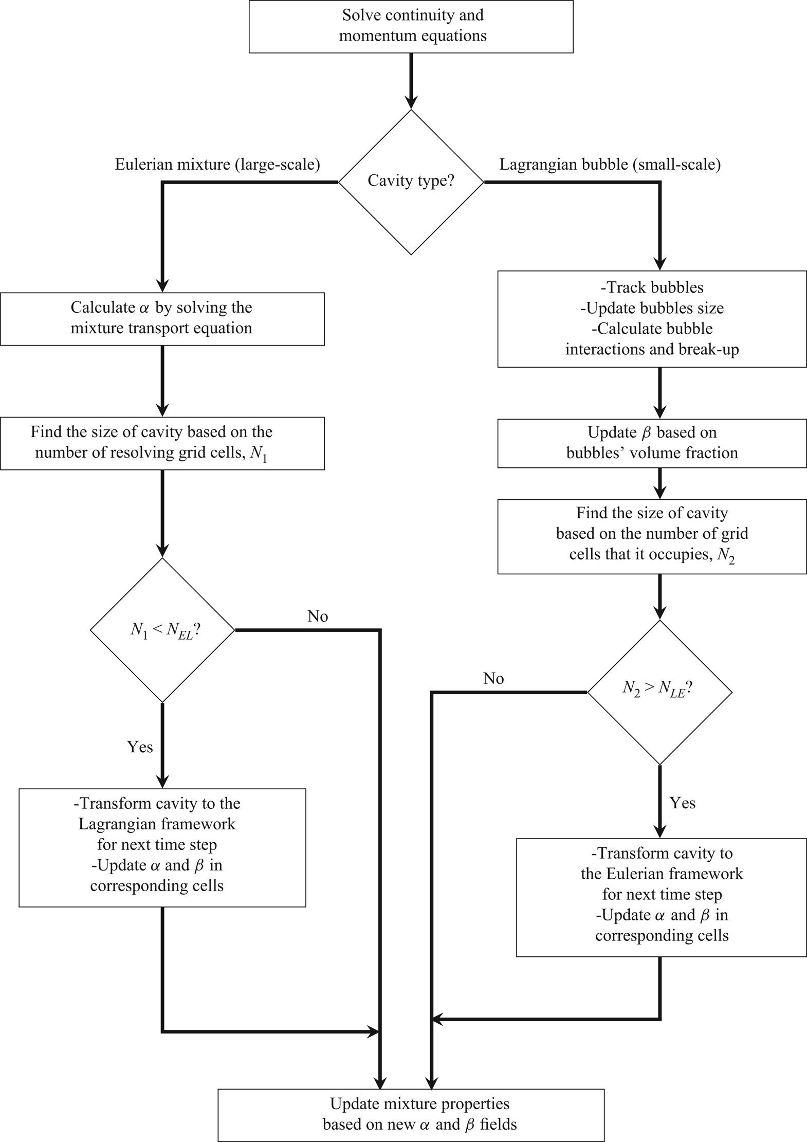
Figure 2. Schematic description of a time step in the general solution algorithm.
In the Eulerian modelling, the mixture of vapour and liquid phases is treated as a single mixture fluid, where the continuity equation and one set of momentum equations for the mixture are solved. We here consider an incompressible flow and a TEM, motivated by the balance of computational cost and model accuracy for the large-scale applications, as will be shown later, but a similar framework can be developed for compressible flows. By solving the transport equation, we obtain the liquid volume fraction (denoted by  $\alpha$), which is used to update the mixture properties (e.g. density).
In the Lagrangian modelling, the cavities are treated as discrete parcels of bubbles in an ambient Eulerian continuous flow. At each time step, the Eulerian continuity and momentum equations are solved first, then the bubbles are tracked by solving a set of ordinary differential equations along the trajectory of the bubble. Afterwards, the bubble dynamics is updated and its interactions with the other cavities are modelled. Then the Eulerian vapour fraction is updated based on the new positions and radii of the bubbles. The vapour fraction is used to update the mixture properties (e.g. density) and consider the bubble effect on the ambient flow.
For updating the mixture properties based on liquid and vapour fractions, it is important to note that the vapour content of each cell is represented by either Eulerian or Lagrangian models. Therefore, it is assumed that Eulerian and Lagrangian cavities do not co-exist in the same cell. To distinguish between the obtained volume fraction from bubble distribution and that calculated from the Eulerian transport equation model ( $\alpha$), we use another variable,
  $\beta$, for Lagrangian cavities. In a similar way,
  $\beta$ is used to update the properties of the liquid–vapour mixture in the Eulerian governing equations, as will be explained in detail in § 3.2. It should also be noted that because we have both Eulerian and Lagrangian cavities in the hybrid model, the governing equations of the continuous flow field should be revised accordingly to include both
  $\alpha$ and
  $\beta$, and this is described is § 3.3.
Furthermore, the solution algorithm needs a procedure for transition of small Eulerian cavities to the Lagrangian framework and vice versa. This procedure includes two parts: a criterion to determine when a cavity should be transformed from one framework to the other; and an algorithm which specifies how such a transition should be performed. For the transition criterion, similar to the other hybrid models, we consider two threshold numbers related to the size of the cavity in relation to the grid:  $N_{EL}$ for Eulerian to Lagrangian transformation; and
  $N_{LE}$ for Lagrangian to Eulerian transformation (figure 2). If an Eulerian cavity is represented by a sufficient number of computational cells which is larger than
  $N_{EL}$, then it is kept in the Eulerian framework, otherwise it is determined to be insufficiently resolved and transformed to a group of Lagrangian bubbles. However, if a Lagrangian cavity (i.e. a cloud of Lagrangian bubbles) is large enough and occupies more than
  $N_{LE}$ cells, then it is transformed to the Eulerian framework, as it can be resolved by a sufficient number of cells, otherwise it is kept in the Lagrangian framework. The two threshold numbers are different and
  $N_{LE} > N_{EL}$, so that when a small Eulerian cavity is transformed to a group of Lagrangian bubbles, its (possibly) fast collapse and rebound process can be modelled using the Lagrangian equations, instead of having a quick transformation back to the Eulerian framework.
How the Eulerian–Lagrangian transition is performed is similar to the algorithm developed by Vallier (Reference Vallier2013). That algorithm was in turn inspired by the model of Tomar et al. (Reference Tomar, Fuster, Zaleski and Popinet2010) for atomizing flows and therefore it should be improved for cavitation modelling. There are important distinctions between the flow characteristics in cavitation and atomization. In atomized liquids, it is possible to replace each liquid fragment with one Lagrangian droplet with equal volume (as done by Tomar et al. Reference Tomar, Fuster, Zaleski and Popinet2010), while in cavitating flows, each Eulerian structure is actually a cloud of bubbles and its properties (e.g. density) are not equal to the pure vapour properties. Therefore, each Eulerian cavity should be replaced by a group of smaller bubbles (instead of one larger bubble) in such a way that the properties of the combined bubble group are equal to the corresponding values of the Eulerian structure. Furthermore, the bubble effect should be considered in the mixture properties as well mass transfer rate between the two phases. Otherwise the physical conservation laws are not followed and we may have numerical instabilities and spurious pressure pulses in the solution. These issues have been explained in detail and addressed in an earlier study (Ghahramani et al. Reference Ghahramani, Arabnejad and Bensow2018). In the revised algorithm, each Eulerian cavity is replaced by a group of smaller bubbles and the bubble effect in the mixture properties, and mass transfer rate is considered through the introduction of the  $\beta$ parameter and the revision of the governing equations, as will be described in § 3.
In the current study, the algorithm is improved further to be applicable to real-case 3-D flows. As will be explained in § 3, the improved transition process is compatible with the flow physics and the mass, momentum and kinetic energy of the cavities are conserved during the process, contrary to the previously mentioned studies. Another new improvement is the correction of the bubble wall boundary condition, which is important in the transport of large bubbles. Furthermore, in the hybrid model, the bubble size is updated by solving a new localized form of the Rayleigh–Plesset equation, which takes into account the local pressure effect on bubble dynamics. The bubble–bubble interaction is also improved in this study both to follow the physical conservation laws and to considerably increase the computational efficiency. The other new contributions are revising the void handling scheme and implementing another submodel to consider the bubble break-up arising from the flow turbulence and velocity fluctuations. Detailed description of the stated features is given in § 3.
3. Numerical models
In §§ 3.1 and 3.2, we describe the Eulerian and Lagrangian models and their governing equations. Then, in § 3.3, we explain how these two models are coupled with each other in the hybrid model and how the governing equations are revised accordingly.
3.1. Homogeneous mixture model
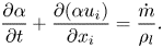
In the transport equation model, the liquid–vapour mixture is represented by solving a scalar transport equation for the liquid volume fraction, where the mass transfer between the phases is defined as an explicit source term in the equation and surface tension effects are assumed to be small and are neglected. The governing equations are Favre-averaged and then spatially filtered to perform large eddy simulation (LES). Turbulence is modelled using an implicit large eddy simulation (ILES) approach. The unfiltered continuity and momentum equations are
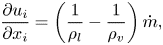 $$\begin{gather} \frac{\partial u_i}{\partial x_i } = \left(\frac{1}{\rho_l}-\frac{1}{\rho_v}\right){\dot{m}}, \end{gather}$$
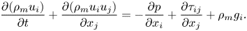 $$\begin{gather}\frac{\partial (\rho_m u_i)}{\partial t} + \frac{\partial (\rho_m u_i u_j)}{\partial x_j } ={-}\frac{\partial p}{\partial x_i}+\frac{\partial \tau_{ij}}{\partial x_j} + \rho_m g_i. \end{gather}$$
The right-hand side term of the continuity equation describes the effect of vaporization and condensation, where  $\rho _l$ is the liquid density,
  $\rho _v$ is the vapour density and
  $\dot {m}$ is the rate of mass transfer between phases, and is obtained from a finite mass transfer (FMT) model. In the ILES approach, the numerical dissipation is considered as sufficient to mimic the sub-grid terms (Drikakis et al. Reference Drikakis, Hahn, Mosedale and Thornber2009; Bensow & Bark Reference Bensow and Bark2010). Additionally,
  $\rho _m$ and
  $\tau _{ij}$ are the mixture density and the viscous stress tensor, respectively, which are defined as
 $$\begin{gather} \rho_m = \alpha \rho_l + (1-\alpha) \rho_v , \end{gather}$$
 $$\begin{gather}\tau_{ij}= \mu_m \left( \frac{\partial u_i}{\partial x_j} + \frac{\partial u_j}{\partial x_i} - \frac{2}{3} \frac{\partial u_k}{\partial x_k} \delta_{ij} \right), \end{gather}$$
where the pure phase densities are assumed to be constant in the incompressible modelling, and  $\mu _m$ is the mixture dynamic viscosity given by
 \begin{equation} \mu_m = \alpha \mu_l + (1-\alpha) \mu_v. \end{equation}
Here,  $\alpha$ is the liquid volume fraction, which specifies the relative amount of liquid in a given volume, e.g. a computational cell. In this model, the evolution of the volume fraction is calculated by solving a scalar transport equation given as
 \begin{equation} \frac{\partial \alpha}{\partial t} + \frac{\partial (\alpha u_i)}{\partial x_i } = \frac{\dot{m}}{\rho_l}. \end{equation}
To close the above set of equations, the mass transfer rate,  $\dot {m}$, should be specified using an FMT model. There are many numerical models in the literature that can be used to estimate this term and most of them are based on a simplified form of the well-known Rayleigh–Plesset equation. In this study, the Schnerr–Sauer model (Schnerr & Sauer Reference Schnerr and Sauer2001) is used, which has been proven in earlier studies to give satisfactory results with reasonable computational cost (see e.g. Asnaghi et al. Reference Asnaghi, Svennberg and Bensow2018b). The vaporization and condensation rates are then given by
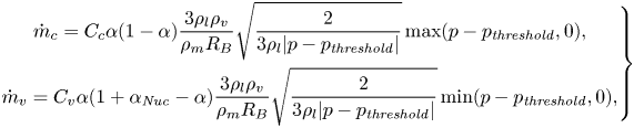 \begin{equation} \left.\begin{gathered} \dot{m}_c = C_c \alpha(1 - \alpha) \frac{3 \rho_l \rho_v}{\rho_m R_B}\sqrt{\frac{2}{3\rho_l |p - p_{\mathit{threshold}}|}} \max(p - p_{\mathit{threshold}}, 0),\\ \dot{m}_v = C_v \alpha(1 + \alpha_{\mathit{Nuc}} - \alpha) \frac{3 \rho_l \rho_v}{\rho_m R_B}\sqrt{\frac{2}{3\rho_l |p - p_{\mathit{threshold}}|}} \min(p - p_{\mathit{threshold}}, 0), \end{gathered}\right\} \end{equation}
where  $\dot {m}_c$ and
  $\dot {m}_v$ are the rates of condensation and vaporization, respectively, and
  $\dot {m} = \dot {m}_c + \dot {m}_v$. In the above equations,
  $R_B$ and
  $\alpha _{\mathit {Nuc}}$ are the generic radius and volume fraction of bubble nuclei in the liquid, which are obtained from
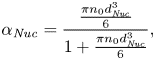 $$\begin{gather} \alpha_{\mathit{Nuc}}= \frac{\frac{\pi n_0 d_{\mathit{Nuc}}^3}{6}}{1+\frac{\pi n_0 d_{\mathit{Nuc}}^3}{6}}, \end{gather}$$
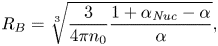 $$\begin{gather}R_B = \sqrt[3]{\frac{3}{4\pi n_0}\frac{1+\alpha_{\mathit{Nuc}}-\alpha}{\alpha}} , \end{gather}$$
where  $n_0$ and
  $d_{\mathit {Nuc}}$ are user-defined parameters corresponding to the number of nuclei per liquid cubic meter and the nucleation site diameter, respectively, and they are assumed to be
  $10^{10}$ m
 $^{-3}$ and
  $10^{-5}$ m. Here,
  $C_c$ and
  $C_v$ are the condensation and vaporization rate coefficients in OpenFOAM (OpenFoam 2018). It should be mentioned that the overall effect of the empirical parameters,
  $n_0$,
  $d_{\mathit {Nuc}}$,
  $C_c$ and
  $C_v$, are two constant numbers in the condensation and vaporization source terms, and they can be set to different reasonable values. Based on our earlier experience, using larger empirical constants leads to more satisfactory results (Ghahramani et al. Reference Ghahramani, Arabnejad and Bensow2019) and sufficiently large mass flow rates can mimic a barotropic equation of state (Schenke & van Terwisga Reference Schenke and van Terwisga2017). Furthermore, it has been observed that in simulating cavitating flows, the vaporization coefficient should be large, in principle as high as possible without compromising numerical stability, to satisfy near instantaneous evaporation, while the smaller condensation coefficient allows for some retardation in the condensation (Wikstrom, Bark & Fureby Reference Wikstrom, Bark and Fureby2003). Accordingly, the vaporization constant is modified as
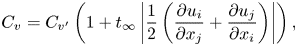 \begin{equation} C_v = C_{v'}\left(1 + t_{\infty}\left| \frac{1}{2} \left(\frac{\partial u_i}{\partial x_j} + \frac{\partial u_j}{\partial x_i} \right) \right|\right), \end{equation}
where  $t_{\infty } = L/U_{\infty }$ is the time scale of the mean flow used to normalize the velocity strain rate value (Asnaghi et al. Reference Asnaghi, Feymark and Bensow2018a). In this study,
  $C_c$ and
  $C_{v'}$ are set to 10. In (3.7),
  $p_{\mathit {threshold}}$ is a threshold pressure at which the phase change is assumed to happen, usually considered as the vapour pressure of the fluid, which is 2320 Pa in the current simulations. Finally, the liquid and vapour densities are assumed to be
  $\rho _l = 998.85$ kg m
 $^{-3}$ and
  $\rho _v = 0.02$ kg m
 $^{-3}$, and the corresponding dynamic viscosity values are set as
  $\mu _l = 0.00109$ kg m
 $^{-1}$ s
 $^{-1}$ and
  $\mu _v = 1.39\times 10^{-5}$ kg m
 $^{-1}$ s
 $^{-1}$.
From the equations, it is seen that the mass transfer rate model neglects the effects of dissolved gas pressure, surface tension and viscous force.
3.2. Lagrangian bubble model
As stated before for this model, at each time step, the Eulerian equations are solved first, then the bubbles are tracked by solving a set of ordinary differential equations along the trajectory of the bubble, after which the Eulerian vapour fraction is updated based on the new positions and radii of the bubbles. The Eulerian governing equations are the continuity and Navier–Stokes equations, as described for the Eulerian mixture model ((3.1) and (3.2)). To avoid high computational costs, instead of modelling all of the bubbles, parcels of them are tracked. Each parcel represents a number of identical non-interacting bubbles, which are assumed to be spherical. There are a few other inherent assumptions that will be described in the following sections.
In Lagrangian modelling, various flow effects are modelled through different models and the main aim of this section is to introduce the submodels in bubble modelling. However, for the interested reader, further details and assumptions about some of following submodels are given in Appendix A. This appendix also includes the rationale behind developing or choosing the following submodels and brief comparisons with other available models in the literature.
3.2.1. Bubble effect on the Eulerian flow field
Because the dispersed (bubble) phase in the cavitating flow is locally dense and has properties quite different from liquid properties, the bubbles have a considerable effect on the ambient flow field (similar to Eulerian cavities) as well as other bubbles. Thus, both the bubble–bubble and bubble–flow interactions should be considered in the model. The bubble–flow interaction can be implemented in the Eulerian equations in different ways which, to a large extent, define the characteristics of the Lagrangian/hybrid model (Ghahramani et al. Reference Ghahramani, Arabnejad and Bensow2018). In this study, the bubble effect is considered by implementing its volume fraction contribution in the calculation of mixture properties and phase change rate ((3.3), (3.5) and (3.7)), similar to the described finite mass transfer model (§ 3.1). In this approach, the flow is considered as a single fluid mixture of continuous liquid and disperse bubbles, and the Eulerian governing equations are similar to the homogeneous mixture model. However, the liquid volume fraction of each cell is obtained from bubble cell occupancy instead of solving the scalar transport equation (3.6). Therefore, for the Lagrangian model the mixture properties are given as
 \begin{equation} \rho_m = \beta \rho_l + (1-\beta) \rho_v , \quad \mu_m = \beta \mu_l + (1-\beta) \mu_v, \end{equation}
where  $\beta$ is the liquid volume fraction and simply
  $1 - \beta$ is the bubble volume fraction in the computational cell. A comparison of (3.3), (3.5) and (3.11a,b) shows that for Lagrangian modelling,
  $\beta$ just replaces
  $\alpha$, and it is important to remember that there is no Eulerian cavity in this model. In the Lagrangian model of Fuster & Colonius (Reference Fuster and Colonius2011), as well as the hybrid model of Hsiao et al. (Reference Hsiao, Ma and Chahine2017), the effect of the bubbles on the ambient flow field is considered in the same way. It should be mentioned that the continuity equation source term is obtained using the Schnerr–Sauer model (3.7), similar to the mixture model. It is possible to calculate the phase change source term from the bubble size and distribution variation directly; however, as the main intention is to use the Lagrangian approach coupled to an FMT-based model, the Schnerr–Sauer model is preferred here.
The remaining part is to calculate the vapour volume fraction from the instantaneous bubble sizes and locations. In the general case, a cavitating bubble may grow and occupy more than one grid cell. If we assume that a bubble parcel  $i$ is occupying
  $N_{\textit {cell}}$ cells, then the void fraction of the parcel in cell
  $j$ can be estimated as
 \begin{equation} v_{i,j} = \frac{1}{V_{\mathit{cell},j}}\left(\frac{4}{3}\pi n_i R^3_i\right) f\left(\frac{|\boldsymbol{x}_{i,j}|}{R_i}\right), \end{equation}
in which  $R_i$ is the radius of the bubble,
  $n_i$ is the number of bubbles that the parcel represents,
  $f(|\boldsymbol {x}_{i,j}|/{R_i})$ is the Gaussian distribution function, and
  $|\boldsymbol {x}_{i,j}|$ is the distance between the cell and parcel centre. The cells that are included in the formula are located around the host cell of the bubble and they are partially or fully occupied by the parcel, and the volume of the parcel is not distributed over the unoccupied neighbouring cells. The standard deviation of the distribution function is calibrated so that
  $99.7\,\%$ of the bubble volume is distributed within the
  $|\boldsymbol {x}_{i,j}| < R_i$ range. Because (3.12) does not necessarily guarantee that the volume of the parcel is conserved, the void fraction should be corrected as
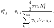 \begin{equation} v^c_{i,j} = v_{i,j}\frac{\dfrac{4}{3}\pi n_i R^3_i}{\displaystyle\sum_{k=1}^{N_{\mathit{cell}}}v_{i,k}V_{\mathit{cell},k}}. \end{equation}
Finally, as a cell can be occupied by  $N_b > 1$ parcels, the vapour void fraction of cell
  $j$ is the summation of all the void fractions of the bubbles, given as
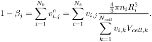 \begin{equation} 1 - \beta_j = \sum_{i=1}^{N_{b}}v^c_{i,j} = \sum_{i=1}^{N_{b}}v_{i,j}\frac{\frac{4}{3}\pi n_i R^3_i}{\displaystyle\sum_{k=1}^{N_{\mathit{cell}}}v_{i,k}V_{\mathit{cell},k}}. \end{equation}
 In cavitating flows, bubbles may experience a significant pressure drop within a short distance, which can result in a substantial growth. Therefore, it is possible that some parcels become larger than the fine hosting cells. One of the inherent assumptions in Lagrangian modelling is that the dispersed-phase volume fraction should not be too high. Theoretical problems arise at the limit of very low values of  $\beta$. Another situation with high Lagrangian vapour fraction is in the locally dense regions, where a cell hosts a large number of bubbles. When the presence of Lagrangian bubbles approaches the packing limit, overpacking should be prevented, otherwise it can lead to unphysical results and the risk of crashing the solver. In this study, the maximum value of bubble volume fraction was limited to 0.64 (or
  $\beta _{min} = 0.36$), which is a relevant number corresponding to a random close packing limit of monodispersed spheres. Therefore, the bubble volume fraction in each computational cell is calculated using (3.14), and for the overpacked cells, it is distributed to the neighbouring cells. It should be mentioned that this case does not happen frequently in the hybrid solver, because dense Lagrangian cavities are usually transformed to the Eulerian framework, as will be shown later. In the extreme case when a bubble is larger than the surrounding cells, it is enough to spread its volume over an approximate radial distance of
  $1.16R = {(\frac {1}{0.64})}^{{1}/{3}} R$. Distribution of the bubble volume over only the neighbouring cells that are occupied by the cavitating bubbles gives a more precise estimation of the real concentration field compared with some of the earlier studies (e.g. Fuster & Colonius Reference Fuster and Colonius2011; Vallier Reference Vallier2013; Hsiao et al. Reference Hsiao, Ma and Chahine2017) in which the bubble volume is spread within a larger radial distance, e.g.
  $3R$.
$3R$.
3.2.2. Bubble equations of motion
The Lagrangian equations for tracing bubbles are given by
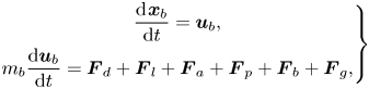 \begin{equation} \left.\begin{gathered} \frac{\textrm{d}\kern0.06em \boldsymbol{x}_{b}}{\textrm{d}t} = \boldsymbol{u}_{b} ,\\ m_b \frac{\textrm{d}\boldsymbol{u}_{b}}{\textrm{d}t} = \boldsymbol{F}_d + \boldsymbol{F}_l + \boldsymbol{F}_a + \boldsymbol{F}_p + \boldsymbol{F}_b + \boldsymbol{F}_g , \end{gathered}\right\} \end{equation}
where  $\boldsymbol {x}_{b}$ and
  $\boldsymbol {u}_{b}$ denote the position and velocity vectors of the bubble, and
  $m_b$ is the mass of the bubble. The right-hand side of the second equation includes various force components exerted on the bubbles. Explicit implementation of flow forces is an advantage of the Lagrangian model, which gives the opportunity to consider different flow effects on cavity behaviour, but it also means that the representation is dependent on the accuracy of available models for these effects. The listed forces in the equation are, from left to right, sphere drag force, lift force, added mass, pressure gradient force, buoyancy force and gravity. These forces are given as
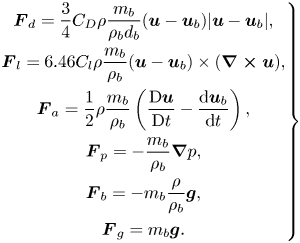 \begin{equation} \left.\begin{gathered} \boldsymbol{F}_d = \frac{3}{4}C_D\rho\frac{m_b}{\rho_b d_b}(\boldsymbol{u} - \boldsymbol{u}_{b})|\boldsymbol{u} - \boldsymbol{u}_{b}|, \\ \boldsymbol{F}_l = 6.46 C_{l} \rho \frac{m_b}{\rho_b}(\boldsymbol{u} - \boldsymbol{u}_{b})\times(\boldsymbol{\nabla\times u}), \\ \boldsymbol{F}_a= \frac{1}{2}\rho\frac{m_b}{\rho_b}\left(\frac{\textrm{D}\boldsymbol{u}}{\textrm{D}t} - \frac{\textrm{d}\boldsymbol{u}_{b}}{\textrm{d}t} \right),\\ \boldsymbol{F}_p={-}\frac{m_b}{\rho_b}\boldsymbol{\nabla} p,\\ \boldsymbol{F}_b ={-}m_b\frac{\rho}{\rho_b} \boldsymbol{g},\\ \boldsymbol{F}_g = m_b \boldsymbol{g}. \end{gathered}\right\} \end{equation}
In these relations,  $\rho _b$ and
  $d_b$ are the density and diameter of the bubble, and
  $\rho$ is the density of the surrounding fluid. Additionally,
  $C_D$ is the drag coefficient, which is defined as (Amsden, O'Rourke & Butler Reference Amsden, O'Rourke and Butler1989)
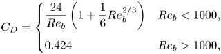 \begin{equation} C_D = \begin{cases} \dfrac{24}{Re_b}\left(1+\dfrac{1}{6}Re_b^{{2}/{3}}\right) & Re_b<1000, \\ 0.424 & Re_b>1000, \end{cases} \end{equation}
where  $Re_b$ is the bubble Reynolds number, defined as
 \begin{equation} {Re_b} = \frac{\rho d_b |\boldsymbol{u} - \boldsymbol{u}_{b}|}{\mu}. \end{equation}
Additionally, in the lift force,  $C_{l}$ is given as (Mei, Reference Mei1992)
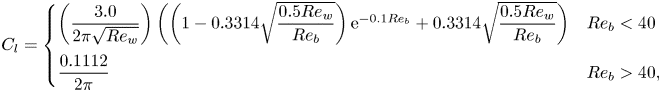 \begin{align} C_{l} = \begin{cases} \left(\dfrac{3.0}{2\pi \sqrt{Re_w}} \right) \left( \left(1-0.3314\sqrt{\dfrac{0.5Re_w}{Re_b}}\right)\textrm{e}^{{-}0.1Re_b}+ 0.3314\sqrt{\dfrac{0.5Re_w}{Re_b}}\right) & Re_b<40\\ \dfrac{0.1112}{2\pi} & Re_b>40, \end{cases} \end{align}
and  $Re_w$ is the vorticity Reynolds number, defined as
 \begin{equation} {Re_w} = \frac{\rho {d_b}^2 |\boldsymbol{\nabla\times u}|}{\mu}. \end{equation}
 Another fundamental assumption in classical Lagrangian methodologies is that the dimensions of the particles (or bubbles) under consideration should be smaller than the characteristic size of the Eulerian mesh. In fact, the maximum particle size should be such that  $5\sim 10 \ d_{max} < L$, where
  $L$ is the characteristic cell size. This assumption can be violated in cavitating flows, owing to the combination of dense grids and the growth of bubbles in low pressure regions. To circumvent this limitation, in (3.16)–(3.20), instead of interpolating the Eulerian values at the centre of the bubble, the corresponding values are averaged along the surface of a larger and concentric imaginary sphere. This sphere has a diameter of
  $5 d_b$.
In bubble transport, the wall boundaries are considered to be rigid and it is assumed that a bubble collides with a wall when the distance between its centre to the nearest wall face becomes equal or less than its radius. The applied boundary conditions are explained further in Appendix B. The other important issue in the tracking of Lagrangian bubbles that should be considered in numerical modelling is the relative sizes of bubbles and grid cells near the walls. As mentioned, sometimes a bubble may grow and occupy several cells. In OpenFOAM, and some other widely used numerical codes, when a bubble approaches a wall, the wall boundary condition is applied correctly only if the bubble size is smaller than the cell edge in the wall normal direction. If a bubble is larger than this limit, the bubble–wall collision is not detected. In the current study, the bubble wall boundary condition in OpenFOAM is improved to model the large bubble–wall collision appropriately.
The forces typically depend on the bubble size, and hence a correct estimation of bubble dynamics is of great importance.
3.2.3. Bubble dynamics
The classical Rayleigh–Plesset equation can estimate the collapse and growth rate of a single bubble in an infinite domain reasonably well (Franc & Michel Reference Franc and Michel2006). However, owing to inherent assumptions of the equation, it cannot be applied, in its original form, to complex and real problems in which bubbles are surrounded by other cavity structures and flow boundaries. In an earlier study (Ghahramani et al. Reference Ghahramani, Arabnejad and Bensow2019) a localized form of the Rayleigh–Plesset equation was derived as
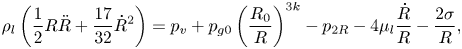 \begin{equation} \rho_l \left(\frac{1}{2} R\ddot{R} + \frac{17}{32}\dot{R}^2 \right) = p_v + p_{g0}\left(\frac{R_0}{R}\right)^{3k} - p_{2R} - 4\mu_l \frac{\dot{R}}{R} - \frac{2\sigma}{R}, \end{equation}
where  $R$ is the radius of the bubble with
  $\dot {R}$ and
  $\ddot {R}$ denoting its first and second temporal derivatives, respectively. The summation of the first two terms on the right-hand side is the bubble pressure, where
  $p_v$ is the vapour pressure and
  $p_{g0}({R_0}/{R})^{3k}$ is the dissolved gas pressure, with
  $p_{g0}$ and
  $R_0$ representing the initial equilibrium gas pressure and radius, respectively. The exponent,
  $k$, is set to 1 if the bubble content behaves isothermally and to
  $\gamma$ (gas polytropic constant) if the radius of the bubble varies adiabatically. Here,
  $p_{2R}$ is the surface-average pressure of the mixture over a concentric sphere with radius
  $2R$, which represents the local pressure around the bubble. To obtain the local pressure, other radial distances (e.g.
  $5R$) could also be used with similar accuracy. In such a case, one only needs to modify the constant coefficients on the left-hand side of the equation accordingly. Here, we assumed that a distance of
  $2R$ from the centre of the bubble can give a more accurate representation of the bubble local pressure when it is surrounded by other Lagrangian bubbles. Finally, the last two terms represent the viscous stress and surface tension stress on the interface, with
  $\sigma$ denoting the surface tension coefficient. Equation (3.21) can be conveniently implemented in different control volume-based solution algorithms.
The time-step adaptive second-order Rosenbrock method is implemented to solve the Rayleigh–Plesset equation numerically (see e.g. Shampine & Reichelt Reference Shampine and Reichelt1997 for a description of this approach). In the solution algorithm, all of the equation parameters should be specified. The surrounding fluid properties ( $\sigma$,
  $\mu$,
  $\gamma$ and
  $\rho$) are either constant values or surface-average interpolated at
  $5R$, as explained in the previous section. Additionally, the vapour pressure,
  $p_v$, is considered as the liquid–vapour saturation pressure at the flow temperature. Then, the only unknown term is the dissolved gas pressure, which is a function of the initial (or reference) radius,
  $R_0$, and gas pressure,
  $p_{g0}$, of the bubble. These parameters should be specified when a bubble is injected. For the Lagrangian solver, where new cavity structures are introduced as (parcels of) bubbles, at the injection time, a bubble is assumed to originate from a nucleus, which has been in an equilibrium condition far away from the cavitation zone, and it has been transformed by the flow and has grown in size owing to the pressure drop. In the equilibrium condition, the original form of the Rayleigh–Plesset equation can be simplified and leads to the following relation between the initial gas pressure and bubble radius:
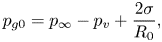 \begin{equation} p_{g0} = p_{\infty} - p_v + \frac{2\sigma}{R_0}, \end{equation}
where  $p_{\infty }$ is the far-field pressure, assumed to be 101 325 Pa. In this study, it is assumed that the radius of the assumed nuclei is 1
  $\mathrm {\mu }$m, which corresponds to
  $p_{g0} = 242$ kPa. However, it is possible in the solver to adjust these parameters based on the experimental data of water quality, if available. Additionally, in the hybrid model, when an Eulerian cavity is transformed to a Lagrangian bubble, initial values of
  $\dot {R}$ and
  $\ddot {R}$ are obtained based on the volume variation rate of the old Eulerian vapour, as will be described later. It was shown previously that (3.21) can adequately describe the collapse of a single bubble as well as a cluster of bubbles with random distribution and significant bubble interactions over a wall compared with the thermodynamic equilibrium model of Schmidt et al. (Reference Schmidt, Mihatsch, Thalhamer and Adams2011) as a reference solution (Ghahramani et al. Reference Ghahramani, Arabnejad and Bensow2019). It was also shown that the localized Rayleigh–Plesset equation provides a considerably more accurate estimation of the bubble collapse rate compared with the original equation with correction terms suggested by Hsiao et al. (Reference Hsiao, Ma and Chahine2017) and Giannadakis et al. (Reference Giannadakis, Gavaises and Arcoumanis2008). Further comparison with other earlier models is given in Appendix A.
3.2.4. Bubble–bubble collision
For the four-way coupling, the method for how bubble–bubble collisions are handled is a critical issue. There are two fundamental parts to the calculation of bubble collisions, the incidence of collisions and the outcome of collisions. The incidence of collisions is predicted using a deterministic algorithm similar to the work of Breuer & Alletto (Reference Breuer and Alletto2012) and only binary collisions are considered here. We first explain the algorithm for colliding bubbles and later this is extended for parcel collisions. To find the collision possibility between each bubble and other bubbles, instead of having a loop over all of the other bubbles, which is computationally expensive, we use a more efficient method and detect the bubble–bubble collision by a faster algorithm based on the ‘cell occupancy’ concept. The cell occupancy concept and the detection of possible collisions between the bubbles close to each other are described in detail in Appendix C. Using the cell occupancy property, it is possible to detect the collisions between the bubbles that are located at two sides of a processor boundary in a parallel computation, while in the previous approach, in which one needs to loop over all bubbles, it can be sophisticated and computationally expensive to send Lagrangian bubble information to a neighbouring processor.
After a collision, a pair of bubbles may coalesce to form a larger bubble or they may bounce back from each other, and this is specified based on the relative velocity and the interaction time of the bubbles. It is known that there is a limited time available for bubble–bubble interactions, and when two bubbles approach each other, a liquid film is trapped between them, which tends to resist any further movement that could bring the bubbles closer (Chesters Reference Chesters1991). If the interaction time is long enough that the liquid film can drain to a sufficiently small thickness and rupture, the bubbles may coalesce, otherwise they bounce back from each other. The outcome of the collision is therefore assumed to be a function of two time scales, the interaction time of the bubbles,  $t_i$, and the liquid film drainage time,
  $t_d$. According to Kamp et al. (Reference Kamp, Chesters, Colin and Fabre2001), these time scales are given by
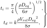 \begin{equation} \left. \begin{gathered} t_i = \frac{\pi}{4}{\left(\frac{\rho {D_{eq}}^3}{6 \sigma}\right)}^{1/2},\\ t_d = k\frac{\rho V_{rel}{D_{eq}}^2}{8 \sigma}, \end{gathered}\right\} \end{equation}
where,  $V_{rel}$ is the relative velocity between the two bubbles in the normal direction, and
  $D_{eq} = {4R_1R_2}/{(R_1+R_2)}$ is the equivalent diameter of the bubbles with radii
  $R_1$ and
  $R_2$. Additionally,
  $k$ is a correction factor which accounts for various approximations made in deriving the expressions for
  $t_i$ and
  $t_d$, and is set to 2.5 (Kamp et al. Reference Kamp, Chesters, Colin and Fabre2001). The theoretical coalescence probability for a head-on collision is
  $P_{coal} = 0$ if
  $t_i < t_d$ and
  $P_{coal} = 1$ if
  $t_i \geq t_d$. However, to account for the the fact that the collision may not be frontal, the coalescence probability is expressed as
 \begin{equation} P_{\mathit{coal}} = \textrm{e}^{{-}t_d/t_i}. \end{equation}
Then a random number is sampled from a uniform distribution function. If this number is larger than the coalescence probability, then the bubbles are assumed to bounce back after collision; otherwise, they are considered to coalesce. For the first scenario, the normal velocities of the bubbles after collision are calculated as
 \begin{equation} \left.\begin{gathered} u^+_{1n} = \frac{m_1 u^-_{1n} + m_2 u^-_{2n} - \epsilon m_2 (u^-_{1n} - u^-_{2n})}{m_1 + m_2},\\ u^+_{2n} = \frac{m_1 u^-_{1n} + m_2 u^-_{2n} + \epsilon m_1 (u^-_{1n} - u^-_{2n})}{m_1 + m_2}, \end{gathered}\right\} \end{equation}
where  $m_1$ and
  $m_2$ denote the mass of the bubbles,
  $u^-_{1n}$ and
  $u^-_{2n}$ are the corresponding normal velocities before collision (Appendix C), and
  $\epsilon$ is the restitution coefficient, which is set to 0.8 following Vallier (Reference Vallier2013). Here, it is assumed that the tangential velocity of the bubble does not change, which implies no friction between the colliding pair. If the bubbles coalesce after collision, then we need to estimate the properties of the new bubble. Following the work of Ilinskii et al. (Reference Ilinskii, Hamilton, Zabolotskaya and Meegan2006), this process is assumed to satisfy the following conservation relations:
 $$\begin{gather} V_1 + V_2 = V_3, \end{gather}$$
 $$\begin{gather}\dot{V}_1 + \dot{V}_2 =\dot{V}_3, \end{gather}$$
 $$\begin{gather}p_{B1} V_1 + p_{B2} V_2 = p_{B3}V_3, \end{gather}$$
 $$\begin{gather}\boldsymbol{x}_1 V_1 + \boldsymbol{x}_2 V_2 = \boldsymbol{x}_3 V_3, \end{gather}$$
 $$\begin{gather}\boldsymbol{u}_1 V_1 + \boldsymbol{u}_2 V_2 = \boldsymbol{u}_3 V_3, \end{gather}$$
where index 3 identifies the properties of the third bubble and  $V_i$ is the volume of the bubble, whose temporal variation rate is represented by
  $\dot {V}_i = 4\pi R^2_i \dot {R}_i$. Equations (3.26) and (3.27) conserve the vapour volume and kinetic energy, respectively. From these equations,
  $R_3$ and
  $\dot {R}_3$ are obtained. Equation (3.28) conserves the internal energy of the vapour inside the bubble. From this relation, the new bubble pressure,
  $p_{B3}$, is calculated, which in turn is used to estimate the dissolved gas pressure (
 $p_{g3}$), while
  $p_v$ is constant. Finally, (3.29) and (3.30) maintain a constant centre of mass and momentum, respectively, and, from them, we estimate the centre (
 $\boldsymbol {x}_3$) and velocity (
 $\boldsymbol {u}_3$) vectors of the new bubble.
As stated earlier, (3.23)–(3.30) describe the interactions between a pair of bubbles. For two bubbles, a collision occurs if the bubbles pass within the collision locus, a circle of the collision cross-section. For bubble parcels, we assume that the collision cylinder formed by the displacement and collision cross-section has a larger diameter. To take into account this larger collision locus, we assign an equivalent radius to each bubble group that is represented by a parcel. The equivalent radius is simply given as
 \begin{equation} R_{\mathit{eqv}, i} = {\left(\frac{3}{4\pi}V_{\mathit{tot},i}\right)}^{{1}/{3}} = {n_i}^{{1}/{3}}R_i, \end{equation}
where  $V_{\mathit {tot},i}$ and
  $n_i$ are the total volume vapour and number of bubbles that are represented by a specific parcel
  $i$. Hence, the equivalent diameter of the bubble pair in (3.23) should be calculated based on the equivalent radii of the parcels (i.e.
  $D_{eq} = {4R_{\mathit {eqv},1}R_{\mathit {eqv},2}}/({R_{\mathit {eqv},1}+R_{\mathit {eqv},2}})$). It should be noticed that the properties of each parcel (
 $R_i, \boldsymbol {x}_i, \boldsymbol {u}_i, m_i$, etc) are the same as the properties of the other bubbles that the parcel represents and the equivalent radii in the equations above are used to take into account the larger collision locus and hence collision probability between bubble groups, assuming that during the collision process each bubble group can be approximated by a larger bubble that has a similar vapour volume. If the parcels do not coalesce after collision, then (3.25) is used to update the normal velocities. However, because the total momentum of the bubble group should be considered in the collision, in this equation, the bubble mass (
 $m_i$) should be replaced by the total vapour mass (i.e.,
  $m_{\mathit {tot},i} = n_i m_i$). Additionally, if the parcels coalesce, in the conservation relations (3.26)–(3.30), the bubble volume and its temporal rate should be replaced by the corresponding values of the bubble group, i.e.
  $V_{\mathit {tot}, i}$ and
  $\dot {V}_{\mathit {tot},i}$.
3.2.5. Bubble break-up
The non-uniform pressure distribution and hydrodynamic forces in the surrounding fluid cause bubble deformation, which can lead to break-up. The break-up process can have different mechanisms regarding the governing physical process. The main mechanisms that have been studied extensively in the literature are: turbulent fluctuation and collision; viscous shear stress; shearing-off process; and interfacial instability (Lau et al. Reference Lau, Bai, Deen and Kuipers2014). From these mechanisms, bubble break-up because of turbulent fluctuation along the surface or by collision with eddies have been investigated most extensively. Giannadakis et al. (Reference Giannadakis, Gavaises and Arcoumanis2008) included break-up arising from both the turbulence and hydrodynamic forces (caused by the velocity difference between a bubble and surrounding fluid) in their Lagrangian cavitation model and concluded that most bubbles break because of turbulent break-up. Lau et al. (Reference Lau, Bai, Deen and Kuipers2014) also found the turbulent fluctuation mechanism to be the dominant break-up mechanism in a turbulent bubble column.
Regarding the break-up criterion for a bubble, four different criteria have been reported in the literature. The associated critical values involve bubble turbulent kinetic energy, the surrounding velocity fluctuation, turbulent kinetic energy of the impacting eddy and the inertial force of the eddy. However, Lau et al. (Reference Lau, Bai, Deen and Kuipers2014) showed that various reported models can be written in terms of a critical Weber number,  $We$. The
  $We$ can be regarded as a dimensionless ratio between the inertial force (which causes deformation) and the surface tension (which tends to restore the bubble sphericity). For turbulent flow around a bubble,
  $We$ can be defined as
 \begin{equation} We = \frac{\rho \overline{( u'_i u'_i )_{d_p}} d_p}{\sigma}, \end{equation}
where  $\overline {( u'_i u'_i )_{d_p}}$ is the mean square velocity difference over a distance equal to the diameter of the bubble. Because the deforming fluctuations are assumed to be of the same size as the diameter
  $d_p$ of the parent bubble, the characteristic length in (3.32) is the diameter of the bubble and the velocity difference is estimated over the same distance. The criterion for bubble break-up is usually defined as a critical value for
  $We$. For instance, Giannadakis et al. (Reference Giannadakis, Gavaises and Arcoumanis2008) used a critical value of 12, which is similar to what Lau et al. (Reference Lau, Bai, Deen and Kuipers2014) have derived for spherical bubbles.
Similar to most break-up models reported in the literature, we assume a binary break-up in the current study. The size of daughter bubbles is determined by the break-up volume fraction,  $f_{bv}$. Here,
  $f_{bv}$ is a random variable and can be either based on empirical observations or acquired from a statistical distribution. Various daughter bubble size distributions (uniform, normal, U-shape and M-shape) have been presented in the literature. In a recent study, Hoppe & Breuer (Reference Hoppe and Breuer2020) derived a relation for the critical
  $We$ based on the break-up volume fraction, given as
 \begin{equation} We_{\textit{crit}} = 12 \frac{d_p}{d_s} = 12 f^{-{1}/{3}}_{bv}, \end{equation}
where  $d_s$ denotes the diameter of the small daughter bubble. The ratio
  $f^{-{1}/{3}}_{bv}$ has a minimum value of
  $0.5^{-{1}/{3}} = 1.26$ for a break-up into two equally-sized daughter bubbles. In this case, the critical
  $We$ has a minimum value of 15.12, which is the closest one to the corresponding value mentioned above. Other daughter size distributions would correspond to larger values of critical
  $We$, which means a larger turbulent kinetic energy to break the deformed bubbles. In this study, the bubbles are assumed to break-up into equally-sized daughter bubbles and the
  $We$ is considered to be 15.12. This makes the implementation simpler as well, as there is no need to define a new parcel, but only the number of bubbles that the parcel is representing is doubled.
To calculate the properties of the daughter bubbles, it is assumed that the break-up process follows similar conservation relations that were used for the description of the bubble coalescence process. It is obvious that during break-up of each bubble into two bubbles with  ${d_p}/{d_s} = 1.26$, the vapour volume is conserved and the number of bubbles represented by each parcel (
 $n_i$) is doubled. Having
  $R_i$ and
  $n_i$, the growth rate of daughter bubbles can be obtained from the conservation of kinetic energy (identical to (3.27)). Then, the internal energy conservation relation (similar to (3.28)) is used to calculate the dissolved gas pressure of the bubble. Because the daughter parcels are equal and the vapour volume is conserved during this process, the position and velocity vectors of the parcel do not vary during the break-up process.
The Lagrangian model is a four-way coupling model as both bubble–flow interactions and bubble–bubble interactions are considered. Additionally, the discretizations and solution algorithm for the Eulerian equations of this model are exactly the same as those of the homogeneous mixture model. At each time step, the continuity and Navier–Stokes equations ((3.1) and (3.2)) are solved first and the updated pressure and velocity field are used to solve the Lagrangian transport equation (3.15), bubble dynamics equation (3.21), and bubble interactions with each other and with flow boundaries. The updated bubble size and distribution are then used to update the volume fraction value ( $\beta$) to obtain the new mixture properties for the next time step. The Lagrangian model performance was verified earlier against benchmark test cases for the collapse of a single bubble and a cluster of bubbles (Ghahramani et al. Reference Ghahramani, Arabnejad and Bensow2019).
3.3. The multi-scale hybrid model
In the hybrid model, the large vapour structures are modelled through the Eulerian mixture approach and the small-scale structures are represented as discrete bubbles. The governing equations of the continuous flow field are similar to the previous models (i.e. (3.2)–(3.7)) and the main difference is in the tracking of the cavity structures. Here, the cavities are categorized as Eulerian structures and Lagrangian bubbles to be tracked in the corresponding framework.
As mentioned in § 2, the categorization of the structures into Lagrangian and Eulerian groups is done based on the size of each cavity relative to the local grid size of the discretized domain. If a cavity is large enough to be resolved by a sufficient number of computational cells, then it is tracked in the Eulerian framework, otherwise it is treated as parcels of Lagrangian bubbles. Furthermore, as the volume of each cavity can change in the flow, at each time step, the small Eulerian structures or large Lagrangian cavities may be transformed from one framework to the other. In the previous sections, the cavity volume fraction is specified by either the  $\alpha$ or
  $\beta$ parameters, but here, the governing equations should be revised to consider both Lagrangian bubbles (
 $\beta$) and Eulerian cavities (
 $\alpha$) together in the solution algorithm. Furthermore, another algorithm needs to be defined for the transformation of Eulerian cavities to Lagrangian bubbles and vice versa. In the earlier study by Ghahramani et al. (Reference Ghahramani, Arabnejad and Bensow2018), this algorithm and the necessary revisions in the governing equations were explained in detail, and in the following paragraphs, a summary of them with some new details of the transition process are presented.
3.3.1. Eulerian–Lagrangian transition
In the current transition algorithm, cavities are transformed directly from one framework to the other. At each time step, small Eulerian cavity structures that are not resolved by a sufficient number of computational cells are transformed to Lagrangian bubbles. Eulerian cavity structures are recognized in the flow domain by the hosting cells liquid volume fraction, which is less than 1. Thus, to remove an Eulerian structure, the corresponding liquid volume fraction of the respective cells ( $\alpha$) needs to be set equal to 1. This transition is shown schematically in figure 3 for a simple 2-D grid. The grid cells that have Eulerian cavities are coloured blue with
  $\alpha < 1$. Two of the cavities are resolved only by four cells and they are replaced by Lagrangian bubbles. Additionally, if a Lagrangian cavity later becomes large enough, it is transformed back to a Eulerian structure by deleting the corresponding bubbles and setting a new
  $\alpha$ value in the occupied cells. Furthermore, if each Lagrangian bubble approaches a large Eulerian structure, it is transformed to the Eulerian framework and becomes a part of that large cavity. As explained by Ghahramani et al. (Reference Ghahramani, Arabnejad and Bensow2018), when bubbles replace a cavity cloud by setting the
  $\alpha$ value to 1 without considering the effect of new bubbles in the mixture properties (as described in § 3.2.1), the sudden change in the
  $\alpha$ value will cause a jump in the values of the mixture properties,
  $\rho _m$ and
  $\mu _m$, (based on (3.3) and (3.5)) as well as the mass transfer source term (3.7). Such significant changes can cause spurious numerical pressure pulses, which may have considerable unrealistic effects on the flow field and the resulting erosion/noise prediction. The same scenario can occur when a Lagrangian cavity is transferred to an Eulerian cloud (see (3.11a,b)). Therefore, the governing equations of the continuous flow should be written based on a new parameter that is conserved during the transition process. As explained in an earlier study (Ghahramani et al. Reference Ghahramani, Arabnejad and Bensow2018), the improved relations for mixture properties and mass transfer rate are given as
 \begin{gather} \left.\begin{gathered} \rho_m = \alpha\beta \rho_l + (1-\alpha\beta) \rho_v ,\\ \mu_m = \alpha\beta \mu_l + (1-\alpha\beta) \mu_v, \end{gathered}\right\} \end{gather}
 \begin{gather} \left.\begin{gathered} \dot{m}_c = C_c \alpha\beta(1 - \alpha\beta) \frac{3 \rho_l \rho_v}{\rho_m R_B}\sqrt{\frac{2}{3\rho_l |p - p_{\mathit{threshold}}|}} \max(p - p_{\mathit{threshold}}, 0),\\ \dot{m}_v = C_v \alpha\beta(1 + \alpha_{\mathit{Nuc}} - \alpha\beta) \frac{3 \rho_l \rho_v}{\rho_m R_B}\sqrt{\frac{2}{3\rho_l |p - p_{\mathit{threshold}}|}} \min(p - p_{\mathit{threshold}}, 0). \end{gathered}\right\} \end{gather}
Here, the earlier  $\alpha$ (or
  $\beta$) terms are replaced by their product
  $\alpha \beta$. It is obvious that in cells containing an Eulerian cavity,
  $\alpha$ is less 1, while it is equal to 1 everywhere else. Similarly, in cells containing bubbles,
  $\beta$ is less than 1, while it is equal to 1 everywhere else. During the Eulerian to Lagrangian transition, the new value of
  $\beta$ in the cavity hosting cells is the same as the old value of
  $\alpha$ and vice versa. Therefore, both
  $\alpha$ and
  $\beta$ have similar sudden changes while their product
  $\alpha \beta$ does not change during the Eulerian–Lagrangian transition. In the cells containing bubbles, where
  $\alpha = 1$,
  $\alpha \beta$ has the same value as
  $\beta$ and in Eulerian cavity zones, where
  $\beta = 1$,
  $\alpha \beta$ is equal to
  $\alpha$. It is important to note that in each computational cell, the vapour structure should be represented in either a Eulerian or Lagrangian framework. Therefore, in the cells containing bubbles, the generation of the Eulerian cavities should be avoided by revising the
  $\alpha$ transport equation source term as (Ghahramani et al. Reference Ghahramani, Arabnejad and Bensow2018)
 \begin{equation} \frac{\partial \alpha}{\partial t} + \frac{\partial (\alpha u_i)}{\partial x_i } = \frac{\dot{m}}{\rho_l}*\textrm{pos}(\beta - 1). \end{equation}
The pos( $x$) function returns 1 when
  $x \geq 0$, otherwise it returns 0. When there is a bubble in a cell,
  $\beta$ is less than 1; therefore, the
  $\textrm {pos}(\beta - 1)$ equals zero and no cavity is generated in the cell. To the best of the authors’ knowledge, the revision of governing equations ((3.34)–(3.36)) is missing in the earlier hybrid models of this type. An exception is the recent study by Peters & El Moctar (Reference Peters and El Moctar2020), in which the Lagrangian bubbles contribution to the mixture properties is taken into account. Here, we have developed the modelling one step further by considering the bubble effects in the mass transfer rate and
  $\alpha$ transport equations (Ghahramani et al. Reference Ghahramani, Arabnejad and Bensow2018).

Figure 3. Transition of small Eulerian cavities to Lagrangian bubbles.
Another important point in the transition process is the specification of new bubble properties. The small Eulerian cavities, which are transformed to the Lagrangian framework, are usually sparse clouds with a low vapour concentration. Therefore, it is not realistic to replace the whole structure with one single bubble of pure vapour but one should use a cloud of smaller bubbles. The small bubbles can have different distributions in size and position, and to decrease the computational expenses, it is suggested to keep the number of bubbles as low as possible. Furthermore, to ensure local conservation of vapour volume in each computational cell, the vapour content of each individual cell is replaced by relative individual parcels whose diameter is less than the minimum edge of the cell (Ghahramani et al. Reference Ghahramani, Arabnejad and Bensow2018), figure 3. Then the vapour volume of each cell is replaced by at least one parcel and the number of bubbles for that parcel is defined based on the vapour volume conservation. If the size of the new parcel ( $\leq$ minimum cell edge) is larger than a realistic physical value, it breaks-up into smaller parcels following the described break-up model. When the bubble radius and the number of bubbles for each parcel are determined, other Lagrangian properties can be specified based on the conservation relations and equilibrium equations. The growth rate of the bubble,
  $\dot {R}$, and its temporal rate,
  $\ddot {R}$, are obtained from the corresponding values for the Eulerian cavity as
 \begin{equation} \left.\begin{gathered} \dot{R}_i = \frac{\dot{V}_{v,j}}{n_i q_j 4\pi R^2_i},\\ \ddot{R}_i = \frac{\ddot{V}_{v,j} - n_i q_j 8\pi R_i \dot{R}^2_i}{n_i q_j 4\pi R^2_i}, \end{gathered}\right\} \end{equation}
where  $q_j$ is the number of parcels in cell
  $j$,
$j$,  $\dot {V}_{v,j}$ denotes the growth rate of Eulerian vapour volume in the cell and
  $\ddot {V}_{v,j}$ is its temporal rate. A correct initialization of
  $\dot {R}$ and
  $\ddot {R}$ is an important point, which is not taken into consideration in the earlier hybrid cavitation models. This is depicted in figure 4 for the collapse of a single isolated bubble exposed to the atmospheric pressure at infinity. Here, the effects of viscosity, dissolved gas and surface tension are ignored. This problem is known as Rayleigh bubble collapse and can be solved analytically up to the collapse time. The liquid is assumed to be incompressible and because the dissolved gas effect is ignored, the bubble has a full collapse. In an earlier study (Ghahramani et al. Reference Ghahramani, Arabnejad and Bensow2019), it was shown that both Eulerian mixture and Lagrangian bubble models can accurately predict the temporal variation of the bubble radius. In figure 4, the hybrid model result is compared with the exact analytical solution. The horizontal axis is the time, non-dimensionalized by the final collapse time, and the vertical axis is the dimensionless radius. In the simulation, the
  $0.4$ mm bubble is initially modelled using the mixture model, and when
  $R/R_0 = 0.6$, the cavity is transformed to the Lagrangian framework. We can see that using (3.37), the numerical result follows the theoretical pattern, while the collapse time will have a significant delay if the initial value of
  $\dot {R}$ is set to 0.
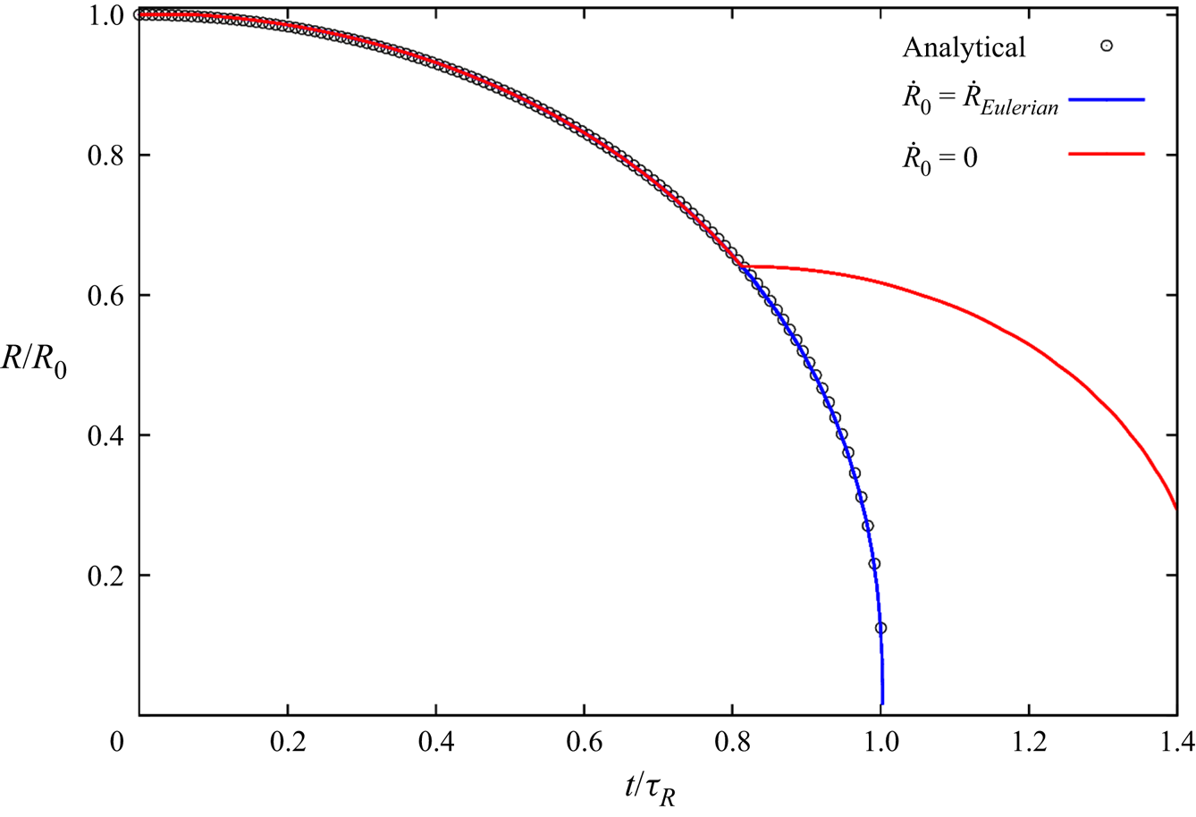
Figure 4. Effect of initial growth rate on the bubble collapse.
Regarding the initialization of the remaining parameters, the initial density and velocity of the parcel are set equal to the vapour density and cell velocity, respectively. Finally, the initial radius of the bubble,  $R_0$ is set to 1
  $\mathrm {\mu }$m and the corresponding initial dissolved gas pressure (
 $p_{g0}$) is estimated from (3.22), as stated earlier.
Algorithm 1 Eulerian to Lagrangian transition algorithm

Another point regarding the compatibility of the two frameworks is the mass transfer at the interface. In the derivation of the Rayleigh–Plesset equation, the mass transfer through the interface is neglected (Franc & Michel Reference Franc and Michel2006) and the bubble size varies based mainly on the difference between the bubble pressure and its surrounding pressure, as well as surface tension and viscosity effects. For the Eulerian model, there is a source term in the vapour transport equation (3.6), based on which the vapour volume and the mixture density varies. However, this source term is also mainly a function of the pressure difference. As stated previously, the finite mass transfer models, such as the applied Schnerr–Sauer model, can be interpreted as a simplified form of the Rayleigh–Plesset equation, in which the dissolved gas pressure, surface tension and viscous forces are neglected and the bubble inertia is simplified by neglecting the second temporal derivative of the bubble radius.
After explaining different aspects of the Eulerian to Lagrangian transition, the overall algorithm of this process can be summarized now. In the first step, all of the cavity structures in the flow domain are detected. Next, the number of computational cells that represent each structure are counted. To measure the size of an Eulerian cavity, the computational cells with  $\alpha \leq \alpha _{lim}$ are counted as vapour cells. If the number of cells is less than a threshold value, denoted as
  $N_{EL}$, it is decided that the relative structure is not represented by a sufficient number of grid cells. Then, for each cavity that is not well resolved, Algorithm 1 is followed. Because the liquid–vapour interface is diffuse in mixture modelling, in addition to the cell group with
  $\alpha \leq \alpha _{\textit {lim}}$, there are other neighbouring cells with
  $\alpha _{\textit {lim}} < \alpha < 1$. In the transition algorithm, the vapour content of these cells are also transferred to small Lagrangian bubbles.
Additionally, if a Lagrangian bubble collides with a large Eulerian cavity or it becomes large enough to be resolved by sufficient number of cells, it will be transformed to an Eulerian structure by deleting the bubble, while in the host cell,  $\beta$ is set to 1 and
  $\alpha = \beta _{\mathit {old}}$. In this study, the transition criterion is based on a threshold number of grid cells. In the solver implementation, the user can set two parameters,
  $N_{EL}$ and
  $N_{LE}$, which are the threshold numbers of cells, based on which an Eulerian structure is transformed to a group of Lagrangian bubbles and vice versa, respectively. Such a criterion can be dependent on the grid resolution as the numbers should be specified based on the sufficiency of a grid in resolving an Eulerian cavity. In the following section, the effect of these numbers in the solver performance is investigated. Applying more suitable criteria for the transition algorithm can be the subject of a future study.
As mentioned earlier, the hybrid solver is developed based on the coupling of the presented Lagrangian model with the the solver interPhaseChangeFoam in OpenFOAM. In this solver, the pressure (continuity) and velocity (momentum) equations are coupled using a PIMPLE algorithm (OpenFoam 2018). This algorithm is a merge of the SIMPLE (Patankar & Spalding Reference Patankar and Spalding1983) and PISO algorithms, where the PISO loop is complemented by an outer iteration loop, see e.g. Barton (Reference Barton1998) for different ways to merge the PISO and SIMPLE procedures. In the current study, at each time step, four outer SIMPLE loops are performed, and in each SIMPLE loop, four PISO pressure-correction loops are performed. The final solution algorithm of the hybrid solver is depicted in figure 5.
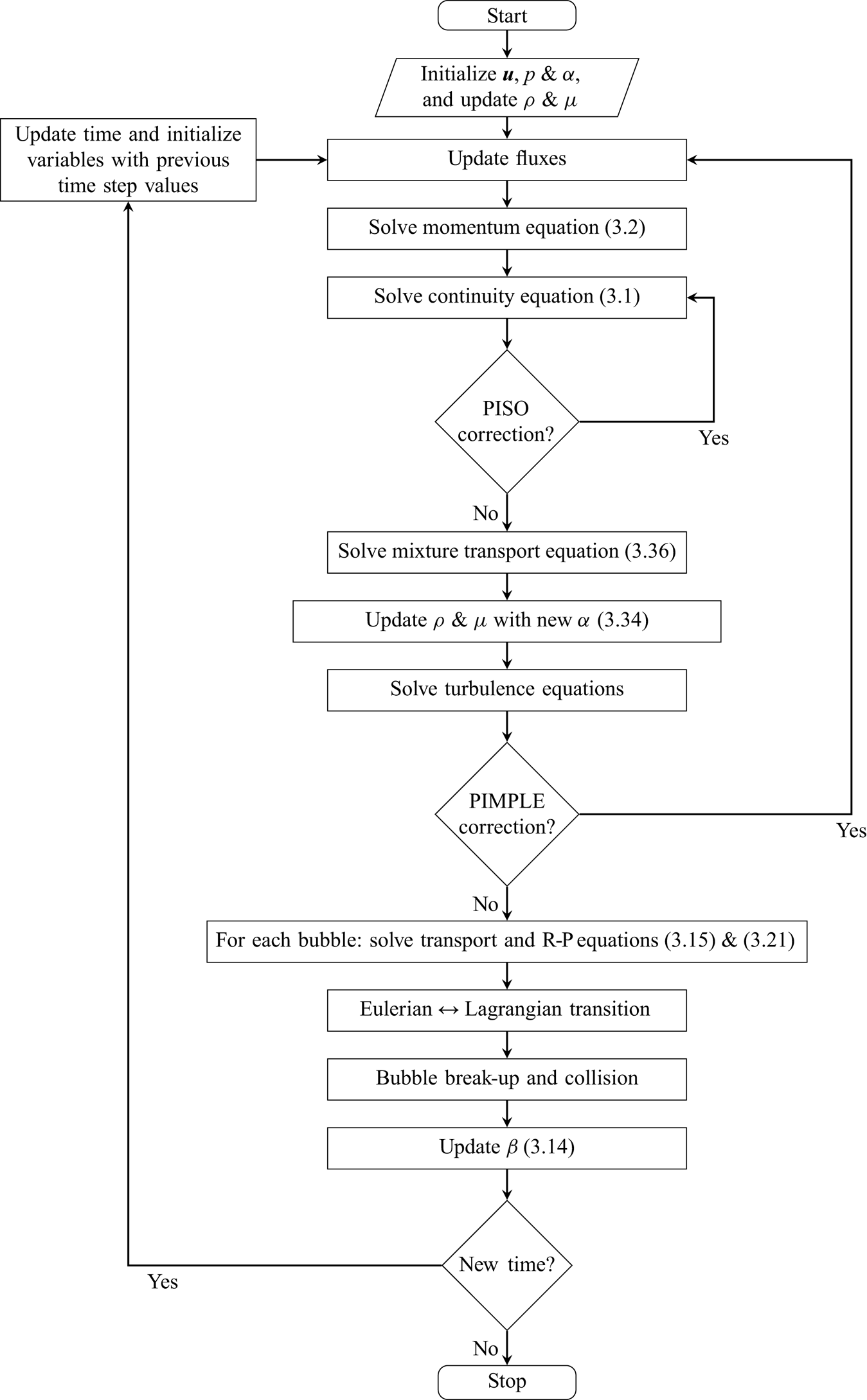
Figure 5. Hybrid solver algorithm.
4. Cavitating flow around a sharp-edge bluff body
The multi-scale problem is a periodic cavitating flow around a bluff body. We use this case to both validate the numerical model and investigate some of the flow characteristics at different scales of a cavitation problem. Based on our experience and earlier studies in the literature, this set-up can generate various cavity structures with different length scales that have aggressive collapses, which are highly erosive at low cavitation numbers. For example, Escaler, Avellan & Egusquiza (Reference Escaler, Avellan and Egusquiza2001) compared four different bluff bodies and found the flat-front semi-circular cylinder to be an adequate geometry for generating reproducible pitting on the specimen within a short period of time. However, a reliable numerical study of the cavitating flow around this geometry, which can provide detailed information of the flow physics, has not been done yet. Additionally, as will be seen later, the cavitation development in this test case includes various structures with different length scales.
The bluff body is a flat-front semi-circular cylinder that is mounted on a surface in the throat of a convergent–divergent channel. The mounted cylinder and a simple sketch of the test section are depicted in figure 6. The channel has a rectangular cross-section with dimensions of  $74\times 54$ mm
 $^{2}$ which contracts to a section of
  $25\times 54$ mm
 $^{2}$ through a curved profile upper wall and a simple
  $45\,^\circ$ slope on the lower wall, while the channel width is constant everywhere. The bluff body is put at the end of the lower slope and after that, there is a flat plate with dimensions of
  $106\times 54$ mm
 $^{2}$. The flat side of the cylinder is facing upstream and at the attachment of the flat plate and the sloped wall, there is a small backward facing step with a height of
  $0.5$ mm. The cylinder has a diameter of
  $5$ mm and a length of
  $9.65$ mm. The cavitation number is defined as
 \begin{equation} \sigma = \frac{p_d - p_v}{\frac{1}{2} \rho u_{th}^2}, \end{equation}
where  $p_d$ is the downstream pressure,
  $p_v$ is the vapour pressure and
  $u_{th}$ is the area-averaged velocity of the flow at the throat of the converging–diverging section without the cylinder. The downstream pressure is measured at a distance of
  $500.5$ mm after the bluff body. The pressure probe location can be seen in figure 6(b). The experimental data have been captured using high-speed imaging in an earlier study (Ghahramani et al. Reference Ghahramani, Jahangir, Neuhauser, Bourgeois, Poelma and Bensow2020) for a vast range of cavity patterns. Further details about the set-up as well as the experimental procedure can be found in the same paper. Here, we choose a periodic cavity pattern which corresponds to a cavitation number of
  $0.893$, volumetric flow rate of
  $0.0257$ m
 $^{3}$ s
 $^{-1}$ and downstream pressure of
  $164$ kPa. This case includes various structures at different length scales.
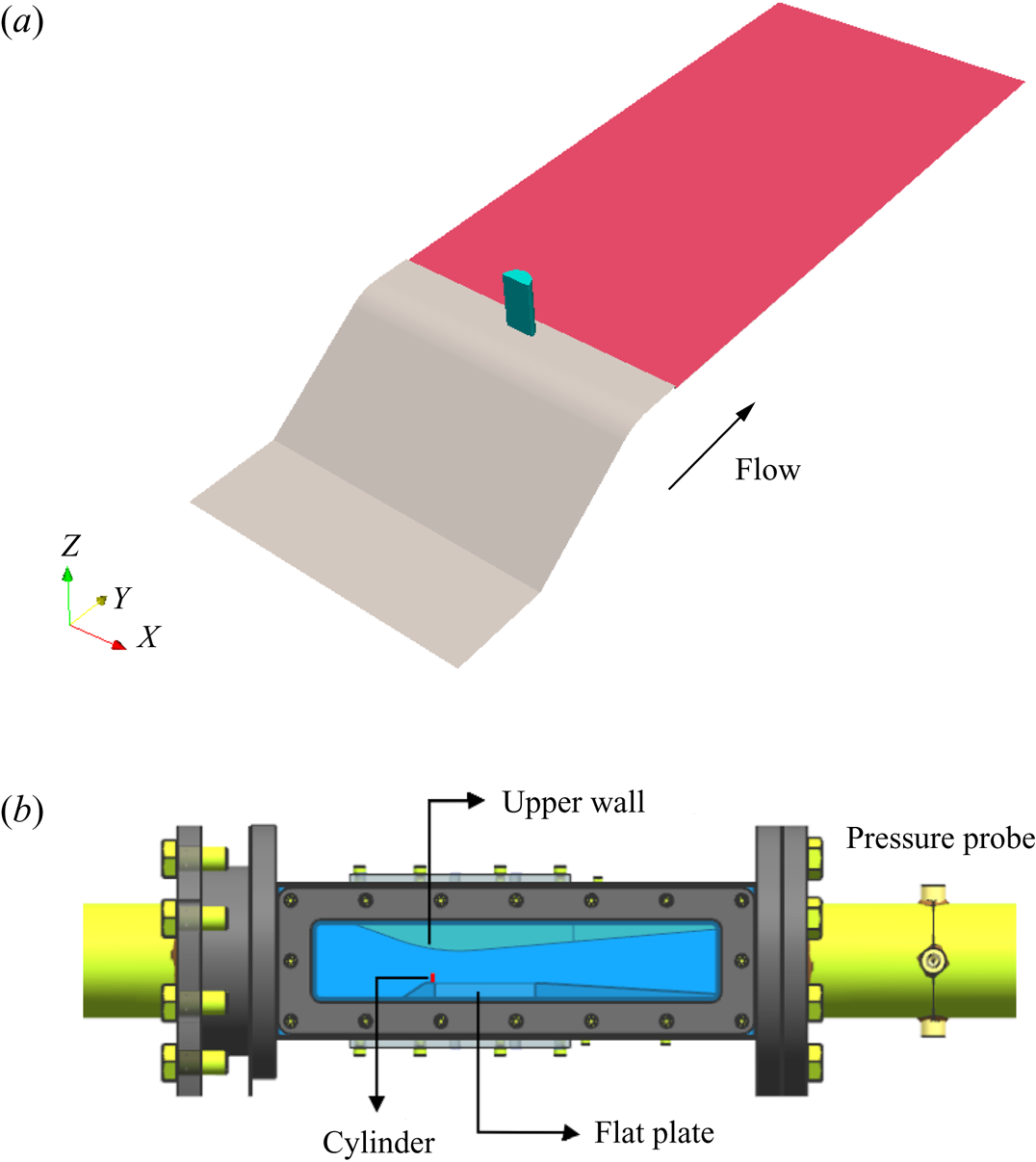
Figure 6. Test case: (a) lower wall and bluff body; (b) test section (dimensions not to scale). The images are taken from the paper by Ghahramani et al. (Reference Ghahramani, Jahangir, Neuhauser, Bourgeois, Poelma and Bensow2020).
4.1. Simulation set-up
The created numerical domain is depicted in figure 7, which includes the domain inlet and outlet boundaries, as well as the pressure probe location and the small cylinder in the converging–diverging section of the channel. To avoid the influence of the inlet and outlet boundaries on the flow field in the converging–diverging part of the channel and the measured pressure at the probe location, these boundaries are located sufficiently far from the test section. In the figure,  $w$ denotes the channel width normal to the plane, which is constant in the whole domain. At the inlet, a constant volume flow rate of
  $0.0257$ m
 $^{3}$ s
 $^{-1}$ is applied for the velocity field while the pressure gradient is set to zero. At the outlet, a constant pressure is set such that the probe pressure
  $p_d$ is equal to
  $164$ kPa, while a zero gradient condition is set for the velocity. These values correspond to test case 3 in the experimental work with a cavitation number of
  $0.893$ (Ghahramani et al. Reference Ghahramani, Jahangir, Neuhauser, Bourgeois, Poelma and Bensow2020). Furthermore, a no-slip condition is applied on all solid boundaries including the bluff body.
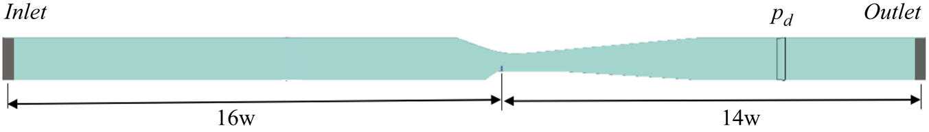
Figure 7. Computational domain;  $w$ denotes the channel width. The image is taken from the paper by Ghahramani et al. (Reference Ghahramani, Jahangir, Neuhauser, Bourgeois, Poelma and Bensow2020).
To discretize the flow domain, a structured mesh consisting of 4.8 million cells is created using ANSYS/ICEM. The top and side views of the generated grid are shown in figure 8 with zoomed views around the body and lower wall. The 0.5 mm height backward facing can be seen in the zoomed views. The mesh is non-uniform with finer cells around the cylinder and near the walls. If we consider the area from the start of the sloped wall to the end of the flat plate behind the cylinder as the critical area, 2.5 million cells of the generated grid are located in this zone. Additionally, the length of the wake flow behind the cylinder and in the axial direction (the flat-plate length) is discretized by approximately 150 grid nodes, while the number of nodes used for the cavity height and width are approximately 65 and 45, respectively.
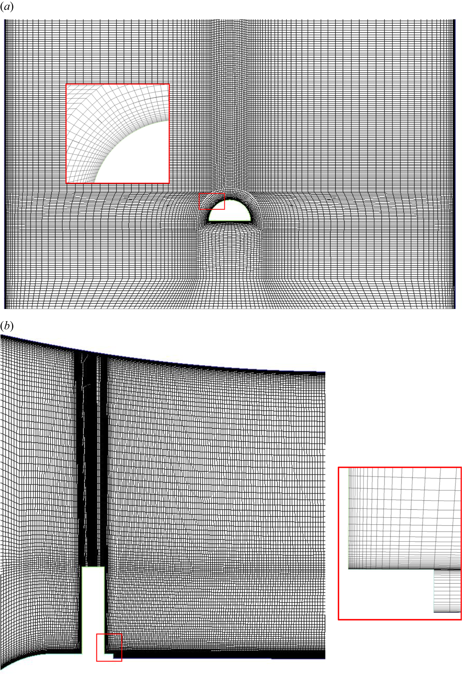
Figure 8. Domain discretization: (a) top view; (b) side view. The images are taken from the paper by Ghahramani et al. (Reference Ghahramani, Jahangir, Neuhauser, Bourgeois, Poelma and Bensow2020).
To study the influence of the grid resolution on the predicted results, in a previous study (Ghahramani et al. Reference Ghahramani, Jahangir, Neuhauser, Bourgeois, Poelma and Bensow2020), the cavitating flow (by the Eulerian model) was calculated using a finer grid with 10.8 million cells as well. From the predicted values for the pressure drop in the channel, as well as the drag coefficient on the bluff body, it was found that using a finer grid does not alter the averaged flow parameters significantly and therefore the 4.8 million cell grid is used in this study. In addition to the main grid results, the flow is simulated with a coarser grid to investigate the hybrid model performance with a lower grid resolution. The coarser grid is composed of 1.6 million cells with 0.6 million cells in the critical area.
Regarding the discretization of the governing equations, a second-order implicit time scheme is used for time discretization and the time step is set to  $1.5\times 10^{-7}$ s, which yields a maximum Courant number of
  $0.3$. As turbulence is modelled using the ILES approach, the momentum equation convection terms are discretized using a total variation diminishing limited linear interpolation scheme with a limiter value of 0.5. All of the gradients have been corrected to consider non-orthogonality of the computational cells. For the volume fraction transport equation, a first-order upwind scheme is employed, and to improve the coupling between the volume fraction equation and velocity–pressure equations, the transport equation of the liquid volume fraction is solved inside the PIMPLE loop (figure 5). A detailed explanation of the discretization of the Eulerian governing equations can be found in the work by Asnaghi (Reference Asnaghi2015).
4.2. Cavitation regime
We start by briefly describing the features of the cavitating flow around the bluff body using the experimental results. All of the experimental results that are shown below are from an earlier study (Ghahramani et al. Reference Ghahramani, Jahangir, Neuhauser, Bourgeois, Poelma and Bensow2020) and in all figures, the flow is from left to right. Additionally, in all of the time series of the flow that are illustrated in this paper,  $\Delta T = 4\times 10^{-5}$ s. The cavitation pattern of the described test case is shown in figure 9. After separation of the flow from the cylinder edges, different vortices are generated in the streamwise, spanwise and transverse directions. Here, by streamwise we mean the main flow direction, while spanwise is the direction along the cylinder span and normal to the flat plate behind it, and transverse is the other cross-stream direction normal to the spanwise direction. The low pressure vortices are first generated in the spanwise and transverse directions, and from their interactions with each other and the main flow, secondary streamwise vortices are created afterwards. The cavities have a cyclic pattern, which means that they shed periodically from the cylinder wake region.

Figure 9. Instantaneous cavity structures from an inclined-top view. (a–e) represent a time series. C31 and C32 represent two spanwise cavitating vortices. The images are taken from the paper by Ghahramani et al. (Reference Ghahramani, Jahangir, Neuhauser, Bourgeois, Poelma and Bensow2020).
In figure 9(a–e), a time series of cyclic cavity development is depicted. The streamwise and spanwise cavities are visible from the inclined-top view in this figure; however, the less cavitating transverse vortices are more detectable as large dots in the 2-D side view in figure 10 (e.g. cavities TC1 and TC2). At time  $T_0$, a spanwise cavitating vortex, C31, is created on the cylinder surface. As this vortex detaches from the cylinder, its vapour content increases and the cavity grows (
 $T_0 + 5\Delta T$). Meanwhile, a second larger spanwise cavity, C32, is seen downstream of C31. While the first cavity is developing behind the cylinder, the second one is shed from the body and its vapour content is decreasing, as shown in figure 9(c,d). Finally, at time
  $T_0+ 51\Delta T$, the second cavity is detaching in the form of a horseshoe vortex, while C31 is completely developed and has a similar shape as of the second cavity in the beginning of the time series (figure 9a). It should be mentioned that the revolving spanwise cavitating vortices are not always distinct from each other, and sometimes a spanwise cavity may grow and interact with a subsequent spanwise cavity as well as other vapour structures and evolve to a larger vapour pocket, similar to that in figure 9( f). Horseshoe vortices are not developed from spanwise cavities alone, but a combination of spanwise and transverse cavities that started at the top edge of the cylinder. The horseshoe vortices cannot last long as cavitating and they often lose most of their vapour content before reaching the half length of the flat plate; however, at specific times, a vortex may survive until approximately two-thirds of the plate length, as shown in figure 9( f). Sometimes a horseshoe vortex is not developed, but because of the interactions between cross-streamwise vortices with each other and the main flow, a streamwise vortex is created and stretched, which leads to streamwise cavities, as can be seen in figure 9( f) as well.
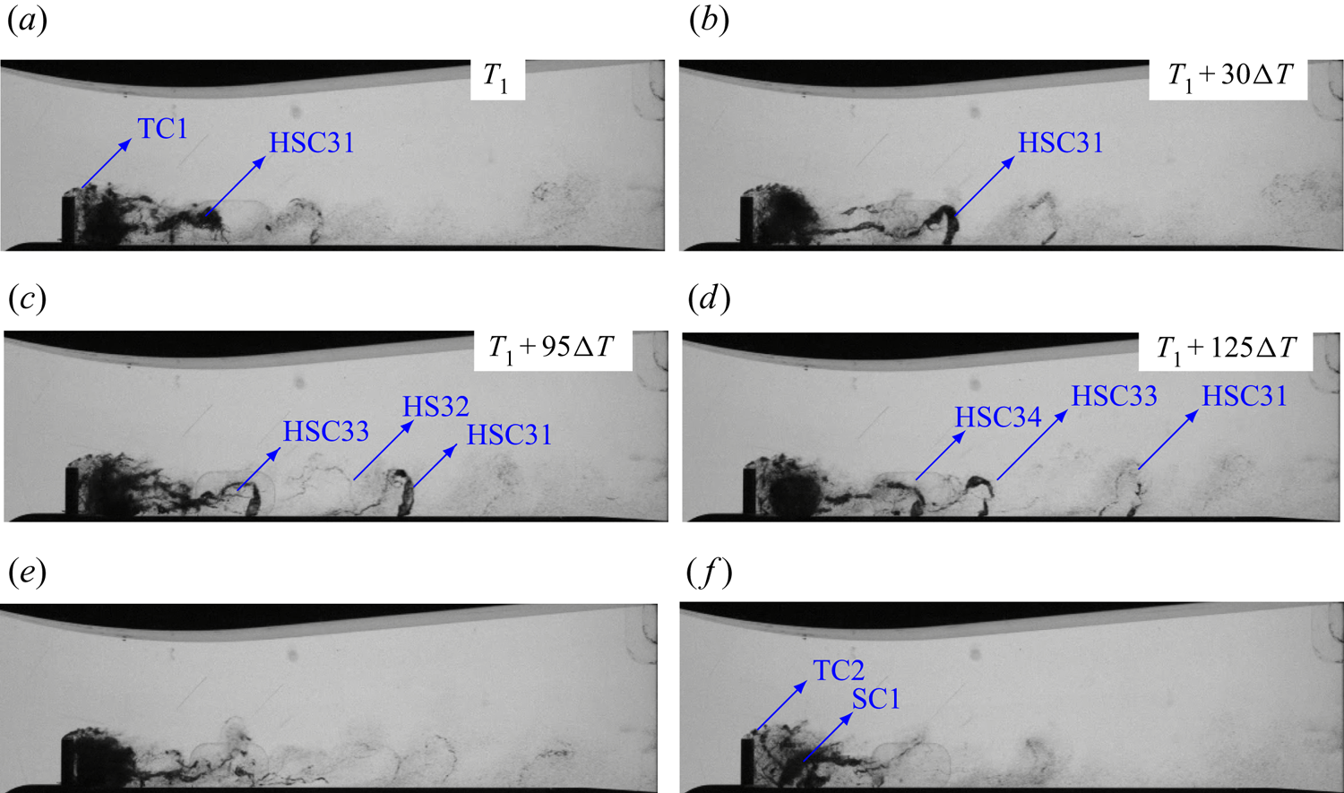
Figure 10. Instantaneous cavity structures from the side view. (a–d) represent a time series. TC, HSC and SC stand for transverse cavity, horseshoe cavity and streamwise cavity, respectively. The images are taken from the paper by Ghahramani et al. (Reference Ghahramani, Jahangir, Neuhauser, Bourgeois, Poelma and Bensow2020).
In figure 10, the cavity pattern is shown from the side view. Here, another time series of the flow is demonstrated in figure 10(a–d) to show the shedding of horseshoe vortices. We see that while the vortices HSC31, HSC33 and HSC34 are cavitating, the vortex HS32 is almost non-cavitating. It can be inferred from the time series that the streamwise and horseshoe vortices are not always cavitating and while a horseshoe vortex has a considerable vapour content (e.g. figure 10b), its subsequent vortex might be almost non-cavitating. The non-cavitating vortex is not as visible as the other structures; however, its presence can be further confirmed by the distance between HSC31 and HSC33, which is approximately twice the distance between HSC33 and HSC34. From figures 9 and 10, it can also be inferred that the near-wake transverse vortices are less cavitating compared with their spanwise correspondents. This can be seen from the lower vapour content in the core of the transverse vortices in the side-view images. Furthermore, from the side-view images, we can see the dispersed vapour bubbles and the horseshoe vortices with small vapour contents far downstream of the flow field. It is also worth mentioning that while at some instances, dense cavities with high vapour content can be seen behind the cylinder (e.g. figure 10e), there are other instances at which the near-wake cavities are fully or partially transparent, similar to what is shown in figure 10( f), and this reveals the very unsteady nature of the flow field around the bluff body.
4.3. Eulerian mixture model
In this section, the Eulerian mixture model performance (without any Lagrangian modelling of small scales) is investigated. Figure 11 shows the obtained cavity pattern from the Eulerian model based on the liquid fraction iso-surfaces. Here, the light grey colour represents the iso-surface of  $\alpha = 0.9$, and the black colour represents the iso-surface of
  $\alpha = 0.5$. Comparing the iso-surfaces with the experimental results (figures 9 and 10), it is evident that the cavity volume is underestimated using the Eulerian model. The underestimation is so considerable that some of the main features, explained in the previous section, are not captured in the results. While the cavitation should start on the cylinder surface, in the numerical results, we see that the inception is postponed and small vapour structures appear at a distance from the body. To be more precise, while in experiment, the first spanwise cavitating vortices starts to cavitate from the sharp edges of the cylinder, here, the first spanwise cavities, which partially cavitate, appear after the backward step behind the cylinder. In fact, at most times, we see a no-cavity zone close to the cylinder.

Figure 11. Contours of liquid volume fractions of 0.9 (light grey) and 0.5 (black) obtained by the Eulerian mixture model. Panels (a–e) represent a time series. Panel ( f) shows an instance with more vapour volume. Here, EC1 and EC2 represent two spanwise cavitating vortices and ES1 is a streamwise cavitating vortex.
To further understand the model performance, figure 11 includes a time series of cavitation development. At time  $T_0$, we see a small (partially) cavitating spanwise vortex, EC1, in the wake area and immediately after the small backward step. At the same time, there is a streamwise caviting vortex at the end of the cavitation zone, ES1, and between these two, there is a second larger spanwise vortex, EC2. At time
  $T_0 + 5\Delta T$, the cavity EC1 moves downstream and the streamwise vortex has less vapour content. Just a few time steps later,
  $T_0 + 10\Delta T$, the cavity EC1 starts to collapse, which is in contrast to the real case where the spanwise cavity keeps growing (as shown in figure 9b,c). At this time, we see that the streamwise cavity has also partially collapsed. At a later time,
  $T_0 + 15\Delta T$, the cavity EC1 has almost collapsed and afterwards, at
  $T_0 + 22.5\Delta T$, a new spanwise vortex starts cavitating. In the time series, the shedding of the other spanwise cavity, EC2, is not well resolved and, furthermore, we do not see any small and disperse vapour structure after the wake area, which is seen in the experimental results, especially from the side-view images (figure 10). It should be mentioned that the Eulerian mixture model captures more cavity volumes at some exceptional instances, such as that showed in figure 11(f); however, most of the time, the cavities are considerably underestimated and they have a fast collapse, such as ES1 in figure 11. Another important point is that the Eulerian mixture model does not capture transverse cavitating vortices. The stated features of the Eulerian model results, as well as some of the possible sources of the limitations of the model, will be further clarified in the following sections.
4.4. Hybrid mixture–bubble model
In this section, the numerical results of the hybrid model are compared with the experimental data and the Eulerian model results. In addition to a validation purpose, we want to investigate the model performance in further detail to understand its capabilities and limitations for future improvement of the method. As stated earlier, in the hybrid model, a cavity type (Lagrangian or Eulerian) is determined based on its relative size to the local grid cells. Therefore, the cavity type is a function of the threshold numbers,  $N_{EL}$ and
  $N_{LE}$, as well as the size of grid cells. To investigate this influence, the flow has been simulated in four different cases by changing these parameters, as listed in table 1. In the first three cases, the simulation is performed using the main grid with 4.8 M cells, and the threshold numbers are varied. In these cases,
  $N_{EL}$, the Eulerian to Lagrangian criterion, is set to 7, 15 and 50, respectively. The corresponding value for
  $N_{LE}$ is set to be twice that of
  $N_{EL}$, so that when a small Eulerian cavity is transformed to a group of Lagrangian bubbles, its (possible) subsequent growth can be modelled in the Lagrangian framework instead of having a quick transformation back to the Eulerian framework. The large numbers in case 3 (especially with
  $N_{LE} = 100$) are chosen to evaluate the model behaviour when rather large cavities are tracked in the Lagrangian framework. In the last case, we simulate the flow using a coarse grid, in which the Eulerian field is less resolved compared with the earlier cases. Here, the values of 15 and 30 for the threshold numbers are chosen to be comparable with case 2. At the same time, the numbers are approximately three-times smaller than case 3, which is approximately the same as the corresponding grid size ratio (4.8 M cells/1.6 M cells). As the goal is to model sub-grid structures at various steps from cavitation inception to collapse,
  $\alpha _{\textit {lim}}$ in the transition algorithm should not be very large, otherwise we may capture only collapsing cavities with low vapour content. In a recent study, Peters & El Moctar (Reference Peters and El Moctar2020) set
  $\alpha _{\textit {lim}}$ to 0.95 in their main simulations as the purpose was to investigate the erosiveness of collapsing structures. In this study, we set
  $\alpha _{\textit {lim}} = 0.9$ so that we can capture sub-grid cavities with more vapour content. It is also possible to choose a larger value for
  $\alpha _{\textit {lim}}$ and increase the threshold numbers accordingly. As stated earlier, in the transition of Eulerian cavities to Lagrangian bubbles, in addition to the cell group with
  $\alpha \leq \alpha _{\textit {lim}}$, the vapour content of other neighbouring cells with
  $\alpha _{\textit {lim}} < \alpha < 1$ are also transformed to small Lagrangian bubbles. Therefore, the number of Eulerian cells is in fact larger than
  $N_{EL}$.
Table 1. Simulation cases of the hybrid model.
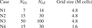
In figure 12, the predicted cavitation regime of case N1 is shown with 12(a–e) representing a time series. In the time series, it is seen that the model can predict cavitation inception on the cylinder surface. At time  $T_2$, the cavity HC1 starts to grow from the sharp edge of the cylinder, while a second spanwise cavity, HC2, is already developed downstream. Meanwhile, we have a shedding cavity HS1 further downstream. At time
  $T_2 + 5\Delta T$, HC1 is growing while HS1 is almost a stretched streamwise vortex. At
  $T_2 + 15\Delta T$, HS1 is still resolved as cavitating, without a fast collapse (as seen with the Eulerian model, figure 11), and the cavity HC2 is shedding. Finally at
  $T_2 + 30\Delta T$, HC1 is a developed spanwise cavity similar to HC2 at time
  $T_2$. Figure 12( f) represents a different instance with a dense cavity in the wake area, similar to figure 10(e). Apart from the cyclic shedding pattern, in figure 12, we can see transverse cavities (as the flow separates on top of the cylinder) as well as dispersed vapour structures further downstream, which were found in the experimental results but were not captured by the Eulerian model.
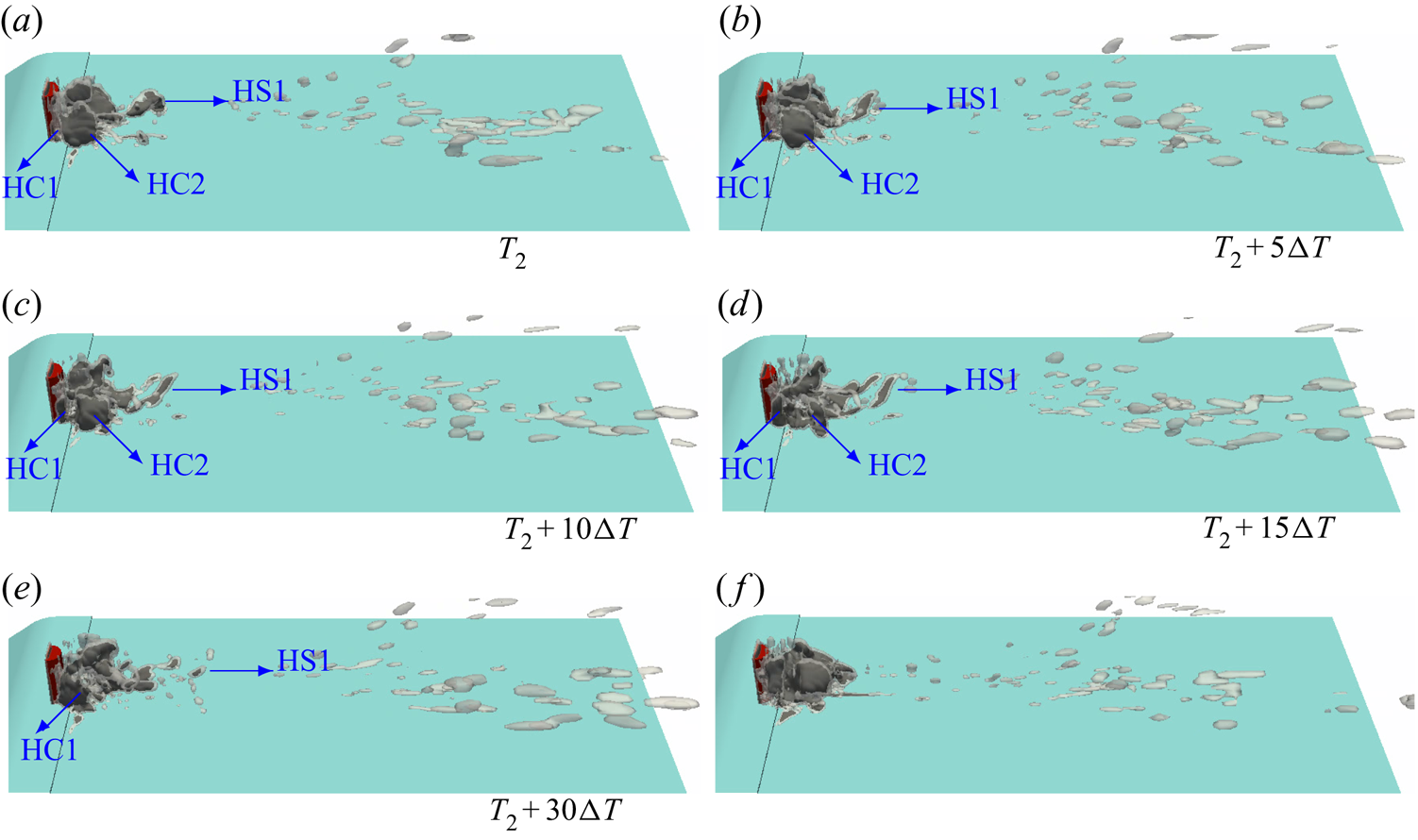
Figure 12. Contours of liquid volume fractions of 0.9 (light gray) and 0.5 (black) obtained by the hybrid model. Panels (a–e) represent a time series. Panel ( f) shows an instance with more vapour volume. Here, HC1 and HC2 represent two spanwise cavitating vortices and HS1 is a streamwise cavitating vortex.
For further comparison between the Eulerian and hybrid models results, in figure 13 the side-view average cavity pattern of all numerical simulations are compared with the experimental result. As it is not possible to measure the liquid volume fraction from the diffuse black and white averaged image of the experiment, for a qualitative comparison, we plot two iso-surfaces of the numerical results. In the figure, the black colour is the iso-surface of a liquid volume fraction of 0.6, while the transparent grey colour represents the volume fraction of 0.9. The experimental image is averaged over a time period of 0.25 s while the numerical results are averaged over a period of 0.025 s, which corresponds to approximately  $2\times 10^5$ time steps for each case. Therefore, we do not expect the numerical figures to fully represent the average flow, although 0.025 s is approximately 10 times larger than the flow characteristic time. However, considering that we cannot extract a quantitative volume fraction from the experiment, the numerical figures can be used for a qualitative comparison. From the averaged figure, the Eulerian model limitation in resolving the cavities in transverse vortices (in the near-wake area) as well as the shedding structures is now more obvious. The height and length of the cavity are smaller than the real results, and even in the average cavity, the liquid volume fraction is considerably lower, as no volume fraction of 0.6 is seen from the Eulerian model. In fact, from the averaged numerical results, we did not see any cavity structure with a liquid volume fraction lower than 0.75 for the Eulerian model.
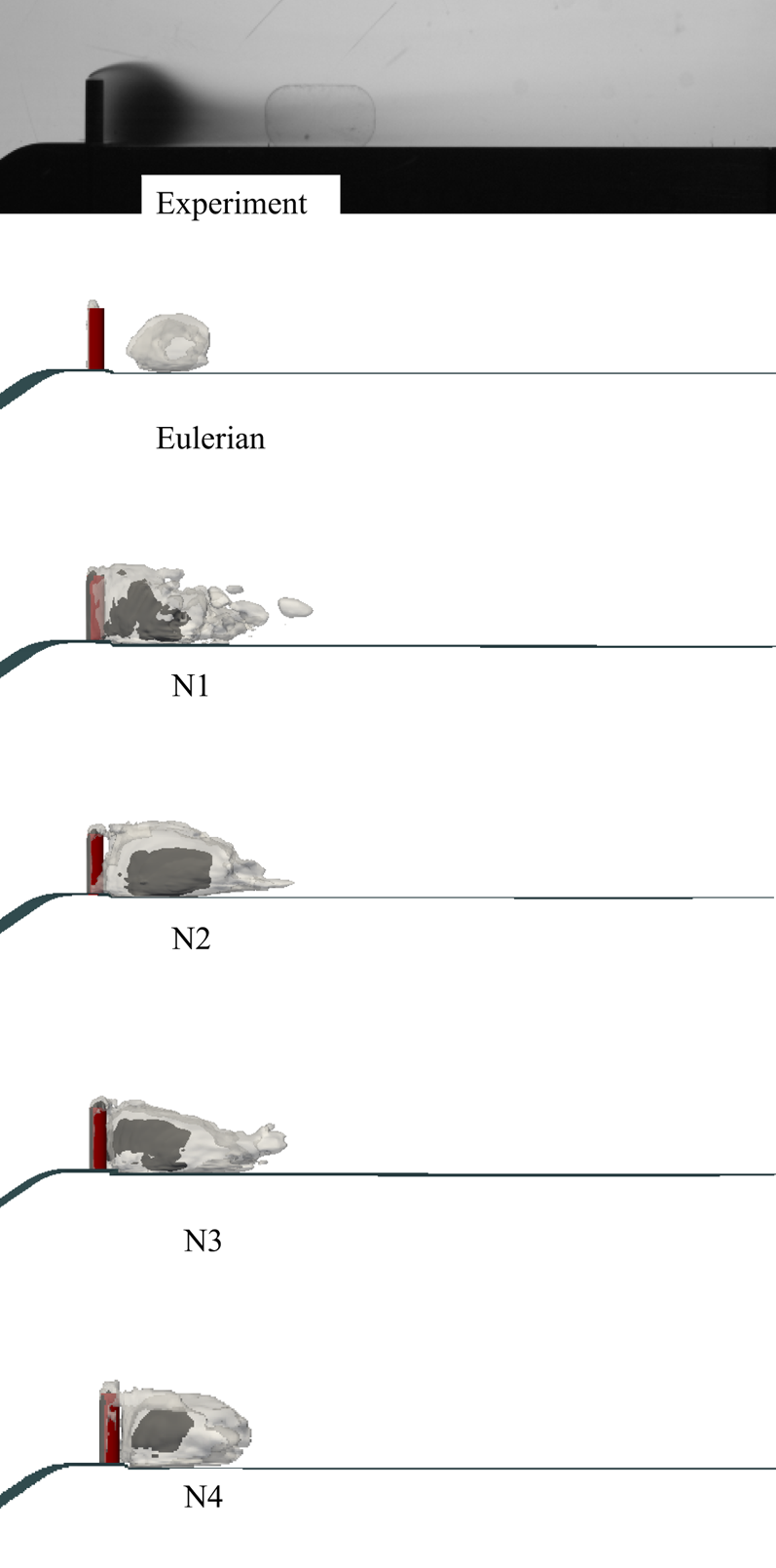
Figure 13. Comparison of the averaged cavity pattern of different numerical simulations (Eulerian and hybrid N1–N4) with experiment. Numerical cavities are shown by contours of liquid volume fractions of 0.9 (light grey) and 0.6 (black).
With the hybrid model, however, we can see considerably more cavities including transverse cavities, higher spanwise cavities starting on the body surface, shedding structures and more vapour content in the core of the averaged cavity (figure 13, rows 3–6). As will be explained later in the discussion of the flow field, such an improvement is not only a result of capturing the sub-grid structures by the Lagrangian model but also the interactions between vapour structures and the continuous flow at different scales. It is important to note that the hybrid model results in a considerable improvement even with a lower mesh resolution (Case N4). This can significantly reduce the computational cost. It is worth mentioning that the number of computational processors used for the coarse grid was 1/3 that used for the main grid while the required time for calculating each time step was reduced to 2/3. Furthermore, the computational time required for each usual time step of the hybrid simulation with the main grid was approximately 20–30 % more than the corresponding one for the Eulerian model, and changing the threshold numbers ( $N_{EL}$ and
  $N_{LE}$) between the hybrid cases did not lead to considerable variations in the computational costs.
Apart from the underestimated cavitation inception on the body surface, the Eulerian mixture model can have an issue with inception prediction in another region as well, which is the lower wall on the left and right sides of the bluff body. In the earlier simulations for a lower cavitation number of 0.64 (Ghahramani et al. Reference Ghahramani, Jahangir, Neuhauser, Bourgeois, Poelma and Bensow2020), we found that when the cavity volume in the wake area increases, the numerical simulation predicts some spurious cavities on the lower wall that are not observed in the experiments. In figure 11(f) also, we see that at an instance of the Eulerian result with more vapour volume in the cylinder wake, some spurious vapour is overestimated on the left and right corners of the lower wall upstream of the bluff body. For further evaluation with a higher vapour volume in the wake, figure 14 shows an instance of a hybrid model simulation which has a slight difference with the earlier results. This simulation has the same parameters as case N3; however, the Eulerian to Lagrangian transition algorithm is deactivated on a part of the lower wall which is on left side of the cylinder. Therefore, in the area enclosed by the red square, the cavities were modelled by the Eulerian model and everywhere else the hybrid model was used. The figure also shows the small Lagrangian bubbles whose sizes are scaled by 400  $R_0$ for visualization purposes (
 $R_0$ is the radius of the equilibrium nucleus for each bubble). As seen in the figure, at such a moment, the Eulerian model predicts spurious vapour on the lower wall, while on the opposite side, the initial cavities are transformed to very small Lagrangian bubbles which do not grow spuriously. The source of spurious vapour generation of the Eulerian model will be explained in § 5.
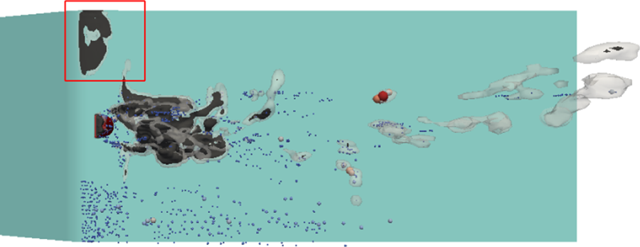
Figure 14. Overestimation of cavitation inception on the lower wall by the Eulerian model (on the left of the cylinder) compared with the hybrid model prediction with no spurious cavity (on the right of the cylinder).
The results of cases N1–N4 share a lot of similarities and, with the average cavity pattern in figure 13, they predict almost similar cavity length and size with a higher vapour density at the core. However, it is not possible to make an accurate comparison between the cases from this figure as we do not have numerical values of the experimental vapour distribution and the numerical results are averaged over a shorter time range. In figure 15, instantaneous results of different cases are shown for comparison. It should be mentioned that the performances of the model are very similar in the estimation of the cyclic cavity pattern that is explained for case N1 in figure 12 and more results from case N2 will be shown later. However, the examples of each case in figure 15 are specific instances, which better represent the characteristics of the corresponding case. For case N1, it is seen that the shed cavities downstream are less resolved and smaller compared with cases N2 and N3. This arises from the lower resolution of Eulerian cavities before their transformation to the Lagrangian bubbles in case N1. When an Eulerian cavity is less resolved, its inertia and collapse rate might not be well estimated, which leads to a less accurate initialization of Lagrangian bubbles. In fact, sometimes the shed cavities at the end of the wake area might be very small and almost collapsed before transformation to the Lagrangian framework. Therefore, there is not a sufficient opportunity to improve the estimation of cavity inertia or avoid its complete collapse by taking into account other effective parameters from the Rayleigh–Plesset equation.
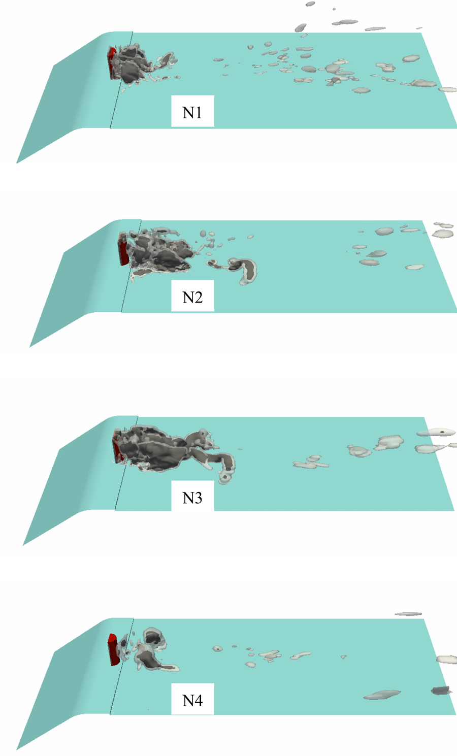
Figure 15. Instantaneous cavities predicted by different cases of the hybrid simulation.
Comparing the second and third cases, we see that case N3 predicts larger cavities downstream and sometimes with better resolution. However, the issue with case N3 is that by using large threshold numbers, sometimes we may end up with dense cavities in the Lagrangian framework, which may exceed the near packing limit. In such a case, the inherent assumptions for the applied models for calculation of bubble transport and dynamics might be violated, which leads to less accurate results. During the initialization of our simulations, this case was less stable and it seemed that the transport of some of the detached cavities at the end of the wake were not calculated appropriately. By comparing the cases N1–N3, it seems that while the model has satisfactory performance in the wake area and the cavity development, the prediction of shedding cavities downstream can vary by changing the threshold numbers of the Eulerian–Lagrangian transition. Additionally, considering the non-uniform mesh in typical cavitation problems, for further improvements of the solver, it is suggested to use a more robust transition criteria rather than only the relative size of the cavity. This will be a topic of future study.
In case N4 of figure 15, it is seen that while the cavitation starts from the body surface and the cavities in the wake region do not have an unrealistic fast collapse, the larger cavities have less vapour content compared with the corresponding structures in the earlier cases with a fine grid. It is obvious that this resolution is not sufficient for a pure Eulerian simulation, and when a Lagrangian cavity grows and is transformed to the Eulerian framework, it will not be sufficiently resolved afterwards. Case 4 shows that to obtain sufficiently accurate results, both Eulerian and Lagrangian parts of the solver should model the corresponding structures with good accuracy.
In summary, by comparing the different cases, it can be concluded that the hybrid model can improve the cavitation inception and the modelling of the sub-grid structures in the wake area and the unrealistic fast collapses of small cavities are avoided by taking into account the cavity inertia more appropriately. For a more satisfactory prediction, it is important that the cavities are well represented in both frameworks. Especially during an Eulerian to Lagrangian transition, it is important that the earlier Eulerian cavities are well modelled with reasonable estimation of the cavity collapse rate for a correct initialization of the Lagrangian bubbles. In the next section, the multi-scale cavitation development around the bluff body is investigated in further detail using the results of case N2, which have a better estimation of shedding cavities compared with cases N1 and N3, as explained above.
5. Multi-scale cavitation development
In § 4.2, the cavitation regime was described based on the high-speed images of the experimental test (Ghahramani et al. Reference Ghahramani, Jahangir, Neuhauser, Bourgeois, Poelma and Bensow2020). Although we can identify cyclic cavity shedding from the wake area and the growth of spanwise cavities from the experimental results, it is not possible to explain the cavity development in each cycle from the high-speed images. In particular, it is not clear how the cavities evolve in each cycle and why, at some instances, we have a low vapour volume behind the cylinder (figure 10f), while at other times, the wake area is filled with vapour (10e). Therefore, in this section, we investigate further details of the flow field behind the sharp-edge bluff body using the hybrid model results.
To investigate the flow field, we start with a simulation of a non-cavitating single phase flow at the same condition. Such a simulation can be performed by deactivating the cavitation model and because only the pressure differences matter in non-cavitating incompressible flow, there is no need to modify the pressure values at the boundaries or in the initial condition. In figure 16, the vortices at two instances of the non-cavitating flow are depicted based on the iso-surfaces of the  $Q$-criterion. The
  $Q$-function calculates the second invariant of the velocity gradient tensor and the
  $Q$-criterion defines a vortex as a connected fluid region with a positive second invariant of velocity gradient; therefore, to represent the vortices, we need to plot the regions with
  $Q \geq 0$. As there are many vortex structures in the wake region, only higher strength vortices with
  $Q \geq 10^{7}$ s
 $^{-2}$ are depicted in the figure. The iso-surfaces are coloured based on the local pressure values on a logarithmic scale. In figure 16, the colour scale is adjusted in such a way that the pressure values below
  $p_v = 2320$ Pa (potentially cavitating regions) are coloured as the vapour pressure; as stated, for incompressible flows, only the relative pressure matters. From the distinct vortices behind the cylinder in figure 16, two points can be concluded: first, in the near-wake area, immediately after the cylinder, the pressure is still above the saturation vapour pressure. It can drop to the vapour pressure in the spanwise vortices, which have moved a certain distance downstream. Second, the pressure drop starts from the bottom of the spanwise vortices on the lower wall, and for some of the vortices, we see that only the lower part has a pressure below 2320 Pa. The vortex pressure may continue to decrease as it moves downstream. In addition, sometimes the head of a spanwise vortex is stretched through its interaction with transverse vortices and other spanwise structures. As a result, the core pressure of the vortex may decrease further while its head is tilted in the streamwise direction.

Figure 16. Vortex structures of non-cavitating flow with  $Q \geq 10^{7}$ s
 $^{-2}$, coloured by pressure values. Panel (a) shows a distance between the cylinder and the first low-pressure vortices, while (b) shows a pressure drop in a streamwise vortex.
When the flow cavitates, at instances when the vapour volume in the wake is low, we see that some of the spanwise vortices, similar to those in figure 16, start to cavitate and their vapour content increases with time. At such times, the vapour volume at the near-wake region immediately after the body is negligible and the spanwise vortices cavitate gradually after travelling a distance from the body. Figure 10( f) from the experimental results is a good example of such an instance. In this figure, we see a low vapour volume behind the cylinder and a spanwise vortex (SC1) is cavitating from the bottom, while its upper part is stretched in the streamwise direction. When a vortex is stretched, its core pressure drops, which can cause cavitation. From a simulation point of view, the Eulerian model can capture such instances to some extent. In figure 11, we can see spanwise vortices that partially cavitate in the lower part. However, the issue with this model is that the numerical cavities collapse too early, which can either be owing to the spatial resolution or the model incapability in representing the cavity inertia. Therefore, the Eulerian model cannot capture further increase of the vapour volume.
As the vapour volume increases, the vortex pattern of the two-phase flow as well as the wake pressure field change. This increases the vapour content of spanwise vortices in the near-wake area. At first, only the lower parts of the vortices cavitate, but after a while, we see that as the flow separates from the sharp edges of the body, the entire evolving vortex is filled with vapour. A good example of such an instance is the vortex C31 in figure 9(a,b). The evolving vortex then moves downstream with its increasing vapour content. If two subsequent spanwise cavities do not grow so much that the earlier cavity is shed before the second one arrives, we can see distinct spanwise cavities similar to the depicted time series in figures 9 and 12.
However, sometimes two (or more) subsequent vapour structures grow and merge to a larger cavity. The large cavity in figure 10(e) represents such a structure. To understand this process, in figure 17, a time series of the flow at such an instance is depicted. In the figure, we have various interacting structures and the colours are adjusted to increase the contrast. We see Lagrangian bubbles (coloured in purple and scaled based on their diameters), iso-surfaces of  $Q = 10^{7}$ s
 $^{-2}$ (coloured in transparent cyan) and iso-surfaces of Eulerian cavities with
  $\alpha = 0.9$ (coloured in lime green). Additionally, for visualization purposes, the vortices on the lower wall and the opposite side of the cylinder are excluded in the figure. At this time, we have a large cavity downstream and, between this cavity and the cylinder, there are three spanwise vortices, V1, V2 and V3. At time
  $T_3$, a large part of V1 cavitates, while inside V2, we see only Lagrangian bubbles. As the vortices move downstream, at
  $T_3 + 2.5 \Delta T$, the cavity in the core of V1, called C1, is growing and we see that the lower part of V2 starts to cavitate, C2; by this, we mean that the Lagragian bubbles grow so much that they are transformed to Eulerian cavities. At time
  $T_3 + 5 \Delta T$, it is seen that the vorticity of V3 is reduced as it has more vapour content; at the same time, C2 is growing. Finally, at
  $T_3 + 10 \Delta T$, C2 has expanded so much that the vorticity of V2 is reduced such that
  $Q < 10^{7}$ s
 $^{-2}$. From this time series, we see that similar to the earlier depicted instances, cavitation starts at the lower part of the spanwise vortex and then it is expanded to the upper part. It is worth mentioning that the vorticity reduction in the vapour zone arises from the mass transfer between the phases as well as the density variation in the two-phase flow, as explained by the vorticity equation in the paper by Gnanaskandan & Mahesh (Reference Gnanaskandan and Mahesh2016).
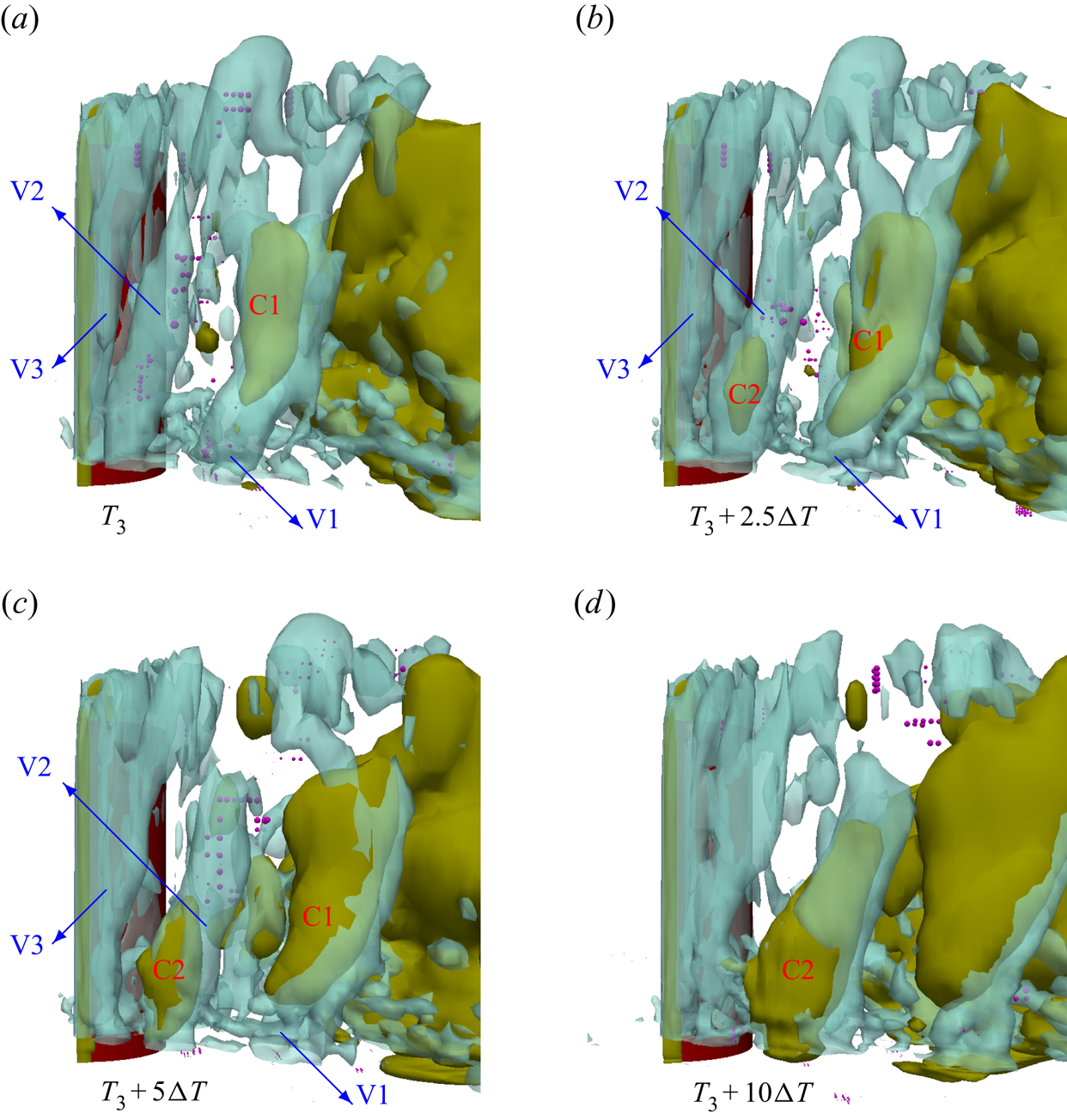
Figure 17. Cavitation development in two subsequent spanwise vortices between a large cavity and the bluff body. Panels (a–d) represent a time series. The vortices are plotted with  $Q \geq 10^{7}$ s
 $^{-2}$ (coloured in cyan); the vapour structures include Eulerian cavities (coloured in lime green) and small Lagrangian bubbles (in purple).
By comparing figures 16 and 17, we see that for the non-cavitating flow, the pressure drops and stays at the vapour saturation value in some of the spanwise vortices but not all of them. The same scenario applies to the earlier depicted instances of the cavitating flow with low vapour volume in the wake region. However, in the depicted current time series of figure 17, it is seen that two subsequent spanwise vortices cavitate and their vapour contents keep growing from the cylinder surface until they coalesce with each other and with the larger downstream cavity. Therefore, the expansion of cavities in the wake region is not only from the growing of large-scale structures but also from the inception of other small-scale vapours and their coalescence with the earlier cavities. This does not include only the spanwise cavities but also other vapour fragments around the large cavities, as we see in figure 17. Such small-scale structures can be generated in the core of other vortices or be detached from a big cavity.
The other important point is that when the vapour volume is large, the flow vorticity decreases significantly in the wake area, and the vortices and pressure field have substantial differences with a non-cavitating flow. The pressure value in (almost) the entire wake area is equal to the vapour pressure (see figure 19d, which will be discussed later). In general, it can be stated that the energy head is substantially lower in this region compared with the surrounding. In figure 18, an axial velocity contour corresponding to such an instance is plotted over a section normal to the cylinder. The 2-D plane crosses the cylinder at its half-height and the range of the colour legend is reduced to increase the contrast. We can see that because of the pressure (or energy head) difference with the surrounding as well as the interaction with the shedding vortices, a jet flow moves toward the bluff body. This jet mainly comes from the end of the cavity and partially condenses the vapour structures. A few time steps later, the vapour volume decreases substantially, the cavitation occurs mainly in the spanwise vortices and the cycle repeats. In an earlier study, it was shown that at lower cavitation numbers ( $\sigma \leq 0.64$), a fixed cavity attached to the cylinder is formed in the wake area (see figure 17 in the paper by Ghahramani et al. Reference Ghahramani, Jahangir, Neuhauser, Bourgeois, Poelma and Bensow2020). For that case, the attached cavity is so long that the jet flow can be seen as a clear reverse flow inside the vapour zone that can cause temporary detachment of the fixed cavity from the cylinder. For the current case, we see more frequent but smaller reverse jets, which cause partial collapses of the vapour.
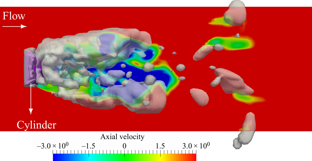
Figure 18. Instantaneous axial velocity contour in a 2-D plane at  $z = 0.5H$ during partial collapse of a large cavity (coloured in grey). The velocity colour legend range is limited to increase contrast.
Using numerical results at  $\sigma = 0.64$, it was shown by Ghahramani et al. (Reference Ghahramani, Jahangir, Neuhauser, Bourgeois, Poelma and Bensow2020) that inside the large fixed cavities in the wake area, the axial velocity is often negative and the reverse jet usually increases the absolute value of this negative velocity. The exact physical reason for the reverse jet is not completely clear, but it seems that this flow occurs because of pressure fluctuations at the trailing edge of the large cavity. More simply, we know that in a single phase flow around a bluff body, the pressure field around the body fluctuates due to the detachment and shedding of vortices, which leads to a temporal variation of the drag force on the body. For the current case, at the instances with a low vapour volume in the wake, the vortices are shed from the cylinder edges. By increasing the vapour volume, the flow vorticity decreases substantially inside the cavity (as will be explained later in figure 19d) and vortex shedding occurs mainly at the trailing edge of the large cavity, instead of the cylinder edges. This, in turn, shifts the location of the corresponding pressure fluctuations (responsible for temporal load variations in single phase flows). Such fluctuations at the trailing edge and the lower pressure inside the cavity can be the source of the reverse jet. Further details in this regard can be found in the paper by Ghahramani et al. (Reference Ghahramani, Jahangir, Neuhauser, Bourgeois, Poelma and Bensow2020). In summary, it can be stated that despite the general periodicity of the flow in average, in each cycle, the flow is very unsteady with continuous variations in the length scale of the cavities. Furthermore, the vapour structure is not only a function of generated vortices from upstream flow separation, but also dependant on the flow history and the downstream cavity pattern.

Figure 19. A comparison between the flow field at two instances with low and high vapour volumes in the wake area. (a,b) Cavity structures; (c,d) vortical structures coloured by pressure; (e, f) 2-D streamlines and pressure contours on a plane parallel to the flow direction; (g) temporal pressure variation at point A.
In the previous study of Ghahramani et al. (Reference Ghahramani, Jahangir, Neuhauser, Bourgeois, Poelma and Bensow2020), it was also shown from numerical results that for a lower cavitation number ( $\sigma = 0.64$), the large fixed cavity that is developed in the wake area affects the vorticity and modifies the flow pattern downstream of the cylinder. Their simulation was performed using an Eulerian model and, as stated, it overestimated the cavities on both sides of the lower wall upstream of the cylinder, which prevents a correct investigation of the cavitation effect on the upstream flow. Using the hybrid model in this study, we show that the vapour structures can change the main flow pattern at a higher cavitation number with a cyclic cavity pattern as well, but this effect is more considerable when the cavity volume is higher. Furthermore, as the overestimation of cavitation inception is avoided with the hybrid model, it is now possible to analyse the cavity effect on the flow at upstream locations.
In this regard, figure 19 shows two different instances of the flow at which the vapour volume is low (left column) and high (right column). Figure 19(a,b) shows the cavity pattern for each case. Figure 19(c,d) shows the flow vortices via the iso-surfaces of  $Q = 10^{7}$ s
 $^{-2}$. As explained, with the higher vapour volume, the flow vorticity in the wake area decreases. The iso-surfaces are coloured with the local pressure value on a logarithmic scale. By comparing the two instances, we find that with larger cavities, the pressure in front of the cylinder is lower. This can be specifically seen in the pressures of the ring vortices just in front of the cylinder base. In the earlier experimental investigation, it was seen that at low cavitation numbers (
 $\sigma \leq 0.64$), a ring vortex cavitates periodically in front of the cylinder (see figure 16 in the paper by Ghahramani et al. Reference Ghahramani, Jahangir, Neuhauser, Bourgeois, Poelma and Bensow2020) and from the numerical results, we now have a more clear understanding of the process. In addition, on the left and right sides of the lower wall, we see considerable variations between the two instances in pressure values and vorticity. In fact, for the higher cavity volume, the pressure falls below the saturation value at some area. To further our understanding, the streamlines and pressure contours in a surface at point A are plotted in figure 19(e, f). Point A is depicted in figure 19(b) and the 2-D surface is parallel to the flow direction. From the streamlines, it can be seen that for the higher cavity volume, the flow separates at the end of the sloped wall, while it stays attached to the wall for the other case. The flow separation leads to a local pressure drop on the wall and induces more vorticity. However, as the pressure increases when the cavity volume changes later, no cavitation occurs on the lower wall. From our earlier experience, at lower cavitation numbers (e.g.
  $\sigma = 0.56$), when the cavity volume in the wake area is considerably larger, temporary and unstable cavities are seen on the lower wall.
From a simulation point of view, it is now possible to explain the issue with the Eulerian model in cavitation prediction on the lower wall. The mass transfer source term in this model is mainly a function of the difference between flow pressure and vapour saturation pressure (3.7). As the local pressure drops below the vapour pressure on the lower wall, the liquid cavitates. By decreasing the liquid volume fraction, the mass transfer source term becomes bigger, which leads to an increase in the vapour volume and a further decrease in the surrounding pressure. Therefore, after a short period of time, a sheet cavity develops on the wall. However, we know that, in reality, the size of a bubble (nucleus) does not change rapidly after a pressure drop, because of its inertia. Furthermore, the bubble surface tension is another parameter which has an opposite effect, especially at small scales. These two parameters are taken into account in the Rayleigh–Plesset equation, via the first and the last terms (3.21). When we use the hybrid model, after the pressure drop on the lower wall, the initially small Eulerian cavity is transformed to Lagrangian bubbles as it is not resolved by a sufficient number of cells. Then, in the Lagrangian framework, the mentioned effects are taken into account, which leads to a more accurate estimation of the bubble growth rate. Figure 19(g) shows the temporal variation of the pressure at point A on the lower wall. As we see, the pressure varies over time and it does not stay below the saturation value for a continuous long period. Therefore, when there is a small bubble at point A, for example, before it can grow substantially, either the pressure increases or the bubble moves downstream and leaves the small low-pressure region.
To further analyse the effect of the inertia and surface tension of the bubbles at the inception phase, in figure 20, these effects are plotted for the corresponding instances. The left and right columns of this figure correspond to the left and right columns of figure 19, respectively. In figure 20, only the bubbles on the right hand side of the cylinder are depicted, and their size is scaled by  $40R$ for visualization purposes. By comparing figures 20(a) and 20(b), it is seen that when the flow pressure decreases during separation, more Lagrangian bubbles are created from small Eulerian cavities. Figure 20(a–d) show the bubble inertia terms on the left hand side of (3.21). The growth rates (
 $\dot {R}$) of some of the small bubbles are clearly larger when the pressure drops during separation. These bubbles are marked by an enclosing red box. However, the second temporal derivatives of the radius for the same bubbles have large negative values (figure 20d). Figure 20(e, f) clearly shows the order of surface tension of small bubbles, compared with the other two terms, which can considerably counteract a sudden local pressure drop around the bubbles (see (3.21)). As stated previously, most of the common finite mass transfer models in the literature (including the current Eulerian model) ignore the surface tension (
 $2\sigma /{R}$) and second derivative (
 $R\ddot {R}$) terms, and the mass transfer rate is a rough simplification of the Rayleigh–Plesset equation. As a result, after a pressure drop, the mass transfer rate increases (similar to bubble growth rate shown in figure 20b), while neither the vaporization rate is correctly resolved nor the effective force balance on the cavity interface is accurately modelled.
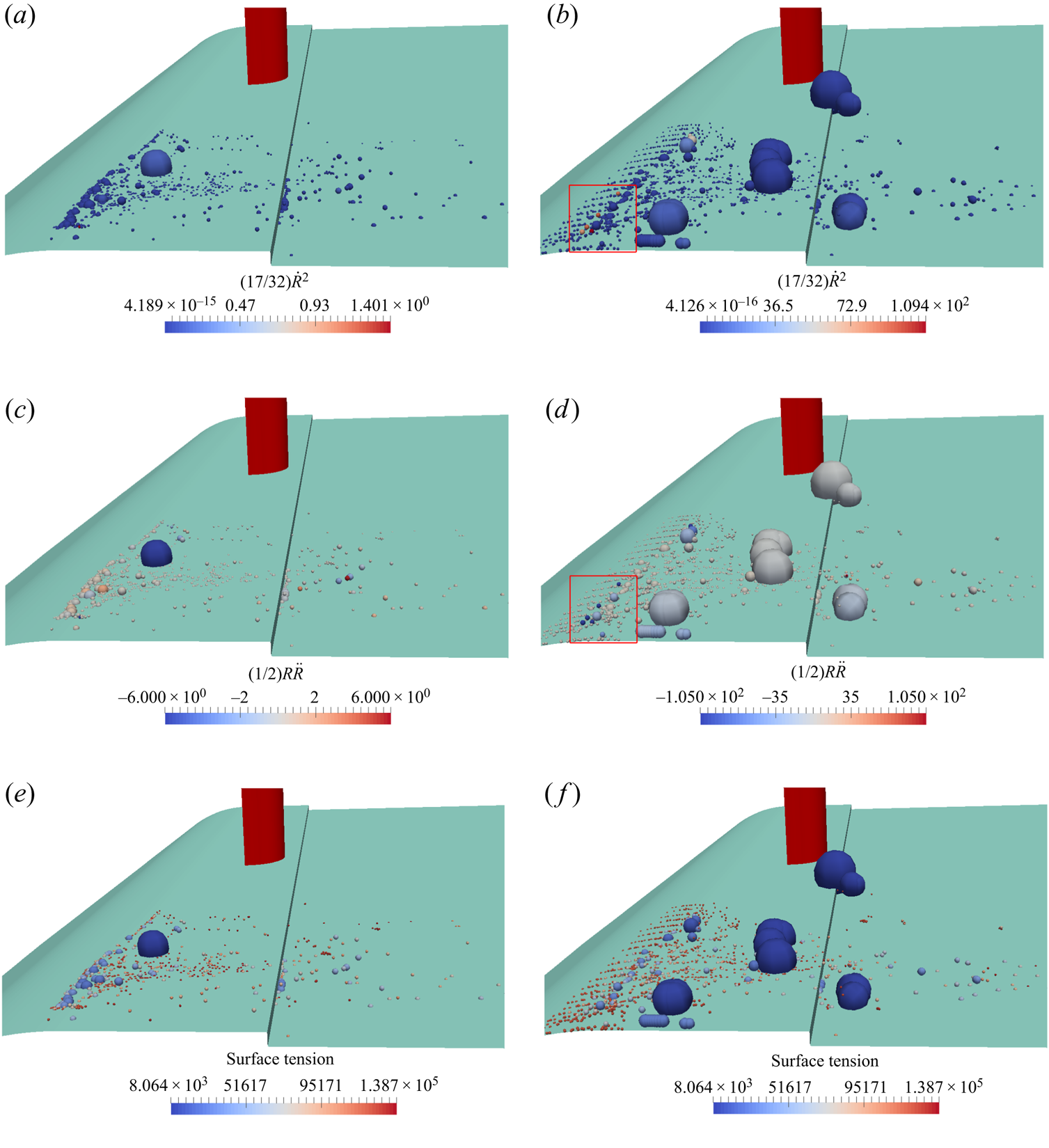
Figure 20. A comparison between inertia and surface tension of bubbles at two instances with low and high vapour volume in the wake area. (a,b)  $\frac {17}{32}\dot {R}^2$; (c,d)
  $\frac {1}{2} R\ddot {R}$; (e, f)
  $2\sigma /{R}$. Panels (a), (c) and (e) correspond to figure 19(a); (b), (d) and ( f) correspond to figure 19(b). The size of the bubbles are scaled by
  $40R$.
6. Conclusions and outlook
In this study, a multi-scale cavitation problem is investigated using a newly developed hybrid model. The model is developed by coupling an Eulerian mixture with a Lagrangian bubble model. Compared with the earlier hybrid models, the coupling algorithm is more compatible with the flow physics, and the mass, momentum and kinetic energy of the cavities are conserved during the Eulerian–Lagrangian transition. Furthermore, new submodels were introduced in the Lagrangian model to consider bubble–bubble interactions and break-up, the bubble–wall boundary condition, void handling scheme and taking into account the local pressure effect on bubble dynamics. The new implementations lead to further enrichment of the Lagrangian tracking, which makes the model applicable to densely 3-D cavitating flows in real scales. For the Eulerian cavities, we considered an incompressible flow and a transport equation model, motivated by the lower computational cost for the large-scale application; however, the coupling algorithm can be used for compressible models to take into account the relevant flow effects in other applications. The obtained results show considerable improvements in the numerical simulation of multi-scale cavitation compared with the commonly used Eulerian mixture model.
The improvements include capturing the cavitation inception on the surface of the bluff body, avoiding spurious cavities on the lower wall and modelling the sub-grid vapour structures, not only in the wake area around the larger cavities but also the shedding vortices and disperse clouds downstream. Our results show that the improved performance can be achieved even with noticeably lower mesh resolution, which can reduce the computational costs. The model comparison further clarifies the numerical issues with the Eulerian models. In addition to the well-known higher dependency on the grid resolution, the common Eulerian models do not give an appropriate estimation of the cavity inertia, and as cavitation is modelled only based on the pressure variations, the cavity dynamics is highly dependant on temporal variations of the pressure. As a consequence, fast temporal pressure variation causes spurious cavitation on the lower wall and a higher condensation rate in the wake area. For future improvements of the Eulerian models, one suggestion is to include the flow history effect or pressure variation rate in cavitation modelling. Another suggestion is to implement the cavity inertia effect (e.g.  $\dot {V}$ or
  $\ddot {V}$) in the condensation/vaporization rates.
The numerical results also show that the cyclic cavity development and shedding in the wake area is a very unsteady process with various interactions between the large- and small-scale cavities as well as the continuous flow. The larger cavities are not only developed from growing of a spanwise cavitating vortex, but also the vaporization of other vortices and the smaller vapour structures at sub-grid scales and the coalescence of these structures. Such vaporization and the coalescence probability are dependent on the flow vorticity and pressure fields in the near-wake area which are, in turn, influenced by the downstream cavities. With lower vapour volume, only a fraction of spanwise vortices cavitate from their lower part and after travelling a minimum distance from the body. With increasing vapour volume, the cavitation starts from the bluff body surface with more frequent vaporization of spanwise and transverse vortices. At larger volumes, the generated cavity can considerably influence the flow upstream of the cylinder, which explains the periodic cavities on the lower wall and ring-shaped vortices in front of the body that have been reported for lower cavitation numbers.
Finally, a comparison between different cases of the hybrid simulation further clarifies the model characteristics. From this comparison, we conclude that for satisfactory simulations, both Eulerian and Lagrangian parts should model the corresponding structures with sufficient accuracy. In general, the current hybrid framework can be applied to a wide range of cavitating flows with extensive range scales. While the primary intention has been to improve the representation of multi-scale problems, it is possible to apply the same framework to smaller scales (in which the cavities are mainly represented by the Lagrangian formulation), as well as large-scale developed cavities (where the Eulerian equations are mainly solved). However, before choosing any model, the considered hypothesis in the model formulation should be taken into account. In this study, we used a common Eulerian model and the improvements were more focused on the Lagrangian modelling and the transition algorithm. To increase the model accuracy, the Eulerian model can be improved based on the above-mentioned suggestions. Additionally, a hypothesis considered in the model is that thermodynamic effects are neglected and the energy equation is not solved, as the intended application has been large-scale industrial cases, such as the current problem, and hydraulic systems. It is worth emphasizing that this hypothesis is related to the selected Eulerian model in the current study, and the hybrid framework can be extended to consider thermodynamic effects with suitable Eulerian models. Furthermore, for a more numerically robust transition between the Eulerian and Lagrangian frameworks, the transition criterion can be defined based on a more suitable parameter that considers non-uniformity of domain discretization. Another feature of the current hybrid model is that the cavitation inception is first estimated at low-pressure regions, which limits the predictions to the capabilities of the Eulerian mass transfer models. The vapour inception can be based on free nuclei in the liquid and on solid walls. Although the inception is well represented in the current problem, introducing nuclei can make the inception process more independent from the Eulerian simulation and adds the possibility to consider liquid quality, and this is the subject of ongoing research. In addition, the hybrid model can be used in erosion/noise estimation of cavitating flows. This can be achieved by either incorporation of the radiated acoustic pressure wave arising from bubble collapse and rebound (see e.g. Eskilsson & Bensow Reference Eskilsson and Bensow2015) or through coupling of the Lagrangian model with a compressible model. Accounting for the compressibility effect (both in the mixture model and the Rayleigh–Plesset equation) is also needed in the investigation of the flow field in micro-scale applications.
Acknowledgements
The authors would like to thank Dr. A. Asnaghi for the interesting discussions about the numerical models.
Funding
This work is partly funded through the EU H2020 project CaFE, a Marie Skłodowska-Curie Action Innovative Training Network project, grant number 642536. It was also funded by Kongsberg Maritime Sweden AB through the University Technology Centre in Computational Hydrodynamics hosted at the Department of Mechanics and Maritime Sciences at Chalmers. The computations were performed on resources at Chalmers Centre for Computational Sciences and Engineering (C3SE) and at National Supercomputer Centre (NSC) provided by the Swedish National Infrastructure for Computing (SNIC).
Declaration of interests
The authors report no conflict of interest.
Appendix A. A brief explanation about Lagrangian submodels
In this appendix, more details of the Lagrangian submodels are provided for the interested reader. It also includes an overview on some of the other available models in the literature and gives the rationale behind developing or choosing the submodels that are introduced in the paper.
A.1. Rayleigh–Plesset equation
As stated before, the inherent assumptions of the original form of the Rayleigh–Plesset equation mean that it cannot sufficiently estimate bubble dynamics in complex and real problems, in which bubbles are surrounded by other cavity structures and flow boundaries. Therefore, various improved versions of this equation have been introduced in the literature to address such limitations. In some cases, consideration of local flow effects on bubble dynamics has been attempted by replacing the infinity pressure in the Rayleigh–Plesset equation with the local flow pressure on the bubble interface or near it and, to compensate for such a simplification, some correction terms have been added to the equation. For example, Hsiao et al. (Reference Hsiao, Ma and Chahine2017) suggested a slip velocity correction term based on the bubble–flow velocity difference and Giannadakis et al. (Reference Giannadakis, Gavaises and Arcoumanis2008) proposed another correction term based on local turbulence quantities. Fuster & Colonius (Reference Fuster and Colonius2011) developed an extended Rayleigh–Plesset equation, which accounts for the presence of other bubbles and liquid compressibility effects. This method is able to capture the pressure field generated around the bubble using local information in the vicinity of the bubble and has been tested for the collapse of a bubble cluster. However, the model is too sophisticated for application to real-case complex problems because  $N_{\mathit {cell}}$ equations need to be solved to calculate the potential derivatives of each bubble, where
  $N_{\mathit {cell}}$ is the number of surrounding bubbles in the cell. For incompressible flows, this equation can be simplified considerably to the traditional form of the Rayleigh–Plesset equation with a simple source term to account for the bubble–bubble interaction effect. For the limiting case of a single bubble, this source term is zero and we still have the limitations with the classical form of Rayleigh–Plesset equation that does not apply to non-isolated single bubbles (e.g. near a solid boundary). Therefore, in this study, (3.21) was used, which can consider the local pressure effect and does not have the mentioned limitations, and it has been validated for benchmark test cases (Ghahramani et al. Reference Ghahramani, Arabnejad and Bensow2019).
It is worth mentioning that the introduced localized form of the Rayleigh–Plesset equation (3.21) is similar to the LVARP equation (locally volume-averaged Rayleigh–Plesset equation) developed by Seo, Lele & Tryggvason (Reference Seo, Lele and Tryggvason2010) but with different coefficients for  $R\ddot {R}$ and
  $\dot {R}$. The LVARP equation has been developed in a different way, by considering a local volume around the bubble based on the effective interbubble distance. However, the computation of the control volume radius can be computationally expensive in general non-homogeneous bubble distribution or the equation needs some empirical constants.
A.2. Bubble–bubble collision algorithm
The incidence of collision between bubbles can be determined using deterministic, stochastic or hybrid algorithms. Deterministic algorithms check the trajectories of every two particles,  $i$ and
  $j$, to investigate their possible collision along their path line. Here, the calculation of the trajectories of bubbles/parcels is split into two steps: at first, bubbles are moved based on their equation of motion, and then the occurrence of collisions during the first step is examined for all bubbles/parcels. If a collision is found, the properties of the collision pair are updated based on the collision outcome. When the number of particles is considerably high and the deterministic approach can be computationally expensive, stochastic models can be an alternative. Additionally, when parcels with varying statistical weights are used, the collisions are calculated stochastically. Stochastic models can considerably reduce the computational cost and they are quite common when dealing with a large number of particles. In a given computational volume, the collisions are determined based on the estimated collision frequency of parcels. One of the most commonly used stochastic models is that developed by O'Rourke (Reference O'Rourke1981), in which the collision probability is estimated based on the diameters of the parcels, their relative velocity and the number of bubbles represented by each parcel. Hybrid algorithms are other options, which are a combination of deterministic and stochastic models (e.g. Nordin Reference Nordin2001). However, this algorithm may suffer from serious mathematical inconsistencies (Pischke, Kneer & Schmidt Reference Pischke, Kneer and Schmidt2015). Both the O’Rourke and the Nordin models are available in OpenFOAM.
In the current Lagrangian model, we track parcels directly, rather than using representative distribution functions, and an efficient algorithm based on bubble cell occupancy is used for parcel collision detection, which sufficiently reduces the computational cost. Therefore, the bubble collisions are handled using a deterministic algorithm similar to the work of Breuer & Alletto (Reference Breuer and Alletto2012).
A.3. Other assumptions and simplifications
It is worth mentioning that in addition to the previously stated assumptions in the model development, the Lagrangian method includes some other simplifications as well. For instance, the daughter bubbles after break-up might have different diameters, and bubble–bubble interactions during a time step might sometimes be of other types rather than simple binary interactions. Furthermore, the effect of turbulence fluctuations on small bubble dispersion is not considered in Lagrangian tracking. For this purpose, a fluctuating velocity,  $u'$, should be added to the filtered/averaged velocity in the drag force formula (3.16). To estimate the fluctuating velocity, we need a stochastic model. In some earlier studies, a traditional discrete random walk model has been used. Using this model, which is available in OpenFOAM, can lead to significant errors in anisotropic turbulent flows and it is suggested to use the more appropriate continuous random walk models (see e.g. Dehbi Reference Dehbi2008; Ghahramani et al. Reference Ghahramani, Abouali, Emdad and Ahmadi2014). Because, in this study, we are using an LES model with fine spatial and temporal resolutions, it is acceptable to use the instantaneous filtered velocity in bubble tracking, as followed in similar studies (e.g. Ghahramani et al. Reference Ghahramani, Abouali, Emdad and Ahmadi2017). Implementing a stochastic model can be the subject of a future study. Nevertheless, considering the main numerical assumptions in cavitation modelling and the sophisticated physics of the flow, such simplifications are expected to have minor influence on the final results.
Appendix B. Bubble–wall boundary condition
In this study, the wall boundaries are considered to be rigid and it is assumed that a bubble collides with a wall when the distance between its centre to the nearest wall face becomes equal or less than its radius. When a spherical particle collides with a wall boundary, it may bounce from the wall, stick to the wall or slide over the wall surface. Experiments show that during a bubble–wall collision, a liquid film is present between the bubble and the wall (Podvin et al. Reference Podvin, Khoja, Moraga and Attinger2008). Zenit & Legendre (Reference Zenit and Legendre2009) showed that the behaviour of a bubble colliding with a wall is different from that of a solid sphere, owing to the liquid film and the bubble deformation. In this study, it is assumed that a bubble bounces from a wall.
The velocity of the bubble after collision depends on the direction of the wall normal vector. If the tangential and normal unit vectors of the colliding wall face are denoted by  $t_w$ and
  $n_w$, then the velocity of the bubble before collision can be decomposed as
 \begin{equation} {\boldsymbol{u}}^0_b = {u^{0n}_b} {\boldsymbol{n}_w}+{u^{0t}_b} {\boldsymbol{t}_w}. \end{equation}
Using this decomposition, the after-collision velocity is decomposed as
 \begin{equation} {\boldsymbol{u}}_b ={-}\epsilon_w {u^{0n}_b} {\boldsymbol{n}_w}+ (1-\mu_w) {u^{0t}_b} {\boldsymbol{t}_w}, \end{equation}
where  $\epsilon _w$ and
  $\mu _w$ are the coefficient of restitution and wall friction coefficient, respectively. Here,
  $\epsilon _w$ is given by
 \begin{equation} \epsilon_w = \textrm{e}^{{-}30 \sqrt{Ca/St^*}}, \end{equation}
where  $Ca$ and
  $St^*$ are the capillary and modified Stokes numbers, defined as
 \begin{equation} \left.\begin{gathered} Ca = \frac{\mu u^{0n}}{\sigma},\\ St^* = \frac{4 (\rho_b + 0.5 \rho_l)R u^{0n}}{9\mu}. \end{gathered}\right\} \end{equation}
Appendix C. Detecting collision between a pair of bubbles
To find the collision possibility between each bubble and other bubbles, one method is to loop over all of the other bubbles and examine their trajectories relative to the specified bubble; however, this is a computationally expensive algorithm for dense disperse flows as the number of particles can be quite large. As a more efficient method, in this study, the bubble–bubble collision is detected in a faster algorithm based on the ‘cell occupancy’ concept, see figure 21. Cell occupancy is a property of the grid cells that contains a label list of the bubbles that occupy a cell. Using the cell occupancy, it is possible to examine only the bubbles that are in a reachable distance. Here, we need to define an interaction distance, and the cell occupancy list of the grid cells are transformed between every couple of cells that are within the interaction distance to each other. Consider the red bubble in figure 21, for example. The interaction area is specified by a dashed circle. Having the host cell index of the bubble and the cell occupancies of the other cells in the interaction distance (i.e. within the circle), we can find the index of other bubbles that are within a reachable distance. Then, the collision possibility between this red bubble and the surrounding blue bubbles is examined. In the developed solver, the interaction distance is a user-defined parameter that can be tuned to an appropriate value. This parameter, which is actually the radius of the dashed circle in figure 21, should only be large enough that, for each bubble, the corresponding circle encloses the bubble and its path line within the next time step.

Figure 21. Bubble–bubble collision detection based on cell occupancy.
Following a suggestion found in several earlier studies (see e.g. Chen, Kontomaris & McLaughlin Reference Chen, Kontomaris and McLaughlin1999; Yamamoto et al. Reference Yamamoto, Potthoff, Tanaka, Kajishima and Tsuji2001), the current algorithm relies on the assumption of a constant velocity of the bubble within a time step, which is reasonable for the small time step sizes applied in LES. When potentially colliding bubbles are selected using cell occupancy, based on their relative trajectory, it is first specified if they collide or not. Consider bubbles 1 and 2 with respective initial velocities  ${\boldsymbol {u}}^0_{1}$ and
  ${\boldsymbol {u}}^0_{2}$, and respective radius
  $R_1$ and
  $R_2$, as depicted in figure 22. The initial relative position between the bubbles is
  ${\boldsymbol {x}}^0_{12} = {\boldsymbol {x}}^0_{1} - {\boldsymbol {x}}^0_{2}$. The figure also shows the angle
  $\theta$ between the relative velocity (
 ${\boldsymbol {u}}^0_{12} = {\boldsymbol {u}}^0_{1} - {\boldsymbol {u}}^0_{2}$) and line (1,2) between the centres. The relative travelled distance during the time step
  $\Delta t$ is given as
 \begin{equation} d = |{\boldsymbol{u}}^0_{12}|\cos \theta \Delta t. \end{equation}
Figure 22. Relative motion between potentially colliding bubbles.
It can be shown that a collision occurs within the time  $\Delta t$ if
  $\theta < \theta _c$ and
  $d \geq d_c$, where
  $\theta _c$ and
  $d_c$ are the critical angle and distance given by Vallier (Reference Vallier2013)
 $$\begin{gather} \theta_c = \textrm{arctan} \left(\frac{R_1 + R_2}{\sqrt{{|{\boldsymbol{x}}^0_{12}|}^2 - {(R_1 + R_2)}^2}} \right), \end{gather}$$
 $$\begin{gather}d_c = \frac{{|{\boldsymbol{x}}^0_{12}|} - \sqrt{{{|{\boldsymbol{x}}^0_{12}|}}^2 - (1+{(\tan\theta)}^2)({{|{\boldsymbol{x}}^0_{12}|}}^2-{(R_1 + R_2)}^2)}}{1+{(\tan\theta)}^2}. \end{gather}$$
 If a collision is found between a pair of bubbles, then further calculations should be performed to find the relative velocity and contact angle at the collision instance. According to Breuer & Alletto (Reference Breuer and Alletto2012), the instance within the time step  $\Delta t$ at which collision occurs is estimated as
 \begin{align} \Delta t_{\mathit{col}} =
\Delta t_{min}(1-\sqrt{1-K_1K_2}), \quad K_1 =
\frac{{|{\boldsymbol{x}}^0_{12}|}^2
|{\boldsymbol{u}}^0_{12}|^2}{{({\boldsymbol{x}}^0_{12}\boldsymbol{\cdot}
{\boldsymbol{u}}^0_{12})}^2}, \quad K_2 = 1 - \frac{{(R_1 +
R_2)}^2}{{|{\boldsymbol{x}}^0_{12}|}^2},
\end{align}
\begin{align} \Delta t_{\mathit{col}} =
\Delta t_{min}(1-\sqrt{1-K_1K_2}), \quad K_1 =
\frac{{|{\boldsymbol{x}}^0_{12}|}^2
|{\boldsymbol{u}}^0_{12}|^2}{{({\boldsymbol{x}}^0_{12}\boldsymbol{\cdot}
{\boldsymbol{u}}^0_{12})}^2}, \quad K_2 = 1 - \frac{{(R_1 +
R_2)}^2}{{|{\boldsymbol{x}}^0_{12}|}^2},
\end{align}
where  $\Delta t_{min}$ is the time at which the bubbles separation is at its minimum value during the time step. This parameter is given as
 \begin{equation} \Delta t_{min} ={-}\frac{{\boldsymbol{x}}^0_{12}\boldsymbol{\cdot}{\boldsymbol{u}}^0_{12}}{| {\boldsymbol{u}}^0_{12}|^2}. \end{equation}
At the collision instance, the relative position and normal components of the velocities of the bubbles are calculated as
 \begin{equation} {\boldsymbol{x}}^{col}_{12} = {\boldsymbol{x}}^0_{12} + {\boldsymbol{u}}^0_{12}\Delta t_{\mathit{col}}, \quad u^-_{1n} = {\boldsymbol{u}}^0_1\boldsymbol{\cdot}\frac{{\boldsymbol{x}}^{col}_{12}}{|{\boldsymbol{x}}^{col}_{12}|}, \quad u^-_{2n} = {\boldsymbol{u}}^0_2\boldsymbol{\cdot}\frac{{\boldsymbol{x}}^{col}_{12}}{|{\boldsymbol{x}}^{col}_{12}|}. \end{equation}
As stated earlier, the above equations describe the interactions between a pair of bubbles. As explained in § 3.2.4, for two bubble parcels, we assign an equivalent radius to each bubble group (3.31) and (C2)–(C4) should be written based on the equivalent radii ( $R_{\mathit {eqv},1}$ and
  $R_{\mathit {eqv},2}$).


 Open access