Evaluation of Wave-Ice Parameterization Models in WAVEWATCH III^® Along the Coastal Area of the Sea of Okhotsk During Winter

Introduction

The Sea of Okhotsk (SO) is a marginal ice zone (defined as the region of an ice cover that is affected by waves and swell penetrating into the ice from the open ocean) and is the southernmost sea with a seasonal ice cover in the Northern Hemisphere. Accurate forecasts of ocean surface waves in the SO are important for navigation planning of ocean transport because it can help identify hazardous areas and ensure safe shipping routes. In addition to its social importance, ocean waves in sea ice play a part in the interaction between sea ice, the ocean, and the atmosphere, and those attenuations are key to the success of the sea ice-wave coupled model (Roach et al., 2019). In winter, sea ice rapidly extends southeastward from November to March before receding (Figures 1A–G). Sea ice suppresses the wave-wind interaction by reducing fetch. It also modifies the wave dispersion relation, and the wave energy is attenuated through a conservative scattering and non-conservative dissipation phenomenon (Squire, 2020). Although the extent of sea ice in the SO has a large interannual variability, its maximum value has been reported by the Japan Meteorological Agency (JMA) to be decreasing at a rate of 3.9 %/decade¹. Therefore, it is of great concern that a decrease in sea ice in the SO will result in an increase in the height of ocean surface waves in the future.

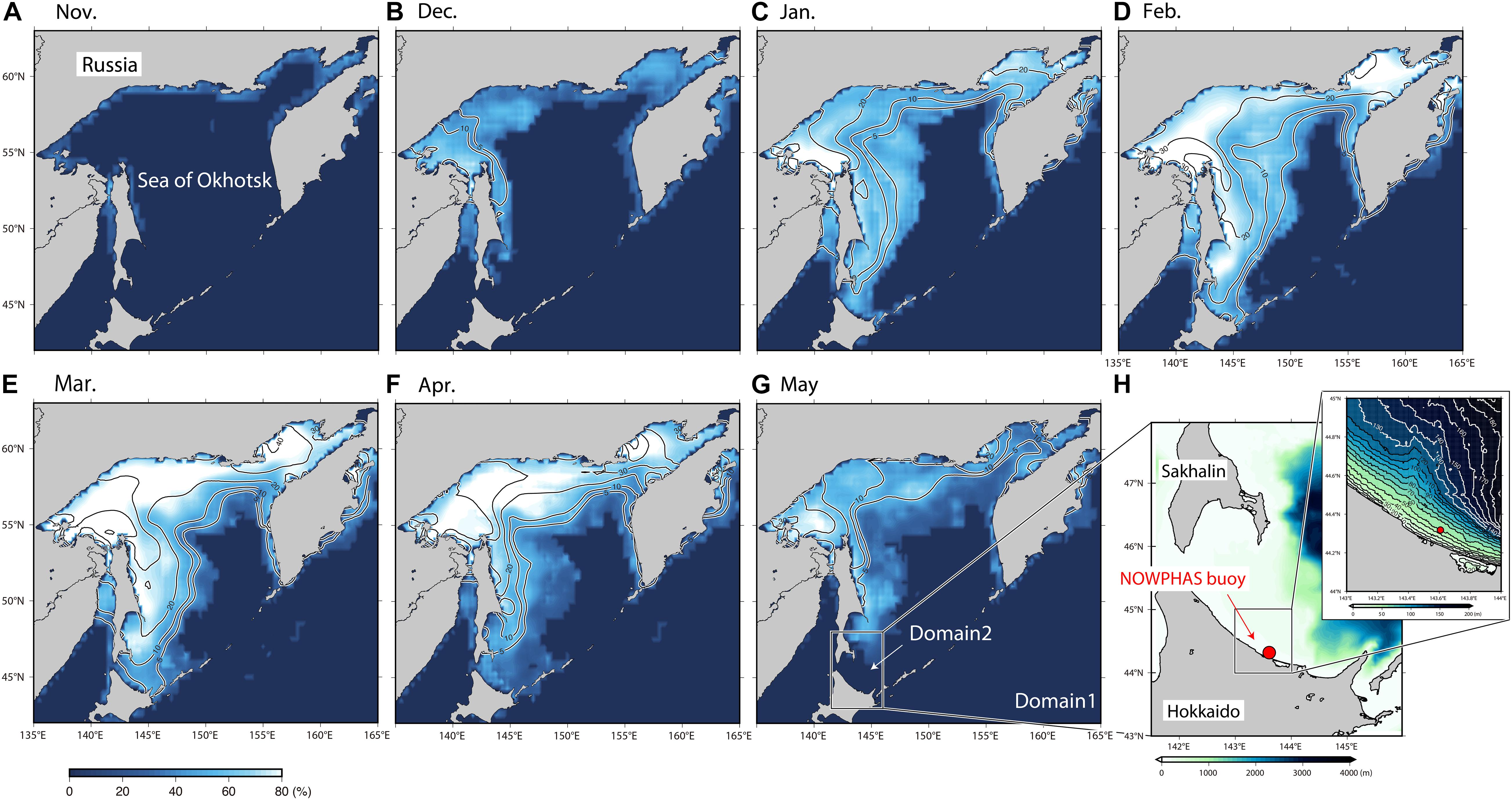
Figure 1. Monthly ice concentration (color) and ice thickness (contour) from November to May during 2008–2010 incorporating two model domains. (A–G) Represent the ice concentration and ice thickness derived from NOAA OI SST V2 and CFSR, respectively. CFSR ice thickness (cm) were smoothed with a two-dimensional boxcar filter with a width of 50 km. (H) Map of the NOWPHAS buoy location (red dot) and the GEBCO, 2020 bottom topography (color). The upper right figure is an enlarged image of the buoy location and bottom topography (color with contours).

(Wavewatch III Development Group (WW3DG), 2019), one of the most widely used third-generation spectral wave models based on the radiative transfer equation for global and regional wave forecasts, implements several parameterizations for wave-ice interaction. In deep water, when currents are absent, the evaluation of wind-generated ocean waves is governed by:

where, N = E/σ is the wave action density spectrum, which is a function of the wave number (k) or relative angular frequency (σ = 2πf), direction (θ), space (x, y), and time (t), E is the wave energy spectral density, f is the frequency, and C_g is the group velocity. For the ice-covered region, the source term on the right-hand side of Eq. (1) is defined as follows:

where, S_in is the input term by wind, S_ds is the dissipation term induced by wave breaking, S_nl is the nonlinear interaction term among spectral components, S_ice is the wave-ice interaction term, and C_i is the ice concentration. Both wind input and dissipation terms (S_in and S_ds) are scaled by the open water fraction (1 − C_i), whereas S_ice is scaled by the ice concentration. The effects of ice on ocean waves can be presented as a complex wavenumber k = k_r + ik_i, with the real part k_r representing the physical wave number related to the wave length and propagation speeds, producing effects analogous to shoaling and refraction by bathymetry, and the imaginary part k_i representing the exponential attenuation coefficient k_i = k_i(x, y, t, σ) which depends on the location, time, and radian frequency. k_i is introduced in the WW3 model as:

here, α is the exponential attenuation rate for wave energy, which is twice that of the amplitude (α = 2k_i). The above equation (Eq. 3) is used to calculate the dissipation by ice in WW3, denoted as IC1–5 (except for IC0).

IC0 is based on Tolman (2003) and provides simple energy flux blocking depending on the local ice concentration. Thus, IC0 does not treat the effect as “dissipation” via the S_ice source term. IC1 allows the user to provide an exponential attenuation rate of amplitude that is uniform in the frequency space (Rogers and Orzech, 2013). IC2 assumes dissipation by friction in the boundary layer below the ice cover (Liu and Mollo-Christensen, 1988). IC3 treats the ice cover as a linear viscoelastic layer based on the model by Wang and Shen (2010). IC4 was introduced by Collins and Rogers (2017) and provides the wave energy dissipation by one of several simple, empirical, and parametric forms through direct fitting with field data. IC4 is different from the other models and needs seven empirical formulas denoted as IC4M1–M7. In addition, IC5 uses a viscoelastic model based on Mosig et al. (2015). k_i is implemented for source functions in IC1–5. The estimation of k_r requires IC2, IC3, and IC5 to provide a new dispersion relation. Descriptions of these models are provided in Supplementary Text 1.

WW3 wave–ice parameterization models were applied in several recent studies on field observations from the Arctic Sea, in regions such as the Barents Sea, Chukchi Sea, and Beaufort Sea (e.g., Cheng et al., 2020; Liu et al., 2020; Nose et al., 2020). Nose et al. (2020) evaluated the uncertainty of wave–ice parameterization models, using three theoretical models (IC2, IC3, and IC5) and the field observations obtained during November in the Chukchi Sea. In addition, Liu et al. (2020) validated the performance of three wave–ice parameterization models (IC2, IC3, and IC4M1–M4) using the field observation from April to May in the Barents Sea. The results suggest that IC3 and IC4M2 corroborate the observations the most. Although sea ice is expected to have a significant impact on the wave fields, no studies have evaluated the effect of sea ice on the wave field in the SO. This study evaluates the wave fields derived from six wave–ice parameterization models (IC0–5 in WW3) using the buoy observations on the north coast of Hokkaido (see Figure 1H). In this study, the wave fields derived from the models were also evaluated for both open ocean and ice-covered conditions. Moreover, the impact of sea ice on wave fields using model simulations with and without sea ice was also clarified. This study had two advantages over previous studies. The first is the evaluation of a considerable number of six wave–ice parameterization models. Six empirical models for IC4 (IC4M1–M7 except for IC4M5) were also evaluated in this study. The second advantage is the use of time-rich observation data. The SO exhibits periods of open ocean and ice-covered conditions, and the buoy observation fully covers both periods (3 years in this study). Therefore, considering the accuracy of the modeled wave field, it can be reliably used to compare the open ocean and ice-covered conditions in the same region.

Materials and Methods

Model Design

Two model domains were created using a nesting process for a horizontal resolution of 0.25° (domain 1) and 0.08° (domain 2) (Figure 1G). The outer domain (domain 1) covers the entire SO (42°–63°N, 135°–165°E). The inner domain (domain 2) was used to validate the wave fields in the coastal area (43°–48°N, 141.5°–146°E). The directional resolution was 10°, and the frequency range was 0.035--1.1 Hz, which was logarithmically discretized into 30 increments. GEBCO, 2020² was used to provide the bottom topography and coastlines.

The simulation of domain 1 incorporated 6-hourly surface wind data from the 55-year JMA Reanalysis (JRA55) (Kobayashi et al., 2015). This product is approximately 55 km in latitude and longitude. In addition, the wind data for domain 2 were obtained from the JRA55 dynamic regional downscaling product (DSJRA55) (Kayaba et al., 2016) developed by JMA, which has a spatial resolution of 5 km and a temporal resolution of 1 h. Daily ice concentration was obtained from NOAA Optimum Interpolation (OI) sea surface temperature (SST) version 2 high-resolution dataset with a 0.25° × 0.25° spatial grid (Reynolds et al., 2007). Ice thickness was incorporated from the Climate Forecast System Reanalysis (CFSR) produced by the National Centers for Environmental Prediction (NCEP) (Saha et al., 2010). The CFSR product has a spatial resolution of 0.25° at the equator, extending to a global 0.5° beyond the tropics, with a temporal resolution of 6 h. The wind, ice concentration, and thickness data were linearly interpolated to the same spatial grid in the wave simulation of both domains. On the north coast of Hokkaido, a southeastward Soya warm current exists along the coast throughout the year. However, this study does not include the influence of ocean currents in model simulation because the strength of the ocean current fluctuates seasonally, and is weak during winter (Ohshima et al., 2017) which is the focal season of this study. In addition, the buoy observation is located in deep water (see section “Buoy Observation” for observation depth), and the effect of tides is also not considered for our model simulation.

In this study, six models for S_ice, IC0, IC1, IC2, IC3, IC4, and IC5 were used (see Supplementary Text 1). In addition, in order to investigate the impact of sea ice on the wave field, simulations that did not incorporate ice concentration were conducted. Hereinafter, the model results without ice concentration are denoted as “Non-ICE.” As shown in Supplementary Table 1, the kinematic viscosity (ν) is required for IC2, and the ν and the effective shear modulus (G) are required for IC3 and IC5 as input parameters. Some theoretical ice parameters (ν and G) for the theoretical models (IC2, IC3, and IC5) have been proposed by previous studies (see Supplementary Table 1). In this study, three, four, and two simulation cases were conducted for IC2, IC3, and IC5, respectively, using the theoretical ice parameters summarized in Supplementary Table 1. In addition, various parameters have also been proposed for the binomial fitting of IC4M2 and the step function of IC4M6 based on different observational data (Supplementary Tables 2, 3). Therefore, eight and six simulation cases were performed for IC4M2 and IC4M6, respectively. Although IC4M5 and IC4M6 both provide a step function in the frequency space, IC4M6 has more steps than IC4M5. Therefore, IC4M5 was excluded from validation in this study. A simple diffusive scattering model (denoted as IS1 in WW3) was used for these simulations. Another scattering model (denoted as IS2) was implemented in WW3. However, the difference between the scattering models (i.e., IS1 and IS2) was small compared to the difference between the dissipation models (IC0–IC5) (not shown). For terms S_in and S_ds, we used both ST4 (Ardhuin et al., 2010; Rascle and Ardhuin, 2013) and ST6 (Rogers et al., 2012; Zieger et al., 2015; Liu et al., 2019). In this study, the model results with ST6 are presented in the main text, while the model results with ST4 are presented in Supplementary Material.

All simulations were performed over a 3-year period from 2008 to 2010. The significant wave height (H_s) and mean wave period (T_m01) were both recorded every hour during the computation period. To simplify the notation, T_m01 is denoted as T_m. To obtain the modeled value at the buoy position, we bilinearly interpolated the fields to the buoy position using the surrounding four grid values from domain 2.

Buoy Observation

To validate the model results of the wave field, we used buoy observation data from the Nationwide Ocean Wave Information Network for Ports and Harbors (NOWPHAS)³, provided by the Ports and Harbors Bureau, Ministry of Land, Infrastructure, Transport, and Tourism (MLIT). Significant wave height and mean wave period data obtained every 20 min were used for the observation depth of 52.6 m in the Monbetsu (south) Station (red dot in Figure 1H). The distance from the coast of the buoy is 8,200 m. Buoy data for 3 years, from 2008 to 2010, were used, same as the modeling period. In the present study, the observation data were averaged from 20 min to 1 h and compared with the simulation results. Figure 2 shows the frequency distribution of H_s and T_m observed by the buoy during 2008–2010. The averages for H_s and T_m are 0.83 m and 4.80 s, respectively (gray bars in Figure 2). The total number of hourly observation data points was 24909. In the present study, to evaluate the model simulations for the ice-covered condition, we utilized values only when the ice concentration in the coastal area (44°–46°N, 142.5°–145.5°E) around the buoy was 10% or more. The number of observation data points was 3277 for the ice-covered condition (blue bars in Figure 2). The number of data points for the ice-covered conditions is significantly reduced compared to that for all data but it covers the entire observation area (Figure 2).

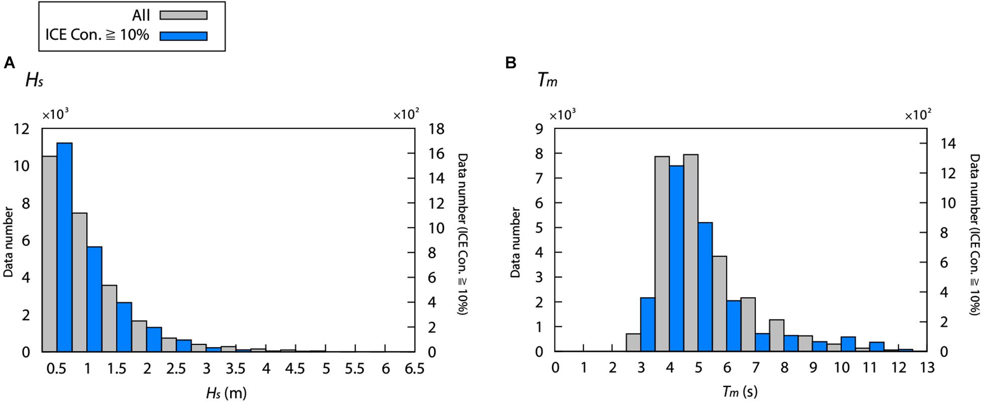
Figure 2. Frequency distribution of hourly (A) H_s and (B) T_m from the NOWPHAS buoy. Gray bars correspond to values for all data during 2008–2010, while blue bars indicate data for the ice- covered condition. Intervals (X–axis) of H_s and T_m are (A) 0.5 m and (B) 1 s, respectively.

The sea ice in the SO is a one-year ice type and is thinner than that of the Arctic Sea (e.g., Nihashi et al., 2018). Although different from the buoy observation points of this study, the floe size of sea ice up to 5 m accounts for 90% of the total in the northeastern coast of Hokkaido (Kioka et al., 2020).

Results

Validation With Buoy

The wave fields for the open water condition were evaluated before comparing them with the wave fields for the ice-covered condition. Figure 3 shows the scatter diagrams for the open water condition for the model simulation and the buoy observation. The bias, RMSE, and correlation coefficient for H_s were 0.02, 0.3, and 0.92 m, and for T_m were 0.14, 0.97, and 0.8 s, respectively. The model results are in close agreement with the buoy observations, and are consistent with the results of a previous study (e.g., Shimura and Mori, 2019). This comparison shows the model results of IC1 because there is no significant difference between the other six models (IC0–5) in the open water condition (not shown). The ST4 model simulation was also calculated with close accuracy to the ST6 model simulation (see Supplementary Figure 1).

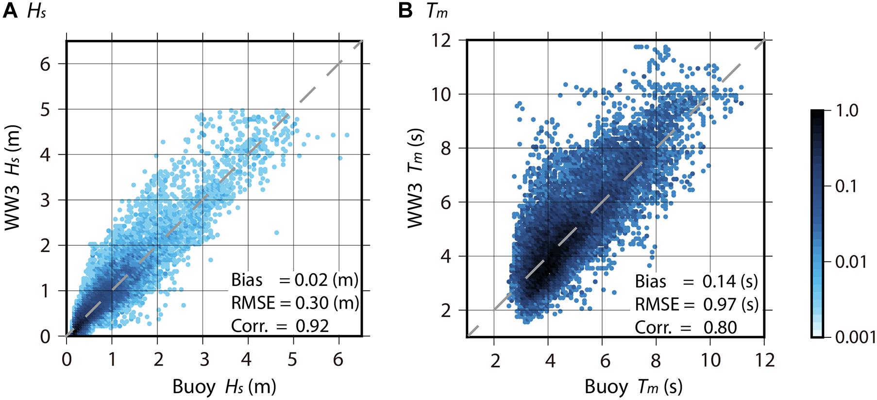
Figure 3. Scatter diagrams of (A) H_s and (B) T_m between the ST6 model simulation (Y–axis) versus buoy observation (X–axis) for the open water condition. Statistical values are shown in the lower left corner of both panels. In this comparison, we used values only when the ice concentration in the coastal area (44°–46°N, 142.5°–145.5°E) around the buoy is 0%. IC1 modeled results are used in this figure. Colored shading indicates normalized data density on a log₁₀-scale. The number of validation data points (hourly) was 19453. The gray broken line y = x is added to both panels.

As shown in Supplementary Tables 1–3, previous studies have proposed various parameters for the three theoretical models (IC2, IC3, and IC5), and two empirical models (IC4M2 and IC4M6). Therefore, these five models are evaluated prior to the comparison between the six wave–ice parameterization models. There are no remarkable differences in IC2 depending on the theoretical parameter, but there are significant differences in IC3 and IC5 (see Supplementary Table 4 for IC2, Supplementary Table 5 for IC3, and Supplementary Table 6 for IC5). Hereafter, IC2 is the simulation result of using ν by Liu et al. (1991), and the results are almost the same (Supplementary Table 4). In addition, IC3 and IC5 are the model results based on ν by Liu et al. (2020) and G by Mosig et al. (2015), and these results demonstrated relatively better accuracy (see Supplementary Tables 5, 6). The empirical parameter of Meylan et al. (2014) was employed for IC4M2 because the model results mostly agree with buoy observations (Supplementary Table 7). The results of IC4M6 are not presented here as it can be almost reproduced by the binomial fitting of IC4M2 (see Supplementary Tables 7, 8).

To visualize the standard deviation (STD), root mean square error (RMSE), and correlation coefficient between the model simulations and NOWPHAS buoy data, Figure 4 displays Taylor diagrams between the two fields (Taylor, 2001). In addition, Table 1 lists the statistical analysis results between the model simulation and buoy observations for H_s and T_m. Additionally, Supplementary Figures 2, 3 display the scatter diagrams for the model simulations and the buoy observations for H_s (T_m). The model accuracies for the ice-covered condition are lower than that for the open water condition except for bias, regardless of the six wave–ice parameterization models (Figures 3, 4 and Table 1). The averaged RMSE and correlation coefficient from all models for the ice-covered condition are 0.44 m and 0.8, for H_s, respectively, and 1.6 s and 0.6, respectively, for T_m, respectively. The RMSE and correlation coefficient of H_s (T_m) for the ice-covered condition are 0.14 m and 0.12 (0.63 s and 0.2) and are less accurate compared with those for the open water condition.

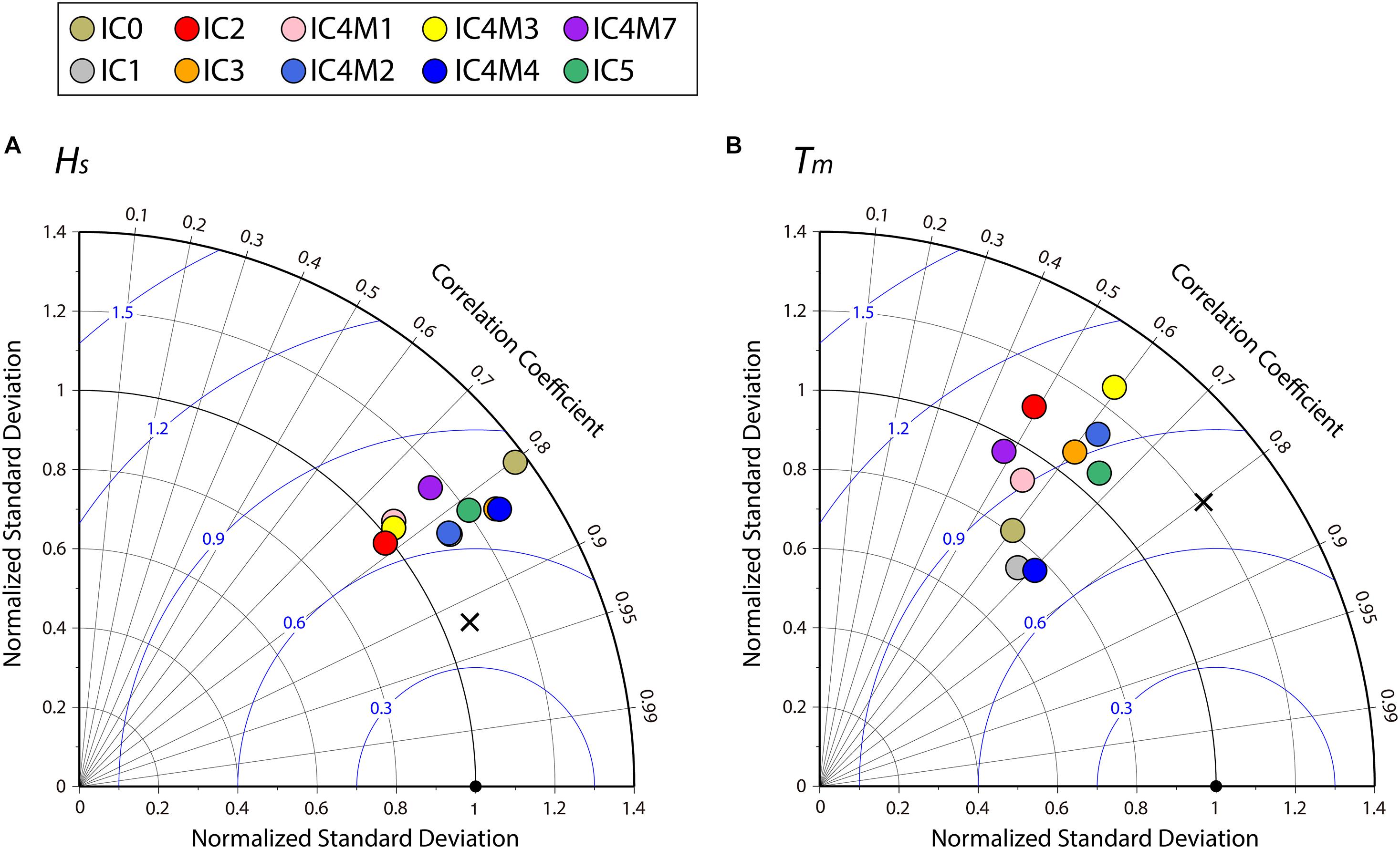
Figure 4. Taylor diagram summarizing the statistical comparison between the NOWPHAS buoy observation and the model simulations with ST6 for the ice-covered condition: (A) H_s and (B) T_m. The number of validation data points is 3277. The source terms of S_ice are represented by the different colored circles (legend in the upper region of the panel). The black cross shows the modeled results of IC1 simulation for the open water condition (i.e., results of Figure 3). The black circle at the bottom indicates the buoy observation. The blue colored contour with an interval of 0.3 denotes the RMSE between the simulations and observations. The RMSE and standard deviations have been normalized by the observed standard deviation. The correlation coefficients between both the fields are shown by the azimuthal position of the simulation field. Note that the position of IC1 (gray circle) overlaps that of IC4M2 (light blue circle) in the left figure.

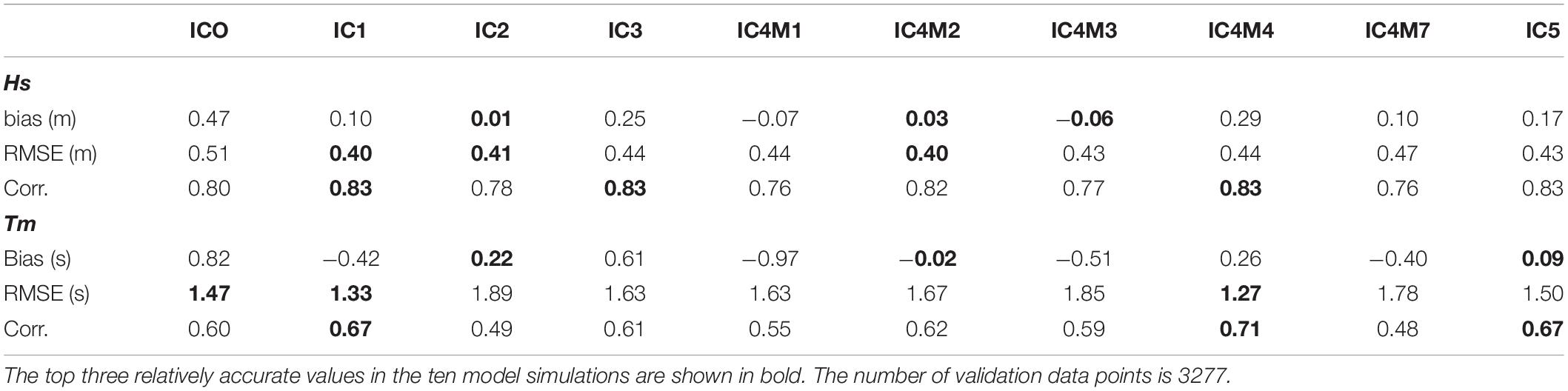
Table 1. Statistical values of H_s and T_m between the ST6 model simulations and buoy observations for the ice-covered condition.

For H_s, all model simulations indicate a correlation coefficient greater than 0.75, a normalized STD between 0.99 and 1.4, and a normalized RMSE (NRMSE) and RMSE of less than 0.83 and 0.52 m, respectively (Figure 4A, Supplementary Figure 2, and Table 1). The bias for all H_s simulation was within ± 0.3 m except for IC0 (Table 1). In particular, the bias of IC2 and IC4M2 were within 0.03 m, which were simulated with high accuracy (Table 1). In addition, the RMSE and the correlation coefficients of IC1 and IC4M2 were 0.4 m and >0.81, respectively, and were better than those of other simulations (Table 1), although the normalized STD of both simulations is slightly overestimated as presented in Figure 4A. In contrast, the bias, NRMSE, and RMSE of IC0 were 0.47, 0.82, and 0.51 m, respectively, and were poorly estimated as compared with other simulations (Figure 4A, Supplementary Figure 2, and Table 1).

Overall, for T_m, all simulations provided corresponding correlation coefficients of less than 0.72, which was relatively worse than those of H_s, same as the open water condition (Figure 4B, Supplementary Figure 3, and Table 1). In addition, the differences in the statistical values between simulations were large compared to those of H_s (Figure 4 and Table 1). IC2, IC4M1, IC4M3, and IC4M7 provided poor simulation results, as their RMSE and correlation coefficients for T_m were greater than 1.62 s and less than 0.6, respectively (Figure 4B, Supplementary Figure 3, and Table 1). In contrast, IC1 and IC4M4 yielded simulations with least amount of error and indicated a NRMSE (RMSE) less than 0.75 (1.34 s) and a correlation coefficient of greater than 0.66, although the normalized STDs for both simulations were less than 0.8 and tend to be underestimated (Figure 4B, Supplementary Figure 3, and Table 1). Moreover, the bias for IC4M2 and IC5 was ± 0.1 s, smaller than those of other simulations (Table 1).

The statistical results, except as shown above for the bias, depend on the averaging interval. Supplementary Table 9 lists the statistical values between the model simulation and buoy observations for the daily mean. The averaged RMSE for H_s and T_m from the all simulations is 0.38 m and 1.24 s, respectively. The correlation coefficient for H_s and T_mis 0.82 and 0.7, respectively. Compared with those for hourly data, the RMSE and correlation coefficient of H_s (T_m) are 0.06 m and 0.02 (0.36 s and 0.1) more accurate, respectively.

Moreover, we validated the model simulations as a function of ice concentration (Figure 5). All H_s simulations were overestimated at low ice concentrations (C_i < 20 %) (Figure 5A). At high ice concentrations (C_i > 20%), the trend was dependent on the simulation (Figure 5A). IC0, IC3, and IC4M4 overestimated, while IC4M1 and IC4M3 tended to underestimate (Figure 5A). IC1 and IC4M2 were relatively close to the buoy observations and were simulated with high accuracy, consistent with the comparison results shown in Figure 4A and Table 1. For T_m, differences between the simulations became remarkable as the ice concentration increased (Figure 5B). IC4M2, IC4M4, and IC5 were in good agreement with the observations (Figure 5B). IC1, IC4M1, IC4M3, and IC4M7 underestimated, especially for IC4M1 and IC4M7 at C_i > 40% (Figure 5B). On the other hand, the T_m of IC0 and IC3 were overestimated, regardless of ice concentration (Figure 5B).

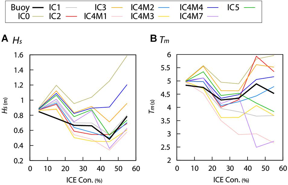
Figure 5. (A) H_s and (B) T_m averaged from the ST6 model simulations and NOWPHAS buoy as a function of ice concentration in 10% bins. The source terms of S_ice are represented by the different colored lines and identified in the legend panel. The horizontal axis denotes the ice concentration in the coastal area around the buoy (44°–46°N, 142.5°–145.5°E).

As described in section “Materials and Methods,” we also evaluated six dissipation models (IC0–IC5) with ST4 (Supplementary Figures 4, 5 and Supplementary Table 10). Overall, there were no significant differences in the wave fields between ST4 and ST6 in the buoy location (Supplementary Figures 4, 5 and Supplementary Table 10). However, the normalized STD for H_s with ST4 was remarkably reduced (approximately 0.15) compared with that of ST6 (Supplementary Figure 4A). When examined as a function of ice concentration, H_s and T_m with ST4 were slightly smaller than those with ST6, but the trend in both simulations remained the same (Supplementary Figure 5).

As shown in Figure 5, the differences between the simulations became significant at high ice concentrations, especially for T_m. Figure 6 and Table 2 show the comparison results between the model simulations and the buoy observations for the high ice-covered condition (ice concentration > 50%). For H_s, IC1 and IC4M2 were relatively agreed with the buoy observations, similar to their comparison results for the ice-covered condition (ice concentration > 10%) shown in Table 1. In addition, the bias, RMSE, and correlation coefficient of IC5 for H_s were – 0.06, 0.35, and 0.91 m, respectively, and were also close to those of IC1 and IC4M2 simulations (Figure 6A and Table 2). For T_m, overall, the qualitative results in Table 2 were similar to the results shown in Table 1, except for quantitative values. IC4M4 results were better than those of other simulations (Table 2). Moreover, IC5 results mostly agree with the observations, compared with the other two theoretical models (IC2 and IC3) (Figure 6B).

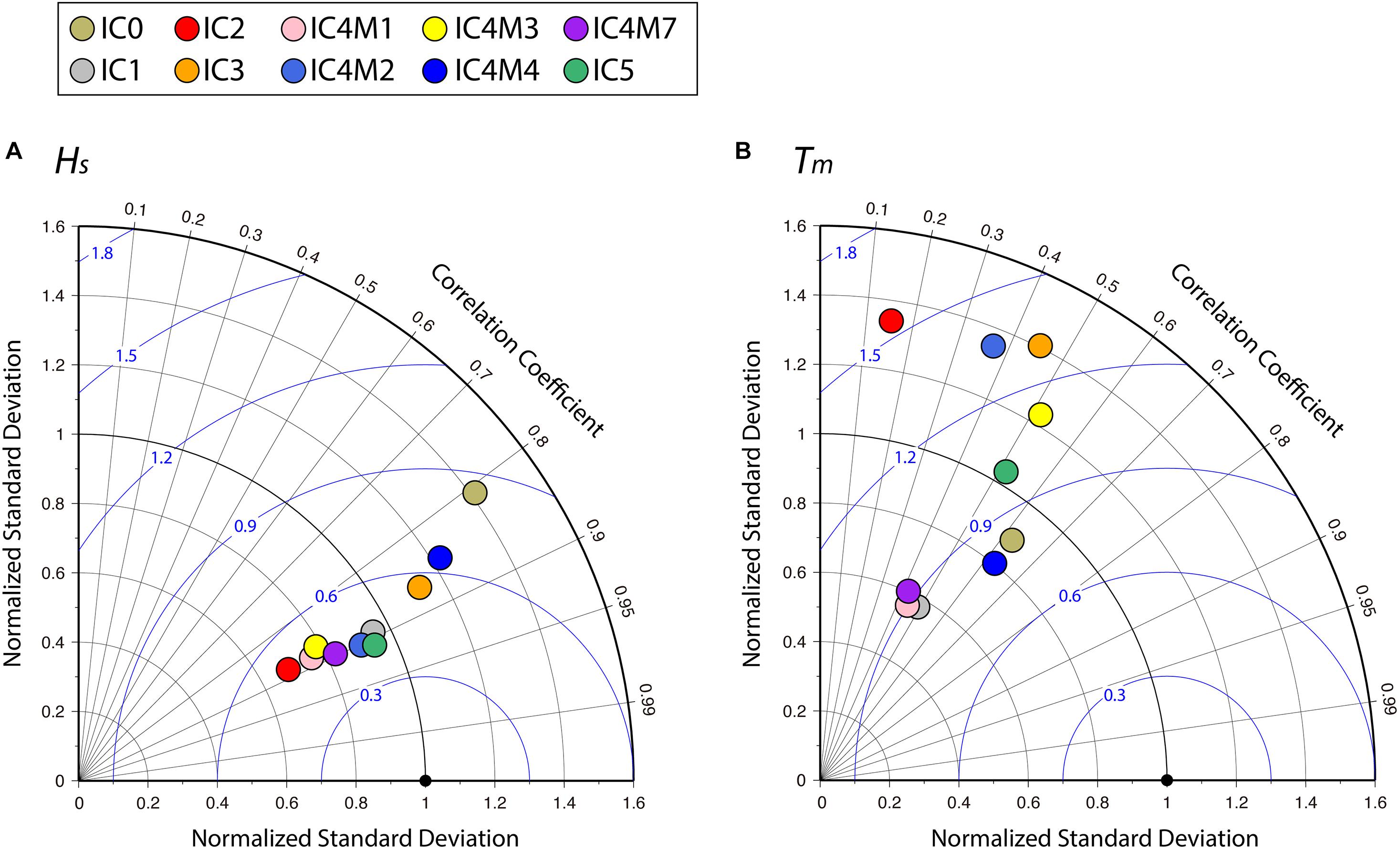
Figure 6. Same as Figure 4 but for high ice-covered condition (ice concentration > 50%): (A) H_s and (B) T_m.

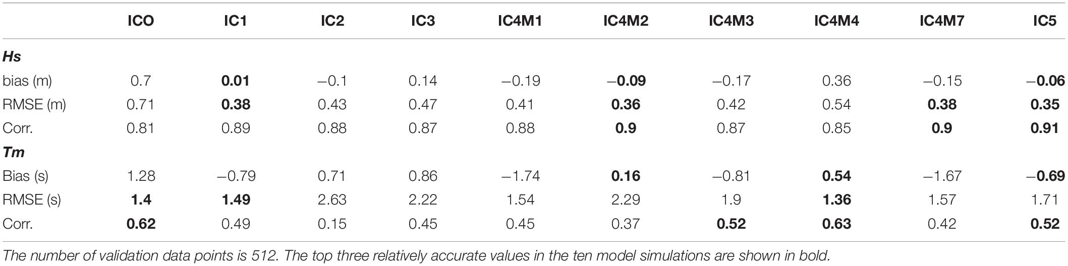
Table 2. Same as Table 1 but for the high ice-covered conditions (ice concentration > 50%).

Sea Ice Impact for Wave Field

To evaluate the impact of sea ice on ocean waves in the SO, we compared the non-ICE simulations and IC4M2, which are relatively accurate, especially in H_s. Figure 7 shows time series and scatter plot of the monthly averaged H_s and T_m for the simulation and observation at the buoy position. In general, large H_s and T_m were observed in the coastal areas of Hokkaido during winter (Figures 7A,B). Interestingly, IC4M2 simulations remarkably mitigated the overestimation of H_s and T_m for non-ICE simulations from January to April, when sea ice existed (i.e., ice concentration is not 0%) (Figures 7A,B). In addition, the improvement of H_s and T_m for IC4M2 is confirmed from the statistical values (Figures 7C,D).

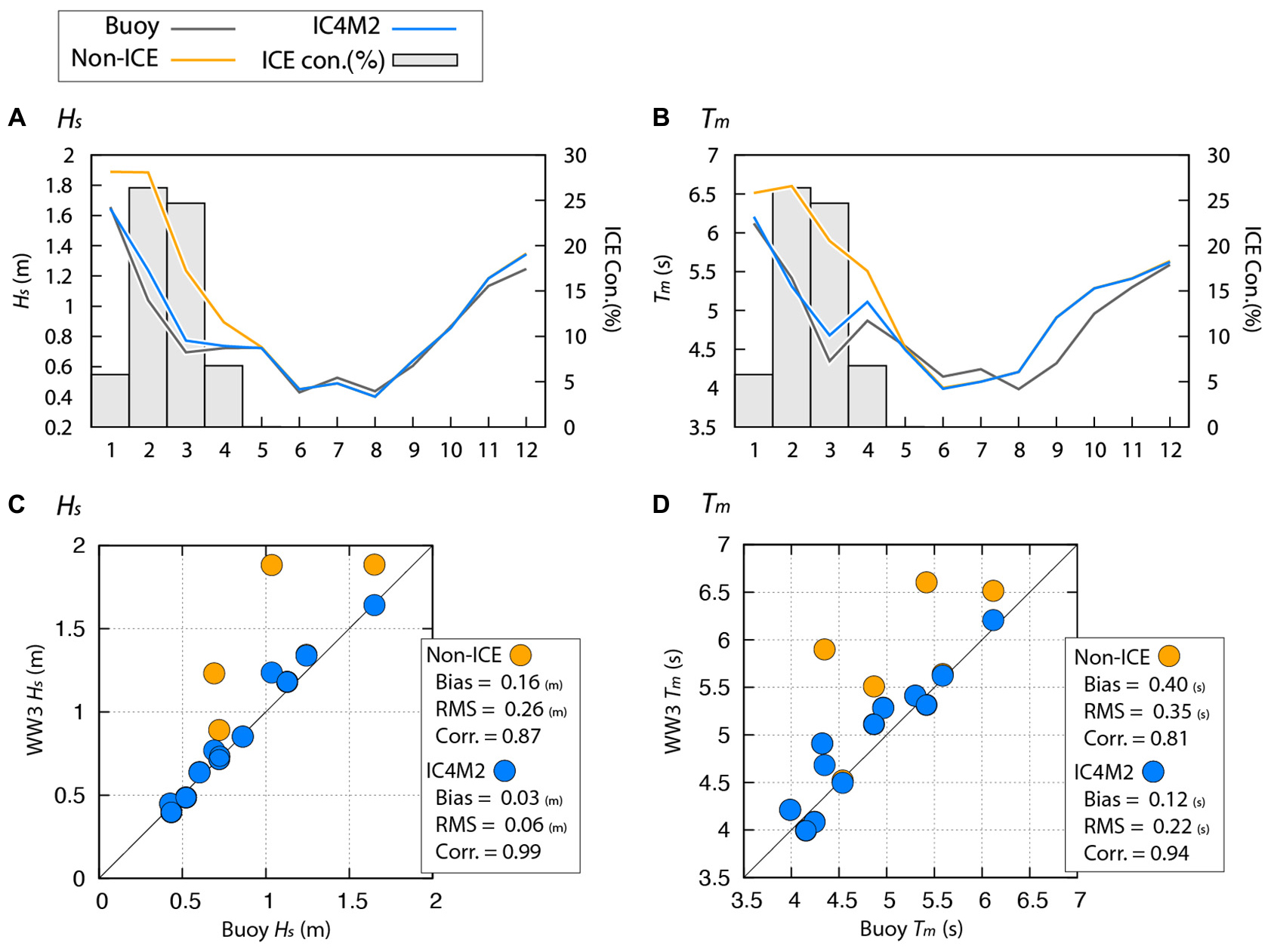
Figure 7. (Upper panels) Temporal variations and (lower panels) scatter plots of monthly averaged (A,C) H_s and (B,D) T_m derived from the simulation and the buoy observation. Both simulations are modeled results with ST6. (A,B) Values are averaged each month from 2008 to 2010. The light gray bars represent the ice concentration in the coastal area around buoy (44°–46°N, 142.5°–145.5°E). (C,D) Statistical values are shown in the lower left corner of both panels. Note that the position of Non-ICE (orange circle) overlaps that of IC4M2 (light blue circle) for the open water condition.

Figure 8 shows the spatial distribution of averaged H_s and T_m in February from IC4M2, and the differences between IC4M2 and non-ICE. As expected, the wave fields were strongly dependent on the sea ice field, and H_s (T_m) became smaller (larger) as the ice concentration increased (Figures 8A,B). The difference in H_s (T_m) between IC4M2 and non-ICE is greater (less) than 1 m (3 s) at high ice concentrations (C_i > 70%) (Figures 8C,D).

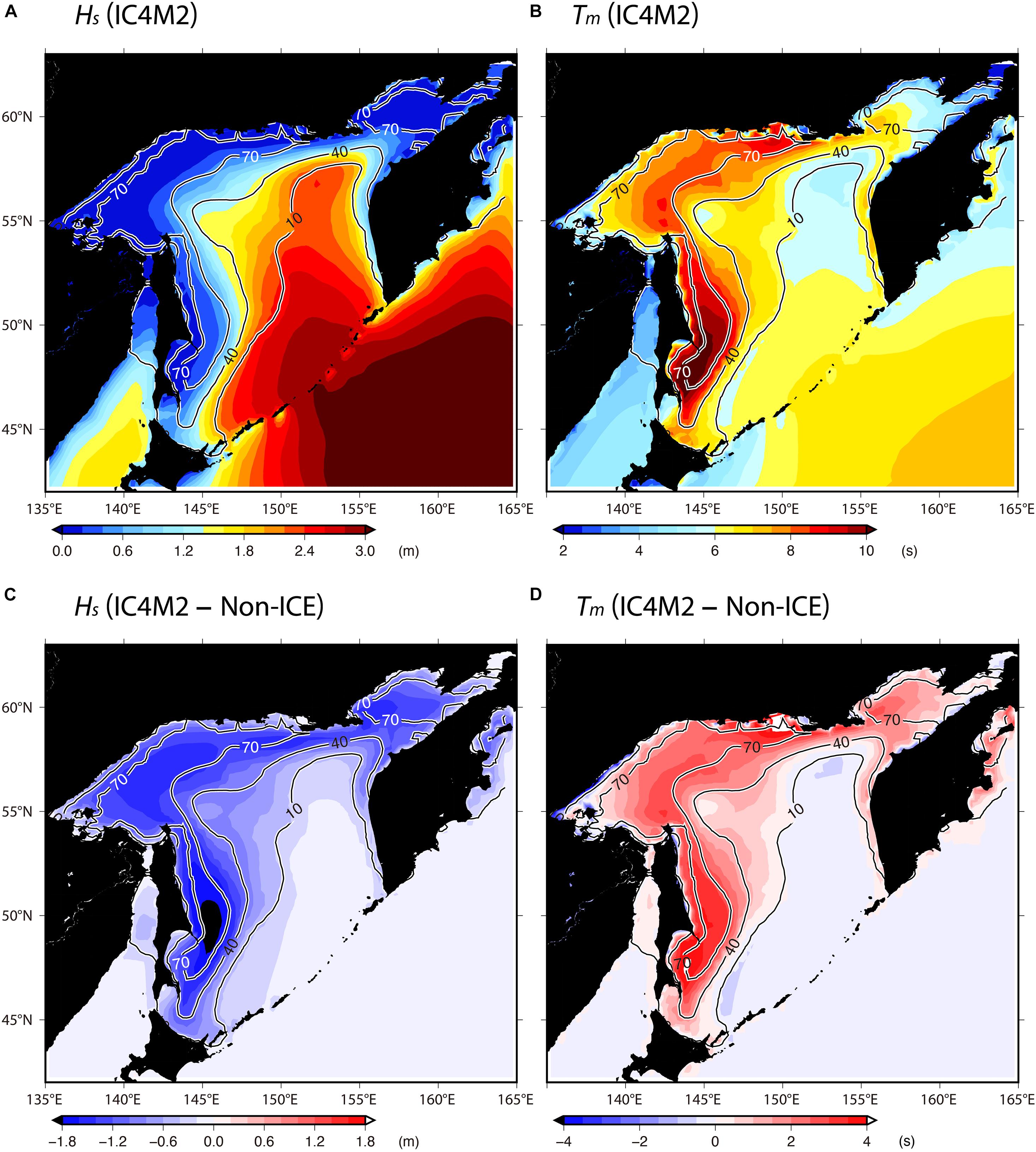
Figure 8. Averaged field (color) of (A) H_s and (B) T_m computed by IC4M2 in February during 2008–2010; difference (color) between IC4M2 and Non-ICE simulations; (C) H_s; (D) T_m. Both simulations are modeled results with ST6. Spatial smoothing using a box filter of horizontal scale 50 km was performed for the ice concentration (contour) (%). In this figure, we used the model results from domain 1.

Discussion

As shown in section “Materials and Methods,” various coefficients have been proposed for the binomial fitting of IC4M2 based on different observational data (Supplementary Table 2). In the eight simulation results of IC4M2, the biases of IC4M6H1, WA3 UK, and WA3 NIWA were greater than 0.15 m (0.43 s) for H_s (T_m) and were larger than the other simulations (Supplementary Table 7). In fact, the attenuation rates of IC4M6H1, WA3 UK, and WA3 NIWA were lower (Supplementary Figure 6). In addition, we validated that the accuracy of IC4M1, IC4M3, and IC4M7 was poor (especially in T_m), and the attenuation rate was significantly different from that of IC4M2 (Supplementary Figure 7). This is probably because the sea ice conditions based on these parameterizations are different from those of the SO. The sea ice thickness is less than 10 cm in the coastal area of Hokkaido (Figure 1). As mentioned in the previous section, 90% of the floe size of sea ice is within 5 m in the coastal area of Hokkaido. In contrast, IC4M1 uses field data with sea ice floe sizes ranging from 20 to 30 m. In addition, IC4M3 is based on an ice thickness between 0.5 and 3 m, which is much thicker than the ice conditions in this study. Moreover, IC4M7 is based on observations of only the pancake ice region, although both pancake and frazil ice may exist in the SO. On the other hand, IC4M2 was in good agreement with observations for H_s, and IC4M4 was relatively close to the observations for T_m. The IC4M2 (i.e., Meylan et al., 2014) and IC4M4 were based on parameterization data from the same field observation in the Antarctic Sea with ice thickness ranging from 0.5 to 1 m; its ice conditions are relatively close to those of SO. The empirical formula of IC4M4 (Kohout et al., 2014) assumes the attenuation is a function of only H_s as shown in Supplementary Text 1. Recently, Kohout et al. (2020) suggested attenuation considers wave period and ice concentration in addition to H_s, based on the observation with < 0.5m ice thickness in the Antarctic Sea. In the future, implementation of this model in WW3 is expected to further improve the accuracy of simulation in thin ice thickness areas such as SO.

Although the simulations of IC5 were relatively worse compared with those of the accurate empirical model (IC4M2 for H_s, and IC4M4 for T_m), IC5 were better than those of two theoretical models (IC2 and IC3), especially for the high ice-covered condition (ice concentration > 50%). The results of these models remarkably depend theoretical parameters (ν for IC2, and ν and G for IC3 and IC5), as shown in Supplementary Tables 4–6 (especially in IC3 and IC5). In this study, constant theoretical parameters were used for IC2, IC3, and IC5. However, these parameters are affected by the ice conditions (e.g., Cheng et al., 2017); thus, these are likely changing both spatially and temporally in the real ocean. Theoretical models have the potential to further improve accuracy in the future, although it is not possible to know the specific types or floe sizes of ice in the entire SO. In other words, the simulation of wave fields under ice-covered conditions depends the accuracy of sea ice used as a model forcing in addition to the accuracy of the model itself, as shown below.

Recently, Nose et al. (2020) revealed that the uncertainty between ice concentration products is greater than the uncertainty between theoretical models (IC2, IC3, and IC5). Thus, it should be noted that our results depend not only on the parameterization for source terms such as S_in, S_ds, and S_ice, but also on the ice concentration used as forcing. In fact, the results of this study are significantly dependent on the temporal resolution of the ice concentration. For example, Figure 9 shows the statistical analysis results for H_s and T_m as functions of the interval of time averaging. As shown in Supplementary Table 9, the NRMS (correlation coefficient) decreases (increases) as the interval of time averaging increases (Figure 9). However, up to approximately 24 h, the rate of change of NRMS and the correlation for both wave fields with the ice condition are larger than those for the open water condition. This is probably due to the daily (24 h) ice concentration used in this study. In addition, the theoretical models IC2, IC3, and IC5 also depend on the ice thickness. Moreover, differences in wind data may also be one cause of uncertainty in wave fields.

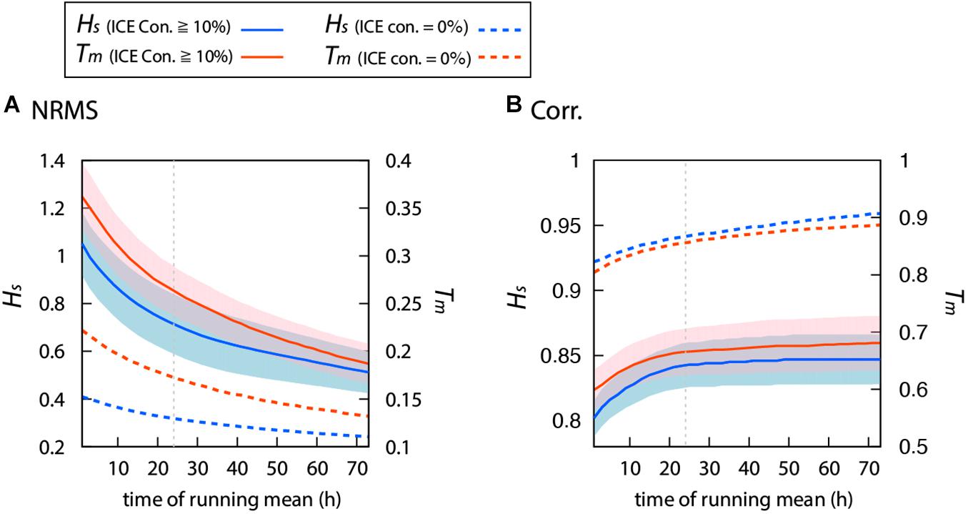
Figure 9. (A) Normalized RMSE and (B) correlation coefficient from ST6 model simulations versus the buoy observation, as a function of time of running mean in 2 h bin. As shown in the legend in the upper corner, solid (broken) lines show the values for the ice-covered condition (open water condition) for H_s (blue) and T_m (red), respectively. In this figure, the normalized RMSE is defined as $\sqrt{\sum {\left(\frac{X_s-X_o-bias}{X_o}\right)}^2}/n$, where X_s is the simulation result, X_o is the observation data, and n is the number of data points. The ice-covered condition result shows the average from all model simulations (i.e., ten modeled results in Figure 4 or Table 1). The color shading indicates the standard deviation of ten modeled simulations. The IC1 simulation result is used for the open water condition. 24 h is highlighted by the gray broken line.

Conclusion

In this study, we evaluated six WW3 wave–ice parameterization models (IC0–IC5) using buoy observations located in the southern part of the Sea of Okhotsk for 3 years from 2008 to 2010. In this comparison, H_s and T_m from the model were evaluated with open ocean and ice-covered conditions. Overall, the accuracy of model results for the ice-covered condition is lower compared to the open water condition, except for the bias. However, in the ice-covered condition, IC4M2 appears to relatively agree with buoy observations for H_s, and IC4M4 is closest to the observations for T_m. We also clarified the impact of sea ice on wave fields in the SO. In the coastal areas, the simulation with sea ice drastically improved the bias of the wave fields (H_s and T_m) compared to that without the simulation without sea ice. In addition, the difference between the simulations with and without sea ice is more than 1 m (3 s) for the monthly mean H_s (T_m). The results of the present study can help researchers and engineers perform calculations of wave fields in the Sea of Okhotsk.

Data Availability Statement

The original contributions presented in the study are included in the article/Supplementary Material, further inquiries can be directed to the corresponding author.

Author Contributions

SI and JO conceived and designed research. SI supervised the work, analyzed the observational data and model simulations, and wrote the manuscript. Both authors contributed to the article and approved the submitted version.

Conflict of Interest

The authors declare that the research was conducted in the absence of any commercial or financial relationships that could be construed as a potential conflict of interest.

Publisher’s Note

All claims expressed in this article are solely those of the authors and do not necessarily represent those of their affiliated organizations, or those of the publisher, the editors and the reviewers. Any product that may be evaluated in this article, or claim that may be made by its manufacturer, is not guaranteed or endorsed by the publisher.

Acknowledgments

We express sincere gratitude to the members of Port and Coastal Research Team, Civil Engineering Research Institute for Cold Region (CERI), Japan, for administrative support. We thank two reviewers for their constructive and fruitful comments.

Supplementary Material

The Supplementary Material for this article can be found online at: https://www.frontiersin.org/articles/10.3389/fmars.2021.713784/full#supplementary-material

Footnotes

1. ^ https://www.data.jma.go.jp/gmd/kaiyou/english/seaice_okhotsk/series_okhotsk_e.html
2. ^ https://www.gebco.net/data_and_products/gridded_bathymetry_data/gebco_2020
3. ^ http://www.mlit.go.jp/kowan/nowphas/index_eng.html

References

Ardhuin, F., Rogers, E., Babanin, A. V., Filipot, J. F., Magne, R., Roland, A., et al. (2010). Semiempirical dissipation source functions for ocean waves. Part I: definition, calibration, and validation. J. Phys. Oceanogr. 40, 1917–1941. doi: 10.1175/2010jpo4324.1
Cheng, S., Rogers, W. E., Thomson, J., Smith, M., Doble, M. J., Wadhams, P., et al. (2017). Calibrating a viscoelastic sea ice model for wave propagation in the arctic fall marginal ice zone. J. Geophys. Res. Oceans 122, 8770–8793. doi: 10.1002/2017JC013275
Cheng, S., Stopa, J., Ardhuin, F., and Shen, H. H. (2020). Spectral attenuation of ocean waves in pack ice and its application in calibrating viscoelastic wave-in-ice models. Crysphere 14, 2053–2069. doi: 10.5194/tc-14-2053-2020
Collins, C. O., and Rogers, W. E. (2017). A Source Term for Wave Attenuation by Sea Ice in WAVEWATCH III, (Technical Memo. NRL/MR7320–17-9726). Washington, D.C: Naval Research Laboratory.
Kayaba, N., Yamada, T., Hayashi, S., Onogi, K., Kobayashi, S., Yoshimoto, K., et al. (2016). Dynamical regional downscaling using the JRA-55 (DSJRA-55). SOLA 12, 1–5. doi: 10.2151/sola.2016-001
Kioka, S., Ishida, M., Hasegawa, T., Takeuchi, T., and Saeki, H. (2020). A study of sea ice floe distribution on Okhotsk sea coast of Hokkaido. Proc. Civ. Eng. Ocean 76, I_905–I_910. doi: 10.2208/jscejoe.76.2_I_905
Kobayashi, S., Ota, Y., Harada, Y., Ebita, A., Moriya, M., Onoda, H., et al. (2015). The JRA-55 reanalysis: general specifications and basic characteristics. J. Meteorol. Soc. Jpn. Ser. II 93, 5–48. doi: 10.2151/jmsj.2015-001
Kohout, A. L., Williams, M. J. M., Dean, S. M., and Meylan, M. H. (2014). Storm-induced sea-ice breakup and the implications for ice extent. Nature 509, 604–607. doi: 10.1038/nature13262
Kohout, A. L., Smith, M., Roach, L. A., Williams, G., Montiel, F., Montiel, F., et al. (2020). Observations of exponential wave attenuation in Antarctic sea ice during the PIPERS campaign. Ann. Glaciol. 61, 196–209. doi: 10.1017/aog.2020.36
Liu, A. K., Holt, B., and Vachon, P. W. (1991). Wave propagation in the marginal ice zone: model predictions and comparisons with buoy and synthetic aperture radar data. J. Geophys. Res. 96, 4605–4621. doi: 10.1029/90JC02267
Liu, A. K., and Mollo-Christensen, E. (1988). Wave propagation in a solid ice pack. J. Phys. Oceanogr. 18, 1702–1712. doi: 10.1175/1520-0485(1988)018<1702:wpiasi>2.0.co;2
Liu, D., Tsarau, A., Guan, C., and Shen, H. H. (2020). Comparison of ice and wind-wave in WAVEWATCH III in the Barents sea. Cold Reg. Sci. Technol. 172:103008. doi: 10.1016/j.coldregions.2020.103008
Liu, Q., Rogers, W. E., Babanin, A. V., Young, I. R., Romero, L., Zieger, S., et al. (2019). Observation-based source terms in the third-generation wave model WAVEWATCH III: updates and verification. J. Phys. Oceanogr. 49, 489–517. doi: 10.1175/jpo-d-18-0137.1
Meylan, M., Bennetts, L. G., and Kohout, A. L. (2014). In situ measurements and analysis of ocean waves in the Antarctic marginal ice zone. Geophys. Res. Lett. 41, 5046–5051. doi: 10.1002/2014GL060809
Mosig, J. E. M., Montiel, F., and Squire, V. A. (2015). Comparison of viscoelastic-type models for ocean wave attenuation in ice-covered seas. J. Geophys. Res. 120, 6072–6090. doi: 10.1002/2015JC010881
Nihashi, S., Kurtz, N. T., Markus, T., Oshima, K., Tateyama, K., and Toyota, T. (2018). Estimation of sea-ice thickness and volume in the Sea of Okhotsk based on ICESat data. Ann. Glaciol. 59, 1–11. doi: 10.1017/aog.2018.8
Nose, T., Waseda, T., Kodaira, T., and Inoue, J. (2020). Satellite-retrieved sea ice concentration uncertainty and its effect on modelling wave evolution in marginal ice zones. Cryosphere 14, 2029–2052. doi: 10.5194/tc-14-2029-2020
Ohshima, K. I., Simizu, D., Ebuchi, N., Morishima, S., and Kashiwase, H. (2017). Volume, heat, and salt transports through the Soya Strait and their seasonal and interannual variations. J. Phys. Oceanogr. 47, 999–1019. doi: 10.1175/jpo-d-16-0210.1
Rascle, N., and Ardhuin, F. (2013). A global wave parameter database for geophysical applications. Part 2: model validation with improved source term parameterization. Ocean Model. 70, 174–188. doi: 10.1016/j.ocemod.2012.12.001
Reynolds, R. W., Smith, T. M., Liu, C., Chelton, D. B., Casey, K. S., and Schlax, M. G. (2007). Daily high-resolution-blended analyses for sea surface temperature. J. Clim. 20, 5473–5496. doi: 10.1175/2007jcli1824.1
Roach, L. A., Bitz, C. M., Horvat, C., and Dean, S. M. (2019). Advances in modeling interactions between sea ice and ocean surface waves. J. Adv. Model. Earth Syst. 11, 4167–4181. doi: 10.1029/2019MS001836
Rogers, W. E., Babanin, A. V., and Wang, D. W. (2012). Observation consistent input and whitecapping dissipation in a model for wind-generated surface waves: description and simple calculations. J. Atmos. Ocean Technol. 29, 1329–1346. doi: 10.1175/JTECH-D-11-00092.1
Rogers, W. E., and Orzech, M. D. (2013). Implementation and Testing of Ice and Mud Source Functions in WAVEWATCH III, (Technical Memo. NRL/MR7320–09-9193). Washington, D.C: Naval Research Laboratory.
Saha, S., Moorthi, S., Pan, H. L., Wu, X., Wang, J., Nadiga, S., et al. (2010). The NCEP climate forecast system reanalysis. Bull. Am. Meteorol. Soc. 91, 1015–1058.
Shimura, T., and Mori, N. (2019). High-resolution wave climate hindcast around Japan and its spectral representation. Coast. Eng. 151, 1–9. doi: 10.1016/j.coastaleng.2019.04.013
Squire, V. A. (2020). Ocean wave interactions with sea ice: a reappraisal. Annu. Rev. Fluid Mech. 52, 37–60. doi: 10.1146/annurev-fluid-010719-060301
Taylor, K. E. (2001). Summarizing multiple aspects of model performance in a single diagram. J. Geophys. Res. 106, 7183–7192. doi: 10.1029/2000JD900719
Tolman, H. L. (2003). Treatment of unresolved islands and ice in wind wave models. Ocean Model. 5, 219–231. doi: 10.1016/S1463-5003(02)00040-9
Wang, R., and Shen, H. H. (2010). Gravity waves propagation into an ice-covered ocean: a viscoelastic model. J. Geophys. Res. 115:C06024. doi: 10.1029/2009JC005591
Wavewatch III Development Group (WW3DG) (2019). User Manual and System Documentation of WAVEWATCH III Version 6.07, Technical Note 333, NOAA/NWS/NCEP/MMAB. College Park, MD: WW3DG, 465.
Keywords: ocean surface waves, sea ice, Sea of Okhotsk, wave model, WAVEWATCH III
Citation: Iwasaki S and Otsuka J (2021) Evaluation of Wave-Ice Parameterization Models in WAVEWATCH III® Along the Coastal Area of the Sea of Okhotsk During Winter. Front. Mar. Sci. 8:713784. doi: 10.3389/fmars.2021.713784
Received: 24 May 2021; Accepted: 12 July 2021;
Published: 06 August 2021.
Edited by:
Giovanni Besio, University of Genoa, ItalyReviewed by:
Matjaz Licer, National Institute of Biology (NIB), SloveniaHajime Mase, Kyoto University, Japan
Copyright © 2021 Iwasaki and Otsuka. This is an open-access article distributed under the terms of the Creative Commons Attribution License (CC BY). The use, distribution or reproduction in other forums is permitted, provided the original author(s) and the copyright owner(s) are credited and that the original publication in this journal is cited, in accordance with accepted academic practice. No use, distribution or reproduction is permitted which does not comply with these terms.
*Correspondence: Shinsuke Iwasaki, iwasaki-s@ceri.go.jp