Uncertainties of Collapse Susceptibility Prediction Based on Remote Sensing and GIS: Effects of Different Machine Learning Models

Introduction

Mountain collapse is a geological phenomenon in which the rock and soil mass on a steep slope suddenly breaks away from the parent body under the action of gravity (Martínez-Moreno et al., 2016; Sun et al., 2017; Yang et al., 2020c). Collapse is a destructive type of geological disaster in human society that directly endangers people’s lives and properties and causes serious environmental problems (Martínez-Moreno et al., 2016; Dou et al., 2020; Yang et al., 2021).

Collapse susceptibility prediction (CSP) and mapping can accurately locate potential areas of collapse occurrence and lay a solid foundation for collapse hazard and risk assessment (Yilmaz et al., 2013). Collapse susceptibility refers to the spatial probability of regional collapse occurrence. In recent years, great progress has been made in mapping collapse susceptibility based on geographic information system (GIS) (Li W et al., 2020; Sun et al., 2021) and quantitative CSP models (Bragagnolo et al., 2020). However, many problems still need to be solved in this research subject. Hence, this article attempts to explore the problems existing in CSP and tries to put forward solutions for promoting the in-depth research of CSP modeling (Merghadi et al., 2020).

A prediction model can be established by analyzing past collapses and their related environmental factors to predict the spatial position of possible collapses in the future (Zhu et al., 2020). The selection of environmental factors, the realization of the connection between collapse and environmental factors, and the selection of an appropriate prediction model are three basic research topics in collapse susceptibility modeling (Shirzadi et al., 2017; Huang et al., 2020a). Some literature works show that environmental factors related to collapse in a large area mainly include topographic and geomorphic factors, land cover factors, and hydrologic environment and lithology factors (Martínez-Moreno et al., 2016; Santo et al., 2017). The specific types of collapse environmental factors can be determined by reviewing the relevant literature, how easy it is to obtain these environmental factors, and the basic evolution characteristics of collapses in the study area (Sun et al., 2017). In the next step, nonlinear connections are made between the collapses and the abovementioned environmental factors, and the results of the connections are used as the input variables of the CSP models (Gutiérrez et al., 2021). At present, the frequency ratio coefficient (Li et al., 2017) and information entropy (Feng and Gong 2020) are commonly used to reflect the above correlation features, among which the frequency ratio coefficient is widely used because of its simple principles and excellent effects (Wang et al., 2016).

Generally, quantitative CSP models can be divided into data-driven models (Hong et al., 2017) and deterministic models (Yang et al., 2020b; Huang D et al., 2020). Deterministic models can be considered mechanical models that mainly calculate the stability of collapse (Berhane et al., 2021). However, such models require relatively uniform collapse types, consistent and detailed soil mechanical parameters, and hydrological factors (Wang et al., 2021). Unfortunately, these prerequisites limit the application of deterministic models, especially in a large area (Godt et al., 2008). Data-driven models can be divided into heuristic models, mathematical statistics models (Tang R-X et al., 2020), and machine learning models (Chen and Chen 2021). Relevant studies show that machine learning models have better generalization ability and susceptibility prediction effects (Rahmati et al., 2019) than heuristic and mathematical statistical models (Hodasová and Bednarik 2021). Machine learning can handle nonlinear corrections between the collapse susceptibility index (output variables) and input variables, and automatically determine the model parameters (Shirzadi et al., 2017; Huang et al., 2020a; Chang et al., 2020).

In recent years, the accuracy of susceptibility models is evolving rapidly from opinion-driven models and mathematical statistical models toward increased uses of machine learning models for the landslide, flood, and other disasters’ susceptibility prediction (Costache 2019; Khosravi et al., 2019; Romali and Yusop 2021). The research studies including background information on their operation, implementation, and performance on machine learning in disaster susceptibility mapping (Chang et al., 2020), such as logistic regression (LR) (Sun et al., 2021), radial basis function network (RBF) (Pham et al., 2016), chi-square automatic interaction detector decision tree (CHAID) (Chen et al., 2017; Park et al., 2018), multi-criteria approach (Mahmoud and Gan 2018), fuzzy logic (Xia et al., 2020), artificial neural network (Bui et al., 2020; Huang et al., 2020d), random forest (RF) (Trigila et al., 2015; Chen et al., 2018), multilayer perceptron (MLP) (Pham et al., 2016; Huang et al., 2020b), support vector machine (SVM) (Zhang et al., 2021), and Bayesian algorithm models (He et al., 2019), have been published.

However, comparisons of current machine learning models for CSP studies are currently lacking; there is no consensus on which model is the most suitable for CSP modeling, and the CSP results of different machine learning models vary greatly (Wang et al., 2014). Hence, it is significant to compare the uncertainty characteristics of CSP modeling by different machine learning models. Furthermore, even if there is no significant difference in the accuracy of CSP results, only a small increase will have an important impact on the distribution rules of collapse susceptibility indexes (CSIs) and change the classification results of susceptibility levels. In addition, due to the influences of environmental factors and machine learning modeling processes, CSP results are often characterized by strong uncertainties. Unfortunately, the existing studies pay little attention to the uncertainties studied under different machine learning models (Feizizadeh et al., 2014). As a whole, in addition to the accuracy analysis of CSP, if some other uncertainty characteristics of CSP results are further analyzed, the CSP effects and feasibility can be better understood (Liu et al., 2020).

To summarize, to explore the uncertainty characteristics of different machine learning models in CSP, six kinds of typical machine learning models, including LR, RBF, MLP, SVM, CHAID, and RF models, are adopted to predict the collapse susceptibility in An’yuan County of China. In order to avoid the uncertainty generated by different study areas, Huichang County of Jiangxi Province in China is also used as the study area.

Methodologies

The purpose of this study is to explore the uncertainties in CSP under different machine learning conditions. The modeling steps of this study are shown in Figure 1 as follows: 1) A spatial dataset is collected using GIS and remote sensing technologies, including 108 collapses and 11 environmental factors (such as the digital elevation model (DEM), normalized difference vegetation index (NDVI), normalized difference built-up index (NDBI), and modified normalized difference water index (MNDWI)). 2) Next, the nonlinear correlations between these collapses and environmental factors are calculated by the FR method in ARCGIS using spatial analysis functions. 3) Collinearity diagnosis of environmental factors and analysis of their relative importance are performed. 4) LR, RBF, MLP, SVM, CHAID, and RF models are used for collapse susceptibility modeling and mapping. 5) The area under the ROC curve (AUC), frequency ratio accuracy (ACC), and other statistical methods are used to evaluate the predictive performance and uncertainty characteristics of the above machine learning models.

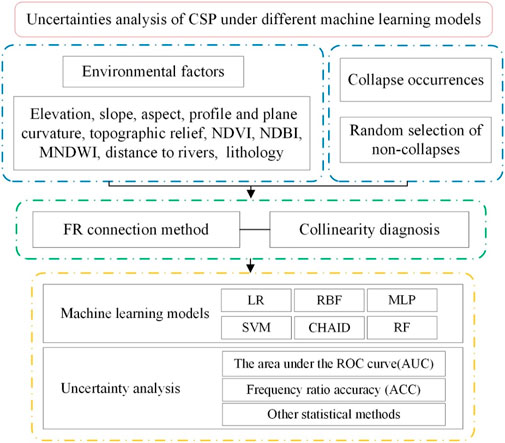
FIGURE 1. Flow chat of regional collapse susceptibility prediction modeling.

Remote Sensing and Geographic Information System for Collapse Susceptibility Prediction

In this study, the collapse-related environmental factors are extracted and managed using RS and GIS technologies, including topographic, land cover, and hydrological and lithological factors. In particular, the topographic factors of elevation, slope, slope aspect, profile and plane curvature, and topographic relief are extracted through the topographic spatial analysis using ArcGIS 10.3 software (Chen and Chen 2021). Meanwhile, the hydrological factors of distance to rivers are extracted through the hydrological analysis tools in GIS. Furthermore, the NDBI, NDVI, and MNDWI are extracted from Landsat TM eight images. In addition, the lithology is drawn and managed in GIS. Finally, the CSMs are produced and displayed by the GIS.

Acquisition of Topographic Factors

The areas with relatively low elevations mainly distributed in the central and northern parts of An’yuan County. The plane and profile curvatures, respectively, describe the vary features of concave and convex terrains from the horizontal and vertical directions (Zheng et al., 2021). Based on the definitions, the plane curvature and profile curvature are, respectively, calculated as the slope of the aspect and the slope of the slope in the ArcGIS 10.3 software. At the same time, the topographic relief reveals the surface relief feature of the study region geography is calculated by the statistical test and the maximum height difference method in GIS (Tang Y et al., 2020).

Analysis of Hydrological Factors

The effects of hydrological factors on collapse occurrences are reflected through the distances of grid units to the river networks. The influence of the river networks on the collapse evolution is mainly due to slope erosion and slope washing, leading to a lower stability of the slope mass (Sun et al., 2021). Furthermore, the distance to rivers shows the balance characteristics among climate, geomorphology, and hydrology.

Acquisitions of Land Cover Factors From RS Images

The NDVI mainly represents the detection of vegetation growth and coverage conditions of the study area (Eq. 1). The NDBI is used to calculate the building distribution features in the study area (Eq. 2). In addition, the MNDWI represents the surface water distribution features (Eq. 3) (Roy et al., 2020). The $P\left(Green\right)$,$P\left(Red\right)$,$P\left(NIR\right)$, and $P\left(MIR\right)$ are the measurements of spectral reflectance obtained in the visible green band, visible red band, near infrared band, and middle infrared band of Landsat eight TM image, respectively (Chang et al., 2020).

Frequency Ratio Analysis

The frequency ratio (FR) is a representation of the importance of attribute intervals of environmental factors to collapse susceptibility (Zhang et al., 2020; Huang et al., 2021). In general, FR > 1 indicates that the attribute interval of the environmental factor has a positive impact on the collapse formation, and FR < 1 indicates that the attribute interval of the environmental factor has a negative impact on the formation of collapse. In this study, the FR of environmental factors is used as the input variable of each model, as shown in Eq. 4, where $N_j$represents the collapse area within the $j$th attribute interval of the environmental factor; $N$represents the total area of collapse in the study area; $S_j$represents the area of the $j$th attribute interval; and $S$ represents the total area of the study area.

Machine Learning Models

Logistic Regression Model

Logistic regression (LR) is a classification and a prediction learning method that approximates the logarithmic probability of real markers with the predicted results of a linear regression model (Chen et al., 2016). For collapse events, the probability of collapse occurrence can be obtained directly by modeling the classification probability without assuming the data distribution in advance. As shown in Eq. 5, $Z$is an effective function of collapse event; $P$is the probability of collapse$P\in \left[\mathrm{0,1}\right]$, where$P/(1-P)$ is the likelihood ratio; $B_0$ is the intercept; $B_i$ is the logistic regression coefficient; and $X_i$ is the collapse environmental factor. In the analysis of collapse susceptibility, LR is used to find the optimal fitting function to describe the relationship between the occurrence of collapses and a set of independent indicators such as the elevation, slope, and formation lithology.

Radial Basis Function Neural Network

Radial basis function (RBF) neural network is a kind of effective multilayer feed forward network with a fast operation speed and strong nonlinear mapping ability (Pham et al., 2018). The input layer is the collapse-related environmental factors represented by$x_i$, information is passed through the input node into the hidden layer without the need for a weight connection. The hidden layer activation function adopts the nonlinear radial basis function, and the Gaussian function is most often used, as shown in Eq. 7:

where $c_i$ indicates the center of the node of the hidden layer and $\sigma$ indicates the control parameter of the kernel functions. The output layer is the linear weighted sum of the output of the hidden functional layer neurons, and the expression is shown in Eq. 8:

Here, $w_{ij}$denotes the connection weights between the hidden layer and the output layer, h denotes the node points of the hidden layer, and n denotes the node points of the output layer. ${\text{y}}_{\text{i}}$ denotes the output of the $j$th node of the network corresponding to the input sample.

Multilayer Perceptron

The multilayered perceptron (MLP) is the most widely used ANN type for classification (Pham et al., 2016). An MLP consists of three main parts: the input layer, hidden layer, and output layer. The FR values of the environmental factors of collapse are the input, and the output layer is the result of the binary variables, where collapse is expressed as 1 and non-collapse is expressed as 0. The classification layer that converts the input variables into output variables is the hidden layer. In this study, the input layer $X_i,i=\mathrm{1,2},\cdots ,11$ is a vector of 11 collapse environmental factors.

The CSP processes of the MLP are as follows: 1) the weight values between the input and the hidden layers are randomly initialized, and the activation function $y=f\left(x\right)$ in the hidden layer is used for the process of passing forward; 2) in the training process of a given network architecture, the network is optimized by adjusting the weight, and the error between the output result and the expected value is calculated; and 3) finally, the connection weights are constantly updated in the iterative processes of error back propagation to obtain a result output with the minimum error, which is regarded as the membership of each terrain unit to the collapse category.

Support Vector Machine

SVM is a typical kind of machine learning (Huang and Zhao 2018). The kernel function is used to map the input vector to a high dimensional feature space so that the nonlinear data can be linearly separable in the high dimensional space. Based on a set of linearly separable training vectors $x_i\left(i=\mathrm{1,2},\cdots ,n\right)$ that includes the FR values of 11 environmental factors and corresponding output classes$y_i=\pm 1$, the collapse classes are distinguished by the maximum clearance of n-dimensional hyperplane. In addition, correct constraints are classified as $y_i((\omega ·x_i)+b)\ge 1$, where $\Vert \omega \Vert$ is the norm of the normal hyper-plane and $b$ is a constant. The Lagrange function is used to solve the convex quadratic optimization problem, as shown in Eq. 9, where${\lambda }_i$is a Lagrange multiplier. For the case of linear inseparability, a relaxation variable ${\xi }_i$is added to control classification errors. The constraints for correct classification are changed as Eq. 10.

Then, $\nu \left(\mathrm{0,1}\right)$ is introduced to consider the wrong classification, and the hyperplane distance is expressed in Eq. 11. The kernel functions of the SVM model include linear, polynomial, radial basis function, and sigmoid; the RBF kernel function is more commonly used for several kinds of landslides and CSP than the others.

Chi-Square Automatic Interactive Detection Decision Tree

The CHAID model has the ability to automatically classify a large number of collapses with environmental factors (Kadavi et al., 2019). After feature selection and data preprocessing, 11 environmental factors are taken as input variables, and “collapse” and “non-collapse” are taken as the output variables in the screening process of the decision tree model. In CHAID, the performance of the classification iteration stops as long as there is no significant chi-square value between the output variable and the environmental factors. Nominal data are used by CHAID as the output variable. If the data are essentially classified, Pearson chi-square, Eq. 12, is used.

Here, $n_{ij}={\displaystyle {\sum }_{n\in D}{f}_n}I\left(|x_n=i\cap y_n=j\right)$, $n_{ij}$indicates the frequency of the unit, $m_{ij}$is the prediction rate of the independent model $\left(x_n=i,y_n=j\right)$, and the corresponding $p=pr(x_d^e>x^2)$.

Random Forest

The RF model is a relatively new and powerful approach to regression and supervised learning that integrates all the results of the classification and regression tree (Emami et al., 2020). RF can alleviate the discontinuities in classification and regression trees and make the predicted values smoother. Classification and regression trees have two disadvantages: first, they are sensitive to training datasets, and different training data may lead to significant changes in the constructed trees; second, a finite number of leaves lead to a limited number of predicted values, thus making the predicted values discontinuous. Fortunately, the RF model can be introduced to effectively overcome these disadvantages (Trigila et al., 2015).

Accuracy Evaluation and Uncertainty Analysis

AUC and ACC of the Model’s Accuracy

The evaluation of CSP model quality is the key to the modeling success. The ROC is a precision evaluation method that does not need to reclassify the CSIs, and the evaluation results are more objective (Cantarino et al., 2019). The area under ROC curve (AUC) is used to evaluate the model accuracy quantitatively, as shown in Eq. 13, where $n_0$ denotes the number of negative samples, $n_1$denotes the number of positive samples, and $r_i$ represents the order of the $i$th negative sample in the entire test sample. The greater the AUC value is, the better prediction performance of the model.

Predictive accuracy (ACC) is also widely used to evaluate the predictive ability of CSP models. ACC is the ratio of correctly predicted collapse and non-collapse grid units, as shown in Eq. 14, where TP (true positive) and TN (true negative) express the number of correctly classified grid units, and FP (false positive) and FN (false negative) express the number of misclassified grid units.

Uncertainty Analysis

The Kendall synergy coefficient test is used to analyze the difference in the distribution of the CSIs of these machine learning models (García-Ruiz et al., 2010). Additionally, the numerical distribution characteristics of the CSIs predicted by the machine learning models are analyzed from the perspective of both the mean value and standard deviation. Finally, the best machine learning model is obtained through a comparative analysis of the model uncertainty. The null hypothesis of the Kendall coefficient test with the coefficient W is that the prediction results of different models are consistent, as shown in Eq. 15, where $m$ is the evaluation model, $n$ is the sample number, $R_i$ is the sum of the rank of the first sample, and $W\in [0,1]$.

When the prediction results of different models are consistent, W is 1. When the W value is less than 1, the Kendall synergy coefficient should reject the null hypothesis (the differences in the prediction results of the original hypothesis are not significant). When the sample size tends to infinity, the significance test can be performed using Eq. 16. At the significance level of 5%, the chi-square test is used to evaluate the significance difference between machine learning model groups. Therefore, if the calculated significance level is less than or equal to 5%, the null hypothesis is rejected, and the performance of the susceptibility model is significantly different, and vice versa.

Study Area and Database

Introduction of the Study Area

This county is located in the hilly southeastern region, Jiangxi Province of China. The latitude and longitude ranges are 115°9′ E ∼ 115°37′ E, 24°52′ N ∼ 25°36′ N, with a total area of 2,374.59 km². Almost 83.43% of the total area is mountainous; the middle part of the terrain rises and slopes to the north and south (Figure 2). The elevation ranges from 180 to 1,150 m, and the slope ranges from 0° to 58.4°. There are many rivers in An’yuan County with rich water resources. The average annual rainfall in the study area has been 1,640 mm from the 1970s to 2020s, and the rainfall is concentrated in April ∼ July. The land use types are mainly forest and bare grassland, and the forest coverage rate of the study area is 71.8%. Geologically, the strata exposed in the study area include pre-Sinian, Sinian, Cambrian, Carboniferous, Jurassic, Cretaceous, and Quaternary strata.

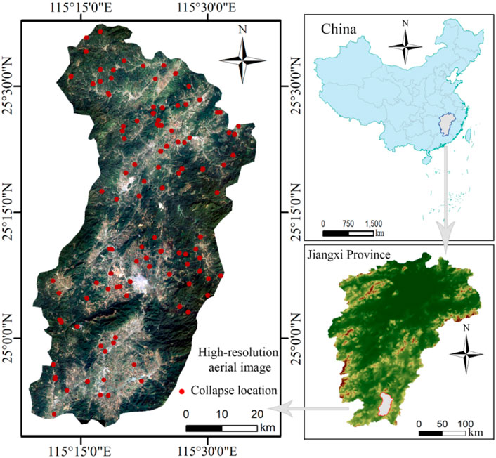
FIGURE 2. Geographical location and collapse data.

Spatial Database

Collapse inventory is the basis for collapse susceptibility mapping. According to the statistics of the collapse inventory of the county natural resources bureau, combining high-resolution remote sensing images and field investigations, a total of 108 collapses (Figure 2) with a density of 4.55 collapses per 100 km⁻² have been identified over approximately 30 years (1978s–2010s). The collapse size of this region is mainly small and medium sized, and the average area is approximately 7,000 m². These collapse disasters have the characteristics of the spatial concentration distribution, and the disaster points are more likely to be distributed near the river network system (Figure 3). Steep landform, rock mass with poor mechanical properties and a complex geological structure are the material basis of collapse evolution. Rainfall, groundwater, earthquakes, and engineering construction are the inducing factors for the formation of collapses (Zheng et al., 2018).

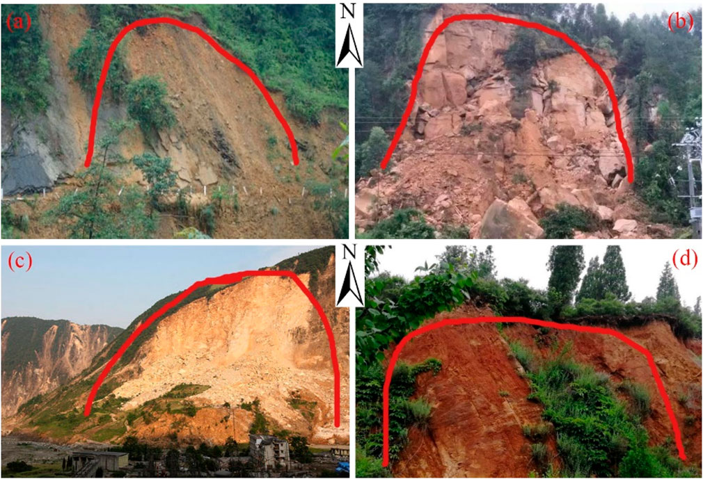
FIGURE 3. Photos of typical collapses in Ganzhou City. (A–D) Examples of four collapses in Ganzhou.

Selection of Collapse Environmental Factors

According to the statistical data and geographical characteristics of An’yuan County, as well as the relevant literature on the selection of collapse-related environmental factors in southeastern China, the types of environmental factors are determined (Yilmaz et al., 2013). In addition, collapse-related environmental factors are specifically acquired based on the data sources of 30 m resolution remote sensing images (Landsat eight TM, October 15, 2013, path/row 121/41 and path/row 121/42), DEMs with a 30 m resolution, and geological maps in GIS (Huang et al., 2020c). As a result, the final 11 environmental factors are topographic factors acquired from DEM data (elevation, slope, topographic relief, profile curvature, etc.), geological factors acquired from a lithology map with a 1:100,000 scale (rock types), hydrological factors (distance to rivers acquired from DEM, and the MNDWI from the above remote sensing image), and land cover (NDVI and NDBI from the above remote sensing image). The collapse inventory and environmental factors are both mapped with a 30 m resolution (Figure 4).

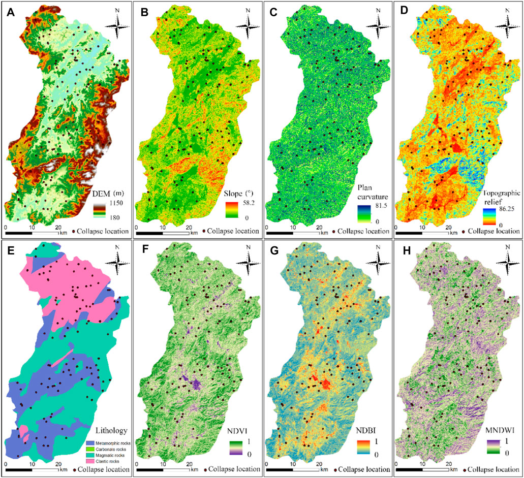
FIGURE 4. Environmental factors (A) elevation; (B) slope; (C) Plan curvature; (D) Topographic relief; (E) lithology; (F) NDVI; (G) NDBI; (H) MNDWI (Aspect, Profile curvature and distance to rivers are not present).

The data types of the environmental factors mainly include continuous and discrete types. In this study, the lithology factor is discrete and divided according to its rock types. The distance to rivers divided into four levels is calculated by the multiloop buffer analysis in ArcGIS 10.2, and the aspect is divided into eight directions as well as flat land. The rest are continuous environmental factors that should be first divided into eight attribute intervals using the natural breaks method according to the literature (Li Y et al., 2020). Then, based on the eight attribute intervals of the environmental factors, the FR method is adopted to quantitatively analyze the relationship between collapses and these environmental factors, as shown in Figure 5.

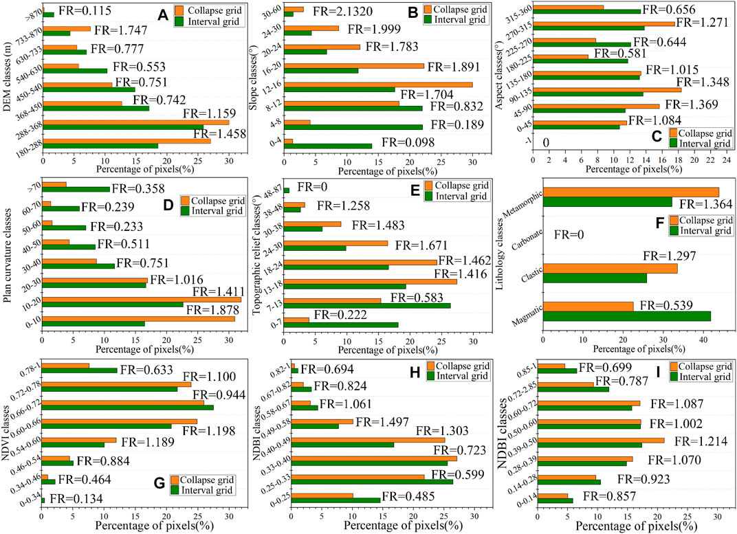
FIGURE 5. Frequency ratio diagram of environmental factors in the An’yuan County: (A) elevation; (B) slope; (C) slope direction; (D) Plane curvature; (E) Topographic relief; (F) lithology; (G) NDVI; (H) NDBI; (I) MNDWI (Profile curvature and distance to rivers are not present).

Analysis of Collapse Affecting Factors

Topographic and Geomorphic Factors

DEM is the data source of other topographic factors, whose effects on collapse are illustrated by taking the elevation and slope as examples. In this study, the collapses are mainly distributed at elevations of 180–368 m with frequency ratios greater than 1 (Figure 5A). The slope has a direct and significant influence on the occurrence of collapses. The collapses are mainly distributed within the slope ranges of [24, 60°] (Figure 4B). The frequency ratios suggest that the slope is one of the most important environmental factors (Figure 5B).

Rock Types

The lithology is the material basis of collapse, influencing the probability of collapse occurrence. As a part of the slope body, different rock types have significant differences in collapse susceptibility (Yang et al., 2020a; Cui et al., 2021). The study area is located in a complex Lingnan structural belt where fold structures and fault structures are developed. The rock types mainly include magmatic rocks (41.83%), metamorphic rocks (32.18%), clastic rocks (25.87%), and carbonate (0.12%) (Figure 4E), with corresponding frequency ratios of 0.539, 1.364, 1.297, and 0, respectively (Figure 5F), showing that metamorphic rocks have greater effects on CSP than others.

Land Cover and Hydrologic Factors

The NDVI and NDBI indirectly reflect the influences of engineering activities on collapses in An’yuan County. The frequency ratio of NDVI is greater than 1 when the NDVI is lower than 0.66 (Figure 4F and Figure 5G). The NDBI with values between 0.49 and 0.71 shows relatively larger frequency ratios (Figure 4G and Figure 5H). For the distance to rivers, the closer the river is to the slope, the higher the soil moisture content of the slope. The area with a distance of less than 300 m to the river system has the highest concentration of collapses (35%), with a frequency ratio of 1.869. Meanwhile, the collapses usually occur under MNDWI ranging from 0.392 to 0.498 with a maximum frequency ratio value of 1.214 (Figure 4H and Figure 5I).

Training and Validation Datasets

A spatial database containing collapse grid cells, non-collapse grid cells, and related environmental factors is required, and these spatial data are further divided into training and test datasets. In this study, a 30 m grid unit is used as the mapping unit; as a result, 108 collapses are divided into 1,463 collapse grid units. Additionally, 1,463 non-collapse grid units are randomly selected from 2,655,972 grid units in the whole study area. The 1,463 collapse grid cells and the same number of non-collapse grid cells are randomly divided into two parts, with a ratio of 70/30 (Zhu et al., 2021). Seventy percent of collapse and non-collapse grid cells are randomly selected for model training, and the rest are used for model testing. The susceptible value of the collapse grid cell is set as 1, while the susceptible value of the non-collapse grid cell is set as 0. Then these values are set as outputs. The calculated FR values of the corresponding environmental factors are set as the inputs of the machine learning. Finally, the trained machine learning is used to predict the CSIs of all grid cells in An’yuan County (Guo et al., 2021).

Mapping of Collapse Susceptibility in An’yuan County

Collinearity Analysis of Environmental Factors

Collinearity among collapse-related environmental factors may decrease the predictive performance and increase the complexity of machine learning modeling. Therefore, in this study, the collinearity of the 11 environmental factors is determined by means of the variance enlargement factor (VIF) and tolerance factor (TOL) before the modeling of the susceptibility, when VIF$\ge$ 5 or TOL $\le$ 0.2, suggesting that the collinearity among environmental factors is so serious that it is necessary to carry out some corresponding data compression processing. As seen from Table 1, the maximum value of VIF is 2.374 and the minimum value of TOL is 0.421, indicating that there is only small multicollinearity among the collapse-related environmental factors; hence, all 11 input factors can be used to predict the collapse susceptibility of the study area.

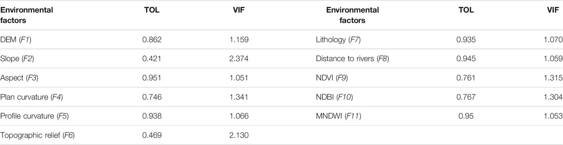
TABLE 1. Collinearity test results of collapse environmental factors.

Collapse Susceptibility Prediction by the Logistic Regression Model

The LR model is trained and tested on the basis of the space dataset, and the regression coefficient ($\beta$), standard errors, and significance of each environmental factor are obtained by the maximum likelihood estimation method (Erener et al., 2016). The calculated CSIs are shown in Eq. 17, and the significances of all variables are less than 0.05, indicating that all variables are statistically significant; the values of the environmental factors are positive, indicating that these environmental factors are conductive to the occurrence of collapses. In the following stages, Eq. 17 shows that the coefficients of the MNDWI, lithology, and slope are 1.389, 1.280, and 1.244, respectively. Hence, these three environmental factors have a greater influence on the collapse prediction than the other factors. The collapse susceptibility of An’yuan County is predicted using Eq. 17 and divided into 5 levels according to the natural break point method, as shown in Figure 5A.

Collapse Susceptibility Prediction by the Radial Basis Function and Multilayered Perceptron Models

The radial basis function (RBF) locally produces an effective nonzero response in a small range and can be used for efficient nonlinear learning. During RBF neural network learning, the number of neurons in the hidden layer is set as 10, and the activation function is the normalized radial basis function. The FR values of the 11 environmental factors are put into the trained model, and the CSIs in the study area are calculated and divided into 5 susceptibility levels, as shown in Figure 6B.

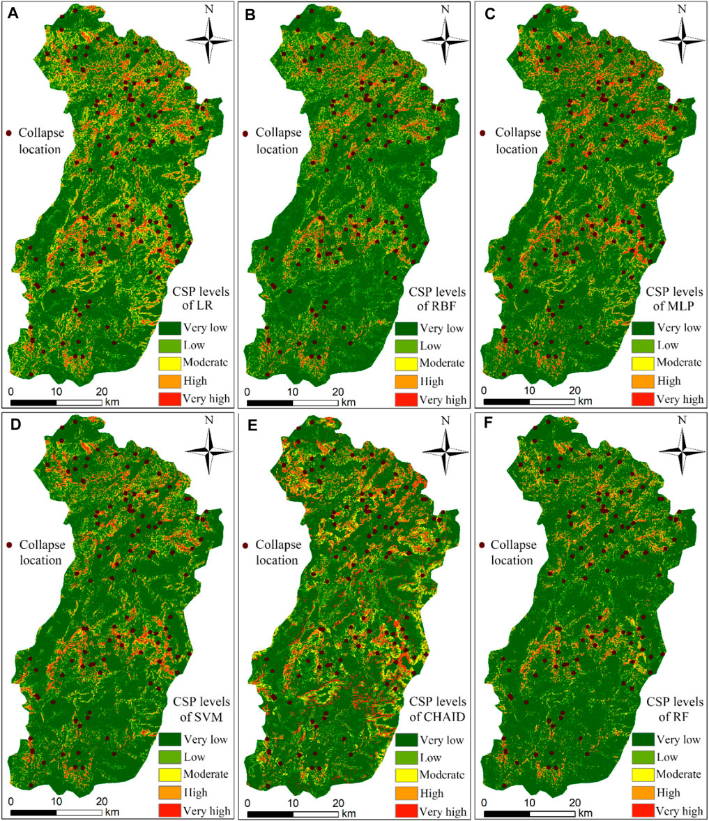
FIGURE 6. CSP levels using machine learning models: (A) LR, (B) RBF, (C) MLP, (D) SVM, (E) CHAID, and (F) RF models.

The two groups of training data of the MLP model are used to build the best model by adjusting the relevant parameters. The learning rate, momentum, and iteration time in the model are 0.01, 0.25, and 500, respectively. Then, the number of hidden layers is set as two, and the activation function is the Softmax function. The trained MLP model is used to predict the CSIs of all the grid units in the whole study area, as shown in Figure 6C.

Collapse Susceptibility Prediction by the Support Vector Machine, CHAID, and RF Models

Based on the SVM for collapse susceptibility modeling, the RBF, which has been widely used, is selected as the kernel function of the SVM. Three parameters, such as regular parameter (C), regression accuracy ($\epsilon$), and kernel parameter ($\gamma$), of the SVM model are determined by the interactive verification method. In this study, the values of C, $\epsilon$, and $\gamma$ are set as 9, 0.1, and 0.6, respectively. The trained SVM is used to map the collapse susceptibility of An’yuan County, as shown in Figure 6D.

The classification significance level of the CHAID prediction results is controlled by the Pearson chi-square statistical test (Althuwaynee et al., 2014). Most of the environmental factors that have strong logical relationships with the instability of collapses are classified by CHAID. The CHAID modeling results show that the occurrence of collapse is most significant for the slope, elevation, lithology, and distance to the river. Finally, the trained CHAID model is used to predict the collapse susceptibility in this county, as shown in Figure 6E.

For the modeling of RF, the out-of-pocket errors of different random forest bags are calculated by R language cyclic iteration. In general, the smaller the out-of-pocket error is, the higher the prediction accuracy of the corresponding model. Loop iteration is carried out in R language; when the number of random features is 4, the out-of-pocket error reaches the minimum. In addition, when the number of classifications is 500, the out-of-pocket error tends to be stable. Hence, the optimal number of random features is set to 4 and the number of decision trees is 500. Finally, the trained RF model is used to obtain the collapse susceptibility, as shown in Figure 6F.

Results and Discussion

Analysis of Collapse Susceptibility Area

Combined with the natural break point method and the distribution trends of the CSIs in An’yuan County, the collapse susceptibility levels (CSLs) are classified into five categories according to equal intervals: very low [0, 0.2], low (0.2, 0.4], moderate (0.4, 0.6], high (0.6, 0.8], and very high (0.8, 1]. Additionally, the CSP accuracy is tested by the collapse point density. The collapse point density of the RF model is 16.87 in the very high CSL, while the collapse point densities of all the other five models are distributed between 4 and 8 (Table 2). Next, the CSL distributions are analyzed as follows:

1) High and very high CSLs are located in the central and northern parts of this county, where the terrain is mainly mountainous and hilly, the river network is dense, erosion of the slope mass by rivers is serious, and engineering activities are intense. The area with very high CSL accounts for about 4% of the total area of this county with a total number of 981 collapse grids. The area with high CSL accounts for approximately 9% of the whole study area with a total of 316 grid units.

2) The area with moderate CSL is located in the low-mountainous and low-altitude areas, with moderate slope and topographic relief, moderate intensity human engineering activities, and distances to the rivers ranging between 300 and 600 m. In this area, the geological conditions are relatively good, and the geological disasters are scattered and distributed. In general, this area accounts for approximately 16% of the total study area with a total number of 122 collapse grid units (Table 2).

3) The areas with low and very low CSLs are mainly located in the southeastern part and the western plains of this county, with gentle slopes, small topographic relief, and intrusive magmatic rocks. In this area, the engineering activities are relatively weak, the distances to rivers are relatively large, and the geological environment conditions are relatively good. As a result, the distribution of collapse disasters is very sparse, with the density of collapse points being less than 0.1 (Table 2).

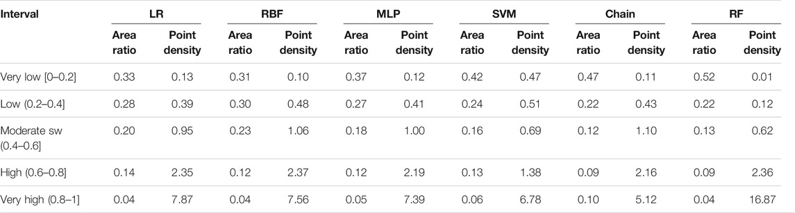
TABLE 2. Prediction effects of each model’s susceptibility interval.

Analysis of the Importance of the Environmental Factors

The importance of environmental factor reflects the contribution of each environmental factor to the collapse susceptibility (Li Y et al., 2020). Due to the uncertainties in machine learning modeling, the importance of collapse-related environmental factors in various machine learning models is different (Figure 7A). This study intends to propose the “weighted mean method” to calculate the importance of each factor based on all the six machine learning models (Tien Bui et al., 2015).

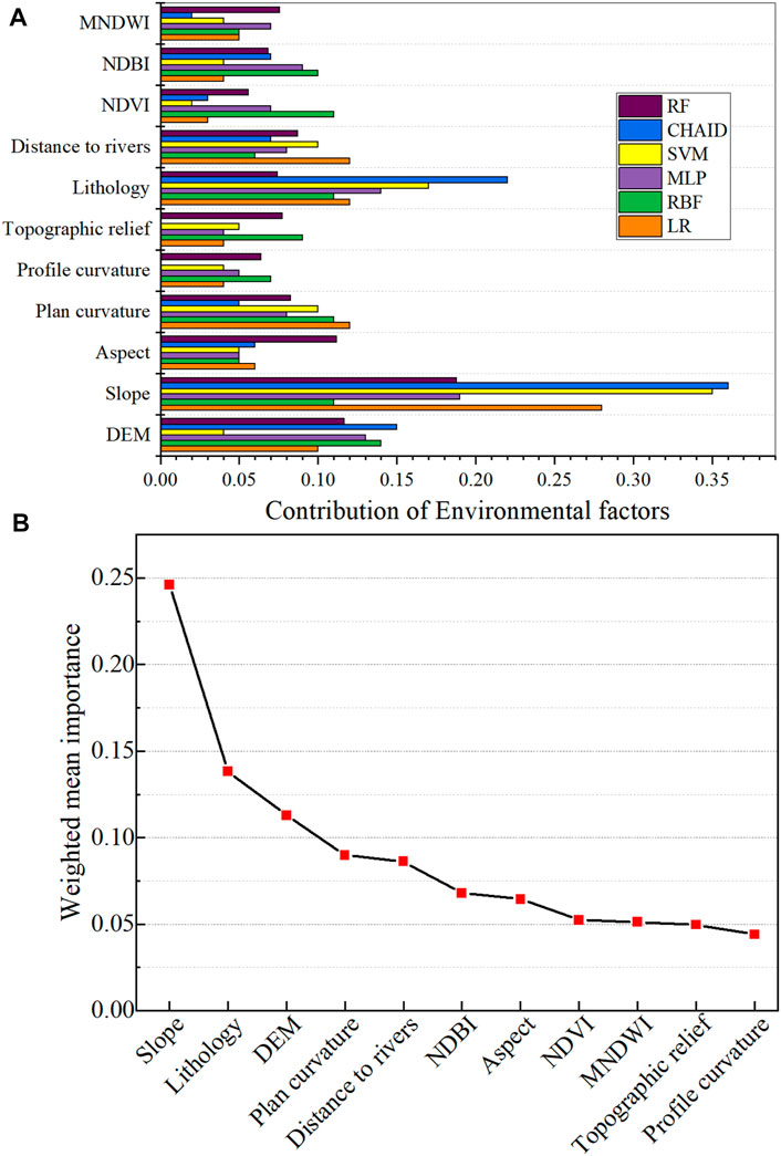
FIGURE 7. Importance of environmental factors. (A) Relative importance of environmental factors in different models. (B) Average importance of environmental factors under different models.

First, the model AUC value is divided by the sum of AUC values in all models, and the calculated ratio value is regarded as the model weight. Second, the model weight is multiplied by the standardized importance of each environmental factor. Third, the multiplied results in the second process are added together to obtain the final importance of each environmental factor. The final importance weights calculated by the “weighted mean method” is shown in Figure 7B, suggesting that among the 11 environmental factors used in this study, the slope (0.25), lithology (0.14), DEM (0.11), and distance to river (0.09) are of higher importance in turn than other factors, while the profile curvature, topographic relief, and MNDWI have the least importance among the six models.

Among them, the mean importance of the slope is the greatest, and collapse tends to occur on slopes greater than 24°. The greater the slope, the more conducive it is to collapse susceptibility. The second important factor is the lithology, the probability of collapse is as high as 43.88% under the conditions of metamorphic rocks, and the probability of collapse of clastic rocks is 33.56%. Following the lithology is the DEM; the collapses mainly occur in the range of 180–368 m, in which the intensity of human engineering activities is relatively high. Although the importance of environmental factors obtained by different models varies in specific values, the weights of environmental factors calculated by the weighted mean method are consistent with different models as a whole.

Validation and Comparison of Model Accuracy

AUC and ACC are both used to evaluate the performance of each machine learning in this county, and the evaluation results are visual and objective. Figure 8 shows that the RF has the highest CSP performance among these machine learning models, with an AUC value of 93.1% and a standard error of 0.005. The CSP performance of CHAID, with an AUC value of 86.2%, is better than those of the other four models, SVM (84.4%), MLP (83.8%), RBF (82.8%), and LR model (82.4%). The comparison results show that the nonlinear relationships between collapse and environmental factors can be more accurately constructed by the RF than the other machine learning.

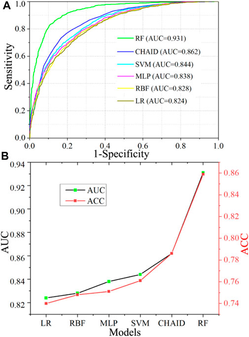
FIGURE 8. Prediction rates of each model performance. (A) AUC values of all models. (B) ACC performance of all models.

According to the ACC prediction accuracies shown in Table 3, the RF model also has the best prediction accuracy, with an ACC value of 85.9%, while those of the other five models are all less than 80%. In general, the accuracy evaluation results of the models based on AUC and ACC are consistent, reflecting the real prediction effect of each machine learning model (Figure 8). Moreover, the literature also shows that RF is an excellent model with good practicability available for landslide and flood disaster susceptibility prediction studies (Trigila et al., 2015; Chen et al., 2018). This is because RF algorithm offers robust performance for accurate CSP with only a small number of adjustments required before training the model.

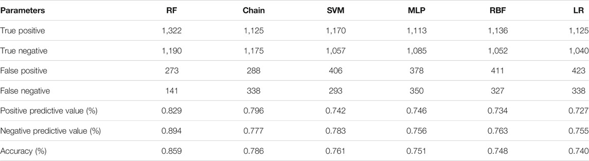
TABLE 3. ACC performance of all models.

Statistical Characteristic Analysis of Collapse Susceptibility Indexes

In the modeling processes of CSP, there are many uncertainties in the selection of environmental factors, correlation analysis between collapse and environmental factors, and different machine learning models for predicting CSIs. In this study, the feasible environmental factor selection scheme and the correlation analysis method are determined by means of a literature review. On these bases, this article focuses on the uncertainty characteristics of different types of machine learning modeling for CSP. The mean value and standard deviation are used to analyze the distribution rules of the predicted CSIs; additionally, the Kendall synergy coefficient method is used to analyze the differences in the distribution trends of the CSIs in various machine learning models at the significance level of 0.05. Finally, the machine learning model with the highest prediction performance and lowest uncertainty is obtained through the comparative analysis.

The Mean and Standard Deviation of the Collapse Susceptibility Indexes

The distribution characteristics of the CSIs predicted by the machine learning models are analyzed from the perspectives of the mean values and standard deviations. According to Figure 9, the mean values of the CSIs of LR, RBF, MLP, SVM, CHAID, and RF are 0.350, 0.345, 0.335, 0.327, 0.321, and 0.272, respectively. These mean values vary between 0.27 and 0.35 and show a gradually decreasing trend from the LR to RF models. In particular, the RF model predicts an average susceptibility index of less than 0.3. The comparison results show that the CSIs of all the machine learning predictors are mainly distributed in the very low and low CSLs, and the number of grid units in the other CSLs decreases gradually. These distribution rules are consistent with the actual collapse probability distribution in An’yuan County because the actual number of collapses in An’yuan County is small and most of the study area is not prone to collapse.

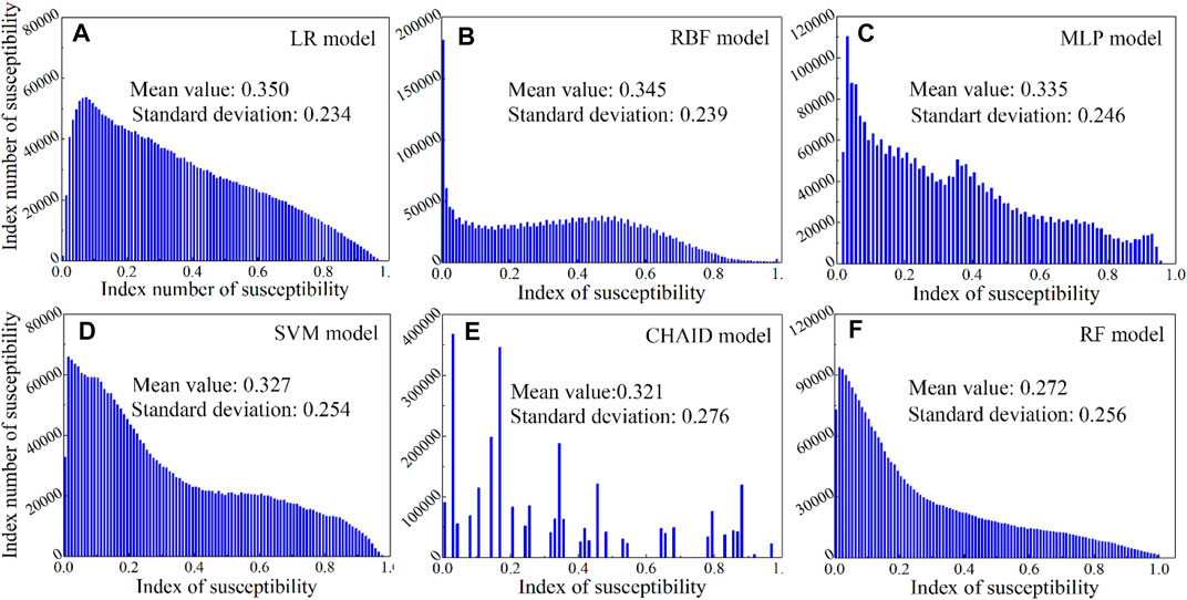
FIGURE 9. Collapse susceptibility indexes distributions of different models: (A) LR model, (B) RBF, (C) MLP, (D) SVM, (E) CHAID, and (F) RF models.

In addition, the standard deviations of the CSIs predicted by all six machine learning models are calculated as LR 0.234, RBF 0.239, MLP 0.246, SVM 0.254, CHAID 0.276, and RF 0.256. The results show that the RF, CHAID, and SVM have greater standard deviations than the other models. A greater standard deviation value means a stronger dispersion of the CSIs, which also means higher recognizability of the collapse probability of different grid cells. Based on the comparisons of the mean values and standard deviations of all the machine learning models, the RF model has the lowest mean value and largest standard deviation, followed by the CHAID, SVM, MLP, RBF, and LR models. Combined with the prediction accuracy of the AUC and ACC of various machine learning models, this suggests that the RF model predicts the collapse susceptibility with the lowest uncertainty, followed by CHAID and SVM models, while the LR model has the highest uncertainty.

Significance Difference Analysis of Collapse Susceptibility Indexes

The Kendall synergy coefficient test is used to evaluate the significant differences between the CSIs predicted by the different machine learning models at the significance level of 5%. The results show that all the p values between the CSIs predicted by the six models are less than 0.05, with a $W$value of 0.062 for Kendall. These p values suggest that there are significant differences between the predicted CSIs of the six machine learning models, and the null hypothesis is rejected. The mean rank values of the LR, RBF, MLP, SVM, CHAID, and RF are 4.06, 3.81, 3.64, 3.48, 3.29, and 2.72, respectively, which are consistent with the prediction performance of these models; the better the prediction performance of the model is, the smaller the mean rank is. For example, the mean rank value of the RF model (2.72) is the best, while that of the LR model (4.06) is relatively poor.

Collapse Susceptibility Prediction of Huichang County for Comparisons

The machine learning models are also undertaking an extensive analysis and comparison using a case study of Huichang County, with 70 collapses (762 grid units) and 11 related environmental factors. In this example, LR, RBF, MLP, SVM, CHAID, and RF models are also used to address the CSP. It can be seen from Figures 10, 11 that RF model achieves excellent results compared to other machine learning models. Furthermore, the uncertainty rule of this example is consistent with those shown in the CSP results of An’yuan County. In detail, the CSP modeling parameters of Huichang County are described as follows.

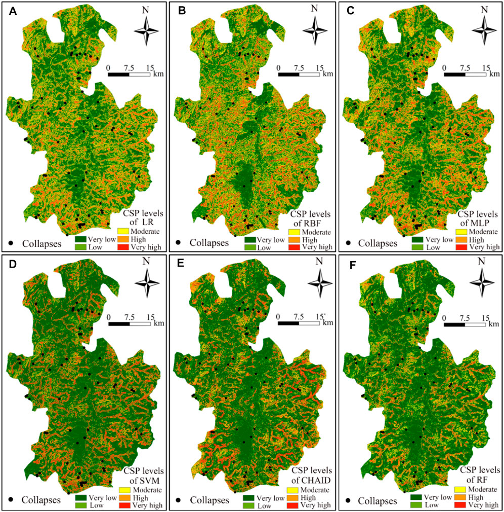
FIGURE 10. Collapse susceptibility graph using machine learning models in Huichang county: (A) LR, (B) RBF, (C) MLP, (D) SVM, (E) CHAID, (F) RF models.

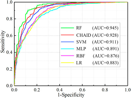
FIGURE 11. AUC values of all machine learning models for CSP in Huichang County.

For the LR model, the absolute values of correlation coefficients of 11 environmental factors are all less than 0.30, and the significances of all input variables are less than 0.05; the values of $\beta$ are positive; here, the coefficients of elevation, slope, distance to rivers, TWI, NDVI, and MNDWI are 1.341, 1.262, 1.643, 1.412, 1.463, and 1.432, respectively. During RBF model learning, the number of neurons in the hidden layer is set as 15, and the activation function is the normalized radial basis function. For the MLP model, its learning rate, momentum, and iteration time are set as 0.01, 0.3, and 2,000, respectively. The number of hidden layers is set as 2, and the activation function is set as the Softmax function. All these three models are built in SPSS 24 software.

For the SVM model, the RBF is widely used as its kernel function in CSP modeling. During the modeling process of SVM, the regular parameter (C), regression accuracy ($\epsilon$), and kernel parameter ($\gamma$) are set as 5, 0.1, and 0.3, respectively. For the CHAID model, its LSP accuracy is estimated by the boosting method, which employs the cross-validation method to boost the accuracy. The rest parameters are the default values, so as to avoid the over-fitting of this model. The SVM and CHAID models for CSP are completed in SPSS Modeler 23. In addition, for the modeling of RF, R language cycle iteration is used to calculate the out-of-pocket errors of different random forests, the optimal number of random features is set to 3, and the number of decision trees is 500.

Future Research Plan

There are many other machine learning models that are not covered in this study or used for comparative analysis (He et al., 2019; Dou et al., 2020). Here, machine learning models adopted in this study are representative to some extent from the current literature, the earliest machine learning (LR, RBF, and MLP methods) and highly popular algorithms such as SVM, CHAID, and RF models (Merghadi et al., 2020). Other machine learning such as deep learning are also worth exploring. Next, the optimal spatial resolutions of collapse inventory and related environmental factors should be determined through some comparative researches of the CSP accuracies at various spatial resolutions. Moreover, more types of collapse-related environmental factors need to be acquired and introduced into the machine learning models, and the optimal combination of environmental factors should be considered. Anyway, various uncertainties characteristics of CSP modeling should be explored in the future research studies.

Conclusion

Based on the collapse inventory and related environmental factors, six machine learning models, namely, the LR, RBF, MLP, SVM, CHAID, and RF, are used to predict the collapse susceptibility in An’yuan County and Huichang County, China. Results show that all of these machine learning models are applicable to the prediction of collapse susceptibility, and their prediction results are consistent overall. The prediction performance of the RF model is 6–10% greater than that of the other five machine learning models.

The contributions of this study can be mainly reflected as follows: 1) Compared with other machine learning models, the RF model has higher CSP accuracy; 2) comparison of the uncertainties of the above models in CSP shows that the RF model has lower uncertainties, followed by the CHAID, SVM, MLP, RBF and LR models; 3) among the above 11 collapse-related environmental factors, the slope has the most important influence on the CSP, followed by the lithology, elevation, and other factors; and 4) the collapses in An’yuan County are concentrated in the areas with very high and high CSLs, specifically for slopes of 24°–60°, elevations of 188–368 m, and a relatively brittle lithology.

Data Availability Statement

The original contributions presented in the study are included in the article/Supplementary Material; further inquiries can be directed to the corresponding author.

Author Contributions

WL was the project manager and wrote the first draft. FH provided Funding acquisition & Supervision. YS prepared the training and test sets and preprocessed Landsat-8 data for CSMs. HH and GS wrote review.

Funding

This research was funded by the National Natural Science Foundation of China (No.41807285), the Natural Science Foundation of Jiangxi Province, China (No. 20192BAB216034), the China Postdoctoral Science Foundation (Nos. 2019M652287 and 2020T130274), and the Jiangxi Provincial Postdoctoral Science Foundation (No. 2019KY08).

Conflict of Interest

The authors declare that the research was conducted in the absence of any commercial or financial relationships that could be construed as a potential conflict of interest.

Publisher’s Note

All claims expressed in this article are solely those of the authors and do not necessarily represent those of their affiliated organizations, or those of the publisher, the editors and the reviewers. Any product that may be evaluated in this article, or claim that may be made by its manufacturer, is not guaranteed or endorsed by the publisher.

References

Althuwaynee, O. F., Pradhan, B., Park, H.-J., and Lee, J. H. (2014). A Novel Ensemble Decision Tree-Based Chi-Squared Automatic Interaction Detection (Chaid) and Multivariate Logistic Regression Models in Landslide Susceptibility Mapping. Landslides 11 (6), 1063–1078. doi:10.1007/s10346-014-0466-0
Berhane, G., Kebede, M., and Alfarrah, N. (2021). Landslide Susceptibility Mapping and Rock Slope Stability Assessment Using Frequency Ratio and Kinematic Analysis in the Mountains of Mgulat Area, Northern ethiopia. Bull. Eng. Geol. Environ. 80 (1), 285–301. doi:10.1007/s10064-020-01905-9
Bragagnolo, L., da Silva, R. V., and Grzybowski, J. M. V. (2020). Landslide Susceptibility Mapping with r.Landslide: A Free Open-Source GIS-Integrated Tool Based on Artificial Neural Networks. Environ. Model. Softw. 123, 104565. doi:10.1016/j.envsoft.2019.104565
Bui, D. T., Tsangaratos, P., Nguyen, V.-T., Liem, N. V., and Trinh, P. T. (2020). Comparing the Prediction Performance of a Deep Learning Neural Network Model with Conventional Machine Learning Models in Landslide Susceptibility Assessment. Catena 188, 104426. doi:10.1016/j.catena.2019.104426
Cantarino, I., Carrion, M. A., Goerlich, F., and Martinez Ibañez, V. (2019). A Roc Analysis-Based Classification Method for Landslide Susceptibility Maps. Landslides 16 (2), 265–282. doi:10.1007/s10346-018-1063-4
Chang, Z., Du, Z., Zhang, F., Huang, F., Chen, J., Li, W., et al. (2020). Landslide Susceptibility Prediction Based on Remote Sensing Images and Gis: Comparisons of Supervised and Unsupervised Machine Learning Models. Remote. Sens. 12 (3), 502. doi:10.3390/rs12030502
Chen, T., Niu, R., and Jia, X. (2016). A Comparison of Information Value and Logistic Regression Models in Landslide Susceptibility Mapping by Using Gis. Environ. Earth Sci. 75 (10), 867. doi:10.1007/s12665-016-5317-y
Chen, W., Xie, X., Peng, J., Shahabi, H., Hong, H., Bui, D. T., et al. (2018). Gis-based Landslide Susceptibility Evaluation Using a Novel Hybrid Integration Approach of Bivariate Statistical Based Random forest Method. Catena 164, 135–149. doi:10.1016/j.catena.2018.01.012
Chen, W., Xie, X., Wang, J., Pradhan, B., Hong, H., Bui, D. T., et al. (2017). A Comparative Study of Logistic Model Tree, Random forest, and Classification and Regression Tree Models for Spatial Prediction of Landslide Susceptibility. Catena 151, 147–160. doi:10.1016/j.catena.2016.11.032
Chen, X., and Chen, W. (2021). Gis-based Landslide Susceptibility Assessment Using Optimized Hybrid Machine Learning Methods. Catena 196, 104833. doi:10.1016/j.catena.2020.104833
Costache, R. (2019). Flood Susceptibility Assessment by Using Bivariate Statistics and Machine Learning Models - A Useful Tool for Flood Risk Management. Water Resour. Manage. 33 (9), 3239–3256. doi:10.1007/s11269-019-02301-z
Cui, Y., Deng, J., Hu, W., Xu, C., Ge, H., Wei, J., et al. (2021). 36cl Exposure Dating of the Mahu Giant Landslide (Sichuan Province, china). Eng. Geology 285, 106039. doi:10.1016/j.enggeo.2021.106039
Dou, J., Yunus, A. P., Bui, D. T., Merghadi, A., Sahana, M., Zhu, Z., et al. (2020). Improved Landslide Assessment Using Support Vector Machine with Bagging, Boosting, and Stacking Ensemble Machine Learning Framework in a Mountainous Watershed, japan. Landslides 17 (3), 641–658. doi:10.1007/s10346-019-01286-5
Emami, S. N., Yousefi, S., Pourghasemi, H. R., Tavangar, S., and Santosh, M. (2020). A Comparative Study on Machine Learning Modeling for Mass Movement Susceptibility Mapping (A Case Study of iran). Bull. Eng. Geol. Environ. 79 (10), 5291–5308. doi:10.1007/s10064-020-01915-7
Erener, A., Mutlu, A., and Sebnem Düzgün, H. (2016). A Comparative Study for Landslide Susceptibility Mapping Using Gis-Based Multi-Criteria Decision Analysis (Mcda), Logistic Regression (Lr) and Association Rule Mining (Arm). Eng. Geology 203, 45–55. doi:10.1016/j.enggeo.2015.09.007
Feizizadeh, B., Jankowski, P., and Blaschke, T. (2014). A Gis Based Spatially-Explicit Sensitivity and Uncertainty Analysis Approach for Multi-Criteria Decision Analysis. Comput. Geosciences. 64, 81–95. doi:10.1016/j.cageo.2013.11.009
Feng, J., and Gong, Z. (2020). Integrated Linguistic Entropy Weight Method and Multi-Objective Programming Model for Supplier Selection and Order Allocation in a Circular Economy: A Case Study. J. Clean. Prod. 277, 122597. doi:10.1016/j.jclepro.2020.122597
García-Ruiz, J. M., Beguería, S., Alatorre, L. C., and Puigdefábregas, J. (2010). Land Cover Changes and Shallow Landsliding in the Flysch Sector of the Spanish Pyrenees. Geomorphology 124 (3-4), 250–259. doi:10.1016/j.geomorph.2010.03.036
Godt, J., Baum, R., Savage, W., Salciarini, D., Schulz, W. H., and Harp, E. L. (2008). Transient Deterministic Shallow Landslide Modeling: Requirements for Susceptibility and hazard Assessments in a Gis Framework. Eng. Geology 102 (3-4), 214–226. doi:10.1016/j.enggeo.2008.03.019
Guo, Z., Shi, Y., Huang, F., Fan, X., and Huang, J. (2021). Landslide Susceptibility Zonation Method Based on c5.0 Decision Tree and K-Means Cluster Algorithms to Improve the Efficiency of Risk Management. Geosci. Front. 12 (6), 101249. doi:10.1016/j.gsf.2021.101249
Gutiérrez, L. F. S., Flores, J. C. M., and Carvajal, H. E. M. (2021). Susceptibility Factors of Drainage Basins to Shallow Landslides in Coffee-Growing Areas in the Department of Caldas, colombia. Environ. Earth Sci. 80 (4), 1–12.
He, Q., Shahabi, H., Shirzadi, A., Li, S., Chen, W., Wang, N., et al. (2019). Landslide Spatial Modelling Using Novel Bivariate Statistical Based Naïve Bayes, RBF Classifier, and RBF Network Machine Learning Algorithms. Sci. total Environ. 663, 1–15. doi:10.1016/j.scitotenv.2019.01.329
Hodasová, K., and Bednarik, M. (2021). Effect of Using Various Weighting Methods in a Process of Landslide Susceptibility Assessment. Nat. Hazards. 105 (1), 481–499. doi:10.1007/s11069-020-04320-1
Hong, H., Chen, W., Xu, C., Youssef, A. M., Pradhan, B., and Bui, D. T. (2017). Rainfall-induced Landslide Susceptibility Assessment at the Chongren Area (china) Using Frequency Ratio, Certainty Factor, and index of Entropy. Geocarto Int. 32 (2), 139–154. doi:10.1080/10106049.2015.1130086
Huang, D., Li, Y. Q., Song, Y. X., Ma, W. Z., and Ma, G. W. (2020). Ejection Landslides Triggered by the 2008 Wenchuan Earthquake and Movement Modelling Using Aerodynamic Theory and Artificial Disintegration Collision Technique. Environ. Earth Sci. 79, 1–23. doi:10.1007/s12665-020-09021-3
Huang, F., Cao, Z., Guo, J., Jiang, S.-H., Li, S., and Guo, Z. (2020a). Comparisons of Heuristic, General Statistical and Machine Learning Models for Landslide Susceptibility Prediction and Mapping. CATENA 191, 104580. doi:10.1016/j.catena.2020.104580
Huang, F., Cao, Z., Jiang, S.-H., Zhou, C., Huang, J., and Guo, Z. (2020b). Landslide Susceptibility Prediction Based on a Semi-supervised Multiple-Layer Perceptron Model. Landslides 17 (12), 2919–2930. doi:10.1007/s10346-020-01473-9
Huang, F., Chen, J., Yao, C., Chang, Z., Jiang, Q., Li, S., et al. (2020c). Susle: A Slope and Seasonal Rainfall-Based Rusle Model for Regional Quantitative Prediction of Soil Erosion. Bull. Eng. Geol. Environ. 79 (10), 5213–5228. doi:10.1007/s10064-020-01886-9
Huang, F., Ye, Z., Jiang, S.-H., Huang, J., Chang, Z., and Chen, J. (2021). Uncertainty Study of Landslide Susceptibility Prediction Considering the Different Attribute Interval Numbers of Environmental Factors and Different Data-Based Models. CATENA 202, 105250. doi:10.1016/j.catena.2021.105250
Huang, F., Zhang, J., Zhou, C., Wang, Y., Huang, J., and Zhu, L. (2020d). A Deep Learning Algorithm Using a Fully Connected Sparse Autoencoder Neural Network for Landslide Susceptibility Prediction. Landslides 17 (1), 217–229. doi:10.1007/s10346-019-01274-9
Huang, Y., and Zhao, L. (2018). Review on Landslide Susceptibility Mapping Using Support Vector Machines. Catena 165, 520–529. doi:10.1016/j.catena.2018.03.003
Kadavi, P. R., Lee, C-W., and Lee, S. (2019). Landslide-susceptibility Mapping in gangwon-Do, south korea, Using Logistic Regression and Decision Tree Models. Environ. earth Sci. 78 (4), 116. doi:10.1007/s12665-019-8119-1
Khosravi, K., Shahabi, H., Pham, B. T., Adamowski, J., Shirzadi, A., Pradhan, B., et al. (2019). A Comparative Assessment of Flood Susceptibility Modeling Using Multi-Criteria Decision-Making Analysis and Machine Learning Methods. J. Hydrol. 573, 311–323. doi:10.1016/j.jhydrol.2019.03.073
Li, L., Lan, H., Guo, C., Zhang, Y., Li, Q., and Wu, Y. (2017). A Modified Frequency Ratio Method for Landslide Susceptibility Assessment. Landslides 14 (2), 727–741. doi:10.1007/s10346-016-0771-x
Li, W., Fan, X., Huang, F., Chen, W., Hong, H., Huang, J., et al. (2020). Uncertainties Analysis of Collapse Susceptibility Prediction Based on Remote Sensing and Gis: Influences of Different Data-Based Models and Connections between Collapses and Environmental Factors. Remote Sens. 12 (24), 4134. Available at: https://www.mdpi.com/2072-4292/12/24/4134. doi:10.3390/rs12244134
Li, Y., Sheng, Y., Chai, B., Zhang, W., Zhang, T., and Wang, J. (2020). Collapse Susceptibility Assessment Using a Support Vector Machine Compared with Back-Propagation and Radial Basis Function Neural Networks. Geomatics, Nat. Hazards Risk. 11 (1), 510–534. doi:10.1080/19475705.2020.1734101
Liu, L.-L., Cheng, Y.-M., Pan, Q.-J., and Dias, D. (2020). Incorporating Stratigraphic Boundary Uncertainty into Reliability Analysis of Slopes in Spatially Variable Soils Using One-Dimensional Conditional Markov Chain Model. Comput. Geotechnics. 118, 103321. doi:10.1016/j.compgeo.2019.103321
Mahmoud, S. H., and Gan, T. Y. (2018). Multi-criteria Approach to Develop Flood Susceptibility Maps in Arid Regions of Middle East. J. Clean. Prod. 196, 216–229. doi:10.1016/j.jclepro.2018.06.047
Martínez-Moreno, F. J., Galindo-Zaldívar, J., González-Castillo, L., and Azañón, J. M. (2016). Collapse Susceptibility Map in Abandoned Mining Areas by Microgravity Survey: A Case Study in Candado hill (Málaga, Southern Spain). J. Appl. Geophys. 130, 101–109. doi:10.1016/j.jappgeo.2016.04.017
Merghadi, A., Yunus, A. P., Dou, J., Whiteley, J., ThaiPham, B., and Avtar, R. (2020). Machine Learning Methods for Landslide Susceptibility Studies: A Comparative Overview of Algorithm Performance. Earth-Science Rev. 207, 103225. doi:10.1016/j.earscirev.2020.103225
Park, S.-J., Lee, C.-W., Lee, S., and Lee, M.-J. (2018). Landslide Susceptibility Mapping and Comparison Using Decision Tree Models: A Case Study of Jumunjin Area, Korea. Remote Sens. 10 (10), 1545. Available at: https://www.mdpi.com/2072-4292/10/10/1545. doi:10.3390/rs10101545
Pham, B. T., Pradhan, B., Tien Bui, D., Prakash, I., and Dholakia, M. B. (2016). A Comparative Study of Different Machine Learning Methods for Landslide Susceptibility Assessment: A Case Study of Uttarakhand Area (india). Environ. Model. Softw. 84, 240–250. doi:10.1016/j.envsoft.2016.07.005
Pham, B. T., Shirzadi, A., Tien Bui, D., Prakash, I., and Dholakia, M. B. (2018). A Hybrid Machine Learning Ensemble Approach Based on a Radial Basis Function Neural Network and Rotation forest for Landslide Susceptibility Modeling: A Case Study in the Himalayan Area, india. Int. J. Sediment Res. 33 (2), 157–170. doi:10.1016/j.ijsrc.2017.09.008
Rahmati, O., Yousefi, S., Kalantari, Z., Uuemaa, E., Teimurian, T., Keesstra, S., et al. (2019). Multi-hazard Exposure Mapping Using Machine Learning Techniques: A Case Study from iran. Remote Sens. 11 (16), 1943. doi:10.3390/rs11161943
Romali, N. S., and Yusop, Z. (2021). Flood Damage and Risk Assessment for Urban Area in malaysia. Hydrol. Res. 52 (1), 142–159. doi:10.2166/nh.2020.121
Roy, P., Chandra Pal, S., Chakrabortty, R., Chowdhuri, I., Malik, S., and Das, B. (2020). Threats of Climate and Land Use Change on Future Flood Susceptibility. J. Clean. Prod. 272, 122757. doi:10.1016/j.jclepro.2020.122757
Santo, A., Budetta, P., Forte, G., Marino, E., and Pignalosa, A. (2017). Karst Collapse Susceptibility Assessment: A Case Study on the Amalfi Coast (Southern italy). Geomorphology 285, 247–259. doi:10.1016/j.geomorph.2017.02.012
Shirzadi, A., Shahabi, H., Chapi, K., Bui, D. T., Pham, B. T., Shahedi, K., et al. (2017). A Comparative Study between Popular Statistical and Machine Learning Methods for Simulating Volume of Landslides. Catena 157, 213–226. doi:10.1016/j.catena.2017.05.016
Sun, D., Xu, J., Wen, H., and Wang, D. (2021). Assessment of Landslide Susceptibility Mapping Based on Bayesian Hyperparameter Optimization: A Comparison between Logistic Regression and Random forest. Eng. Geology 281, 105972. doi:10.1016/j.enggeo.2020.105972
Sun, Q., Tang, Z., and Yuanyao, L. (2017). Susceptibility Assessment of Rock Collapse Hazards in Longjuba Area Based on Dummy Variables Analysis. Hydrogeol. Eng. Geol. 44, 127–135.
Tang, R-X., Kulatilake, P. H., Yan, E-C., and Cai, J. S. (2020). Evaluating Landslide Susceptibility Based on Cluster Analysis, Probabilistic Methods, and Artificial Neural Networks. Bull. Eng. Geology. Environ. 79 (5), 2235–2254. doi:10.1007/s10064-019-01684-y
Tang, Y., Feng, F., Guo, Z., Feng, W., Li, Z., Wang, J., et al. (2020). Integrating Principal Component Analysis with Statistically-Based Models for Analysis of Causal Factors and Landslide Susceptibility Mapping: A Comparative Study from the Loess Plateau Area in Shanxi (china). J. Clean. Prod. 277, 124159. doi:10.1016/j.jclepro.2020.124159
Tien Bui, D., Tuan, T. A., Klempe, H., Pradhan, B., and Revhaug, I. (2015). Spatial Prediction Models for Shallow Landslide Hazards: A Comparative Assessment of the Efficacy of Support Vector Machines, Artificial Neural Networks, Kernel Logistic Regression, and Logistic Model Tree. Landslides 13 (2), 361–378. doi:10.1007/s10346-015-0557-6
Trigila, A., Iadanza, C., Esposito, C., and Scarascia-Mugnozza, G. (2015). Comparison of Logistic Regression and Random Forests Techniques for Shallow Landslide Susceptibility Assessment in Giampilieri (Ne Sicily, italy). Geomorphology 249, 119–136. doi:10.1016/j.geomorph.2015.06.001
Wang, H., Sun, G., and Sui, T. (2021). Landslide Mechanism of Waste Rock Dump on a Soft Gently Dipping Foundation: A Case Study in china. Environ. Earth Sci. 80 (5), 1–10. doi:10.1007/s12665-021-09407-x
Wang, L.-J., Guo, M., Sawada, K., Lin, J., and Zhang, J. (2016). A Comparative Study of Landslide Susceptibility Maps Using Logistic Regression, Frequency Ratio, Decision Tree, Weights of Evidence and Artificial Neural Network. Geosci. J. 20 (1), 117–136. doi:10.1007/s12303-015-0026-1
Wang, X., Frattini, P., Crosta, G. B., Zhang, L., Agliardi, F., Lari, S., et al. (2014). Uncertainty Assessment in Quantitative rockfall Risk Assessment. Landslides 11 (4), 711–722. doi:10.1007/s10346-013-0447-8
Xia, P., Hu, X., Wu, S., Ying, C., and Liu, C. (2020). Slope Stability Analysis Based on Group Decision Theory and Fuzzy Comprehensive Evaluation. J. Earth Sci. 31 (6), 1121–1132. doi:10.1007/s12583-020-1101-8
Yang, Y., Sun, G., Zheng, H., and Yan, C. (2020a). An Improved Numerical Manifold Method with Multiple Layers of Mathematical Cover Systems for the Stability Analysis of Soil-Rock-Mixture Slopes. Eng. Geology 264, 105373. doi:10.1016/j.enggeo.2019.105373
Yang, Y., Wu, W., and Zheng, H. (2020b). Searching for Critical Slip Surfaces of Slopes Using Stress fields by Numerical Manifold Method. J. Rock Mech. Geotechnical Eng. 12 (6), 1313–1325. doi:10.1016/j.jrmge.2020.03.006
Yang, Y., Wu, W., and Zheng, H. (2021). Stability Analysis of Slopes Using the Vector Sum Numerical Manifold Method. Bull. Eng. Geol. Environ. 80 (1), 345–352. doi:10.1007/s10064-020-01903-x
Yang, Y., Xu, D., Liu, F., and Zheng, H. (2020c). Modeling the Entire Progressive Failure Process of Rock Slopes Using a Strength-Based Criterion. Comput. Geotechnics. 126 (13), 103726. doi:10.1016/j.compgeo.2020.103726
Yilmaz, I., Marschalko, M., and Bednarik, M. (2013). An Assessment on the Use of Bivariate, Multivariate and Soft Computing Techniques for Collapse Susceptibility in Gis Environ. J. Earth Syst. Sci. 122 (2), 371–388. doi:10.1007/s12040-013-0281-3
Zhang, J., Tang, H., Tannant, D. D., Lin, C., Xia, D., Liu, X., et al. (2021). Combined Forecasting Model with Ceemd-Lcss Reconstruction and the Abc-Svr Method for Landslide Displacement Prediction. J. Clean. Prod. 293, 126205. doi:10.1016/j.jclepro.2021.126205
Zhang, Y.-x., Lan, H.-x., Li, L.-p., Wu, Y.-m., Chen, J.-h., and Tian, N.-m. (2020). Optimizing the Frequency Ratio Method for Landslide Susceptibility Assessment: A Case Study of the Caiyuan basin in the Southeast Mountainous Area of china. J. Mt. Sci. 17 (2), 340–357. doi:10.1007/s11629-019-5702-6
Zheng, Y., Chen, C., Liu, T., and Ren, Z. (2021). A New Method of Assessing the Stability of Anti-dip Bedding Rock Slopes Subjected to Earthquake. Bull. Eng. Geol. Environ. 80 (5), 3693–3710. doi:10.1007/s10064-021-02188-4
Zheng, Y., Chen, C., Liu, T., Zhang, H., Xia, K., and Liu, F. (2018). Study on the Mechanisms of Flexural Toppling Failure in Anti-inclined Rock Slopes Using Numerical and Limit Equilibrium Models. Eng. Geology 237, 116–128. doi:10.1016/j.enggeo.2018.02.006
Zhu, L., Huang, L., Fan, L., Huang, J., Huang, F., Chen, J., et al. (2020). Landslide Susceptibility Prediction Modeling Based on Remote Sensing and a Novel Deep Learning Algorithm of a cascade-parallel Recurrent Neural Network. Sensors 20 (6), 1576. Available at: https://www.mdpi.com/1424-8220/20/6/1576. doi:10.3390/s20061576
Keywords: collapse susceptibility prediction, remote sensing, geographic information system, machine learning models, uncertainty analysis 2
Citation: Li W, Shi Y, Huang F, Hong H and Song G (2021) Uncertainties of Collapse Susceptibility Prediction Based on Remote Sensing and GIS: Effects of Different Machine Learning Models. Front. Earth Sci. 9:731058. doi: 10.3389/feart.2021.731058
Received: 28 June 2021; Accepted: 12 July 2021;
Published: 03 September 2021.
Edited by:
Yongtao Yang, Institute of Rock and Soil Mechanics (CAS), ChinaReviewed by:
Yun Zheng, Institute of Rock and Soil Mechanics (CAS), ChinaFei Guo, China Three Gorges University, China
Zizheng Guo, China University of Geosciences Wuhan, China
Copyright © 2021 Li, Shi, Huang, Hong and Song. This is an open-access article distributed under the terms of the Creative Commons Attribution License (CC BY). The use, distribution or reproduction in other forums is permitted, provided the original author(s) and the copyright owner(s) are credited and that the original publication in this journal is cited, in accordance with accepted academic practice. No use, distribution or reproduction is permitted which does not comply with these terms.
*Correspondence: Faming Huang, faminghuang@ncu.edu.cn