Design, Characterisation and Performance of an Improved Portable and Sustainable Low-Field MRI System

Introduction

In the past 15 years several groups have shown significant progress in the design of low field (<100 mT) MRI systems [1–20]. Several different magnet geometries have been used, and each system contains a unique combination of custom-built and commercial components. The following paragraphs summarize the properties of systems which have been used for in vivo imaging in terms of their hardware design and performance. For a more detailed review, Sarracanie and Salameh have published an extensive review discussing general progress in low field MRI [21].

The Walsworth group designed a Helmholtz coil based bi-planar electromagnet which, after passive shimming creates a magnetic field of 6.5 mT [1–3]: the planes on which the conductors lie are separated by 79 cm, resulting in an open bore system which allows the subject to sit in an upright position. The maximum gradient strength of the unshielded planar gradient coils is 0.7 mTm⁻¹ using 140 A of peak current. Commercial RF amplifiers (300 W), gradient amplifiers (200 A peak current) and spectrometer are used. Lurie’s group in Aberdeen have designed and built a fast field cycling system which uses a 50 cm diameter custom-built resistive magnet which can be ramped to create an axial magnetic field between 50 μT and 0.2 T [4–8]. Reported gradient efficiencies are between 0.17 and 0.18 mTm⁻¹A⁻¹. In addition, the system uses eleven shim coils resulting in 40 ppm B₀ homogeneity, measured over a 15 cm long cylindrical volume with a diameter of 30 cm. Commercial RF amplifiers (2 kW), gradient amplifiers (107 A peak current) and multi-channel spectrometer are used.

In terms of systems which have been designed with portability and point-of-care in mind, He et al. have designed an H-shaped dipolar magnet system for cerebral stroke imaging [9]. The system has a clear bore of 26 cm and is designed for imaging within a 200 mm DSV. In this region they obtain a field strength of 50.9 mT with a homogeneity of 120 ppm after passive shimming. Unshielded fingerprint planar gradient coils have efficiencies between 0.13 and 0.36 mTm⁻¹A⁻¹. A custom-built (100 W) RF-amplifier and commercial gradient amplifier (150 A peak current) and spectrometer were used. A similar system with a higher field strength of 0.2 T was built by [10]. This 200 kg weighing system with a vertical gap of only 16 cm was mounted inside a minivan. Commercial RF amplifiers (150 W), gradient amplifiers (10 A peak current) and spectrometer are used. An H-type magnet system has been commercialized by Hyperfine creating a portable MRI for bedside imaging, which received FDA approval in February 2020. The system operates at 64 mT, has a 30 cm vertical opening and uses an 8-channel receive only head coil. Their bi-planar gradient coils create a gradient field with a maximum strength of 26 mT¹m⁻¹ [11, 12].

An alternative approach to portable design is to use a system of many hundreds or thousands of permanent magnets based on a Halbach geometry [22–27]. The Halbach-array has the advantage of being lightweight and having almost no fringe fields, making it safer to handle. Such a system was built by [13–16], who have used an approach in which the magnet is designed to produce a linear gradient superimposed on the main magnetic field. In this way only two gradient coils and amplifiers are required, but specialized pulse sequences and image processing algorithms must be used. The B₀ field strength is 80 mT averaged over a 200 mm DSV with a built-in gradient strength of 7.6 mT¹m⁻¹. For the remaining two encoding directions unshielded cylindrical gradient coils with efficiencies of 0.575 and 0.815 mTm⁻¹A⁻¹ were designed. They use commercial RF (2 kW) and gradient amplifiers (maximum current 9 A).

O’Reilly et al. have used an approach in which the Halbach geometry was optimized to produce a magnetic field that is as homogeneous as possible, with conventional spatial encoding using three gradient coils [17, 18]. The 50.4 mT system has a homogeneity of 2,400 ppm after passive shimming, measured over a 200 mm DSV. Using an analytical target field approach [28] three single layer gradient coils were designed with coil efficiencies of 0.37 and 0.8 mTm⁻¹A⁻¹ for the axial and transverse coils, respectively. The linearity is within 5% for the transverse coils, however for the axial gradient this deviation is larger than 20% measured over a 200 mm DSV. The console/spectrometer used is a Kea 2 system (Magritek GmbH, Aachen, Germany). This operates over a frequency range of 1–100 MHz. Direct digital synthesis is used on the transmit side, with signal reception being at a fixed 100 MHz oversampled frequency, with 16-bit resolution, followed by decimation and digital filtering to the desired acquisition bandwidth. An inbuilt preamplifier has a gain of 37 dB and noise figure <1.5 dB: a passive duplexer is used as a transmit/receive switch. We use three of the four gradient driver modules, which have a +/−10 V output with 16-bit resolution. One of the eight TTL outputs is used to blank/unblank the RF amplifier. Imaging sequences were written in Prospa, which is a proprietary programming code very similar to C++: the timing resolution on instructions is 100 ns. All timing is controlled by a central 1 GHz clock.

In this work hardware improvements to the above system are described, namely an axial gradient coil with significantly improved linearity and field-of-view, a four-channel phased array receive coil for knee and calf muscle imaging, and a battery-operated gradient amplifier with improved filtering. Detailed characterisation of the gradient eddy currents, performance of the custom-built RF and gradient amplifiers, and a quality assurance protocol including the overall system noise are also reported for the first time.

Improved Axial Gradient Coil Design and Construction

Mathematical Framework

In our previous work Turner’s target field method [29] was adapted for transverse background fields [28] and stable wire path solutions were found by exploiting the cylindrical structure of the gradient coil configuration via Fourier analysis and high-frequency filtering: an open-source gradient design tool was made available using this method.¹ The transverse y, z-gradient coils designed with this method yield linear performance within 5% for a 200 mm DSV. However, the axial gradient has a significantly reduced region of linearity with a deviation more than 20% over this DSV. This is due to the locations of the target fields, which can only be specified on a concentric cylinder and not in the entire volume of the cylinder. Another reason is that small length/DSV ratios [30] are not particularly suited to this method because the Fourier transform requires infinitely long cylindrical structures. Our aim is to produce an axial gradient coil with a higher intrinsic linearity, as well as to further increase the imaging field-of-view in the axial dimension by increasing the length of the gradient coil.

Several approaches have been proposed to deal with relatively short finite length cylinders [31, 32], though these are not structural solutions. Carlson et al. first showed that a set of sinusoidal basis functions can be used when considering finite length cylindrical structures [33]. Later Forbes and Crozier showed that using such a series, asymmetric target field shim coils could be designed, specifically for zonal modes [34], which are constant in the azimuthal and vary along the axis of the cylinder. They showed that asymmetric target fields can be prescribed and that the ill-conditioned coil design problem can be solved in a stable manner with the help of Tikhonov regularisation [35]. The same group created a more general method to include all tesseral components [36], which are modes with variations in both the $\text{φ}$- and $z$-direction.

In this work we adapt Forbes and Crozier’s method for the transverse magnetic field of a Halbach-array magnet. In addition, we specify target fields within a volume, use different basis functions, and optimize with respect to power rather than current direction stability. The following finite length cylindrical surface is considered

and a weighted sum of sinusoidal basis functions is introduced to describe the surface current density. Specifically, the $\text{φ}$- and z-components of the surface current density are written as

where N and M determine the number of modes that are considered. The unknown weights that need to be found are $P_{nm}$ and $Q_{nm}$. The above equations satisfy the continuity equation for a current on a cylindrical surface. Note that the z-component of the current density vanishes at the boundaries $z=\pm L$ ensuring that no current flows out of the truncated cylindrical surface. As mentioned above, unlike the shim coils designed by Forbes, zonal modes do not need to be considered here, as they create a concomitant component. This decreases the number of unknowns.

For Halbach-based gradient coil design the relationship between current density and target field can be expressed by the transverse component of the Biot-Savart Law, which is written as

Here x is the position vector, x′ the integration vector, and ${\text{μ}}_0$ the permeability of vacuum. Writing $J_x^s$ and $J_z^s$ in cylindrical components and substituting the expansions leads to the field expansion

where ${\text{β}}_{\text{nm}}$ and ${\text{Γ}}_{nm}$ are given by

which are evaluated numerically. The equation for $B_x$ is valid for a single target field point at a location $\mathbf{x}$. Requiring that this equation holds for all target field locations of interest leads to a system of equations Ax = b, where $\mathbf{b}$ is the K × 1 data vector containing the target field values at the K different locations, $\mathbf{x}$ is the L × 1 vector containing the unknown expansion coefficients, and $\mathrm{A}$ is the K × L system matrix containing ${\text{β}}_{mn}$ and ${\text{Γ}}_{nm}$. To obtain stable solutions in the next steps regularisation is implemented.

Minimizing the power consumption of the gradient coil is important for low resource settings. The power in terms of a surface current density [36] can be described as

and substituting the sinusoidal basis functions in the above equations and evaluating the integrals over the surface $\mathbb{S}$ leads to

where

This expression can be included and the total system can be treated as a regularised least squares problem. Specifically, introducing the diagonal L × L matrix $\mathrm{G}$, with the coefficients ${\upsilon }_{nm}$ on its diagonal, the power $P={\mathbf{x}}^T\mathrm{G}\mathbf{x}$ and the following functional can be minimized

The regularisation parameter $\text{λ}$ allows weighing of the power efficiency and stabilizes the problem of finding the expansion coefficients. By taking the derivative of the functional with respect to $x$ and setting it to zero, the weights of the basis functions can be found for a certain target field. Here the choice is made to regularise with respect to the power. However, any term can be added in this manner as long as it can be expressed in terms of the unknown coefficients. This has, for instance, been done to minimize the fluctuations in the current direction or the inductance [31, 36]. After obtaining values for the weight coefficients, the current density can be determined. Subsequently, stream function theory is used to obtain the wire patterns [37]. The expression for the corresponding stream function can be found to be

Wires should be placed in between contours of the stream functions, not on the contours themselves. The value of the current can be found by taking the difference between streamline levels. To increase the efficiency of the coil the number of turns is chosen to be such that the insulated wires do not overlap, but do touch each other at the edges of the coil holder.

Gradient Coil Simulation and Construction

Two axial gradient coils are simulated for the same cylindrical geometry and optimized in terms of linearity for a 200 mm DSV. One using the original method [28] and the other uses the method described above. The diameters of both coils are 270 mm, with a length of 350 mm and 14 turns per quadrant. The results are analysed using the magnetostatic solver of CST Studio Suite 2019 (CST, Darmstadt, Germany). For the new gradient coil the highest linearity is obtained by taking 640 target field points for the defined cylindrical sub-volume with a length of 200 mm and a diameter of 200 mm. In order to take into account a sufficient number of modes, N and M, representing the axial and azimuthal modes, are both set to 8. This leads to a total of 96 modes. The optimal trade-off between coil efficiency and linearity is found using a parameters sweep, this leads to a $\text{λ}$ of 1.5 e-12 for the simulated comparison coil.

Figure 1 shows the wire patterns of a single quadrant, the total coil and the corresponding simulated magnetic fields for the original (A) and new method (B). The yz cross sections at x = 50 mm display that there is a significant increase in uniformity using the new method. Table 1 shows that the DSV in which the deviation from linearity along the centre line is less than 5% is increased from 50 mm for the original method to 120 mm for the new method. In previous work we found that the quasi-static simulations performed in CST were very accurate with field values varying within a few percent with respect to the field measured experimentally with a 3-axis measuring robot [28].

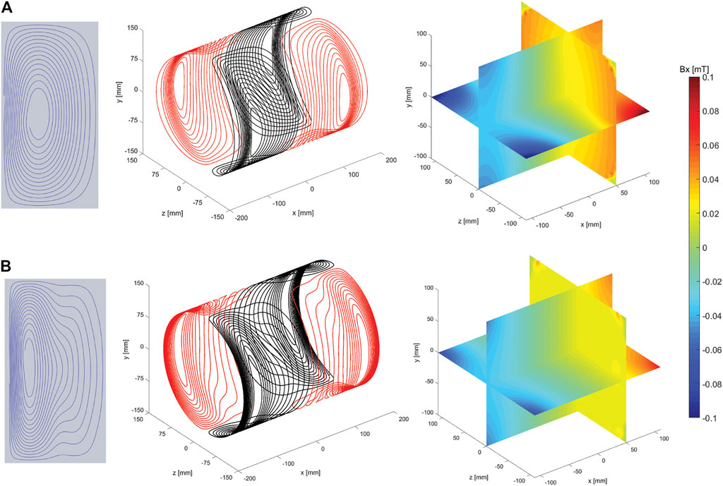
FIGURE 1. From left to right: illustrations of the wire paths of a single quadrant, illustration of the coils and the corresponding simulated magnetic field plots, for the original (A) and new method (B). Simulated magnetic fields created with 1 A driving current. The transverse plane slices are shown at x = 50 mm.

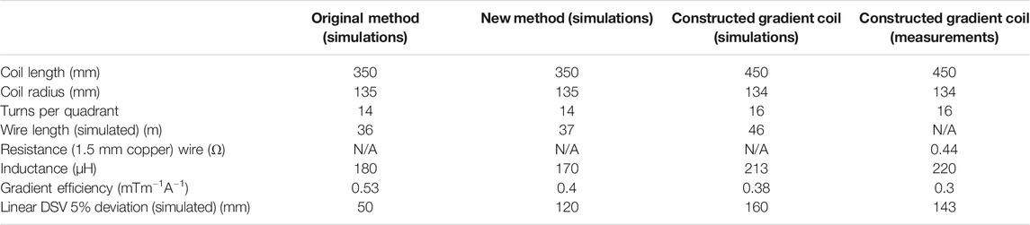
TABLE 1. Characteristics of the simulated gradient coils designed using the original method and the new method (axial length 350 mm) and the actual constructed longer coil (450 mm) designed with the new method.

In order to take further advantage of the intrinsic increased linearity of coils designed using the new method, a 450 mm long gradient coil is designed and built, using the target fields, number of modes and diameter as discussed above. The optimal $\text{λ}$ is found to be 1 e-14. As shown in Table 1 the simulated linear DSV that falls within a 5% error is equal to 160 mm for the constructed coil.

The gradient coil is built using enamelled copper wire with a diameter of 1.5 mm pressed into a 3D printed (Raised 3D pro2 plus) cylindrical holder made from Polylactic acid (PLA) with a wall thickness of 4 mm. The holder has 1.7 × 1.7 mm² square slots in which the wires fit tightly. Loctite super glue-3 is used to keep the wires in place, photographs of the old and new coils can be found in the Supplementary Figures.

A phantom consisting of many “point-sources” is used to verify the simulation results. The phantom is cylindrically shaped, with a length of 20 cm and a diameter of 20 cm. The phantom consists of 16 vertically stacked, laser-cut, PMMA trays. Each tray holds 185 SupraD soft shell, pearl shaped, vitamin D pills. The pills have a diameter of 7 mm and a shell thickness of 0.5 mm. The core consists of sunflower oil in which the vitamins are dissolved. The centre of the pills are separated by 13 mm in all directions. The T₁ and T₂ values of the pills were measured to be 120 and 100 ms, respectively. Photographs of the phantom are shown in the Supplementary Figures.

The solenoid used to image the phantom has a diameter of 25 cm, a length of 25 cm and a Q-factor of 69. Figure 2A shows images of the centre planes of the phantom obtained using a three-dimensional turbo spin echo (TSE) sequence, with sequence parameters outlined in the figure caption. In red the “ground truth” is masked on top of the image. The outer circle denotes the 20 cm DSV. To ensure spatial distortions observed originate predominantly from the gradient non-linearities and not from B₀ in homogeneities, the double phase encoded planes are shown. These are obtained by performing three different TSE scans, each with the frequency encoding in a different direction. The phantom images show signal fading at the edges of the field of view due to the low B₁ at the extremities of the RF coil. The 5% linear DSV is determined by obtaining the displacement of the centre of each signal source with respect to the centre linear line.

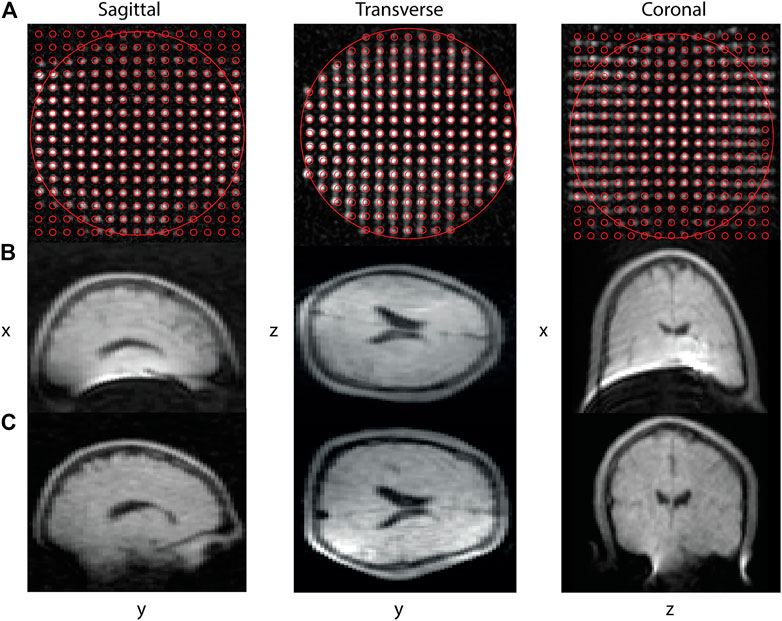
FIGURE 2. Centre planes of a point source phantom imaged using a TSE sequence (A). From left to right: Sagittal, transverse and coronal centre planes are displayed with the following acquisition parameters: 230 (z: right-left) × 230 (x: head-feet) × 230 (y: posterior-anterior) mm³, data matrix: 150 × 150 × 150, TR/TE: 200/15 ms, echo train length: 6, scan duration 12 min 30 s. The small red circles denote the ground truth position of the point sources, the larger circle displays the 200 mm DSV. The lower part of the figure shows in vivo brain images of the same volunteer acquired with the old (B) and new gradient coils (C). The slices are acquired using a TSE sequence with acquisition parameters: 180 (z: right-left) × 240 (x: head-feet) × 220 (y: posterior-anterior) mm³, data matrix: 90 × 120 × 55, TR/TE: 400/15 ms, echo train length: 5, scan duration 9 min 36 s. For the in vivo and phantom images standard Fourier reconstruction with a sine bell squared filter are used.

In vivo brain images of a healthy volunteer were made with the old and the new gradient coil. The dimensions of the old gradient coil are those of the simulated comparison coil listed in the first column of Table 1. A TSE imaging sequence is used for all in vivo measurements: the sequence parameters are presented in the figure captions. For the reconstruction, conventional inverse Fourier transform combined with a sine bell squared k-space filter is used. Figure 2B shows results for the old, and Figure 2C for the new gradient coil.

We note that the transverse gradient coils can also be designed using the new method. However, the resulting wire patterns are essentially the same as when designed with the original method. This is because the target fields corresponding to these coils are constant in the axial direction, and the lower order harmonics proposed in the previous method are sufficient to produce these fields accurately.

Design of a Four-Channel Radio Frequency Coil Array

All of the low-field systems outlined in the introduction use a single transmit and receive coil, using a variation on a solenoid with either variable diameter or variable winding pitch. In contrast, phased array receiver coils [38] are widely used on clinical MRI systems due to their improved signal-to-noise ratio (SNR) compared to larger volume coils, and for their capability of accelerating scans by under sampling k-space [39]. Although the coil-dominated loss at lower field strengths means that the intrinsic increase in SNR is much lower than at higher fields, phased array coils can still be used to reduce the imaging time and enable lossless receive bandwidth amplification via preamplifier impedance mismatch. More importantly, the design of phased arrays receivers on low field systems is more challenging than at conventional fields since coil/sample coupling is much lower, loaded Q-values are higher, and as a result inter-coil coupling is higher. For the same reasons there is strong coupling between the transmit and receive array which requires high-performance detuning circuitry. Conventional PIN-diodes are not effective in the low MHz range and so other actively switching components must be used. One example of a low field array has been presented previously [15], but this used surface loops only, many of which had very low sensitivity since the B₀ and B₁ directions are coincident. The design considered here takes the transverse B₀ direction into account by choosing array elements which are different from the ones used in conventional MRI. We designed a four coil receive array for in vivo imaging of the knee or calf muscle with a diameter of 15 cm using a combination of loop (6 × 10 cm²) and butterfly coils (15.5 × 13.5 cm²) as well as an 18 cm long solenoidal transmit coil with a diameter of 20 cm which has a fast-decoupling field effect transistor (FET)-based switch.

EM simulations are performed using CST Studio Suite 2019 (CST, Darmstadt, Germany). The frequency‐domain solver is used with electric boundary conditions set at 10 cm distance from the coils. The impedance matching network for each coil is implemented by simulating discrete tuning and matching capacitors. A cylindrical phantom (12 cm diameter and 15 cm length) with tissue properties (ε = 61, σ = 0.029 S/m, at 2.15 MHz) matching those of the knee² is placed at the centre of the coils. The Tx coil uses a sigmoidal function of winding pitch for the solenoid. Coupling between the adjacent butterfly and loop coils is minimized by empirically varying the distance between neighbouring elements, and finding that 10.25 mm gaps are optimal for this configuration.

The simulated B₁⁺ field of the solenoid coil is shown in Figures 3A,B: the field is homogeneous to within 1 and 13% over a centre line of 10 cm for the radial and axial directions, respectively. Figure 3C shows the simulated fields of the receive array for each individual element, and the sum of squares. The left part of Table 2 shows the simulated S parameter-matrix (in blue) for each of the Rx coils under loaded conditions. The inter-element coupling for neighbouring coils is very small, with much larger (up to −11 dB) coupling occurring between opposite butterfly elements.

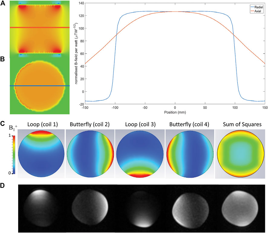
FIGURE 3. Simulated fields of the transmit coil, axial (A) and transverse (B) slices are shown together with values of the magnetic flux density taken along the centre lines. The fields corresponding to the receive array are depicted in the bottom images (C), which shows a CST model of the array loaded by a cylindrical phantom with ε = 61, σ = 0.029 S/m, at 2.15 MHz. The B1 is normalized to 1 W input power. (D) phantom measurements obtained with a cylindrical phantom of the same dimensions as the simulated phantom, the following acquisition parameters were used: 200 (z: right-left) × 200 (y: posterior-anterior) × 300 (x: head-feet) mm³, data matrix: 100 × 100 × 60, TR/TE: 200/15 ms, echo train length: 6, scan duration 3 min 33 s.

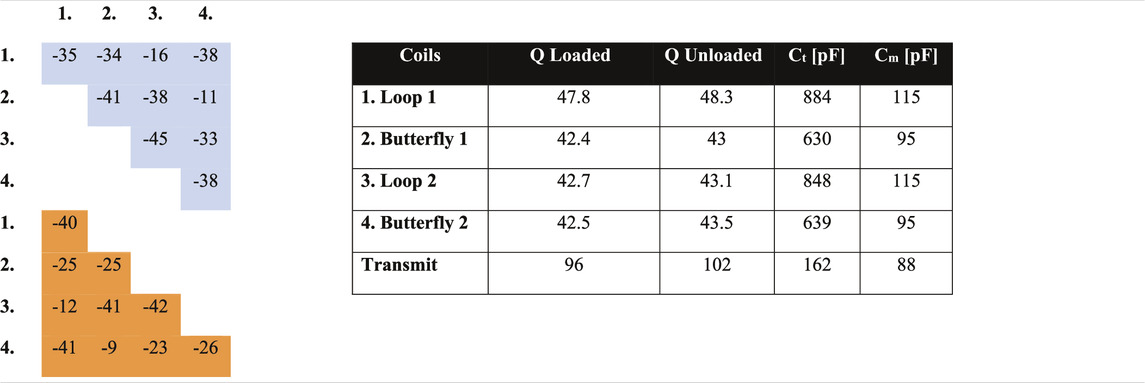
TABLE 2. Left) Simulated (blue) and measured (orange) S-parameter matrix (dB) under loaded conditions. Right) Loaded and unloaded Q values for the Tx coil and Rx coils including tuning and matching capacitor values. Variable capacitors were used in parallel with all Ct and Cm except for transmit coil where the variable capacitor is added to one of the segmentations. The numbers in the left part of the table correspond to the coils in the right part of the table.

Radio Frequency Coil Array Construction

The transmit solenoid coil is constructed using 31 turns of 1 mm copper wire on a 3D-printed cylinder with 20 cm diameter and 18 cm length (Figure 4A). The receive coils are fabricated using 0.8 mm copper wire placed on 3D-printed bases and fixed on a plexiglass cylinder with 15 cm diameter (Figure 4B). The loop and butterfly coils have 5 and 3 turns, respectively. For the Tx coil, capacitive segmentation into three serially-connected sections was performed using capacitors of the same value as the tuning capacitor (C_t). These values together with the Q-values of the coils unloaded and loaded with a saline phantom can be found in the right part of Table 2. For all coils an L-matching network was used.

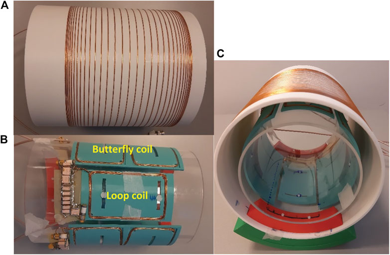
FIGURE 4. Transmit solenoid coil (A), 4-channel array coils (B) and the integrated assembly (C).

Power metal oxide semiconductor field-effect transistors (MOSFETs) are appropriate counterparts for PIN diodes at low frequency [40]. The switching delay was measured to be ∼10 µs at 2.15 MHz. Figure 5 shows the circuit diagram of the MOSFET switch inserted into the impedance matching circuit of the Tx coil. A single 9-V battery is used to power the supply switch, and a voltage regulator (LM317BT, STMicroelectronics, Geneva, Switzerland) to step the voltage up to 12 V to switch the MOSFET (IRLIZ44N, Infineon Technologies AG, Germany). The TTL signal from the spectrometer is fed to an optocoupler (HCPL-2201-000E, Broadcom, United States) to switch the MOSFET gate voltage between 0 and 12 V. To detune the transmit coil an LC resonant “trap” circuit tuned to 2.15 MHz using an inductor and capacitor as well as the parasitic capacitance of the MOSFET. This is added between the drain and source of the MOSFET to detune the coil when the switch is off. An additional LC trap is placed on the ground of the MOSFET to block RF flow to the ground. The RX coils are passively detuned using crossed diodes (BAT6804E6327HTSA1, Infineon Technologies AG, Germany) and additional inductors and capacitors in parallel to the tuning capacitor to form an LC trap at 2.15 MHz. The S-parameters obtained experimentally are shown in orange in the left part of Table 2.

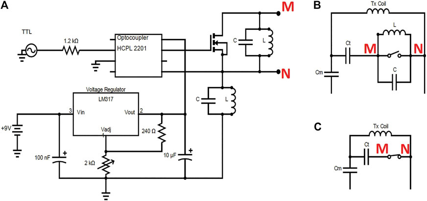
FIGURE 5. The MOSFET switch circuit (A), and Tx coil impedance matching circuit when switch is on (B) and off (C). Note that when the TTL signal is on, the switch is off, and vice-versa.

Phantom images were performed using a TSE sequence on a 12 cm diameter 15 cm length cylindrical phantom, which is the same size as the simulated phantom. The T₁ and T₂ values of the phantom were measured to be 95 and 48 ms respectively. The results of the individual elements, sum of squares reconstruction and the sequence description can be found in Figure 3D. The phantom measurements are in good agreements with the coil profiles found in the simulations.

In vivo TSE knee images are acquired using the array. Figure 6 shows the images obtained with each element, as well as a sum-of-squares reconstruction. Sequence parameters are described in the figure heading. An inverse Fourier transform combined with a sine bell squared filter was used for reconstruction. In agreement with the simulated and measured S-parameters there is very low coupling between adjacent elements because of the low mutual inductance, but signal coupling between opposite butterfly elements is apparent due to the very low loading of the sample.

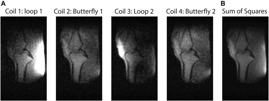
FIGURE 6. Sagittal slice TSE images of the knee. (A) individual elements. (B) sum of squares. parameters: 150 (z: right-left) × 165 (y: posterior-anterior) × 150 (x: head-feet) mm³, data matrix: 200 × 110 × 50, TR/TE: 300/15 ms, echo train length: 4, scan duration 6 min 53 s.

Design of a Battery-Powered Gradient Amplifier

As part of making low-field systems sustainable, the electronics should be as robust as possible with respect to operating conditions, be easily repairable, and ideally be able to run off battery power for operation in remote regions. This section describes an improved version of a three-axis current-output gradient amplifier [17] (designed and built by the Technical University of Delft) which makes it more robust and sustainable. Design specifications for the new amplifier were: maximum current to the load +/−15 Amps, maximum duty cycle 30% per channel, inductance of the gradient coil between 20 and 300 μH, a rise time 50 μs which results in a bandwidth of 7 kHz, overload protection, driving a coil with equivalent series resistance of 0.4 Ω and a parasitic parallel capacitance between the gradient coils estimated at 130 pF. The amplifier is designed to run off an external power source with a supply voltage between +/−10.5 and +/−15 V. To facilitate the use of batteries, where the voltage drops as the battery discharges, the biasing of the amplifier is made relative to the relevant power supply rails. When the batteries are drained an under-voltage lock-out disables the amplifiers at a threshold voltage of 10.5 V. Two 20 Amp car fuses (ATO Blade) are used for protection at the positive and negative terminals.

A schematic of one of the channels of the battery-operated gradient amplifier (each channel is identical) and a photograph of the gradient amplifier can be found in the Supplementary Material. At a 3 A average discharge current, which is typical for an imaging session, the batteries last 5–6 h.

A four-layer PCB configuration was designed with each layer designed for a specific purpose: the upper layer 1 has most of the components for easy access, replacement and routing, layer 2 is a ground layer for thermal stability and optimal heat spreading which is separated per channel to prevent cross coupling, layer three routes the power and layer four contains the high power components with wide copper tracks.

System Characterisation

Having described in detail the improvements in the current setup for the 50 mT low-field imaging system, the final section outlines detailed measurements of the performance of individual components of the system, as well as that of the integrated system.

Gradient Amplifier Performance

At 2.15 MHz the measured output noise is measured to be −123 dBm/Hz, which is roughly 50 dB above thermal noise. Although an RF shield is placed between the gradient coils and the RF coil, this does not provide sufficient attenuation without it becoming so thick that eddy currents become dominant. Therefore, notch filters, see Figures 7A,B, were designed at the gradient amplifier outputs which give over 40 dB extra attenuation. Noise measurements performed at 2.15 MHz using an RF coil placed at the center of the system show no increase in the measured noise by the spectrometer after the gradient amplifiers were switched on (Section Quality Assurance protocol and overall system noise characterisation and measurement over time).

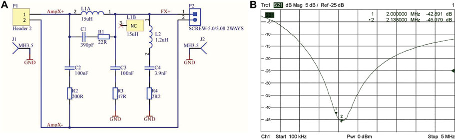
FIGURE 7. Filter design for gradient amplifier output on each channel (A), S₂₁ plot of the output filters on each channel of the gradient amplifier (B).

Figure 8 shows the step response of one of the channels when driving an inductance of 213 µH with an ESR of 0.32 Ω, which corresponds to the values of a typical gradient coil for our application. The waveforms show high fidelity at lower driving currents, whereas it is clearly seen that at 15 A the output starts to limit the slew rate because of clipping to the supply rail.

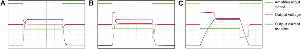
FIGURE 8. Step response of the amplifier as a function of driving current for a gradient coil with resistance 0.32 Ω and inductance 213 μH. The ramp time is 5 µs and the plateau duration 500 µs. The amplifier input signal is shown in green, the output voltage is shown in red, and blue shows the output of the current monitor for a targeted output current of 5 A (A), 10 A (B) and 15 A (C). At 15 A the output starts to significantly limit the slew rate because of clipping to the supply rail.

Radiofrequency Amplifier Performance

Schematics and details of the 1 kW RF amplifier used on the Halbach-based system have been provided as supplementary material to a previous publication [17], but no system performance was reported. Here, testing was performed using a four-channel digital oscilloscope (Teledyne LeCroy HDO 4034A 350 MHz). A sequence of 100 μs pulses were output from the Magritek Kea-2 spectrometer, with an unblanking 5 V TTL pulse applied 20 μs before each RF pulse, and returning to 0 V immediately after each RF pulse. Measurements were performed at: i) the input of the RF amplifier, ii) the output of the RF amplifier, iii) the output of the internal transmit/receive switch, and iv) at the RF coil via a loosely-coupled unmatched pick up loop.

Figure 9 shows digital traces of a 100 µs pulse at different stages of the transmit chain. Figure 9A shows the output of the RF amplifier, where several features of the amplified pulse are labelled with their values listed in Table 3. Figure 9B shows the pulse after the internal transmit/receive switch of the spectrometer. Lastly, Figure 9C shows the signal measured by an un-tuned pick up loop placed inside a tuned solenoidal coil with a Q value of ∼90. The low frequency transients after the transmit/receive switch are filtered out by the tuned RF coil. The long rise-time and fall-time of the RF pulse caused by the high Q of the coil are apparent. There is a delay (400 µs) to allow pulse ringdown after each of the 100 µs pulses before the gradient pulses are applied in the 3D sequences: since the interpulse delays are on the order of 5–10 ms for in vivo imaging experiments this delay is not significant.

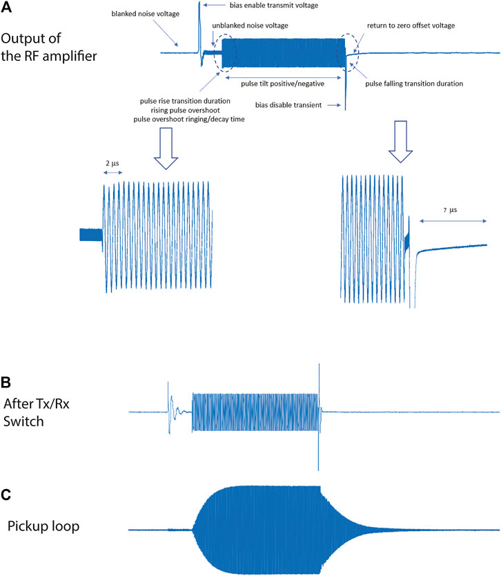
FIGURE 9. Digital traces of a 100 µs pulse at different stages of the transmit chain. The expanded views (A) show different features of the amplified pulse shape. The 2.15 MHz square pulse is 100 μs long, preceded by a 5 V TTL un-blanking trigger signal 20 μs prior to the RF pulse. The same signal is shown after the Tx/Rx switch (B) and received by a un-tuned pickup loop (C).

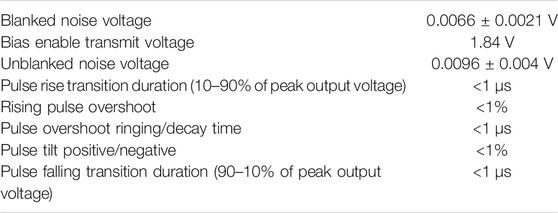
TABLE 3. Measured pulse characteristics at 2.15 MHz at the output of the RF amplifier.

In addition, the voltage gain of the amplifier was measured across a frequency range 1–5 MHz. This was performed using the four-channel digital oscilloscope by comparing the amplitude of the 100 µs pulse before and after it went through the RF amplifier. The results are shown in Figure 10A, which shows a flat response with only ∼2 dB variation across the entire frequency range. The linearity of the response at 2.15 MHz was measured as a function of input power from −50 to −2 dBm: as shown in Figure 10B the gain is within 2.8 dB for values from −50 to −10 dBm, with only substantial variations from uniformity for powers greater than −5 dBm.

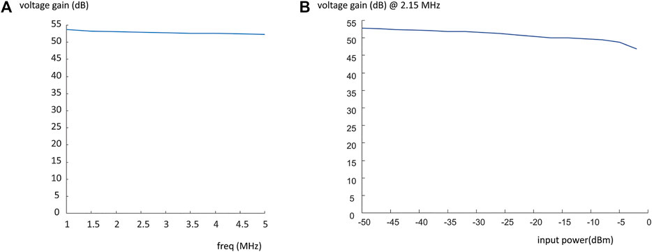
FIGURE 10. Plot of voltage gain vs. frequency (A), and the voltage gain at the operating frequency of 2.15 MHz vs. input power from the Kea spectrometer (B).

Eddy Current Characterisation

In conventional superconducting MRI systems, eddy currents are created primarily by the interaction of the pulsed gradient fields with the metallic bore of the magnet. These interactions are minimized by actively shielding the gradients [33]. The quantification and correction of these effects are well documented in conventional systems [41–45]. In Halbach-based systems eddy currents produced by this interaction might be expected to be much lower, since the magnetic material is discretized into small elements, and the copper RF shield placed between the RF coil and gradient coils is much thinner than the skin depth at low frequencies.

The effects of the eddy currents were measured using a standard spectroscopic method. A 4 mT/m, 20 ms square gradient pulse is applied. The length of the gradient pulse is chosen so that the eddy current measurements were dominated by the falling edge of the gradient pulse rather than a combined effect of the rising edge and falling edge, which is the case if a shorter gradient pulse is applied. The value of 4 mT/m is ∼90% of the maximum gradient strength obtainable with the system described here. The pulse is followed by a variable delay time, before an RF pulse is applied to produce a free induction decay. The peak intensity of the spectrum is recorded as a function of this delay. Three readings were made for each value to estimate the standard deviation of each measurement. Measurements were performed for the three gradient coils separately. Figure 11 shows the measured peak amplitudes for each gradient coil. The eddy current effects are approximately the same for the y- and z-gradient which have the same geometry but are rotated by 90^o with respect to one another. The x-gradient, has a different shape and shows longer time-constant eddy currents, possibly due to it being the closest to the shield.

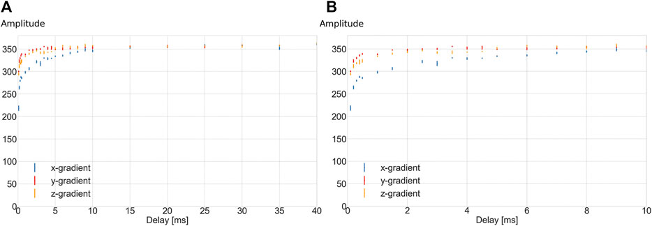
FIGURE 11. Signal amplitudes (arbitrary units) of the magnitude spectrum as a function of the delay time after the gradient has been turned off, before the spectrum is acquired. Full extent of delay times up to 40 ms (A), and zoomed view of the first 10 ms of the data (B). The average and standard deviation of four measurements per delay time are displayed. Blue: x-gradient, red: y-gradient, yellow: z-gradient.

Quality Assurance Protocol and Overall System Noise Characterisation and Measurement Over Time

Since portable systems are intended to operate in conditions outside those characterised by tightly controlled temperature and humidity, as well as an RF shielded environment, it is important to have a rapid assessment of the performance of each of the individual components of the system. In addition, it is very useful to check over a longer period of time whether system performance degrades, and which component(s) is/are responsible for this. To this end a simple 30-min quality control protocol is set up which consists of:

i) Checking the impedance matching of the coil at 2.15 MHz: the S₁₁ should be less than -20 dB or the coil should be retuned.

ii) Determination of the resonance frequency with all shims set to zero. The resonance frequency is highly dependent upon the time after a previous in vivo scan has been acquired, since the magnets heat up in such experiments due to passive thermal emission from the body, and so the resonance frequency decreases (our estimate for the maximum shift is about 1 kHz immediately after a 45 min scan, and one measurement immediately after an in vivo scan was included to demonstrate this effect). For this reason, the quality control measurement is performed a significant time after in vivo measurements, as it is intended to monitor the very long-term stability of the magnet, since it is known that NdBFe slowly demagnetizes over time.

iii) Averaging five noise measurements with only the spectrometer turned on and the output/input of the Tx/Rx switch connected to the coil. This determines whether the coil picks up noise signals which means that any shielding or noise reduction in place is not functioning sufficiently. The Magritek console outputs a reference 1 μV signal, and measures the noise voltage with respect to this internal standard. The precision of the reference voltage is 0.01 μV. The noise is measured with the maximum receiver gain and so any quantization noise is much less than the noise level.

iv) Averaging five noise measurements with the spectrometer and the RF amplifier turned on and the output/input of the Tx/Rx switch connected to the coil. This determines whether the RF amplifier contributes to the noise.

v) Averaging five noise measurements with the spectrometer, the RF amplifier and the gradient amplifier turned on and the output/input of the Tx/Rx switch connected to the coil. This determines whether the gradient amplifier contributes noise, i.e., there may be a problem with the gradient filters.

vi) Calibration of the power required for a 90^o pulse to ensure that coil components have not degraded over time. For the 90° pulse the variation from day-to-day is less than 0.3 dB, so anything consistently outside this range indicates that the coil Q has degraded.

vii) Measuring the SNR in 2D projection spin echo images using three different combinations of the gradient coils: frequency encoding gradient x and phase encoding gradient y, frequency encoding gradient z and phase encoding gradient x, and frequency encoding gradient y and phase encoding gradient z. The spectrometer has a specific protocol for measuring the noise level with respect to an internal 1 μV standard signal. For the SNR measurements regions-of-interest were defined within the object (signal) and outside the object (noise). The measurements have a variation of ∼7% which indicated that anything outside of this range should be checked further.

viii) Obtaining a simple spectrum after application of a 90° pulse in order to measure the lineshape. This measurement is made after first order shimming via the linear gradients. To estimate the effect of a malfunctioning gradient coil we performed one set of measurements with each of the coils disconnected in turn.

A 3D phantom holder is designed to make positioning inside the RF coil and magnet highly reproducible. The phantom is a sphere of 74 mm diameter containing a copper sulphate doped (3 mM) agar mixture (0.5%) and has a T₁ value of 227 ms and T₂ of 224 ms. It is placed inside a transmit/receive solenoidal coil (inner diameter of 147 mm, outer diameter of 155 mm, length 170 mm, 1 mm copper wire, Q value 89), which can be positioned accurately via markings inside the scanner. Photographs of the solenoid, phantom and holder are shown in the Supplementary Figures. The protocol discussed above has been run over the course of several weeks and the results are discussed below.

Figure 12A shows the frequency is stable over a longer period of time with the measurements taken once a day on average, over a course of six weeks, a significant time after in vivo experiments have been performed. A decrease in frequency can be observed in the last week, the likely cause is that this week was particularly warm. The increase in the temperature is likely to be the cause of this field drift. One outlier can be observed which was obtained after an entire day of in vivo scanning: the field drift was caused by an increase of temperature caused by the human body, as expected. This type of field drift can be corrected for when performing in vivo experiments as described by [18]. Figure 12B shows the RMS noise measured over a bandwidth of 50 kHz, with no RF pulses applied, the data are obtained over the course of 6 weeks. No significant differences are observed when switching on the RF and gradient amplifiers. The noise measurement appears to have a variation of less than 10% (which is also limited by the resolution of the measurement on the system), and so anything beyond 20% is indicative of either very broadband interference or some problem with the preamplifier or receiving chain. Figure 12C shows the SNR measured from imaging data over the period of 4 weeks. The left side of Figure 12D shows four spectra acquired on three different days: the right side of the figure shows the effects when one of the gradients were disconnected showing a very obvious deterioration in performance.

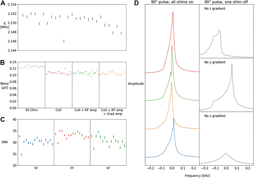
FIGURE 12. The f₀ frequency measurements measured in the course of 6 weeks with an average of one scan per day (A). Noise measured using five averages obtained in the course of 6 weeks with the coil connected, and the coil connected with respectively only the RF amplifier on and both the RF and gradient amplifiers turned on (B). SNR measurements obtained over a period of 2 weeks for the three encoding directions (C) (frequency/phase encoding). The magnitude spectrum on different occasions measured over the course of a 3 days, with all shims on (left), and the effects on the magnitude spectrum when one of the shims is not functioning correctly (D).

Discussion

In this paper on-going developments of a 50 mT Halbach-based portable MRI system for in vivo imaging have been discussed. In addition to specific hardware improvements including a gradient coil with increased region of linearity, a four-element phased array receive coil, and a battery-operated gradient amplifier, detailed system characterisations of eddy currents, RF transmitter performance, and quality control protocol have been shown.

The comparison of two axial gradient coils simulated for the same target DSV, but designed using two different target field methods, demonstrated that for fixed dimensions, in simulations, the new method increases the 5% linear DSV by ∼150%, traded against a decrease in efficiency of ∼25%. The improvement in linearity is confirmed with phantom measurements. This home-made inexpensive point source phantom proved to be a powerful tool for displaying the current capabilities and limits of the system. In the future the phantom can be used to calibrate new low field systems. The linearity measured differed slightly from the simulations, one reason for this is that the pills introduce a relatively large discretisation error with respect to the smoother simulated data. The increase in axial linearity allows the whole adult brain to be imaged with little geometric distortion, at a spatial resolution of ∼2 mm using the maximum output of 4 Amps from the gradient amplifier. The reduced gradient efficiency comes about primarily due to the large number of very closely spaced turns at the ends of the gradient coils, which are used to increase the linearity. The trade-off between linearity and efficiency will be further investigated, particularly given that for spatial resolutions on the millimetre scale the distortions created by small non-linearities can be relatively easily corrected via post-processing [46]. Another area which will be investigated is the design of asymmetric axial gradient coils [47, 48]. Due to the relatively small magnet bore positioning of the subject’s head at the centre of the magnet/gradient is restricted by the shoulders. This means that for all of the images currently acquired, the centre of the brain lies towards the front of the magnet, and if the subject has a relatively short neck the lower part of the brain may coincide with an area of poor B₀ homogeneity and close to the region where the axial gradient coil linearity begins to deteriorate. Cooley et al. have used boundary element methods to design an asymmetric axial gradient coil with variable diameter and the zero gradient point towards the bore entrance [13]. Such a design is also possible using asymmetrical target fields and the approach outlined in this paper.

Although not common at the moment, receive arrays could be used to reduce the time required for image acquisition, if the SNR is sufficient, by utilizing parallel imaging reconstruction of under-sampled data. In this paper we showed a basic four-element array comprised of two surface coils and two butterfly-shaped coils. The coils were reasonably decoupled from each other geometrically, but the decoupling could be increased by the use of low input impedance preamplifiers. Since coil loss is dominant at low frequency, and inter-coil coupling therefore much higher, the input impedance of such preamplifiers must be much lower than for commercial systems, so <<1 Ohm, which would require a custom design. Multiple low loss transmit/receive switches would also be required to be designed and constructed for these low frequency systems.

Designing the gradient amplifier to be battery powered demonstrated the first steps in making the system independent of the power grid, and thus well suited for low resource and remote settings. The maximum current output of ∼15 Amps is much lower than that of ones used in commercial scanners, and may need to be increased if applications in musculoskeletal MRI, for example, are to be targeted, in which case sub-millimetre resolution is required. Currently we do not use any pre-emphasis in the system to compensate for eddy currents, this would require the capability to provide a large over-voltage, which might compromise the desire to have only air-cooling of the amplifier.

Finally, we presented some very simple quality checks of the noise and SNR levels when different components of the system are turned on. Since all designs are available open-source, this information allows interested researchers to construct systems based on all or a subset of the hardware described. Additionally, the system characterisation gives a baseline for future studies to compare the performance obtained with different custom-built or commercial low-field systems.

Data Availability Statement

The raw data supporting the conclusion of this article will be made available by the authors, without undue reservation.

Ethics Statement

Ethical review and approval was not required for the study on human participants in accordance with the local legislation and institutional requirements. Written informed consent from the participants OR participants legal guardian/next of kin was not required to participate in this study in accordance with the national legislation and the institutional requirements.

Author Contributions

BV designed and built the gradient coils, performed measurements. Collected and reformatted the data and figures from other project members, wrote a part of the manuscript and did the formatting. JP designed and built the RF (radio frequency) coil array, wrote the draft text for this part and supplied the corresponding figures. ZA designed and built the transmit receive (TR)-switches and pre-amplifiers used during image acquisition. WT contributed to the practical design of the gradient coils and magnet, and assisted with the installation of the new gradient coil. DG designed and built the gradient amplifiers and supplied the documentation. CV designed and performed the quality control protocol, delivered the corresponding figures and text. RR helped with the mathematical framework and the design of the newly proposed gradient design method and proofread part of the manuscript. TO’R created the magnet system, contributed to the design of the RF-array, specified the design parameters for the new gradient amplifier and acquired the in vivo images. AW performed measurements, wrote part of the manuscript, proofread manuscript, produced figures.

Funding

Partial funding for this project was provided by Horizon 2020 European Research Grant FET-OPEN 737180 Histo MRI (TO’R), Horizon 2020 ERC Advanced NOMA-MRI 670629 (AW), and a Simon Stevin Meester Prize (BV, AW), H2020-MSCA-ITN-ETN 859908 (JP) and NWO WOTRO award (DG).

Conflict of Interest

JP was employed by Percuros BV

The remaining authors declare that the research was conducted in the absence of any commercial or financial relationships that could be construed as a potential conflict of interest..

Publisher’s Note

All claims expressed in this article are solely those of the authors and do not necessarily represent those of their affiliated organizations, or those of the publisher, the editors and the reviewers. Any product that may be evaluated in this article, or claim that may be made by its manufacturer, is not guaranteed or endorsed by the publisher.

Supplementary Material

The Supplementary Material for this article can be found online at: https://www.frontiersin.org/articles/10.3389/fphy.2021.701157/full#supplementary-material

Supplement Figure 1 | Photographs of the constructed gradient coils where 1.5 mm diameter enameled copper wire is pressed into the grooves of a 3D printed cylindrical mold, shown for the old (A) and new method (B).

Supplement Figure 2 | Photograph of point source phantom together with a single layer.

Supplement Figure 3 | A schematic of one of the channels of the battery-operated gradient amplifier.

Supplement Figure 4 | Photograph of the Gradient amplifier.

Supplement Figure 5 | Photograph of the quality assurance phantom, inside the solenoidal coil.

Footnotes

¹Gradient design Tool: https://github.com/LUMC-LowFieldMRI/GradientDesignTool

²IT’IS database for thermal and electromagnetic parameters of biological tissues: https://itis.swiss/virtual-population/tissue-properties/overview/

References

1. Tsai LL, Mair RW, Rosen MS, Patz S, Walsworth RL. An Open-Access, Very-Low-Field MRI System for Posture-dependent 3He Human Lung Imaging. J Magn Reson (2008) 193:274–85. doi:10.1016/j.jmr.2008.05.016
2. Tsai LL, Mair RW, Li C-H, Rosen MS, Patz S, Walsworth RL. Posture-dependent Human 3He Lung Imaging in an Open-Access MRI System. Acad Radiol (2008) 15:728–39. doi:10.1016/j.acra.2007.10.010
3. Sarracanie M, LaPierre CD, Salameh N, Waddington DEJ, Witzel T, Rosen MS. Low-cost High-Performance MRI. Sci Rep (2015) 5:5. doi:10.1038/srep15177
4. Choi C-H, Hutchison JMS, Lurie DJ. Design and Construction of an Actively Frequency-Switchable RF Coil for Field-dependent Magnetisation Transfer Contrast MRI with Fast Field-Cycling. J Magn Reson (2010) 207:134–9. doi:10.1016/j.jmr.2010.08.018
5. Ross PJ, Broche LM, Lurie DJ. Rapid Field-Cycling MRI Using Fast Spin-echo. Magn Reson Med (2014) 73:1120–4. doi:10.1002/mrm.25233
6. Macleod MJ, Broche L, Ross J, Guzman-Guttierez G, Lurie D. A Novel Imaging Modality (Fast Field-Cycling MRI) Identifies Ischaemic Stroke at Ultra-low Magnetic Field Strength. Int J Stroke (2018) 13:62–3. doi:10.1177/1747493018801108
7. Bödenler M, de Rochefort L, Ross PJ, Chanet N, Guillot G, Davies GR, et al. Comparison of Fast Field-Cycling Magnetic Resonance Imaging Methods and Future Perspectives. Mol Phys (2018) 117:832–48. doi:10.1080/00268976.2018.1557349
8. Broche LM, Ross PJ, Davies GR, MacLeod M-J, Lurie DJ. A Whole-Body Fast Field-Cycling Scanner for Clinical Molecular Imaging Studies. Sci Rep (2019) 9:9. doi:10.1038/s41598-019-46648-0
9. He Y, He W, Tan L, Chen F, Meng F, Feng H, et al. Use of 2.1 MHz MRI Scanner for Brain Imaging and its Preliminary Results in Stroke. J Magn Reson (2020) 319:106829. doi:10.1016/j.jmr.2020.106829
10. Nakagomi M, Kajiwara M, Matsuzaki J, Tanabe K, Hoshiai S, Okamoto Y, et al. Development of a Small Car-Mounted Magnetic Resonance Imaging System for Human Elbows Using a 0.2 T Permanent Magnet. J Magn Reson (2019) 304:1–6. doi:10.1016/j.jmr.2019.04.017
11. Sheth KN, Mazurek MH, Yuen MM, Cahn BA, Shah JT, Ward A, et al. Assessment of Brain Injury Using Portable, Low-Field Magnetic Resonance Imaging at the Bedside of Critically Ill Patients. JAMA Neurol (2021) 78:41. doi:10.1001/jamaneurol.2020.3263
12. Turpin J, Unadkat P, Thomas J, Kleiner N, Khazanehdari S, Wanchoo S, et al. Portable Magnetic Resonance Imaging for ICU Patients. Crit Care Explorations (2020) 2:e0306. doi:10.1097/cce.0000000000000306
13. Cooley CZ, McDaniel PC, Stockmann JP, Srinivas SA, Cauley SF, Śliwiak M, et al. A Portable Scanner for Magnetic Resonance Imaging of the Brain. Nat Biomed Eng (2020) 5:229–39. doi:10.1038/s41551-020-00641-5
14. McDaniel PC. Computational Design and Fabrication of Portable MRI Systems. Massachusetts: Dissertation Massachusetts Institute of Technology (2020).
15. Cooley CZ, Stockmann JP, Armstrong BD, Sarracanie M, Lev MH, Rosen MS, et al. Two-dimensional Imaging in a Lightweight Portable MRI Scanner without Gradient Coils. Magn Reson Med (2014) 73:872–83. doi:10.1002/mrm.25147
16. Cooley CZ, Haskell MW, Cauley SF, Sappo C, Lapierre CD, Ha CG, et al. Design of Sparse Halbach Magnet Arrays for Portable MRI Using a Genetic Algorithm. IEEE Trans Magn (2018) 54:1–12. doi:10.1109/tmag.2017.2751001
17. O'Reilly T, Teeuwisse WM, Webb AG. Three-dimensional MRI in a Homogenous 27 cm Diameter Bore Halbach Array Magnet. J Magn Reson (2019) 307:106578. doi:10.1016/j.jmr.2019.106578
18. O’Reilly T, Teeuwisse WM, Gans D, Koolstra K, Webb AG. In Vivo 3D Brain and Extremity MRI at 50 mT Using a Permanent Magnet Halbach Array. Magn Reson Med (2020) 85:495–505. doi:10.1002/mrm.28396
19. Obungoloch J, Harper JR, Consevage S, Savukov IM, Neuberger T, Tadigadapa S, et al. Design of a Sustainable Prepolarizing Magnetic Resonance Imaging System for Infant Hydrocephalus. Magn Reson Mater Phy (2018) 31:665–76. doi:10.1007/s10334-018-0683-y
20. Ren ZH, Obruchkov S, Lu DW, Dykstra R, Huang SY. A Low-Field Portable Magnetic Resonance Imaging System for Head Imaging. In: Progress in Electromagnetics Research Symposium - Fall; 2017 Nov 19–22; Singapore. PIERS - FALL (2017). doi:10.1109/piers-fall.2017.8293655
21. Sarracanie M, Salameh N. Low-Field MRI: How Low Can We Go? A Fresh View on an Old Debate. Front Phys (2020) 8:127. doi:10.3389/fphy.2020.00172
22. Raich H, Blümler P. Design and Construction of a Dipolar Halbach Array with a Homogeneous Field from Identical Bar Magnets: NMR Mandhalas. Concepts Magn Reson (2004) 23B:16–25. doi:10.1002/cmr.b.20018
23. Bauer C, Raich H, Jeschke G, Blümler P. Design of a Permanent Magnet with a Mechanical Sweep Suitable for Variable-Temperature Continuous-Wave and Pulsed EPR Spectroscopy. J Magn Reson (2009) 198:222–7. doi:10.1016/j.jmr.2009.02.010
24. Soltner H, Blümler P. Dipolar Halbach Magnet Stacks Made from Identically Shaped Permanent Magnets for Magnetic Resonance. Concepts Magn Reson (2010) 36A:211–22. doi:10.1002/cmr.a.20165
25. Windt CW, Soltner H, Dusschoten Dv., Blümler P. A Portable Halbach Magnet that Can Be Opened and Closed without Force: The NMR-CUFF. J Magn Reson (2011) 208:27–33. doi:10.1016/j.jmr.2010.09.020
26. Blümler P, Casanova F. Chapter 5. Hardware Developments: Halbach Magnet Arrays. In: Mobile NMR and MRI: Developments and Applications. London, United Kingdom: The Royal Society of Chemistry (2015). 133–57. doi:10.1039/9781782628095-00133
27. BlüMler P. Proposal for a Permanent Magnet System with a Constant Gradient Mechanically Adjustable in Direction and Strength. Concepts Magn Reson (2016) 46:41–8. doi:10.1002/cmr.b.21320
28. de Vos B, Fuchs P, O'Reilly T, Webb A, Remis R. Gradient Coil Design and Realization for a Halbach-Based MRI System. IEEE Trans Magn (2020) 56:1–8. doi:10.1109/tmag.2019.2958561
29. Turner R. A Target Field Approach to Optimal Coil Design. J Phys D: Appl Phys (1986) 19:L147–L151. doi:10.1088/0022-3727/19/8/001
30. Zhang B, Gazdzinski C, Chronik BA, Xu H, Conolly SM, Rutt BK. Simple Design Guidelines for Short MRI Systems. Concepts Magn Reson (2005) 25B:53–9. doi:10.1002/cmr.b.20033
31. Turner R. Minimum Inductance Coils. J Phys E Sci Instrum (1988) 21:948–52. doi:10.1088/0022-3735/21/10/008
32. Chronik EA, Rutt BK. Constrained Length Minimum Inductance Gradient Coil Design. Magn Reson Med (1998) 39:270–8. doi:10.1002/mrm.1910390214
33. Carlson JW, Derby KA, Hawryszko KC, Weideman M. Design and Evaluation of Shielded Gradient Coils. Magn Reson Med (1992) 26:191–206. doi:10.1002/mrm.1910260202
34. Forbes LK, Crozier S. Asymmetric Zonal Shim Coils for Magnetic Resonance Applications. Med Phys (2001) 28:1644–51. doi:10.1118/1.1388538
35. Forbes LK, Crozier S. A Novel Target-Field Method for Finite-Length Magnetic Resonance Shim Coils: I. Zonal Shims. J Phys D: Appl Phys (2001) 34:3447–55. doi:10.1088/0022-3727/34/24/305
36. Forbes LK, Crozier S. A Novel Target-Field Method for Finite-Length Magnetic Resonance Shim Coils: II. Tesseral Shims. J Phys D: Appl Phys (2002) 35:839–49. doi:10.1088/0022-3727/35/9/303
37. Brideson MA, Forbes LK, Crozier S. Determining Complicated Winding Patterns for Shim Coils Using Stream Functions and the Target-Field Method. Concepts Magn Reson (2001) 14:9–18. doi:10.1002/cmr.10000
38. Roemer PB, Edelstein WA, Hayes CE, Souza SP, Mueller OM. The NMR Phased Array. Magn Reson Med (1990) 16:192–225. doi:10.1002/mrm.1910160203
39. Hamilton J, Franson D, Seiberlich N. Recent Advances in Parallel Imaging for MRI. Prog Nucl Magn Reson Spectrosc (2017) 101:71–95. doi:10.1016/j.pnmrs.2017.04.002
40. Nacher P-J, Kumaragamage S, Tastevin G, Bidinosti CP. A Fast MOSFET RF Switch for Low-Field NMR and MRI. J Magn Reson (2020) 310:106638. doi:10.1016/j.jmr.2019.106638
41. Kim YS, Cho ZH. Eddy-current-compensated Field-Inhomogeneity Mapping in NMR Imaging. J Magn Reson (1969) (1988) 78:459–71. doi:10.1016/0022-2364(88)90132-1
42. Boesch C, Gruetter R, Martin E. Temporal and Spatial Analysis of fields Generated by Eddy Currents in Superconducting Magnets: Optimization of Corrections and Quantitative Characterization of Magnet/gradient Systems. Magn Reson Med (1991) 20:268–84. doi:10.1002/mrm.1910200209
43. Papadakis NG, Martin KM, Pickard JD, Hall LD, Carpenter TA, Huang CL-H. Gradient Preemphasis Calibration in Diffusion-Weighted echo-planar Imaging. Magn Reson Med (2000) 44:616–24. doi:10.1002/1522-2594(200010)44:4<616::aid-mrm16>3.0.co;2-t
44. Spees WM, Buhl N, Sun P, Ackerman JJH, Neil JJ, Garbow JR. Quantification and Compensation of Eddy-Current-Induced Magnetic-Field Gradients. J Magn Reson (2011) 212:116–23. doi:10.1016/j.jmr.2011.06.016
45. Niederländer B, Blümler P. Simple Eddy Current Compensation by Additional Gradient Pulses. Concepts Magn Reson A (2018) 47A:e21469. doi:10.1002/cmr.a.21469
46. Koolstra K, O’Reilly T, Börnert P, Webb A. Image Distortion Correction for MRI in Low Field Permanent Magnet Systems with strong B0 Inhomogeneity and Gradient Field Nonlinearities. Magn Reson Mater Phy (2021). doi:10.1007/s10334-021-00907-2
47. Tomasi D, Xavier RF, Foerster B, Panepucci H, Tannús A, Vidoto EL. Asymmetrical Gradient Coil for Head Imaging. Magn Reson Med (2002) 48:707–14. doi:10.1002/mrm.10263
Keywords: low field MRI, MR hardware, halbach magnet, gradient coil design, RF coil array, RF amplifier, quality control, gradient amplifier
Citation: de Vos B, Parsa J, Abdulrazaq Z, Teeuwisse WM, Van Speybroeck CDE, de Gans DH, Remis RF, O’Reilly T and Webb AG (2021) Design, Characterisation and Performance of an Improved Portable and Sustainable Low-Field MRI System. Front. Phys. 9:701157. doi: 10.3389/fphy.2021.701157
Received: 27 April 2021; Accepted: 09 July 2021;
Published: 26 July 2021.
Edited by:
Sigrun Roat, Medical University of Vienna, AustriaReviewed by:
Robert Todd Constable, Yale University, United StatesNajat Salameh, University of Basel, Switzerland
Copyright © 2021 de Vos, Parsa, Abdulrazaq, Teeuwisse, Van Speybroeck, de Gans, Remis, O’Reilly and Webb. This is an open-access article distributed under the terms of the Creative Commons Attribution License (CC BY). The use, distribution or reproduction in other forums is permitted, provided the original author(s) and the copyright owner(s) are credited and that the original publication in this journal is cited, in accordance with accepted academic practice. No use, distribution or reproduction is permitted which does not comply with these terms.
*Correspondence: Andrew G. Webb, a.webb@lumc.nl