B₀-Shimming Methodology for Affordable and Compact Low-Field Magnetic Resonance Imaging Magnets

Introduction

In the last decades, magnetic resonance imaging (MRI) developed to one of the most useful medical imaging techniques allowing to depict the structure and function of tissue and organs in a quality, which is unmatched by other clinical imaging modalities. Despite this technological and clinical progress, machines and operation of these machines is still very expensive and restricted to a small portion of the global population of patients [1]. Current MRI magnets mostly rely on cryogenically cooled superconductors to reach high magnetic fields of typically B₀ = 1.5–3.0 T. These high fields drive the complexity and are mainly responsible for the high costs of an MRI [2]. Recently, several efforts emerged investigating the benefits of low field MRI (B₀ < 0.2 T) to provide a low cost, point-of-care alternative [2–7]. The MR magnet design benefits from reduced complexity and costs at lower fields. While in the past most low field MR magnets were based on permanently magnetized iron with a ferromagnetic yoke, more recently permanent magnet designs are based on a Halbach or Halbach type layout, where multiple small magnets are arranged in a specific way [8–12]. These designs have the advantage that less magnetic mass is utilized, making the magnets smaller, more mobile, and less costly. A challenge with these designs is, however, to achieve a good B₀ field homogeneity, which for commercial high field systems is typically below <10 ppm. One way to relax these requirements is to build in fixed gradients into the magnet design which are used for spatial encoding [7, 10–13]. Even for classical imaging applications using switched gradient coils along three dimensions, Halbach based low-field magnet designs were recently able to produce in-vivo imaging of the extremities, the brain [14] and implants [15], which benefits from lower specific absorption rate (SAR) and lower susceptibility artefacts compared to higher field systems. These encouraging results were acquired with a Halbach based permanent magnet that has an inhomogeneity of 2,400 ppm in the target field of view, demonstrating that the requirements on B₀ field homogeneity at low fields are less strict. Spin echo based imaging can be used to generate most contrasts and T₂^* based contrasts utilizing gradient echo imaging techniques that require higher field homogeneities, are much lower at lower fields. Nevertheless, the B₀ homogeneity over the target volume needs to be within the bandwidth of the RF excitation and a strong B₀ inhomogeneity might lead to image distortions.

Even though MR magnets can be designed very homogeneously in numerical simulations [9], translating these results into the practice is very challenging especially in a low-cost setting. The strengths of the magnetic field from neodymium-iron-boron (NdFeB) magnets may vary up to 5% due to material imperfections and the angular variation of the magnetization vector up to 0.9° [16]. The remanence of the magnetic material is sensitive to temperature changes and the positioning and orientation of the many magnets will deviate slightly from the simulated setting e.g., due to forces that are present between the magnets [17].

B₀ shimming work for low-field permanent magnets is so far mostly limited to simulation studies [18], two pole or C-shaped magnets [18, 19] and/or for small shimming volumes focusing on the application of nuclear magnetic resonance (NMR) spectroscopy [20]. Recently low-field MR magnets are being constructed based on genetic algorithms using a dipole approximation to determine the position, orientation and material of the discrete magnets to reach a target field profile [9, 11, 12].

In this work an iterative approach in the design of a low-field MR magnet using Halbach arrays is investigated with the goal to improve B₀ homogeneity. The methodology is tested on a small bore (inner bore diameter = 130 mm) MR magnet with a B₀ field strength of 0.1 T and a target field of view of ∼4 cm in diameter. The strategy is two-fold relying on a compact base magnet design, which consequently is shimmed using a genetic algorithm and shim inserts. The MR magnet can be reproduced with off-the-shelf components and a 3D printer and used e.g., for educational purposes in existing setups [21]. The evaluated shimming techniques improve B₀ homogeneity up to a factor of 8 in the first iteration and the applied methodology is scalable to bigger magnet designs. Design files and code from this work will be made available as open source hardware on opensourceimaging.org.

Materials and Methods

The presented strategy to construct a homogeneous MR magnet consist of two parts:

1) The construction of a base magnetic field with the envisioned B₀ field strengths and inner bore diameter (Figure 1).

2) Shimming of the base magnet using a genetic algorithm to calculate the sizes, locations, and orientations of the shimming magnets, which are inserted in the base magnet design (Figure 2). A requirement of this shimming approach is that the inner or outer dimensions of the base magnet are not modified.

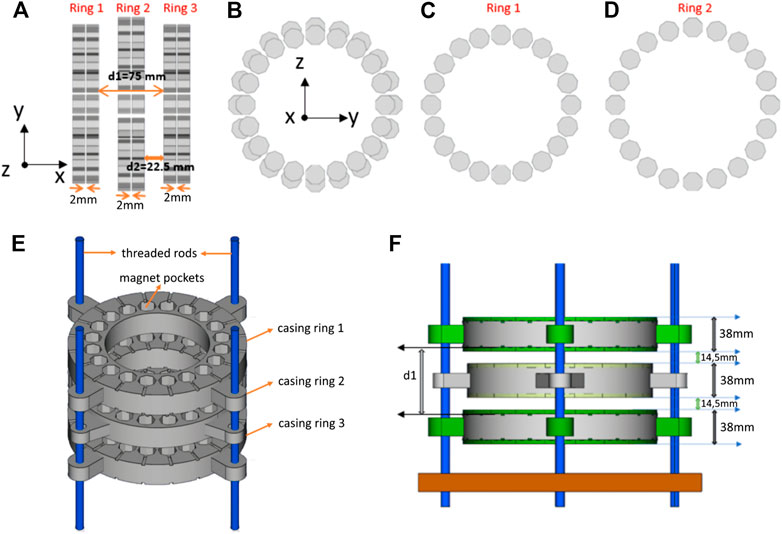
FIGURE 1. Illustration of the base magnet before shimming. (A) Side and (B) Front view on the base magnet depicting the octagonal magnets of Ring 1–3. Front view on (C) Ring 1 (radius r₁ = 80.5 mm) and (D) Ring 2 (radius r₂ = 89.2 mm). (E) 3D renderings of the magnet casing showing the magnet pockets and threaded rods allowing to adjust the correct distance between the rings. (F) Side view of the 3D model of the base magnet including a base plate to mount the threaded rods and lids for each magnet pocket.

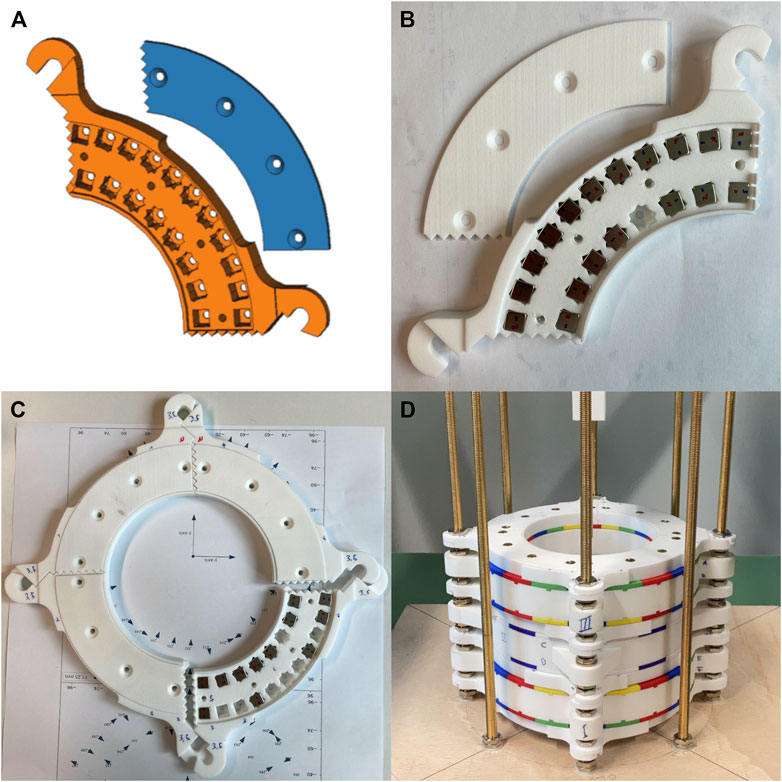
FIGURE 2. Photographs and 3D renderings of the constructed and assembled shim pieces including the 9 mm cubic shim magnets. (A) CAD drawing of a single shim piece (orange) and cover (blue). Please note that the pockets are designed in a way that the shim magnets can be inserted in both radial (k = 1) and Halbach (k = 2) orientation. (B) 3D printed shim piece with inserted magnets and the cover removed. The poles of the magnets are marked with north (N) and south (S). (C) Illustration of a fully assembled shim ring constructed from four shim pieces. (D) Photograph of the fully assembled base magnet including all shim inserts.

The proof of concept of this methodology is tested on a desktop MR magnet with a targeted inner bore diameter of 10 cm (including gradient coils). The size was chosen such that all components can be 3D printed with a standard sized 3D printer.

Simulation Environment and Mathematical Methods

For the base magnet, magnetostatic field simulations were conducted using COMSOL Multiphysics 5.4 (COMSOL AB, Stockholm, Sweden) utilizing the finite element method (FEM). The geometry of the magnets is assumed to be not chamfered. Inside the magnets, the remanent field is set to the appropriate strength, while outside it is assumed μ_r = ε_r = 1.

For the B₀ shimming algorithm, the dipole approximation was used to calculate the magnetic field distribution of each shim magnet [22]:

with the permeability of vacuum ${\mu }_0$ and the location $r$ of the magnetic field with respect to the origin of the magnetic dipole moment (or shim magnet) $m$. For a shim magnet, the magnitude of the magnetic dipole moment $m$ can be calculated by [23].

with the remanence $B_r$ and the magnet volume $V$. Only the z-component is considered, as the magnetic field to be shimmed is oriented along this axis.

Using the weighted orthogonal basis set of real (orthonormalized) spherical harmonic functions Y_lm in spherical coordinates, the z-component of the magnetic field B_z on a sphere with radius r, polar $\theta$ and azimutal $\varphi$ angles is described as

The spherical harmonic coefficients $c_{lm}$, dependent on the degree $l$ and order $m$, can be calculated with

Using this representation, coefficients of higher order and degree, can be truncated reducing the number of parameters used to represent the field and subsequently reducing the computational time of the shimming algorithm. Note that the spherical harmonic coefficients used here are not implicitly dependent on the radius contrary to standard literature, as the field is considered on a sphere with constant radius [22]. The coefficients are calculated using the module SHTOOLS [24].

Base Magnet Design

The base magnet is made from octagonal (circumradius = 11.64 mm, width = 14 mm) NdFeB magnets (N50, Ningbo Zhaobao Magnet, Ningbo Shi, China), which are arranged in three times two rings of 20 magnets each (total of 120 magnets) in a Halbach array design [16, 25] (Figure 1). Octagonal magnets were chosen over rectangular ones, because in terms of homogeneity they can better resemble an ideal Halbach array [16, 26, 27]. The base magnet was constructed of same sized magnets to facilitate reproducibility and the octagonal magnet size was limited to maintain reasonable forces enabling a relatively safe and easy construction by hand. Multiple dipolar Halbach magnet stacks or rings can improve field homogeneity by adjusting the distance between the rings [8]. While for two rings the distance can be determined analytically, for a higher number of stacked rings numerical calculations are required. A higher number of rings increases the overall magnet size, weight and costs substantially. Therefore, a three-ring setup is implemented in this work. Two stacks of octagonal magnets with 2 mm distance in x-direction are considered a single ring (Figure 1). The central ring (Ring 2) generates a field of around 50 mT in the center and shows a concave B_z profile along y-z direction (Figure 3). Adjusting the distance of Ring 1 and Ring 3 generates a convex magnetic field profile along the same direction (Figure 3). By adjusting the distance between ring 1 and ring 3, it is therefore possible to homogenize the field in the center of ring 2 to some extent (Figure 3). More importantly this step can be performed based on measurements (including all material imperfections or positioning errors) and does not require simulations to determine the distance. Overall a B₀ of 103 mT is reached in the center of the base magnet. For the base magnet the octagonal magnets were not individually measured and sorted beforehand so that all material imperfections influence B₀ homogeneity of the base magnet.

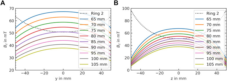
FIGURE 3. Optimization procedure of the base magnet to determine the optimal distance between the rings. Simulations of the magnetic flux densities of Ring 1 and 3 based on the distance between the rings (d1 in Panel 1F) along (A) y-direction and (B) z-direction. The magnetic flux distribution from Ring 2 (central ring) is plotted as a black dotted line. The concave curvature generated by the Ring 1 and Ring 3 configuration can be compensated to some extent by the convex curvature of Ring 2 in order to homogenize B_z.

Genetic Algorithm

For B₀-shimming, shim magnet placement was restricted in between and at the end of the base magnet rings (Figure 4), thus not reducing inner bore diameter or increasing the outer magnet dimensions. Furthermore, as the magnetic field decreases with the power of three Eq. (1), placing shim magnets further away from the targeted field of view increases the magnetic mass of the shims and the overall magnet weight and costs.

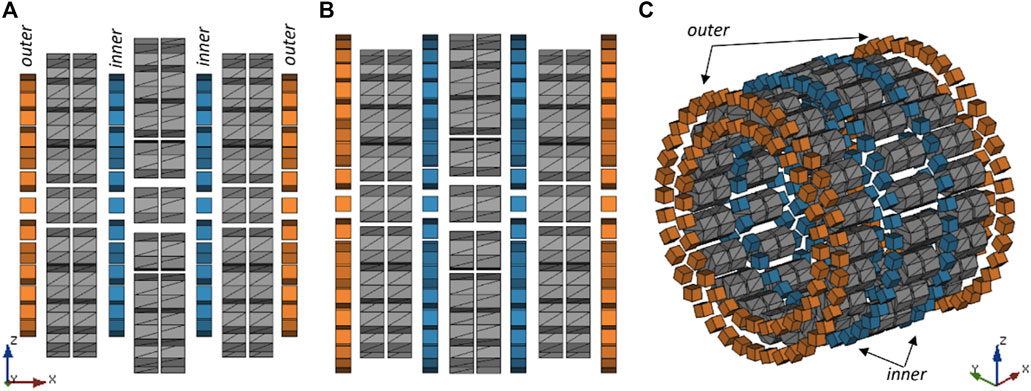
FIGURE 4. Illustration of the shim ring positions with respect to the base magnet (A) Side view of the shim ring positions with respect to the base magnet rings 1–3 (grey). Smallest radius rings of the inner (blue) and outer (orange) shim rings (for 9 mm magnet size the radius is 73 mm), (B) Sideview of the shim ring positions of the larger radius (r = 95 mm) for the inner and outer shim rings. (C) 3D view of the fully assembled magnet and position of the stacked shim rings with respect to the base magnet.

After B₀ field measurements to determine the B₀ field distribution of the base magnet in the field of view, a genetic algorithm is used to determine the size, position, and orientation of the shim magnets [9, 28]. Over other algorithms typically used in shimming as linear programming or the least square method this allows for a more flexible mathematical formulation of the optimization problem [29].

In the algorithm, a population (i.e., a collection of possible arrangements of shimming magnets) is evolved to find the best individual (i.e., best arrangement to homogenize the field). Each individual has a genome composed of genes (e.g., location of a shim magnet) describing the state (e.g., the orientation of the shim magnet) of the individual. As an underlying symmetry, the magnets are placed in a ring around the bore in Halbach or radial orientation. In total for each magnet five states were considered, four rotational deviations by 0°, 90°, 180° and 270° from the Halbach or respectively radial arrangement and the fifth state indicated no magnet placement.

The algorithm starts by creating 25,000 random individuals and calculates their cost function, which is a measure of inhomogeneity created by a given individual. The best individuals of the population are selected via tournament selection, where three individuals are chosen by random and the best is selected as a surviving individual. This process is repeated until the new population reaches the initial population size including redundant individuals. In the next step, the two-point crossover is performed with a probability of 75%, which recombines two neighbouring individuals by interchanging one randomly chosen part of their genome. To further diversify the population, a 20% mutation chance was set. If an individual mutates, every gene of its genome is changed randomly with a 5% chance. All cost functions, which have been changed by previous procedures, are calculated and the algorithm starts again with the tournament selection. The chosen probabilities have been shown to work well within the class of problems [8, 10]. A minimum of 300 iterations is performed, the algorithm converges when the last 20% of iterations do not create new individuals with a lower cost function. For the implementation, Python 3.6 was used and the DEAP module [9].

For the target field approach, using predetermined values at given spatial positions [30], the cost function is set to the peak-to-peak B₀ difference in the investigated 2D or 3D area. Compared to inhomogeneity, this avoids calculating the mean, which is numerically costly. This is reasonable since the B₀ shim field does not change the mean field amplitude significantly.

In addition, a representation based on spherical harmonics was investigated and the results compared to the target field approach. For this spherical harmonics approach, the cost function is chosen as the sum of the absolute values of the spherical harmonic coefficients (except the 0^th) [31, 32]. As orthonormalized functions are used, every function contributes equally to the field inhomogeneities and no weights are applied.

2D/3D B₀-Shimming

Prior to shimming the base magnet, simulations were performed to evaluate different shim configurations. The field of the magnet is simulated using the FEM and the genetic algorithm is used to assess different shimming scenarios. The number of magnets in one ring is maximized for the given radius while considering a 2 mm distance between neighbouring magnets. A single shim ring consists of two stacked rings of magnets with $r_1=67 mm+\frac{\sqrt{2}}{2}\cdot d_m$ (Figure 4A) and $r_2=95 mm$ (Figure 4B), where d_m is the magnet size. Three configurations were assessed:

1. One shim ring is positioned in between Ring 1 and Ring 2 and another one in between Ring 2 and Ring 3 with an offset of 26.25 mm from the center of the magnet. These rings are referred to as inner shim rings (Figure 4A).

2. One shim ring is placed in front of Ring 1 and another one at the end of Ring 3. These rings are referred to as outer shim rings (Figures 4A–C). The distance of the outer shim rings to the center of the bore is ±78.75 mm.

3. A combination of inner and outer rings, which is referred to as both.

For all these combinations, the genetic algorithm was applied for cube-shaped shim magnets of 6, 8, 10, 12 and 14 mm edge length. Two targets to homogenize the field were investigated:

1) A 2D area of 4 cm in diameter in y-z plane at the center of the magnet (x = 0), which corresponds to a 2D slice used for imaging

2) A 3D spherical volume of 4 cm in diameter around the center of the magnet.

Each simulation took on average 2 h 35 min with a standard deviation of 43 min on an Intel Xeon Processors E5-2,690 v3 (12 cores, 24 threads in total).

For the finally applied shims, cube shaped (9 × 9 × 9) mm³ NdFeB magnets (N48, Otom Group GmbH, Bräunlingen, Germany) were purchased. Before installation, the magnetic field of these magnets was measured at a distance of 45.6 mm to reduce variability in between magnets. Each 10th measurement a reference magnet was used, and the temperature was monitored (Figure 5). Magnets with stronger variations in magnetic field were sorted out. Within the errors of the sensor, they are normally distributed with a mean of 1.587 mT and a standard deviation of 7 μT. This results in a mean effective remanence (assuming a perfect magnet volume of (9 × 9 × 9) mm³) of 1.296 T with standard deviation 6 mT at 20°C. This mean remanence was used for the B₀ shimming calculations.

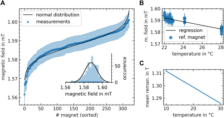
FIGURE 5. Experimental characterization of individual shim magnets used for populating the shim inserts. (A) Magnetic field measurements for each individual magnet represented by a blue dot. The error is displayed with an opaque blue band. In the inset, a histogram of the distribution of the magnetic field amplitudes is displayed. Quantification of the effective remanence of the shim magnets. (B) Magnetic field measurements of the reference magnet at different temperatures with regression fit to determine the temperature coefficient of the magnet. (C) Resulting temperature dependence of the mean effective remanence of all magnets calculated based on the temperature coefficient of the reference magnet.

Magnet Construction

The base magnet casing and the shim inserts were designed in FreeCAD (v018, http://www.freecadweb.org). Selective laser sintering (SLS), with a dimensional accuracy of ±0.3 mm, was used to fabricate the designs. These rings are positioned on four threaded brass rods, whereas the distance between the rings was adjusted using nuts (Figure 2D). Each shim ring consists of four interlockable pieces (Figures 2A–C), which can be inserted radially into the base magnet without modifying its assembly (Figure 2D). These shim inserts contain pockets that allow the placement of (9 × 9 × 9) mm³ magnets to be positioned at various angles in radial or Halbach orientation. A maximum of 76 shim magnets can be placed in a single shim ring, leading to an overall maximum of 304 shim magnets that can be inserted into the shims.

Measurement Setup

For magnetic field measurements of B_z, a Hallprobe (Gaussmeter Model 460, LakeShore Cryotronics, Westerville, OH, United States) was used. The Hallprobe was mounted to COSI Measure [33], an open source 3-axis positioning system with submillimeter precision, to autonomously map the magnetic field of the magnet before and after shimming. Since the magnets are temperature dependent, room temperature was measured inside a water bottle using a temperature probe (P550, Dostmann electronic GmbH, Wertheim-Reicholzheim, Germany). The 2D magnetic field measurements were performed at 1 mm spatial resolution in all dimensions inside an area/region of 5 cm diameter around the center of the bore. A snail shell like pattern was sampled (starting at the inside and moving towards the outside) with an overall measurement time of about 80 min. The 3D sphere was sampled on 40 evenly spaced points along the azimuthal plane and 40 points along the altitude angle obeying the quadrature points. This measurement took 70 min to sample 1600 points.

Results

Base Magnet

The distance d₁ between Ring 1 and Ring 3 was adjusted in measurements to 75 mm, which was the distance found giving the best compromise between compact magnet size and B₀ field homogeneity. The measured unshimmed magnetic field of the base magnet in the center of the field of view is B₀ = 102.8 (3) mT, with an inhomogeneity of 5,448 ppm in the 2D and 8,271 ppm in the 3D target region, both of 4 cm diameter.

B₀-Shimming

The results based on the simulations of the base magnet to evaluate the shim magnet size and configuration are displayed in Figure 6. For the 2D target the lowest B₀ inhomogeneity was 418 ppm using 10 mm magnets for the outer shim rings (Figure 6A). Using only the inner rings for shimming, the minimum was found for 9 mm cube magnets with an overall inhomogeneity of 1,240 ppm. A combination of inner and outer same sized magnets showed a minimum of 429 ppm using 9 mm cube shaped magnets. Like the 2D shimming results, 10 mm magnets showed the best homogeneity for the outer ring magnets with 4,015 ppm and a 3D target volume (Figure 6B). The magnet size for the inner ring magnets was best for 12 mm sized magnets with 4,091 ppm. Using the configuration “both” for same sized magnets, B₀ homogeneity could be improved slightly to 3,913 ppm for 9 mm magnets.

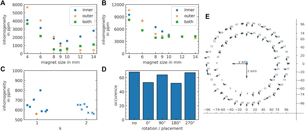
FIGURE 6. Results calculated by the shimming algorithms. (A) Homogeneities achieved for different shim magnet sizes based on the simulated magnetic field distribution (FEM) for configurations inner (blue circles), outer (orange crosses), both (green boxes) for (A) the 2D target slice of 4 cm in diameter and (B) the 3D sphere of 4 cm in diameter. (C) Calculated B₀ homogeneities for a radial (k = 1) and Halbach (k = 2) base symmetry of the shim. The best calculation is indicated in orange. (D) Occurrence of the rotational orientation and placement for the best design identified in C. (E) Example configuration of shim magnet placement in one shim ring. The arrows indicate the orientations of the magnetic moments at the respective positions of the shim magnets.

2D B₀-Shimming of the Base Magnet

Based on the simulation results, 9 mm cube shaped magnets were used to determine the shims for the base magnet. The results of the genetic algorithm for multiple runs and different magnet orientations [k = 1 (radial), k = 2 (Halbach)] are depicted in Figure 6C. Both show similar performance. Due to an easier construction process, a radial orientation was used for the final shim. The overall number of magnets at a certain rotational angle is displayed in Figure 6D and shows a balanced distribution between the different states. Overall, 236 of possible 304 magnets were placed in the shim rings and all rotational possibilities were used in the final set of shim magnets. The final shim magnet arrangement (exemplified on a single shim ring) is shown in Figure 6E. Implementing this shim, the simulations predicted a reduction in inhomogeneity by a factor 8 from 5,448 ppm (Figure 7A) to 560 ppm (Figure 7B). The measured field inhomogeneity was 682 ppm (Figure 7C). The calculated and measured field inhomogeneities over the target area are depicted in Figure 7D. A slight shift in the measured mean field was observed, which was 0.35 mT higher in the absolute B₀ values for the calculated shim configuration (Figure 7E).

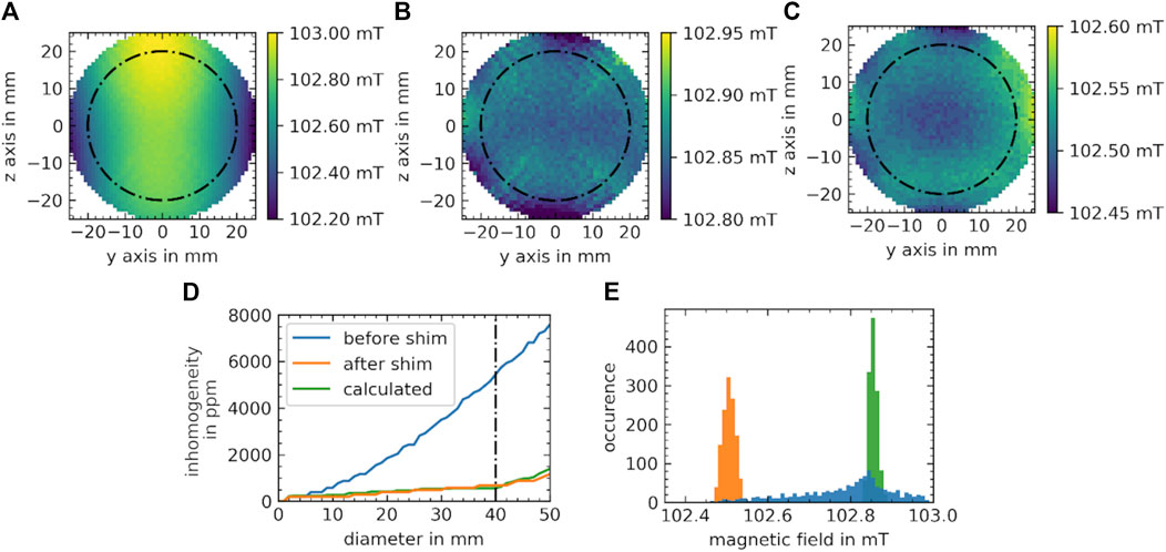
FIGURE 7. Measured magnetic field distributions before and after shimming on a two-dimensional target slice. (A) Measured field distribution of the desktop MR magnet before shimming. (B) Predicted distribution calculated by the genetic algorithm with the dipole approximation. (C) Measurement after the implementation of the shim. The black dash-dotted line indicates the 4 cm target region. (D) Field inhomogeneities over diameter of the slice measured before (blue) and after the shim (orange), together with the prediction of the shim, as calculated by the algorithm (green). (E) Occurrence of field values measured before (blue) and after shimming (orange) and calculated (green) by the algorithm in the 4 cm target area (dash-dotted line in D) using the same colour representation as in D.

Spherical Harmonics

All spherical harmonics coefficients up to the 17th degree and ±17th order of the measured B₀ field of the desktop magnet are shown in Figure 8A. To determine how many coefficients are necessary to properly reconstruct the field, the pointwise difference for a truncation at a certain degree (and order in the inset) is depicted in Figure 8B. Above degree four and order two no improvement (deviation <100 µT) of the reconstruction from the measured field can be observed. The difference between the measured (Figure 8C) and the reconstructed field based on the truncated ($l\le 4, m\le 4)$ spherical harmonics (Figure 8D) is depicted in Figure 8E. Overall a mean difference of 0.2 ± 17 µT was found with a maximum peak-to-peak difference of 145 μT in the overall volume. Consequently, the truncated spherical harmonics representation can be used to calculate a B₀ shim for the 3D volume, which reduced computational time substantially in particular for a larger number of shimming magnets.

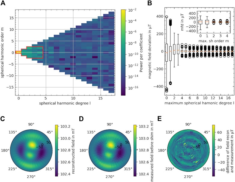
FIGURE 8. Evaluation of the measured magnetic field distribution on the 4 cm 3D sphere of the base magnet. (A) Power per spherical harmonic coefficient of the measurement. In red the truncated spherical harmonic coefficients are enclosed. (B) Boxplot of the point wise difference between the measured data and the reconstruction truncated at a maximum spherical harmonic degree. In the inset, the point wise difference for a maximum spherical harmonic order is displayed for the truncated spherical harmonics at degree four. The box extends from the lower to the upper quartile, the orange line represents the median and the whiskers extend according to Tukey’s boxplot. Outliers are indicated as circles. (C) Reconstruction of the measured field of the unshimmed desktop magnet with the truncated coefficients displayed in the red box in A. The field is displayed in polar projection, with the center of the depiction being at the greatest x coordinate. (D) Measured field without reconstruction. (E) Residuum of reconstruction and measurement.

3D B₀-Shimming

The calculated and measured 3D shim results are displayed in Figure 9. Before shimming, the 3D target sphere showed an inhomogeneity of 8,271 ppm. The calculated magnetic field distribution after shimming using the 9 mm magnets showed a inhomogeneity of 2,596 ppm (Figure 9A) over the target volume while the measured values were at 3,759 ppm (Figure 9B). The difference is displayed in Figure 9C. For the 3D approach, the improvement in homogeneity is less pronounced compared to the 2D target by only a factor of 2.2 (Table 1). Illustrating the shimming results based on spherical harmonic degree showed that all spherical harmonic coefficients except the coefficients of degree four can be shimmed efficiently (Figure 9D). Three coefficients are mainly contributing to the inhomogeneities. These are (l, m) = (2, −2), (l, m) = (4, 0) and (l) = (4, 2) as illustrated in Figure 9E. To further understand how the truncation of the field distribution is influencing the outcome of the shim, the field of the shim magnets is calculated with the dipole approximation and added to the truncated measured field before shimming. Compared to the calculation of the shim field with the truncated coefficients, the inhomogeneity reduces by 31 ppm. Consequently, the truncation of the dipole field of the shims is a good approximation and does not induce a large error. The results of the inhomogeneity per diameter of the sphere is displayed in Figure 9F. After a diameter of around 30 mm, B₀ inhomogeneity rapidly decreases.

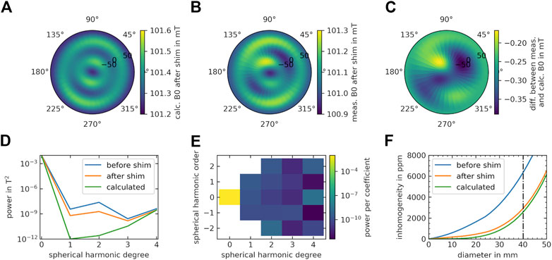
FIGURE 9. Measured field distribution after shimming for a 3D target sphere. The magnetic field distribution is depicted in polar projection of the field. (A) Calculated field distribution after the shim determined by the genetic algorithm with the dipole approximation. (B) Measured field distribution after the shim. (C) Difference between the measured and predicted data. (D) Power per spherical harmonic degree present in the unshimmed desktop magnet (blue) and determined after the shim by measurement (orange) and by calculation with the genetic algorithm (green). (E) Power per spherical harmonic coefficient for the measured field after shimming. (F) Field inhomogeneity in the target region of the desktop MR magnet. The data is reconstructed from field data measured on a 4 cm sphere using truncated spherical harmonics and plotted along the diameter of the three-dimensional sphere for the unshimmed (blue), shimmed (orange) magnet and predicted by the algorithm (green). The dash-dotted line indicates the diameter of the measured target region.

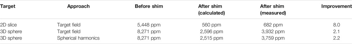
TABLE 1. Summary of 2D and 3D shimming results using the target field or spherical harmonics approach and the genetic algorithm.

Discussion

In this work, B₀ shimming based methodology is investigated to construct a homogeneous, low-cost and low-field (B₀ = 0.1 T) MR magnet using permanent magnets in an Halbach array configuration. The desktop magnet can be easily constructed using 3D printers, readily available NdFeB magnets and simple tools. It is relatively lightweight (∼15 kg) and has an overall material cost of ∼700 €, which is mostly due to the cost of the magnetic material used. It is therefore suitable to be used for educational applications in tabletop systems [21, 34] or small volume imaging applications.

Previous work demonstrated that a homogeneity of 2,400 ppm over the target field of view is sufficient to achieve good image quality at 50 mT using turbo spin echo sequences with reasonable acquisition times [9, 14, 15]. To reach these homogeneities for the desktop magnet, an iterative approach is suggested to build a base magnet that mainly determines the targeted B₀ field and in a second step to iteratively position shim inserts to improve the field homogeneity. With this approach, the initial B₀-field inhomogeneity of the base magnet of 5,448 ppm in the 2D area could be reduced by a factor ∼8–682 ppm in the first shimming iteration. The results are encouraging and suggest that even higher B₀ shimming homogeneities can be reached using an iterative approach. Simulation results of varying the shim magnet sizes show that the outer rings alone already improve B₀ field homogeneity substantially (Figure 6A). Consequently, a first shimming stage would e.g., implement the outer shim rings first and apply the genetic algorithm to determine the magnet size for the second shimming stage. Due to the more homogeneous base field, the magnets from the second stage will be much smaller (e.g., half the size) allowing space for the potential placement of another two shim rings in a third shimming stage close to the magnet center. This iterative shimming approach was not tested in this work due to limitations in the available Hall sensor sensitivity (∼500 ppm), which is clearly visible in the presented data (Figures 7B,C). For further investigations and to improve the results, a Hall sensor with higher sensitivity is needed or an NMR based magnetic field measurement where accuracies typically are in the order of 10 ppm or less.

For the 3D shimming results the target sphere could be shimmed from initially 8,271 to 3,759 ppm. This corresponds to an improvement by a factor of 2.2. Even though such improvement is comparable to other works on passive B₀ shimming after a single iteration [35], it is relatively low compared to the 2D shim results. Calculations based on the measured spherical harmonic coefficients (Figure 9F) demonstrated that B₀ field inhomogeneity decreases rapidly after around 30 mm diameter from the center of Ring 2. Further calculations (Figure 9D) showed that the main contributor to these inhomogeneities are the spherical harmonic coefficients of fourth degree, which could not be shimmed efficiently using the investigated setup. This indicates a drawback in the presented magnet design of the base magnet, which is adjusted to perform 2D imaging of a central slice. To improve the homogeneity along the x-axis, more rings are needed in order to approach the homogeneity of a perfect Halbach cylinder [26, 36]. Adding these rings however would furthermore increase the size, weight and cost of the magnet substantially and would require numerical optimization [36].

One advantage of the presented approach is that the shims can be inserted after the base magnet assembly, without compromising the inner or outer dimensions of the magnet. Placing movable magnet blocks inside the magnet [37], could further improve B₀ field homogeneity while compromising inner bore diameter. Placing shims outside of the magnet may require bigger shimming magnets and more magnetic mass. Another advantage of the three-ring setup for the base magnet is that, in principle, it can be constructed without any magnetostatic field simulations using FEM, where dedicated software is required. The distance adjustment between Ring 1 and Ring 3 can be performed based on the measurements alone. At this stage the optimization for homogeneity is less important due to the possibility of adding the shim inserts afterwards and homogenizing B₀ in an iterative manner using the genetic algorithm and the dipole approximation. This would allow the magnets to be scaled easily to a particular application of interest where a target B₀ is chosen based on parameters such as inner/outer radius and/or cost of magnetic material used [38]. Bigger magnet sizes are likely to further improve the shimming results since more shimming magnets can be used and magnetic field fluctuations in the target area due to position, orientation and/or material errors of individual shim magnets are expected to be less severe.

Octagonal magnets were used to improve the homogeneity of the base magnet and increase the magnetic flux compared to rectangular magnets [16, 27]. However, the first shim iteration is already improving homogeneity by nearly an order of magnitude, so it might be advantageous to use rectangular magnets, which are more accessible and affordable.

The calculations based on the genetic algorithm converged within 300 ppm (Figure 7D), therefore the parameters are chosen well and conservative. For 3D shimming and larger overall MR magnet dimensions the number of shim magnets that could be placed would increase together with the overall calculation time. Using the spherical harmonics approach investigated in this work reduces the number of parameters used for the genetic algorithm leading to a reduction in simulation time by a factor of ∼3.

From the data presented in Figure 7E, it is visible that the shimmed field shows lower overall B₀ values compared to the calculated shim. This may indicate a slight misalignment of the shim rings along the x-axis, which reduces the absolute field values in the target area. Improving the precision in aligning the shim rings along the x-axis may improve the shimming results in the y-z plane leading to values closer to the calculated ones.

A drawback of permanent magnets is the associated temperature drift of the magnetic field (Figure 5). In order to investigate the temperature dependence of B₀ field distribution of the current setup an additional experiment was performed, where the magnet was heated inhomogeneously (Supplementary Figure 1). This resembles a possible worst-case scenario, where both ambient temperature changes and local temperature changes are present. Heating the magnet to temperatures from 30.5–36.8°C resulted in a decrease in homogeneity from 407 to 1,095 ppm in the investigated area. Apart from the inhomogeneous temperature distribution which influences both base magnet and shim ring field drifts, a reason for the increased inhomogeneity at different temperatures might be the use of two different magnet grades used in the setup: N50 for the octagonal magnets and N42 for the shim inserts. Ideally a single material grade is implemented for both base magnet and shim inserts to avoid different temperature dependencies, which may affect B₀ homogeneity even for global temperature changes. An interesting approach to stabilize the field at different temperatures is the use of at least two magnetic materials with different temperature coefficients, which can be positioned in a way to cancel temperature dependent field variations efficiently [39]. Another way to counteract unavoidable temperature changes and homogenize the field is the use of active B₀ shimming techniques [31, 40].

Conclusion

It was demonstrated that an iterative approach to construct a cost-effective, homogeneous desktop MR magnet consisting of a base magnet and B₀ shim ring inserts is feasible. The approach is scalable to bigger magnet dimensions and has the potential to improve B₀ field homogeneity even further. These findings are encouraging towards increasing the availability of MR imaging technology globally using affordable low-field MR systems.

Data Availability Statement

The raw data supporting the conclusions of this article will be made available by the authors, without undue reservation.

Author Contributions

KW and LW contributed to conception and design of the study. KW, HA, and LW constructed the magnet. KW, HA, BS, and LW performed the measurements. KW and TO implemented the genetic algorithm. KW and LR implemented the spherical harmonics approach. KW and LW wrote the manuscript. All authors contributed to manuscript revision, read, and approved the submitted version.

Conflict of Interest

The authors declare that the research was conducted in the absence of any commercial or financial relationships that could be construed as a potential conflict of interest.

Publisher’s Note

All claims expressed in this article are solely those of the authors and do not necessarily represent those of their affiliated organizations, or those of the publisher, the editors and the reviewers. Any product that may be evaluated in this article, or claim that may be made by its manufacturer, is not guaranteed or endorsed by the publisher.

Acknowledgments

The authors would like to acknowledge Peter Blümler, Antonia Barghoorn, Raphael Moritz and Eva Behrens for their support.

Supplementary Material

The Supplementary Material for this article can be found online at: https://www.frontiersin.org/articles/10.3389/fphy.2021.704566/full#supplementary-material

Supplementary Figure 1 | Temperature dependent 2D B₀ field maps at the center of the magnet measured with an NMR probe (PT2026, Metrolab Technology SA, Geneva, Switzerland). The magnet was heated from a homogeneous baseline room temperature of 24.7°C to an inhomogeneous temperature distribution of 36.8°C on one outer shim ring vs. 30.5°C on the other outer shim ring. (A) Measured B₀ at 24.7°C room temperature with a mean of 91.58 mT and an inhomogeneity of 407 ppm. (B) B₀ field measurements for an inhomogeneous temperature gradient ranging from 30.5 to 36.8°C over the desktop MR magnet. Temperatures were measured with an infrared thermometer. The mean of the corresponding magnetic field is 1.15 mT smaller with 90.43 mT with an inhomogeneity of 1,095 ppm. C) Difference map between (A) and (B).

References

1.WHO | World Health Organization. Available from: http://gamapserver.who.int/gho/interactive_charts/health_technologies/medical_equipment/atlas.html (Accessed May 3, 2021).
2. Sarracanie M, Salameh N. Low-Field MRI: How Low Can We Go? A Fresh View on an Old Debate. Front Phys (2020) 8:172. doi:10.3389/fphy.2020.00172
3. Winter L, Pellicer-Guridi R, Broche L, Winkler SA, Reimann HM, Han H, et al. Open Source Medical Devices for Innovation, Education and Global Health: Case Study of Open Source Magnetic Resonance Imaging. Co-Creation (2019) 147–63. doi:10.1007/978-3-319-97788-1_12
4. Wald LL, McDaniel PC, Witzel T, Stockmann JP, Cooley CZ. Low-Cost and Portable MRI. J Magn Reson Imaging (2020) 52:686–96. doi:10.1002/jmri.26942
5. Marques JP, Simonis FFJ, Webb AG. Low-Field MRI: An MR Physics Perspective. J Magn Reson Imaging (2019) 49:1528–42. doi:10.1002/jmri.26637
6. Shah J, Cahn B, By S. Portable, Bedside, Low-Field Magnetic Resonance Imaging in an Intensive Care Setting for Intracranial Hemorrhage. Neurology (2020) 94:270.
7. Cooley CZ, McDaniel PC, Stockmann JP, Srinivas SA, Cauley SF, Śliwiak M, et al. A Portable Scanner for Magnetic Resonance Imaging of the Brain. Nat Biomed Eng (2020) 5:229–39. doi:10.1038/s41551-020-00641-5
8. Soltner H, Blümler P. Dipolar Halbach Magnet Stacks Made from Identically Shaped Permanent Magnets for Magnetic Resonance. Concepts Magn Reson (2010) 36A:211–22. doi:10.1002/cmr.a.20165
9. O’Reilly T, Teeuwisse WM, Webb AG. Three-Dimensional MRI in a Homogenous 27 cm Diameter Bore Halbach Array Magnet. J Magn Reson (2019) 307:106578. doi:10.1016/j.jmr.2019.106578
10. Cooley CZ, Stockmann JP, Armstrong BD, Sarracanie M, Lev MH, Rosen MS, et al. Two-dimensional Imaging in a Lightweight Portable MRI Scanner without Gradient Coils. Magn Reson Med (2015) 73:872–83. doi:10.1002/mrm.25147
11. Cooley CZ, Haskell MW, Cauley SF, Sappo C, Lapierre CD, Ha CG, et al. Design of Sparse Halbach Magnet Arrays for Portable MRI Using a Genetic Algorithm. IEEE Trans Magn (2018) 54:1–12. doi:10.1109/TMAG.2017.2751001
12. McDaniel PC, Cooley CZ, Stockmann JP, Wald LL. The MR Cap: A Single-Sided MRI System Designed for Potential Point-of-Care Limited Field-Of-View Brain Imaging. Magn Reson Med (2019) 82:1946–60. doi:10.1002/mrm.27861
13. Vogel MW, Guridi RP, Su J, Vegh V, Reutens DC. 3D-Spatial Encoding With Permanent Magnets for Ultra-low Field Magnetic Resonance Imaging. Sci Rep (2019) 9:1522. doi:10.1038/s41598-018-37953-1
14. O’Reilly T, Teeuwisse WM, Gans Dde, Koolstra K, Webb AG. In Vivo 3D Brain and Extremity MRI at 50 mT Using a Permanent Magnet Halbach Array. Magn Reson Med (2021) 85:495–505. doi:10.1002/mrm.28396
15. Van Speybroeck CDE, O'Reilly T, Teeuwisse W, Arnold PM, Webb AG. Characterization of Displacement Forces and Image Artifacts in the Presence of Passive Medical Implants in Low-Field (<100 mT) Permanent Magnet-Based MRI Systems, and Comparisons With Clinical MRI Systems. Physica Med (2021) 84:116–24. doi:10.1016/j.ejmp.2021.04.003
16. Blümler P, Casanova F. CHAPTER 5. Hardware Developments: Halbach Magnet Arrays. In: ML Johns, EO Fridjonsson, SJ Vogt, and A Haber, editors. New Developments in NMR. Cambridge: Royal Society of Chemistry (2015). p. 133–57. doi:10.1039/9781782628095-00133
17. O’Reilly T, Webb AG. The Role of Non-Random Magnet Rotations on Main Field Homogeneity of Permanent Magnet Assemblies. Proc Intl Soc Mag Reson Med (2021) 4042.
18. Lopez HS, Liu F, Weber E, Crozier S. Passive Shim Design and a Shimming Approach for Biplanar Permanent Magnetic Resonance Imaging Magnets. IEEE Trans Magn (2008) 44:394–402. doi:10.1109/TMAG.2007.914770
19. Überrück T, Blümich B. Variable Magnet Arrays to Passively Shim Compact Permanent-Yoke Magnets. J Magn Reson (2019) 298:77–84. doi:10.1016/j.jmr.2018.11.011
20. Parker AJ, Zia W, Rehorn CWG, Blümich B. Shimming Halbach Magnets Utilizing Genetic Algorithms to Profit from Material Imperfections. J Magn Reson (2016) 265:83–9. doi:10.1016/j.jmr.2016.01.014
21. Cooley CZ, Stockmann JP, Witzel T, LaPierre C, Mareyam A, Jia F, et al. Design and Implementation of a Low-Cost, Tabletop MRI Scanner for Education and Research Prototyping. J Magn Reson (2020) 310:106625. doi:10.1016/j.jmr.2019.106625
23. Chen J, Wang D, Cheng S. A Hysteresis Model Based on Linear Curves for NdFeB Permanent Magnet Considering Temperature Effects. IEEE Trans Magn (2017) 54:1–5. doi:10.1109/TMAG.2017.2763238
24. Wieczorek MA, Meschede M. SHTools: Tools for Working with Spherical Harmonics. Geochem Geophys Geosyst (2018) 19:2574–92. doi:10.1029/2018GC007529
25. Moritz R. Development and Characterization of Halbach Arrays Tailored for Magnetic Resonance at Low Magnetic Field Strengths. Berlin, Germany: MSc Thesis TU Berl (2017).
26. Raich H, Blümler P. Design and Construction of a Dipolar Halbach Array with a Homogeneous Field from Identical Bar Magnets: NMR Mandhalas. Concepts Magn Reson (2004) 23B:16–25. doi:10.1002/cmr.b.20018
27. Barghoorn A. Halbach Magnet Array Design for Low Cost Magnetic Resonance Imaging. Berlin, Germany: BSc Thesis TU Berl (2016).
29. Kong X, Zhu M, Xia L, Wang Q, Li Y, Zhu X, et al. Passive Shimming of a Superconducting Magnet Using the L1-Norm Regularized Least Square Algorithm. J Magn Reson (2016) 263:122–5. doi:10.1016/j.jmr.2015.11.019
30. Ye B, Wang Q, Yu Y, Kim K. Target Field Approach for Spherical Coordinates. IEEE Trans Appl Supercond (2004) 14:1317–21. doi:10.1109/TASC.2004.830565
31. Wachowicz K. Evaluation of Active and Passive Shimming in Magnetic Resonance Imaging. Res Rep Nucl Med (2014) 4:1–12. doi:10.2147/RRNM.S46526
32. Roméo F, Hoult DI. Magnet Field Profiling: Analysis and Correcting Coil Design. Magn Reson Med (1984) 1:44–65. doi:10.1002/mrm.1910010107
33. Han H, Moritz R, Oberacker E, Waiczies H, Niendorf T, Winter L. Open Source 3D Multipurpose Measurement System with Submillimetre Fidelity and First Application in Magnetic Resonance. Sci Rep (2017) 7:13452. doi:10.1038/s41598-017-13824-z
34.OCRA – Open-Source Console for Real-Time Acquisition. Available from: https://zeugmatographix.org/ocra/ (Accessed May 3, 2021).
35. Zhang Y, Xie D, Bai B, Yoon HS, Koh CS. A Novel Optimal Design Method of Passive Shimming for Permanent MRI Magnet. IEEE Trans Magn (2008) 44:1058–61. doi:10.1109/TMAG.2007.916267
36. Turek K, Liszkowski P. Magnetic Field Homogeneity Perturbations in Finite Halbach Dipole Magnets. J Magn Reson (2014) 238:52–62. doi:10.1016/j.jmr.2013.10.026
37. Danieli E, Mauler J, Perlo J, Blümich B, Casanova F. Mobile Sensor for High Resolution NMR Spectroscopy and Imaging. J Magn Reson (2009) 198:80–7. doi:10.1016/j.jmr.2009.01.022
38. Winter L, Barghoorn A, Blümler P, Niendorf T. COSI Magnet: Halbach Magnet and Halbach Gradient Designs for Open Source Low Cost MRI. Proc Intl Soc Mag Reson Med. (2016). p. 3568.
39. Danieli E, Perlo J, Blümich B, Casanova F. Highly Stable and Finely Tuned Magnetic Fields Generated by Permanent Magnet Assemblies. Phys Rev Lett (2013) 110:180801. doi:10.1103/PhysRevLett.110.180801
Keywords: magnetic resonance imaging, B0 shimming, low field MRI, Halbach arrays, MR magnet, open source hardware
Citation: Wenzel K, Alhamwey H, O’Reilly T, Riemann LT, Silemek B and Winter L (2021) B0-Shimming Methodology for Affordable and Compact Low-Field Magnetic Resonance Imaging Magnets. Front. Phys. 9:704566. doi: 10.3389/fphy.2021.704566
Received: 03 May 2021; Accepted: 09 July 2021;
Published: 28 July 2021.
Edited by:
Lionel Marc Broche, University of Aberdeen, United KingdomReviewed by:
Esteban Anoardo, Universidad Nacional de Córdoba, ArgentinaDuarte Mesquita Sousa, University of Lisbon, Portugal
Copyright © 2021 Wenzel, Alhamwey, O’Reilly, Riemann, Silemek and Winter. This is an open-access article distributed under the terms of the Creative Commons Attribution License (CC BY). The use, distribution or reproduction in other forums is permitted, provided the original author(s) and the copyright owner(s) are credited and that the original publication in this journal is cited, in accordance with accepted academic practice. No use, distribution or reproduction is permitted which does not comply with these terms.
*Correspondence: Lukas Winter, lukas.winter@ptb.de