
. Introduction
Loess areas are susceptible to soil erosion, especially when under agricultural land use. Loess areas in southern Poland have been used for agriculture since the Neolithic (Kruk et al, 1996, Kruk and Milisauskas, 1999). The advent of agriculture in this area resulted in changes of plant cover on the slopes, which increased their susceptibility to processes such as rainsplash, sheet erosion and linear erosion. Since the beginning of the Neolithic, these processes have intensified as human settlements have increased in size and number (Kruk et al, 1996; Starkel, 2005). Intensification of the soil erosion processes can be noticed from the Middle Ages until the present time, but for the last 50 years have reached their maximum (Śnieszko, 1995; Doterweich, 2008; Starkel, 2005). The accumulation of sediments at the foot of the slopes and in valley bottoms – to which the slopes episodically drain – provides a partial record of slope erosion (Śnieszko, 1991, 1995). I n t he case of small catchments in loess areas, soil erosion is associated rather with agricultural land use, while climate change is probably less important (Lang, 2003; Zolitschka et al, 2003; Fuchs et al, 2004; Zadorova et al, 2013).
The presence of sediments indicating both Neolithic and medieval water erosion of soil were observed as the infill relicts exposed in gully walls in the area where studies of modern soil erosion were carried out in the past (Śnieszko, 1995). The age of these colluvial sediments was documented by OSL dating. The aggradation of soil material eroded by water is synchronous with the archaeologically documented phases of agricultural colonization. The thickness of Holocene colluvial deposits accumulated in this area do not exceed 4 m. A comparison of these sediments resulting from soil erosion and characterized by limited thickness for the last 5–6 thousand years with the results of studies on the magnitude of contemporary soil erosion gives an idea of the difference in intensity of the erosion processes nowadays and in the past in this particular area (Śnieszko, 1985, 1987, 1995). One location where the impact of crop farming was significant for the natural environment in the past is near the Bronocice settlement in southern Poland. In the central part of the Nidzica Basin, one of the largest concentrations of funnel-bowl culture settlements was documented (Kruk et al, 1996). The settlement centre was located in the area of the contemporary village of Bronocice and was used by Neolithic farmers from 3900 BC to 2500 BC (Kruk et al, 2016). Numerous satellite settlements were also formed, which resulted in the water erosion of soils throughout the entire microregion (Kruk et al, 1996).
Archaeological investigation of this settlement and its neighbouring area has revealed no signs of agricultural pressure after the Neolithic until the Middle Ages, when settlements were established in locations where villages have persisted to this day (Kruk et al, 1996; Kruk and Milisauskas, 1999). Until now, only the results of radiocarbon dating of fossil soil humus lying at the base of the Holocene colluvial sediment wedge have provided a chronology for this accumulation (Kruk et al, 1996; Kruk and Milisauskas, 1999).
The precise determination of the intensity of soil erosion that occurs today, as well as from the past, is a vital problem in palaeoenvironmental studies and still requires intensive research. Moreover, the precise age of sediment formation plays an important role in modelling past environmental dynamics. Each land cover change on the slope due to ploughing produces accelerated soil erosion on the slope itself, and sediment accumulation within mid-slope flat areas and on valley floors (Zadorova et al, 2013). Reliable defining the time frame of accumulation of slope sediments is essential to estimate the impact of the evolving agricultural systems through time. To reconstruct the age of pre-historical and historical phases of soil erosion intensification, the OSL (optically stimulated luminescence) method provides a suitable tool. Luminescence dating typically refers to the time elapsed since the last exposure of some silicate minerals to daylight. The practical usefulness of this method has been discussed for this type of sediment in the review work published by Fuchs and Lang (2009). In the case of the recent soil erosion being investigated, For studies of soil erosion which took place during the last century, two radioisotopes are very useful; the artificial radioactive fallout of 137Cs (covering the period of the last 70 years) and the natural fallout of 210Pb (covering the period of the last 100–150 years) have been successfully applied (Walling and He, 1999; Mabit et al, 2008). Although 137Cs has been successfully used to study soil erosion, 210Pbex is relatively rarely used in such studies when compared to 137Cs. Instead, this method is most often used to study sedimentation rates in lakes, ponds or peat environments with a time depth of about 100–150 years (Mabit et al, 2014).
The objective of this research was to use radioactive fallout, OSL and dendrochronology to further explore the potential for combining those dating methods to document soil redistribution over different time scales and human impact on the study area. In this study, we present the results of soil erosion analysis using the 137Cs and 210Pbex methods, OSL dating, sediment analysis, micromorphology analysis and dendrochronology analysis. The soil erosion during the last 50–100 years was determined in ploughed land using both the 137Cs and 210Pbex methods. To extend the study beyond the recent sediments to the Holocene colluvial package, luminescence dating method was also employed, specifically, the OSL dating of coarse-sized grains (Fuchs and Lang, 2009). Those dating methods, in connection with pedological and sedimentological analysis, provide information about the age of pre-historical and historical phases of intensified soil erosion. Additionally, dendrochronological analyses in our studies was used, mainly for checking whether erosion processes are currently active in the under study gully. Tree ring analyses can provide information about evolution of the gully morphology in a wide range of time from the last few decades to the hundreds of years (depending on the sampled tree age); (Vandekerckhove et al, 2001; Malik, 2008). Different types of anatomical features are used for dating erosion events in forested gullies and valley floors, these are: reaction wood, eccentric tree growth, ring reductions, and decrease of cell size after root exposure (Gärtner et al, 2001; Malik, 2006a; Stoffel et al, 2012). Those anatomical features allow, for example, to reconstruct the rate of sheet and gully erosion, or to determine the patterns of gully formation, and sometimes estimate the time when erosion started (Bodoque et al, 2005; Malik, 2006b). Considering the proposed methods and scope of research, the presented approach in the paper allows to obtain reliable results to reconstruct the soil erosion and sediment accumulation dynamics in an area of great archaeological importance. Extensive archaeological studies show that this loess region belongs to heavily transformed loess areas under the influence of agricultural activity since the Neolithic (Kruk et al, 1996).
. Materials and methods
Investigated Sites
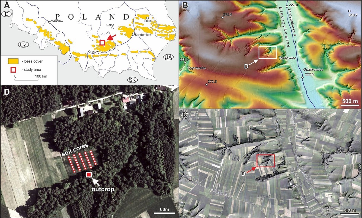
The study site is located near Biedrzykowice village (50°23'56.10"N; 20°18'44.26"E) in southern Poland, in the mesoregion named the Proszowice Plateau located on eastern part of the Małopolska Upland (Kondracki, 2002). (Figs. 1A–1D). The topographic surface of the Proszowice Plateau is situated between 220–390 m a .s.l., and the depth of the larger valleys ranges from 40 to 60 m. The mean slope inclination for a study plot is about 10°.
Fig. 1
A – Location of research area on the map of loess distribution (yellow patches) in southern Poland; B – DEM model; C – orthophotomap; D – aerial photo
The oldest rocks in the exposures are chalk marbles forming culminations. Miocene gypsum and clay occur under Quaternary formations. The cover of Pleistocene glacial formations has only been studied to a very limited degree. It consists of residual clays and sands of the oldest glaciation periods, whose stratigraphic affiliation is difficult to determine. Loess deposits are the most common Pleistocene sediments. Jersak (1973) assigned these areas to the transition loess formation. Here the loess cover can reach a thickness of 20 m and colluvial sediments on the footslope and toeslope as much as 7 m. The main part of the loess cover consists of the youngest Vistulian (=Weichselian) loess deposits accumulated mainly during younger part of MIS 2, i.e between 22 ka BP and 16 ka BP (e.g. Maruszczak, 1991, 2001; Jary, 2007).
Mean annual precipitation is 657 mm with the highest intensity in July. The mean value of July precipitation is 95 mm and the greatest recorded monthly precipitation (also recorded in July) was 226.1 mm (https://pl.climate-data.org/location/10413/#climate-graph) The average annual temperature is 8.2ºC, with a range from –4.4ºC (January) to 18.6ºC (July). The growing period is about 200 days of the year (Paszyński and Kluge, 1986). This area has been used as cultivated fields since the Neolithic (Kruk et al, 1996, 2016; Kruk and Milisauskas, 1999). Archaeological investigations in this area suggest a strong impact by farmers on the primary landscape in the years 3900–2500 cal. BC (Kruk et al, 1996, 2016). In Biedrzykowice, located almost 8 km north of the Neolithic site in Bronocice, a colluvial sediment profile preserved at the bottom of a dry valley (Sancygniówka River basin), which has been the subject of previous analyses (Śnieszko, 1985, 1995; Raven et al, 1999), was selected for detailed studies.
Sampling
Colluvial sediments and soil samples were collected from the wall of the gully as well as from the adjacent agricultural field (Fig. 1D). For the soil erosion and sedimentation study using fallout radionuclide, 34 cores were collected using a “Stiboka” motorized corer (inserting 10 cm diameter demountable steel tubes into the soil profiles) along five downslope transects from an agricultural field. The motorized sample corer allowed soil cores with a non-disturbed structure to be obtained. Core locations were recorded using an RTK GPS (Promark 220, about 0.1 m accuracy) and are presented in Fig. 1. The soil cores were sectioned into 10 cm intervals. Additional cores were collected from undisturbed reference sites and sectioned at 2, 3 or 5 cm increments. Reference sites were selected as places where soil erosion and sediment accumulation were not visible (mature and natural vegetation cover protects the soil surface from erosion). In the case of luminescence dating, two sets of samples were taken: the first from a gully wall and the second from an agricultural field close to the gully. We collected 13 samples for OSL dating and 50 samples for radionuclide analysis from the gully wall. The samples for optical dating were collected by using steel tubes driven into the sediment. The tubes were opened in a dark laboratory and about 1 cm of the sediment at each end was cut and removed before OSL measurement. Samples for activity measurement were taken from the surface to a depth of 500 cm. Samples for luminescence dating were also collected from three areas on the agricultural field: top of the slope, eroded area and base of the slope. This sampling was also performed using a light-protected procedure.
As well as the simultaneous application of both methods, 13 detailed micromorphological soil analyses were also carried out. The main goal of the micromorphological analyses was to determine litho- and pedological features (e.g. Kemp, 2001; Mroczek, 2008, 2013, 2018). The micromorphological samples were taken from the same horizons in the gully wall as the samples for OSL dating.
For dendrochronological analyses, we chose six larch trees (Larix decidua Mill.) growing on the edge of the gully under study. Due to erosion, the trees were tilted perpendicularly to the valley axis, and additionally their root system was partially exposed. We assumed that dendrochronological analyses would allow us to date erosion events and estimate the rate of gully hillslope retreat. Growth disturbances (tree ring reduction, tree ring eccentricity) formed after erosion events and recorded in wood of the studies trees were used to erosion dating. We collected two cores from each of the six trees with a Pressler borer at chest height, perpendicularly to the valley axis (6 cores) and parallel to the valley axis (6 cores). We also sampled by handsaw 4 exposed roots from tree number 6: root sample number 1 – sampled 5 cm from the gully edge, root sample number 2 – sampled 15 cm from the gully edge, root sample number 3 – sampled 20 cm from the gully edge, and root sample number 4 – sampled 50 cm from the gully edge. We assumed such a strategy would allow the rate of gully hillslope retreat to be checked.
Activity measurement
Before the activity measurement, all samples were dried, placed in measurement containers and stored for a minimum of three weeks to ensure radioactive equilibrium in the decay series. The activities of 137Cs and 210Pb, as well as other isotopes, such as the 238U series, 232Th series and 40K, were measured for dose rate determination by using low background high resolution gamma spectrometry analysis. The detector resolution (FWHM) was 1.8 keV and the relative efficiency was 40% at 1332 keV. The counting time was usually 8 0 ks and IAEA ( RGU, RGTh, RGK) standards were used for calibration. The IAEA Soil-375 standard was used as a reference material for 137Cs activity. The IAEA-385 standard was used to check the quality of efficiency calibration. To calculate the 238U content in the sediment, the following gamma lines were taken: 295.1 keV (214Pb), 352.0 keV (214Pb), 609.3 keV (214Bi) and 1120.3 keV (214Bi). For the 232Th decay chain, the following gamma lines were considered: 583.0 keV (208Tl), 911.2 keV (228Ac) and 2614.4 keV (208Tl). To calculate the 40K content, the 1460.8 keV gamma line was taken. To calculate the 137Cs content, the 661.7 keV gamma line was used. The total activity of210Pb in the samples was measured at 46.5 keV and the concentration of the supported 210Pb was assayed by measuring the short-lived daughters of 226Ra. The unsupported 210Pb activity (210Pbex ) in the samples was calculated by subtracting the supported 210Pb from the total concentration of 210Pb. In the case of 210Pb, the results were corrected for self-absorption, in accordance with Cutshall et al (1983).
Dose rate calculation
The measured activities of radioisotopes in the sediment and soil samples were converted into dose rates by using the conversion factors described by Guerin et al (2011). The dry dose rates (Adamiec and Aitken, 1998; Guerin et al, 2011) were adjusted for water content, following Aitken (1985). The water content of samples measured in the laboratory was no higher than 15%, so we used a value of 10 ± 5% for our calculations (Bluszcz, 2000). The cosmic ray dose-rate at the site follows the calculations suggested by Prescott and Hutton (1994).
The results of radionuclide analysis as results of dose rate calculation are summarized in Table 1. For the sediment samples, the dating of the 137Cs activity was included in the calculation of the dose rate, according to the procedure described in (Moska et al, 2004; Poręba et al, 2006).
Table 1
Results of activity concentration measurement (based on low-level semiconductor γ-spectrometry), dose rate calculation, De estimation and OSL ages for sediment samples from Biedrzykowice. 1Doses for samples collected from a depth lower than 50 cm were corrected with respect to range of gamma rays. 2Dose rates in this column were obtained by using portable gamma spectrometer in situ
137Cs and 210Pb dating
Caesium-137 (half-life 30.1 years) is a radioisotope whose main source in the environment is above-ground nuclear weapon tests in the 1950s and 1960s. The 137Cs fallout connected with nuclear weapon testing is known as global fallout, and its distribution depends on latitude and precipitation. The highest intensity of 137Cs deposition occurred in the period 1961–1963. Additionally, another 137Cs fallout connected with the Chernobyl accident of 1986 has taken place in Europe. 137Cs is strongly adsorbed into soil particles (Ritchie and McHenry, 1990) after its deposition on the ground surface, In areas contaminated as a result of the Chernobyl accident, calculation of soil erosion based on the 137Cs inventories can be difficult due to problems in distinguishing between global and Chernobyl 137Cs fallouts (Golosov et al, 1999; Poręba and Bluszcz, 2007). In contrast to 137Cs, 210Pb (with a half-life of 22.2 years) is a natural radioactive isotope which is a part of the 238U decay chain. This isotope is derived from the radioactive decay of 222Rn, a daughter of 226Ra. 210Pb produced from 226Ra in situ in soil is known as supported, whereas the 210Pb originating from atmospheric fallout is named unsupported (or 210Pbex), and is used widely to study the accumulation rates of various sediments. The activity of 210Pbex is usually calculated by subtracting the supported 210Pb established via the activity of the 226Ra daughters from the total 210Pb in a given soil or sediment sample (Walling, 1998; Walling and He, 1999; Mabit et al, 2014).
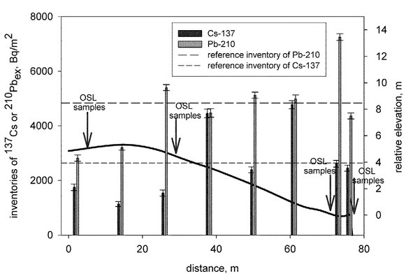
The measured 137Cs and 210Pbex activities were converted to inventories according to the formula described by Sutherland (1992) and are presented in Figs. 2–3. The simple comparison between the measured values of the 137Cs or 210Pbex inventories and the reference inventory values of 137Cs or 210Pbex allows us to recognize erosion and deposition areas; however, to obtain quantitative estimates of soil erosion, one of several available models must be used (Walling and Quine, 1990; Walling and He, 1999).To estimate soil erosion based on 137Cs and 210Pbex, the proportional model (137Cs) as well as two mass balance models (137Cs, 210Pbex) were applied (Walling and Quine, 1990; Walling and He, 1999; Poręba, 2006). The equation for the proportional model can be written as (Walling and Quine, 1990):
Fig. 2
The spatial patterns of 137Cs and 210Pbex inventories on the studied agricultural field. The data on the figure are expressed in Bq·m–2.
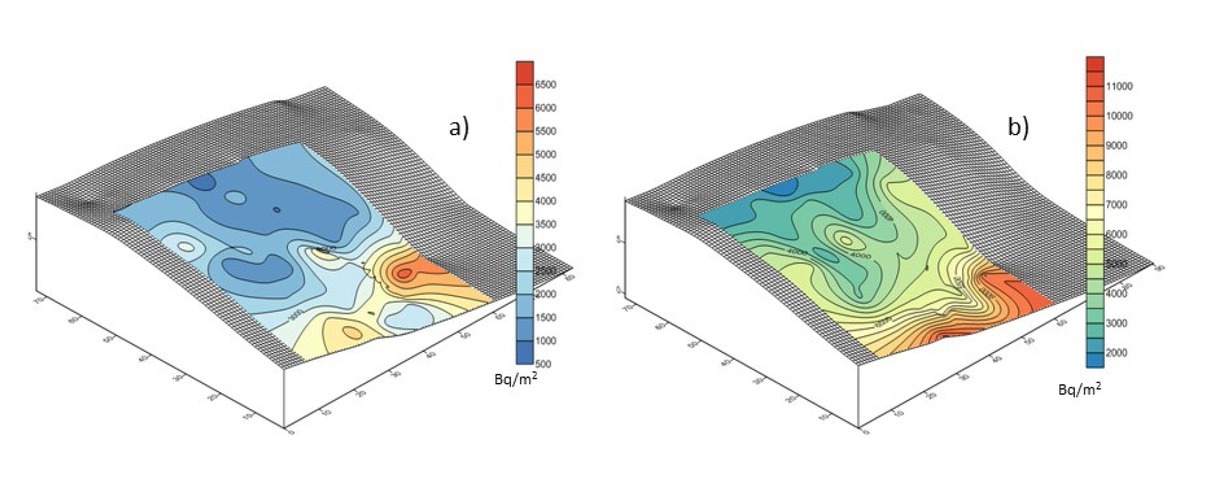
Fig. 3
The downslope change of 137Cs and 210Pbex inventories. On the figure is marked the shape of the slope.
where:
- Y – mean annual soil loss (t·ha–1·a–1),
- B – bulk density of the soil (kg·m–3),
- d – depth of the plough layer (m),
- X – percentage reduction in total 137Cs inventory (defined as (Aref - A)/Aref ·100),
- Aref – local 137Cs reference inventory (Bq·m–2),
- A – measured 137Cs inventory at the sampling point (Bq·m–2),
- T – time elapsed since initiation of 137Cs accumulation (a),
- P – the particle size correction factor (possible difference between the grain size composition of the mobilized sediment and the original soil). The value of this factor could be calculated according to He and Walling (1996).
The main assumption for the proportional model is that 137Cs is completely mixed within the plough layer. If this is true, then the soil loss is directly proportional to the 137Cs loss from the soil profile. Although this model is relatively easy to use, it has several limitations. For instance, this model assumes that caesium is uniformly distributed in the plough layer. Immediately after fallout, the surface contained more caesium than the underlying soil horizons due to agricultural mixing, e.g. ploughing. This could result in an overestimation of soil loss (Walling and Quine, 1990). Two kinds of mass balance models were also used to calculate soil erosion and deposition. The first mass balance model was described by Zhang et al (1990) and is referred to as the simplified mass balance model. The main assumption of this model is that the total 137Cs fallout occurred in 1963. The mean annual soil loss rate can be expressed as follows:
where:
- Y – mean annual soil loss (t·ha–1·yr–1),
- d – depth of the plough layer (m),
- B – bulk density of soil (kg·m–3),
- X – the percentage reduction in total 137Cs inventory (defined as (Aref – A)/Aref ·100),
- t – time since the year 1963.
Although this model is very easy to use, the main assumption of this approach that the total 137Cs fallout input occurred in 1963 seems to be an oversimplification. This model does not take into account the value of 137Cs freshly removed from the soil surface before incorporation into the plough layer by ploughing. The problem with selective sorption of 137Cs by soil particles could be solved by adding a particle size correction factor (Zhang et al, 1999). Another problem with the simplified mass balance model is the assumption of the 137Cs fallout in 1963. This does not take into account areas contaminated by Chernobyl caesium, such as the study area.
To overcome the problem with selective sorption, and also removing the fresh deposition of 137Cs before mixing by ploughing, the mass balance model was improved by He and Walling (1997). This model was also used to calculate soil erosion based on the 210Pbex inventories. According to He and Walling (1997), this model could be written as follows:
where:
- A(t) – cumulative 137Cs or 210Pbex activity per unit area (Bq·m–2),
- R – soil erosion rate (kg·m–2·a–1),
- d – the average plough depth (kg·m–2),
- λ – the radioactive decay constant for 137Cs or 210Pbex (a–1),
- I(t) – annual 137Cs or 210Pbex deposition flux (Bq·m–2 a–1),
- Γ – the percent of the fresh deposition of 137Cs or 210Pbex removed by erosion before mixing into the plough layer,
- P – the particle size correction factor (see footnotes for Eq. 2.1)
For the areas where deposition of soil occurs, the mass balance model could be written according to Walling and He (1999) to calculate the soil deposition rate:
where:
Luminescence dating
Samples for OSL dating were treated with 10% HCl and 10% H2O2 for 48 hours to remove carbonates and organic material, respectively. Quartz was extracted from the 90–125 μm grain fraction by using density separation (sodium polytungstate). Finally, quartz grains were etched using 40% HF to remove their outer layer (Aitken, 1985, 1998). After etching, they were washed in HCl (20%) to remove any precipitated fluorides. The grains were then mounted on stainless steel discs using silicone oil. All treatment was conducted under subdued red light.
Quartz from each sample was checked for purity by means of an I R-test. No samples showed a significant IRSL signal, i.e the natural and regenerated signal ratios of the IRSL to the blue-light stimulated luminescence were ≤ 5%. The SAR procedure which was used for equivalent dose determination did not contain IRSL step.
Optically stimulated luminescence measurements (OSL) were made using an automated Daybreak 2200 TL/OSL reader (Bortolot, 2000), equipped with a calibrated 90Sr/90Y beta source (dose rate of 2.95 ± 0.09 Gy·min–1).
The determination of equivalent doses of quartz grains was performed using multi-grain aliquots, each containing ca 1 mg of quartz grains. A 6 mm mask was used to disk preparation, it means that on the single disk should be about 1500 quartz grains with 90–125 μm diameter (Heer et al, 2012). For stimulation, blue diodes (470 ± 4 nm) delivering 45 mW·cm–2 at the sample position were used. Equivalent doses were determined using a single-aliquot regenerative-dose (SAR) protocol (Murray and Wintle, 2000). Dose recovery and thermal transfer tests were performed for each sample and a preheat plateau test was performed to establish the most appropriate preheat temperature.
Micromorphological analyses
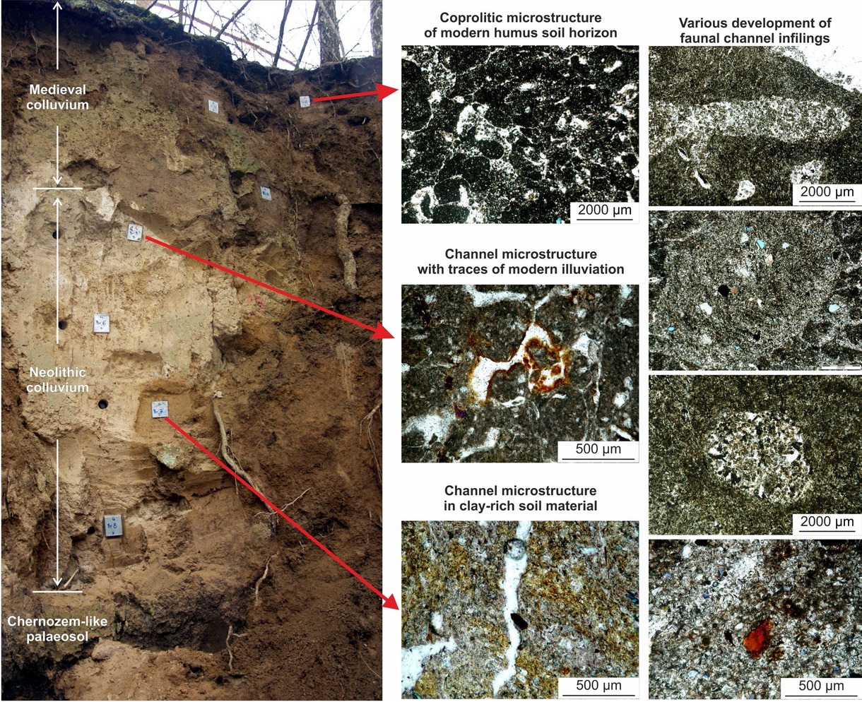
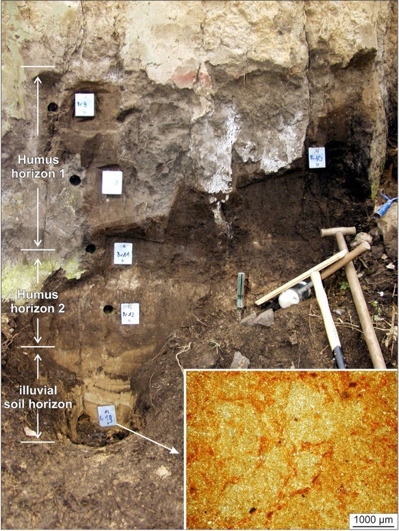
Micromorphological analyses were carried out on a selected sequence of colluvial sediments with intercalated palaeosoil horizons in the gully (Figs. 4–5). The micromorphological samples were taken from the same horizons in the vertical outcrop as the samples for OSL dating. The material was collected in Kubiena tins (8×6×4 cm) directly from selected colluvial layers and soil horizons. Thin sections were made of samples according to the methodology proposed by Lee and Kemp (1992) and modified by Mroczek (2008). The size of the individual thin sections was ~8×6 cm, and their thickness ranged from 20 to 30 μm. Thin sections were observed using a polarizing microscope with magnifications up to 200×.
Dendrochronology
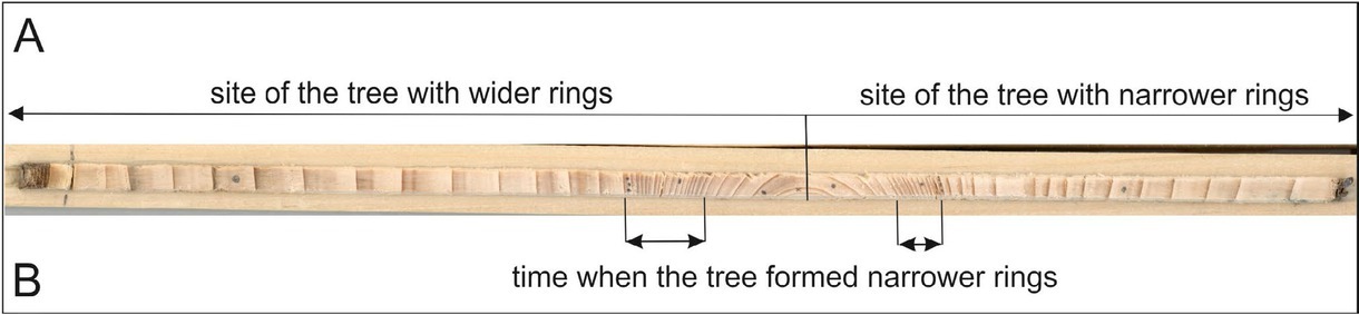
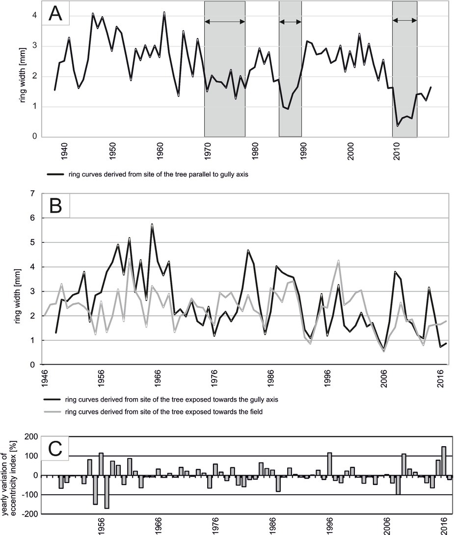
Within cores we dated the eccentric growth of trees, which is formed due to trees tilting and is relatively easy to observe in the wood cross-sections (Fig. 6A). We used cores collected perpendicularly to the gully axis for eccentric growth analyses. After root exposure, a tree produces reduced rings, therefore we also analysed ring reduction in the sample cores (Fig. 6B). The eccentric growth of trees develops on the side in which the tree stem is tilted (in the case of conifers), while ring reduction occurs on the entire perimeter of the tree. Every core was glued to wooden holders and dried. Next, the cores and root samples were sanded by 200, 500, and 1000 sand paper to better reveal the ring structure. We measured the ring width in the collected cores using the LINTAB measuring system, and visually cross-dated ring series from individual trees. Eccentric growth was calculated using a formula proposed by Wistuba et al (2013). Based on previous studies, we presumed that the yearly variation of the eccentricity index should be more than 50% for dating mass-movements or erosion (Malik and Wistuba, 2012). We used cores collected parallel to the gully axis for ring reduction analyses. For ring reduction calculation, we modified the method proposed by Schwiengruber et al (1985). We assumed that reduction occurs when at least 3 successive rings are reduced by more than 75% in relation to the average ring width in an individual core.
Grain size distribution measurements
Grain-size distributions were determined using a Malvern Mastersizer 3000 laser diffractometer. Before measurement, organic matter was removed by H2O2. The samples were dispersed with sodium hexametaphosphate and shaken overnight in distilled water to disperse (Mason et al, 2003; Schaetzl et al, 2014).
. Research results
Measured 137Cs and 210Pbex activities
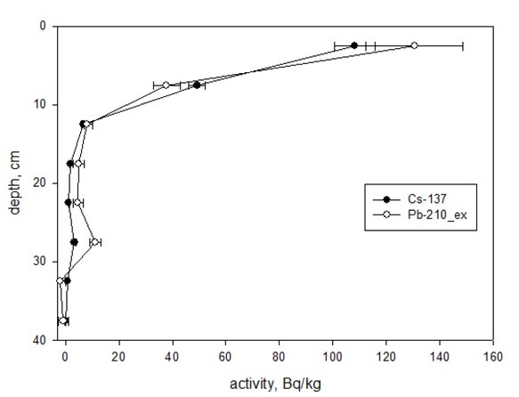
The 137Cs and 210Pbex inventories measured for the soil cores from the agricultural field range from 730 to 7911 Bq·m–2 and from 1615 to 11136 Bq·m–2, respectively (Figs. 2–3). To calculate the rate of soil erosion and sediment accumulation, the reference inventories of 137Cs and 210Pbex need to be known. The reference inventories for 137Cs and 210Pbex were measured in undisturbed soil cores collected from the area surrounding the study field. Fig. 7 provides an example of the depth distributions of 137Cs and 210Pbex at the reference site. 137Cs was found at a depth of about 25–30 cm and, simultaneously, 210Pbex was found at a similar depth. Both depth distributions show an exponential decrease with depth, however, the maximum 137Cs concentration was just below the surface. This behaviour of caesium in soil has also been described by Li et al (2009). Based on the reference cores, the reference inventories were estimated. The mean value of the total baseline inventory of 137Cs for the study area is 2627 Bq·m–2. This value is substantially higher than the mean value for Poland (Pietrzak-Flis, 2000; Strzelecki et al, 1994). This is because the study area is located in the region where larger 137Cs concentrations in soil are expected due to the Chernobyl accident. The values of Chernobyl 137Cs depend on the trajectories of the main radioactivity clouds, and on the precipitation in the area of interest at the time of the accident (Stach, 1996; Strzelecki et al, 1994). Increased values of Chernobyl 137Cs concentration are found along the line of Warsaw – Opole – the Kłodzko Basin. The largest values of Chernobyl 137Cs fallout were found in the Opole and Silesia regions (SW Poland), and in the Kłodzko Basin in the foreland of the Sudetes Mountains. In these areas, the values of Chernobyl 137Cs concentration were between 15.6 kBq·m–2 and 19.3 kBq·m–2, with the maximum value of 96 kBq·m–2 in the Nysa area (Stach, 1996; Strzelecki et al, 1992, 1994; Szewczyk, 1994). The strong spatial variability of the 137Cs concentration from the Chernobyl accident makes it difficult to use 137Cs in soil erosion studies (Golosow et al, 1999). The mean value of the137Cs deposition for the Świętokrzyskie region is 1.28 kBq·m–2, and the range is from 0.31 to 3.55 kBq·m–2 (Issajenko et al, 2014). Unfortunately, the authors of that study collected only the top 10 cm of soil, thus this value could be systematically lower than in our case. The mean value of 137Cs deposition for Poland is 1.53 kBq·m–2, and the range is from 0.22 to 17.79 kBq·m–2 (Issajenko et al, 2014).
The calculated 137Cs reference inventory, based on latitude and mean annual precipitation for the study area, is 1269 Bq·m–2. To use a more sophisticated model to calculate soil erosion based on the 137Cs inventories, knowledge of the annual fallout of 137Cs is needed. Unfortunately, the approach described above does not provide this information. There are few places in the world where the deposition of 137Cs has been measured since nuclear weapon tests started, and the information about the rate of fallout is essential to use 137Cs to study soil erosion. In Poland, the deposition of 137Cs has been measured since 1970 (Stach, 1996). The concentration of Chernobyl 137Cs varies widely even within one field (Dubois and Bossew, 2003; Strzelecki et al, 1992, 1994; Szewczyk, 1994). The percentage of the Chernobyl deposition in the global deposition of 137Cs must be known to be able to use the models to calculate soil erosion from the 137Cs activity data. Nowadays, there is a problem with separating the Chernobyl fallout from global 137Cs fallout. A valuable tracer of the Chernobyl fallout was another caesium isotope 134Cs, but this isotope has a relatively short half-life (approx. 2 yr) and is no longer present in the environment. The annual fallout of 137Cs could be obtained according to calculations proposed by Walling and He (1999), but this approach seems to be an over-simplification due to changes in the 137Cs fallout in the past and local rainfall distribution. In the present study, the reference inventory of the 137Cs fallout was separated from the Chernobyl fallout and from the global weapon test fallout by estimating the baseline inventory from atmospheric records. Moreover, this method is useful to obtain information about the variability of the 137Cs deposition during the period of the fallout accumulation (Lu and Higgitt, 2000; Poręba and Bluszcz, 2007). This method allows us to estimate an initial inventory of 137Cs connected with nuclear weapon tests, based on the precipitation data (IMGW-PIB data - Institute of Meteorology and Water Management - National Research Institute) and data provided by Sarmiento and Gwinn (1986) (Poręba and Bluszcz, 2007). The global 137Cs fallout calculated by this model is 1456 Bq·m–2 (Fig. 8a). This value is connected with nuclear weapon tests and is also called the global caesium fallout. The difference between this value and the value of caesium fallout measured at the reference site is associated with the Chernobyl fallout. For the study area, about 45% of the total caesium fallout is connected with the Chernobyl accident.
Fig. 8
a) The calculated annual 137Cs inventories based on precipitation data and model Sarmiento-Gwinn for a study site; b) The calculated monthly 137Cs inventories based on precipitation data and model Sarmiento-Gwinn for a study site for the period 1962–1964
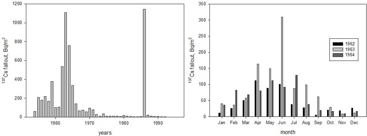
The 137Cs fallout calculations for the study area are presented in Fig. 8b. For the study area, about 44% of the global caesium fallout occurred in the period 1962–1964. These calculations take into account both the nature of rainfall and seasonal variations in rainfall over the period of fallout.
The mean value for the 210Pbex reference inventories is 4835 Bq·m–2. This value was obtained from the measurement of reference soil cores and is similar to values obtained by other authors (Porto et al, 2006; Kato et al, 2010). In this case, 210Pbex constant deposition flux was assumed and the annual fallout of 210Pb for the study area was estimated to be 150 Bq·m–2·a–1. Compared to 137Cs, which is frequently used to study soil erosion, 210Pbex is rarely used for this purpose. 210Pbex is mainly used to study the sedimentation rate of lake sediments or peat accumulation. Nowadays, knowledge concerning the global values of 210Pbex is also limited (Baskaran, 2011; Mabit et al, 2014) and the range of the 210Pbex fallout is relatively large.
Based on the reference values of 137Cs, about 62% of the study area was defined as eroding while, based on the 210Pbex inventories, this figure was about 50%. The simple comparison between the measured value of the 137Cs or 210Pbex inventories and the value of the reference inventory of 137Cs or 210Pbex allows us to recognize erosion and deposition areas; however, to obtain quantitative estimates of soil erosion, one of several available models must be used (Walling and Quine, 1990). To estimate soil erosion based on 137Cs and 210Pbex, the proportional model (137Cs) as well as mass balance models (137Cs, 210Pbex) were applied (Walling and Quine, 1990; Walling and He, 1999; Poręba, 2006). The results of calculations for soil erosion for the valley section in question, using the four models, are presented in Fig. 9. The calculated soil erosion for the studied area shows significant variation. In the case of the 137Cs measurement and the proportional model, the obtained soil loss results vary from 0.49 to 3.99 kg·m–2·a–1, whereas in the case of the simplified mass balance model the range is from 0.61 to 7.89 kg·m–2·a–1. The soil erosion rates calculated by the
Fig. 9
The spatial patterns soil erosion and sediment accumulation calculated by different models based on radionuclide inventories on the studied agricultural field: a) proportional model based on 137Cs inventories, b) simplified mass balance model based on 137Cs inventories, c) improved mass balance model based on 137Cs inventories, d) improved mass balance model based on 210Pbex inventories.
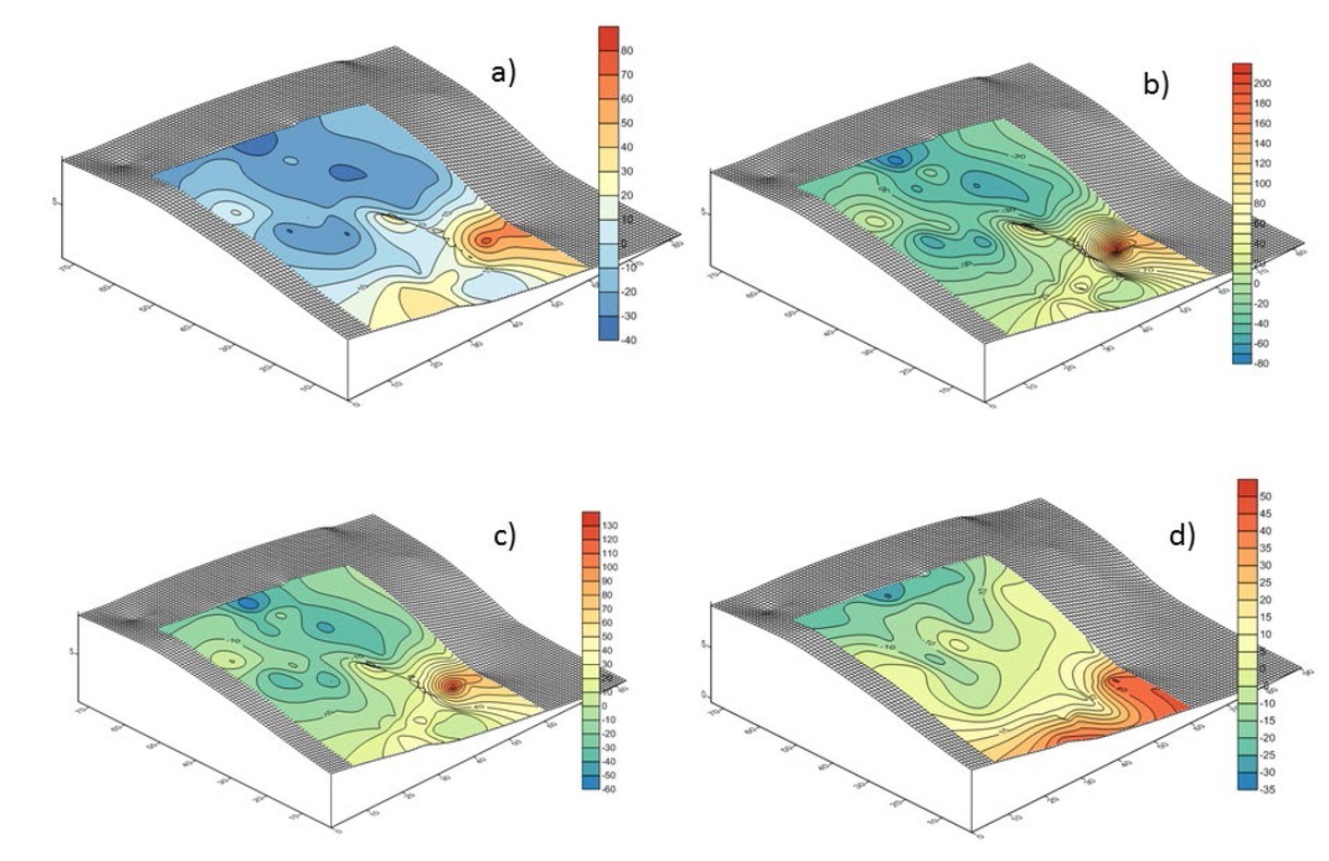
improved mass balance model for the cultivated slopes vary from 0.35 kg·m–2·a–1 to 5.98 kg·m–2·a–1. The mean soil erosion rate calculated for the proportional model is 2.09 kg·m–2·a–1, the mean soil erosion rate for the simplified mass balance model is 3.35 kg·m–2·a–1, with 2.18 kg·m–2·a–1 in the case of the improved mass balance model. The results obtained by the proportional model and improved mass balance model are similar, while the results of soil erosion loss obtained using the simplified mass balance model are substantially higher. The simplified mass balance model assumes that the entire caesium fallout occurred in one year, which might be a source of error in the case of areas contaminated by the Chernobyl caesium fallout. In the case of the improved mass balance model, the monthly (or at least annual) values of caesium fallout, as well as the initial distribution of fresh fallout of caesium in the top soil, are considered. Still, the improved mass balance model probably provides the most reliable results, but requires several additional parameters (Walling and He, 1999; Poręba and Bluszcz, 2008).
The soil erosion estimation based on the 210Pbex measurements and the improved mass balance model ranged from 0.22 kg·m–2·a–1 to 3.07 kg·m–2·a–1, with a mean value of 1.38 kg·m–2·a–1.The range of calculated soil erosion is similar to that obtained by the proportional model or improved mass balance model in the case of caesium measurement, but the mean value of soil erosion is slightly smaller than the values obtained in those latter cases. That difference can be attributed to different periods covered by measurements of caesium and lead. The results suggest an intensification of soil erosion after 1950. The change in land use is also supported by a different distribution of the intensity of the erosion and accumulation processes within the examined slope. In the case of 137Cs, large soil erosion values were obtained in the middle part, but in the upper part of the slope for 210Pbex. However, the accumulation in the case of the 210Pbex isotope analysis is greatest for the zone just above the edge of the gully (mean value 26 cm during 100 years) while the greatest accumulation for the 137Cs isotope measurement is approximately 10–15 m from the edge of the ravine (mean value 25 cm during 54 years). This may be the result of changes in land use after World War II. As a result of intensive mechanical cultivation, the slope has been remodelled.
It is quite clear that the soil erosion rate calculated on the basis of radioisotope data depends on the model used; still we can note that the proportional model and the improved mass balance model provide similar results. Similar discrepancies between the results obtained by different models are also present when calculating sediment accumulation. In this case, the results using the proportional model and the improved mass balance model are also similar, whereas those of sediment accumulation obtained using the simplified mass balance model are slightly higher. Surprisingly, sediment accumulation at the foot of the slope for two sampling points by 137Cs measurements was close to zero, which suggests no sediment delivery to those locations. This is also confirmed by the depth distribution of isotopes in the sediment profiles.
Results of OSL dating
OSL samples from four locations within the study area were analysed: one sampling location at the top of the slope, one located in the eroded part of the slope, one at the foot of t he slope and one from the wall of a gully located at the foot of the studied slope. The locations of sampling points for luminescence dating on the slope are marked in Fig. 3. Figs. 10–13 present the results of OSL dating for soil samples collected from the sampling positions on the slope (Figs. 10B–12B), a s well a s the samples collected from the gully wall (Fig. 13B). The results of OSL dating for the Biedrzykowice study site are also given in Table 1. This table also presents the results of radionuclide analysis in the dated samples, dose rate calculations and doses. To determine OSL ages, the central age model (CAM) proposed by Galbraith et al (1999) was used.
Fig. 10
The depth distribution of the 137Cs and 210Pbex (A), SAR OSL ages (B), grain size composition (C, D) and stratigraphy (E) for the soil core collected from the upper part of the slope.
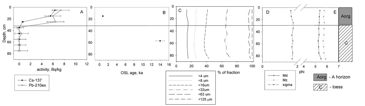
Fig. 11
The depth distribution of the 137Cs and 210Pbex (A), SAR OSL ages (B), grain size composition (C, D) and stratigraphy (E) for the soil core collected from the middle part of the slope.
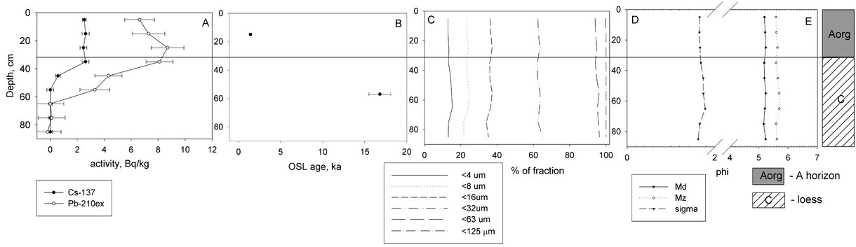
Fig. 12
The depth distribution of the 137Cs and 210Pbex (A), SAR OSL ages (B), grain size composition (C, D) and stratigraphy (E), for the soil core collected from the lower part of the slope.
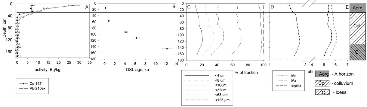
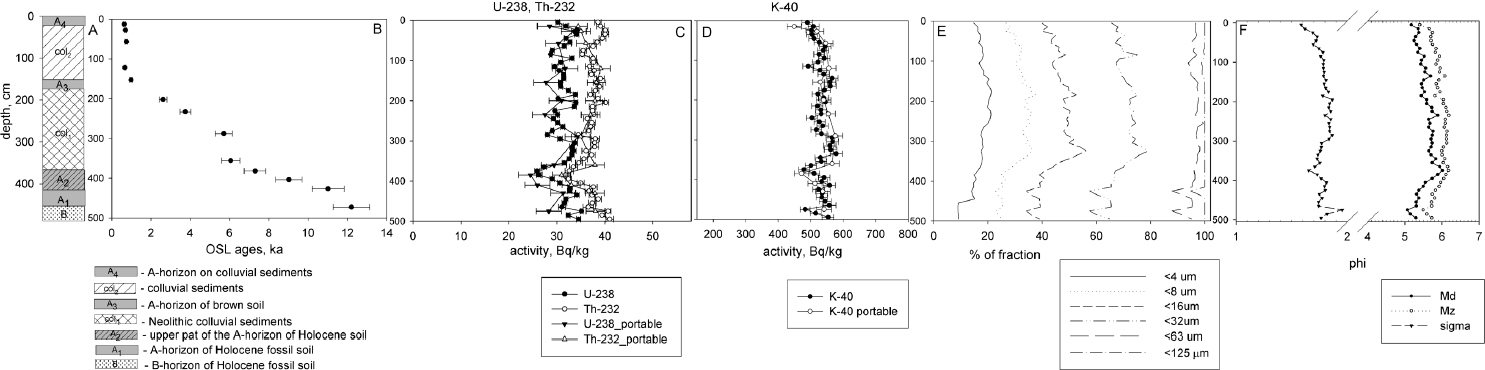
Fig. 13
The results of OSL SAR dating for the side of the gully (B), results of U-238, Th-232 (C) and K-40 (D) analysis as well as grain size analysis (E, F) in samples from the wall of gully. On the figure also shown the results of activity measurements by portable gamma spectrometer (B) and stratigraphy (A).
In the case of ploughed land, the luminescence ages of the deeper layer (loess) are between 14–17 ka (Bie_2_2 and Bie_3_2; GdTL-3068, GdTL-3070; Table 1). The OSL distributions are almost symmetric, thus the results from CAM model probably represent the true depositional age. The luminescence ages of the layers closer to the soil surface are between 0.779–1.42 ka (Bie_2_1 and Bie_3_1; GdTL-3067, GdTL-3069), and OSL age distributions are positively skewed and asymmetric. Those distributions could be a result of incomplete bleaching or post depositional processes, particularly as in this case we are dealing with both biological and mechanical mixing (in the form of the incorporation of
quartz grains into a ploughed A-horizon, Fig. 14) (Bateman et al, 2003). Due to pedoturbation (both biological and mechanical mixing) a part of quartz grains move up to the topographic surface where the luminescence signal may be bleached. Just before the sediment transport on the slope, or at the beginning of this process, more than 90% of the initial luminescence signal is bleached. Similar results have been obtained for sandy loess in the south of Poland (Poręba et al, 2015). In the case of sampling points located at the base of the slope, 5 sediment samples were OSL dated (Fig. 12). A ll OSL ages are consistent with a stratigraphic order. The age of the sediment sample from the top soil is equal to 0.175 ka (Bie_4_1; GdTL-3071). Below, very close to the surface, the age of the sediment sample equals 0.838 ka (Bie_4_2; GdTL-3072). The next part of the sediment core is represented by two luminescence results within the range 4.20–6.28 ka (Bie_4_3 and Bie_4_4; GdTL-3073, GdTL-3074). The younger results are probably due to bioturbation before covering by the next sedimentation. The result of OSL dating of the lowermost sample is equal to 12.28 ka (Bie_4_5; GdTL-3075). This is significantly younger than the expected age of loess cover formation, which may be the result of bioturbation before covering by Neolithic sediment.
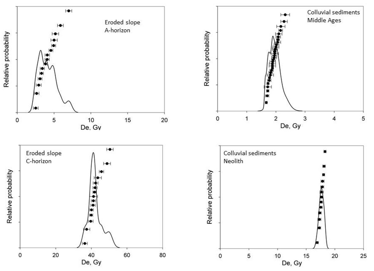
In the case of the gully wall sampling point, 13 sediment samples from different sediment horizons were collected for the luminescence study (Fig. 13). The age of the sediment sample from the top soil (modern humus soil-horizon) corresponds with the age of sediments collected on the eroded slope. The whole profile could be divided into three main parts. The upper part of the colluvial sediment is clearly the youngest part of the analysed profile, with four luminescence results within the range 0.645–0.746 ka (Bie_1_1 - Bie_1_4; GdTL-2906, GdTL-2907, GdTL-2908 GdTL-2909; Table 1). It can also be seen that all 4 dates are within a very small range. For the OSL samples of the middle part of the sediment profile, the results are within the range of 6.05–0.988 ka (Bie_1_5 – Bie_1_9; GdTl-2910, GdTL2911, GdTL2912, GdTL2913). The lowest dated samples of this part of sediment are connected with the beginning of Neolithic colluvium accumulation (6.05–5.71 ka). The sediment samples B_1_5-B_1_7 are visibly younger than the expected age. This could be a result of the post-sedimentation pedoturbation processes. The visible fossil soil at the ceiling of the top of this sediment profile could confirm this hypothesis. The results of OLS dating for the lowest part of this sediment profile are within the range from 12.22 ka to 7.30 ka (Bie_1_9 - Bie_1_13; GdTL-2914, GdTL-2915, GdTL-2916, GdTL-2917). Those samples were taken from the Late Pleistocene-early Holocene fossil soil. The lowest sample is from the B horizon of fossil soil, whereas the rest of the sample comes from the A horizon of fossil soil. The results of OSL dating for the humus horizon are visibly younger due to the rejuvenation by pedoturbation during the Holocene. The results of OSL ages for the lower part of the A horizon of the Late Pleistocene – Holocene fossil soil are comparable with the previous results of 14C dating (Śnieszko, 1995).
Results of grain size analysis
The results of particle-size analysis, along with the depth distributions of 137Cs and 210Pbex and OSL ages for three locations on the slope (top, eroded part and foot of the slope) are presented in Figs. 10–13. The studied sediment is characterized by only slight variations in grain-size distributions in the zones where the studied radionuclides (137Cs and 210Pbex) occur. Two profiles presented in Figs. 10C and 11C have similar grain-size distributions. Silt is the dominant fraction varying between 77 and 80% and fine silt is the larger subfraction and increases relatively to coarse silt at the base of the solum.
The clay content (<4 μm) is constant and fluctuates between 13.0 and 15.5%. Sand (>63 μm) content also varies little and is less than 10% of the total sediment. The sediments are very poorly sorted (1.56–1.8 ϕ) and the mean grain size (Mz) varies little (5.04–5.6 ϕ). The profile presented in Fig. 12C shows an increasing clay fraction with depth through the colluvial sediment. Below the colluvial layer, Mz decreases slightly (Fig. 12D).
The sequence presented in Fig. 13E has a particle-size distribution which reflects the lithogenic and pedogenic character of particular layers. Shifts between neighbouring units are visible, as is the base of the solum. Clay content is very high (9.5–21.3%) in the middle layer (older colluvium) and lo wer in the lower part of the oldest soil. Maximum clay content is in the Bt horizon of the lower unit, and the minimum is in the uppermost A horizon (10%) and the lower part of the lower colluvial layer. The biggest fluctuations in particle size distribution are recorded in clay and sand content (9.5–21.3% and 0.5–12.0%, respectively). The whole sequence is poorly sorted (δ = 1.6–1.9 ϕ), mean grain size (Mz) varies between 5.0 and 6.0 φ (15–29 μm) and average grain size is 21 μm (Fig. 13F).
Micromorphology
Typical micromorphological features (Table 2, Fig. 5) of the lowest soil unit (depth 380–475 cm) are: channel microstructure (common in the whole sequence), clay microfeatures and Fe-Mn nodules (especially common in the middle part). Additionally, the upper part is rich in faecal pellets and pieces of charcoal. Microscopic observations of thin sections showed a “typical” record of occurrence of pedogenic microforms. The clay coatings, infilling recorded inside the channels and fissures are the effect of illuviation processes and the formation of well-developed Bt-argic horizons. The other microfeatures mentioned are also typical pedogenic features, confirming a high level of soil development – Fe-Mn nodules are redoximorphic features; while charcoal pieces – pedogenic ones. According to palaepedological criteria for the area of the Southern Polish Loess Upland, this type of palaeosol can be described as a buried mature soil developed at the end of the Late Glacial and Early Holocene (e.g. Jersak et al, 1992; Konecka-Betley, 2002).
Table 2
Micromorphology of colluvial-soil sequence at Biedrzykowice. Microstructure: ch – channel, co – coprolithic, ma – massive. Frequency of occurrence: 0 – none, 1 – single, 2 – few, 3 – common, 4 – very common.
The middle unit (151–360 cm; Table 2; Fig. 4) has very similar micromorphological characteristics, but the distribution of diagnostic features is very specific. In the thin sections, all the features mentioned above were also identified. The Fe-Mn microfeatures and fecal pellets were recorded in the whole unit as common and very common forms. The unit is clear ly two-parted, with a division according to the presence of charcoal and clay microfeatures. The upper part is rich in illuvial microforms and also in – but less common – charcoal. Angular clay concentrations are very specific – their distribution is not associated with commonly present biogenic channels. Chaotically arranged clay particles are frequently present inside the groundmass. The micromorphological characteristics suggest this unit is a colluvial soil developed on older, redeposited soil material. The presence of clay features testifies to the parent material of this soil coming from a redeposited Bt soil horizon.
The main microfeatures of the upper unit (0–124 cm; Table 2) correspond with those of the middle unit, but their degree of development is much weaker. The top horizon clearly has pedogenic features – modern faecal pellets and charcoals are common. There are no traces of illuviation and redoximorphic features. The middle and especially lower units have clay and Fe-Mn features (single to common) and faecal pellets (common). The unique features are clay coatings – thin and continuous on the walls of channels. This set of micromorphological features testifies to young pedogenic processes. The lack of older, redeposited clay microforms indicates that the parent material was not directly connected with the older and well developed Bt soil horizon. According to our results of micromorphology analysis, it cannot be excluded that the redeposited material of upper soil horizons of Holocene soil was the parent material of the young soil.
Dendrochronology
Below, the results of dendrochronological analyses are presented for samples taken from trees growing at the base of the slope near the edge of the gully.
Tree no. 1
The tree is tilted perpendicularly to the gully axis, about 75% of its root system is exposed. The distance between the furthest exposed root and the hillslope edge is 1 .5 m. The tree we sampled has grown since at least 1938. It was not possible to determine eccentricity because it was not possible to sample a core from the side of the tree exposed to the gully. Strong ring reductions were found in 1970–1978, 1986–1989, 2010–2013 (Fig. 15A).
Tree no. 2
The tree is tilted perpendicularly to the gully axis, about 25% of its root system is exposed. The distance between the furthest exposed root and the hillslope edge is 0.5 m. The tree we sampled has grown since at least 1960. Eccentric growth of the tree started in the following years: 1977, 1981, 1996, 1999, 2000, and 2014. Strong ring reductions were found in 1970–1978, 1986–1989, 2010–2013.
Tree no. 3
The tree is tilted perpendicularly to the gully axis, about 50% of its root system is exposed. The distance between the furthest exposed root and the hillslope edge is 0.9 m. The tree we sampled has grown since at least 1949. Eccentric growth of the tree started in the following years: 1978, 1979, 1983, 1984, 1996, 1998, 1999, 2002, 2010, 1015, 2016. Strong ring reductions were found in 1961–1963, 1968–1973, 1989–1994, 2005–2011 (Figs. 15B, 15C).>
Tree no. 4
The tree is tilted perpendicularly to the gully axis, about 50% of its root system is exposed. The distance between the furthest exposed root and the hillslope edge is 0.6 m. The tree we sampled has grown since at least 1953. Eccentric growth of the tree started in the following years: 1957, 1963, 1975, 1976, 1981, 1987, 1996, 2008, 2014, 2016. Strong ring reductions were found in 1970– 1976, 1968–1973, 1998–2002, 2010–2017.
Tree no. 5
The tree is tilted perpendicularly to the gully axis, no roots were exposed, tree growing at the distance of 1 m to the gully hillslope edge. The tree we sampled has grown since at least 1949. Eccentric growth of the tree started in the following years: 1957, 1963, 1975, 1976, 1981, 1987, 1996, 2008, 2014, 2016. No strong reductions were found.
Tree no. 6
The tree is tilted perpendicularly to the gully axis, about 50% of its root system is exposed. The distance between the furthest exposed root and the hillslope edge is 1 m. The tree we sampled has grown since at least 1948. Eccentric growth of the tree started in the following years: 1961, 1963, 1971, 1973, 1978, 1980, 1986, 1988, 1993, 1996, 1999, 2002, 2014, 2016. Strong ring reductions were found in 1983–1998, 2010–2015. Additionally from this site, the exposed roots of the studied tree were collected. Roots were exposed: no. 1 – 1993, no. 2 – 1998, no. 3 – 2008, no. 4 – 2014.
. Discussion
The calculated sedimentation rate for modern soil erosion, based on the 137Cs and 210Pbex measurements, ranges from almost 0 to 4.5 mm·a–1. The calculated total thickness of soil eroded obtained by the 137Cs and 210Pbex measurements is quite similar and ranges from 0 .3 to 23 cm and from 0.1 to 22 cm, respectively. In the case of sediment accumulation, the calculated total thickness of the accumulated sediments ranges from 4 to 46 cm in the case of the 137Cs measurement and from 1 to 33 cm in the 210Pbex measurements. The apparent similarity of the results obtained with both isotopes is somewhat surprising, taking into account the range in time of both methods. One possible explanation is the possible change in land use that took place after World War II. There are also visible differences in distribution on the surface of the field between the results of soil erosion and sediment accumulation obtained using the 137Cs and 210Pbex methods. The 210Pbex method indicates that the upper parts of the slope are eroded and a more gradual increase in accumulation takes place from more or less half of its length. In the case of 137Cs, the spatial distribution of erosion and accumulation intensity is slightly different. Rather, it remodels the surface of the slope, and the largest accumulation takes place higher than in the 210Pbex analyses. The eroded material probably does not reach the edge of the gully (former valley bottom) from the change in land use. Additionally, for the upper part of the colluvial sediment samples collected from the wall of the gully, a limited sediment accumulation was observed for the last 50–100 years. Both the isotope depth distributions, as well as the values of isotope inventories, confirmed this hypothesis. For those sampling points, 137Cs as well as 210Pbex are present only at the top of the modern A-horizon, which confirms that no mechanical mixing has occurred in this location over the last 50–100 years. The depth distribution of both isotopes, together with the inventories of 137Cs and 210Pbex , suggest that limited sediment delivery during the last 100 years occurred to the site at the edge of the gully. This delivery was probably before the fallout of 137Cs which occurred after the Chernobyl accident. Samples B_1_1 to B_1_4 (gully wall) were dated by the OSL method as medieval colluvial sediment (Table 1). At the depth from 150 cm to 365 cm, there is a layer of Neolithic colluvial sediment with visible pedologic features, which was already present by the end of sediment accumulation. Below the Neolithic colluvial sediment are the A and Bt horizons of the Late Vistulian-Early Holocene fossil soil. The OSL dating results of this fossil soil are smaller than the time of its formation. This is due to the rejuvenation of this upper layer of fossil soil before its covering by Neolithic settlements. The situation is similar in the case of Neolithic colluvia, where the upper layer is also rejuvenated. The bleaching process of the OSL signal probably occurred from the end of Neolithic sedimentation to the cover of medieval settlements. The obtained results of micromorphological analyses also seem to confirm this conclusion
For the sediment core located at the foot of the slope, the OSL age of the sediment is 0.175 ka. Although this layer contains 137Cs activity, its depth distribution and inventory suggest no sediment delivery for at least 60 years. The 137Cs and 210Pbex inventories also confirm the lack of modern sediment. Thus, this OSL age result seems to be reliable. For samples from the deeper layers, the OSL ages correspond to the ages of samples collected from the gully wall. Gully erosion and surface erosion after the deforestation of dry valleys took place simultaneously. The formation of a gully means that agrotechnical treatments on the slopes of the dry valley in which the gully has formed no longer reach its edge. If the area of a gully and its periphery is re-forested, the flow of material eroded away from the farmed slope of the dry valley to the edge of the gully ceases. Hence, in the Holocene water erosion soil profile that was exposed in the gully wall, no record of sediment caused by erosion of the dry valley slope used for agriculture has been found since the time of afforestation of the gully began.
The medieval colluvial sediment is about 150 cm thick, while the thickness of the Neolithic colluvial sediment is about 180 cm. Unfortunately, there are difficulties in precisely establishing the age of the latest Neolithic colluvial sediment due to pedoturbation. In the case of medieval sediments, the upper layer might have been rejuvenated as well, however, it is significantly less pronounced than in the case of the Neolithic colluvial sediment. While 50 cm of sediment has accumulated over the last 50 years, only about 180 cm of sediment accumulated during the few hundred years of the Neolithic. Thus, in the case of medieval sediment, it can be concluded that the layer of about 150cm thickness accumulated in a very short time. The relatively small age range of medieval sediment suggests that the intensity of erosion at that time exceeded even what we are seeing nowadays. Similar results indicating an increase in medieval erosion have been noted by Fuchs et al (2011). Most probably, the present gully developed quite rapidly as a result of increased runoff and developing furrow erosion. It is worth noting that the Biedrzykowice settlement was probably founded in the 14th century. The first mention was around 1389 A.D.; however, farmed terrain could have started earlier. The first menti on of Działoszyce (4 km from Biedrzykowice) is about 950 A.D. (Schmidt and Heinrich, 2011). It seems, however, that the start of re-using the area was not the reason for such intense erosion. It could have been connected with increased rainfall in the fourteenth century. The catastrophic rainfall in this period and increased erosion in Europe were mentioned by Dotterweich and Dreibrodt (2011). Dotterweich (2003) concluded that the intensity of rainfall in the 14th century was unusually large, which in combination with the change in land use could be the reason for the great intensification of erosion processes in the 14th century.
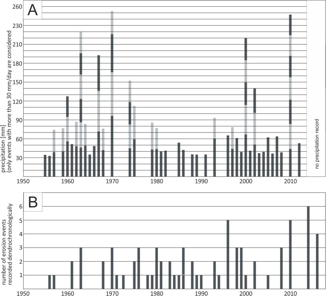
This resulted in the abandonment of this area as farmland, an invasion by woody vegetation, and consequently in the stoppage/minimization of erosion on the slope. Erosion processes re-started about 50–60 years ago, as indicated by the 137Cs and 210Pbex isotope measurements, probably due to land use change. The oldest sampled tree, one of the biggest in the studied gully started growing in the 1930’s. This indicates the period when in the gully began to grow trees. Fig. 16 presents the results of dendrochronological dating. We found over a dozen episodes when the hillslope of the gully retreated in the last 50 years, which indicates significant recent changes in gully morphology. Some of the events dated dendrochronologically correspond with large or numerous rainfall events recorded during individual years in the Sielec precipitation gauge located 12 km from the sampling site (1961, 1963, 1970, 1980, 1986, 1996, 1998, 2001, 2010). Dendrochronological data show more erosion episodes recorded in the last 20 years, but it doesn’t mean that erosion has intensified recently. It is more likely that trees have been closer and closer to the hillslope wall, and are more sensitive (their stems could be easily tilted when the root systems were exposed) to the following erosion events.
Fig. 16
Erosion events dated dendrochronologically (B) compared with rainfalls events recorded in Sielec gauge, dark and light grey colour were used one after the other to make more visible the individual rainfall events on the graph (A).
Long-term research on the Neolithic settlement in Bronocice, and its immediate surroundings in the vicinity of the specific site investigated by the authors, commenced in 1981. Studies on Holocene sediments in river valleys and dry valleys started shortly thereafter and the joint results of archaeological and geological research were published in 1996 (Kruk et al, 1996). At the time, the authors came to the conclusion that there had been an intensification of slope processes in the 5–4 ka BP period on the basis of many indirect premises. There was no direct evidence that could be provided by, for example, radioisotopic dating of slope sediments corresponding to periods of increased anthropogenic soil erosion. The results obtained now by the authors of the present paper finally prove, fully and reliably, the previously formulated theses and allow any prior reservations raised due to the uncertainty of relative dating to be rejected.
The intensification of agricultural colonization in the studied area in the Middle Ages, now confirmed in radiometric dating, has been documented historically as well (Śnieszko, 1985). As in the case of research on the Neolithic colluvium, prior to these measurements there was similarly no direct indisputable evidence of the presence of medieval colluvial sediments corresponding to agricultural land use.
Radiometric measurements of the sediments in Biedrzykowice also confirm another well-established hypothesis in the studies of local pre-history: that of significantly decreased agricultural pressure in the Bronze Age and in the period of Roman influence, as settlements were dispersed and agriculture poorly advanced during that time.
. Conclusions
Colluvial sediment dating and erosion rate calculations based on radionuclide analysis were used to perform a detailed study of the Holocene sediment budget of a slope in a loess area in Poland. As shown by the analysis, the area has been contaminated by Chernobyl 137Cs fallout – although this contamination is not strong, the SMBM model is not reliable in this case. The IMBM model, although more complicated, seems a much better choice for the study area. Similar results were obtained using the proportional model. The results of soil erosion obtained with the 210Pb isotope measurement method are smaller and have different spatial variability. This probably reflects the changing agricultural use after World War II.
Modern soil erosion based on results from the 137Cs method is 2.1 kg·m–2·a–1, whereas that obtained by the 210Pbex method equals 1.4 kg·m–2·a–1. The rate of erosion on the slope is quite variable. About 100% of the eroded soil has accumulated at the base of the slope. The mean thickness of modern sediment is 30 cm, the thickness of medieval sediment is about 155 cm, with Neolithic sediment about 180 cm thick. Sedimentation rates for the Neolithic sequences compared to those of the medieval periods are lower. The results suggest that the increased intensity of water soil erosion on the sl opes was one of the results of human impact on the environment. The start of sediment accumulation is correlated with the beginning of Neolithic farming. Although the thickness of medieval sediment is less than that of Neolithic sediment, the intensity of soil erosion was probably highest shortly after the reintroduction of farming in the Middle Ages, when gully formation had already started. The current intensity of soil erosion is probably lower than in the past and equals a few cm (up to 23 cm) for the last 50 years. The pattern of soil erosion on the slope suggests that we are currently witnessing slope sediment water transport with redeposition still on the slope.
The precise dating of colluvial sediment suggests that the sedimentation rate and thus also the erosion intensity for the Middle Ages was probably higher than nowadays. The OSL dating results show that colluvial sediments could indeed be dated by this method with sufficient precision, despite the rather short transport of quartz grains on the slope - mainly because the bleaching of the OSL signal begins even before the transport of grains on the slope, and finishes after burial by the next sediment layer at the accumulation site. Simultaneous use of the OSL dating method, the 137Cs and 210Pbex isotopic methods and of detailed pedological analysis allowed us to establish a reliable sediment chronology and reconstruct the history of soil erosion and sediment accumulation.
Gully erosion and surface erosion after the deforestation of dry valleys take place simultaneously. The formation of a gully means that agrotechnical treatments on the slopes of the dry valley in which the gorge has formed no longer reach its edge. If the area of a gully and its periphery is re-forested, the flow of material eroded away from the farmed slope of the dry valley to the edge of the gully ceases. Hence, in the Holocene water erosion soil profile that was exposed in the gully wall, no record of sediment caused by erosion of the dry valley slope used for agriculture has been found since afforestation of the gully began.