
. Introduction
Research conducted in various parts of the world indicates a rise in the activity of mass movements, including an increase in the number of landslides, in recent decades (Innes, 1983; Winchester and Chaujar, 2002; Petley et al., 2007). The reason for this increase is greater precipitation, e.g. in the case of Asia. Attention is also paid to the growing population and increasing development of areas threatened by the occurrence of landslides (Guzzetti et al., 2009; Petley, 2010; Malik et al., 2017). The rising frequency of landslides has resulted in an increasing number of buildings and elements of infrastructure’s being destroyed, and a growing number of people killed. For example, on 23 July 2002, in Kathmandu, very heavy rainfall caused a landslide of 9,000 m3, which turned into debris flow and floods, causing 16 human deaths (Paudel et al., 2003). Damages resulting from the landslide disaster and floods which occurred in Bosnia and Herzegovina in 2014 were valued at EUR 2 billion (15% of the country’s GDP); (Sandić et al., 2017).
In Duexi (China’s Sichuan province) a landslide with a volume of 8 million m3 was triggered, as a result of which 62 buildings and 1600 metres of road were destroyed, and 10 people were killed (Qui et al., 2017).
The increasing number of landslides and related economic losses have resulted in the development of new methods of mapping landslide activity, e.g. aerial and satellite imagery (Murillo-García et al., 2015; Schlögel et al., 2015), LIDAR data (Van Den Eeckhaut et al., 2007; Haneberg et al., 2009), and data from radar interferometry (Schlögel et al., 2015; Journault et al., 2018). The use of landslide maps can limit the destruction of buildings and infrastructure, and the maps developed by means of the above-listed methods are used for rational-spatial planning (Ives and Bovis, 1978; Bejar-Pizarro et al., 2017; Crawford et al., 2018). Special landslide monitoring techniques are used for particularly endangered areas, e.g. repeatable geodetic measurements, inclinometers or electrical resistivity tomography (Piegari et al., 2009; Lebourg et al., 2014; Bovenga et al., 2017).
Dendrochronology has also been used for developing maps of landslide activity (Catani et al., 2005; Lopez Saez et al., 2012). Until now, this method has not only been applied in geomorphology for landslide studies (Stefanini, 2004; Zielonka and Dubaj, 2009; Šilhán, 2017), but also for mapping the frequency of rockfall and debris flow events (Gärtner et al., 2003; Perret et al., 2006; Bollschweiler et al., 2007; Malik and Owczarek, 2009).
Dendrochronological techniques for landslide dating, which are used for the mapping of landslide activity and hazards, are based on the fact that the stems of trees growing on slopes are tilted during landslide episodes, which is reflected in the structure of their wood. Following tilting (after the landslide event), “reaction wood” is formed inside stems and tree rings start to become eccentric. These features of the wood anatomical structures, along with the macroscopic characteristics of the ring structure, allow landslide events to be dated with annual frequency (Demoulin and Chung, 2007; Gärtner and Heinrich, 2013; Lopez Saez et al., 2012). The analysis of both the wood anatomical structures and the macroscopic characteristics of the ring structure of tilted trees allows the dating of even small, unnoticeable, landslide events occurring over recent decades. However, there are only a few examples of the use of dendrochronology to develop maps of landslide activity, and they only relate to individual landslides (e.g. Catani et al., 2005; Stoffel, 2005; Lopez Saez et al., 2012; Malik et al., 2016; Šilhán, 2016). Authors have used various techniques for landslide mapping, e.g. GIS (Catani et al., 2005). Šilhán (2016) adopted a classical subjective method based on the analysis of “reaction wood”, along with a numerical method based on eccentric-growth analysis, to map landslide activity. The author took into account the changes in the sensitivity of trees to landsliding, related to the age of particular specimens. The research conducted so far has been limited to single landslide slopes, within which landslide activity maps and hazard maps have been developed, often by interpolating data from individual sites. To the best of the authors’ knowledge, dendrochronology has not been used for preparing a landslide hazard map on larger areas where there are both landslides with typical relief and areas without landslide relief. There are no examples of landslide hazard maps created on the basis of dendrochronological results for the entire mountain ridges or massifs. Therefore, the aim of the study was to develop a landslide hazard map for the massif of Sucha Mt (Beskid Żywiecki Mts, Western Carpathians, southern Poland), and also to propose a method which combines dendrochronological and geoinformatic tools to assess the spatial variability of landslide hazards over larger areas, greater than a single landslide slope.
. The study area
The study area is located on the massif of Sucha Mt (max 1040 m a.s.l.), in the Beskid Żywiecki Mts, in the Western Carpathians (Central Europe) (Fig. 1). The bedrock is composed of the sandstones and shales of the Magura Nappe (Stupnicka, 2013). There have been landslides of various types in the study area (e.g. flow-type, extensive rotational landslides, shallow landslides), mainly triggered by precipitation (Chen and Petley, 2005; Antronico et al., 2013; Netto et al., 2013; Pham et al., 2018).
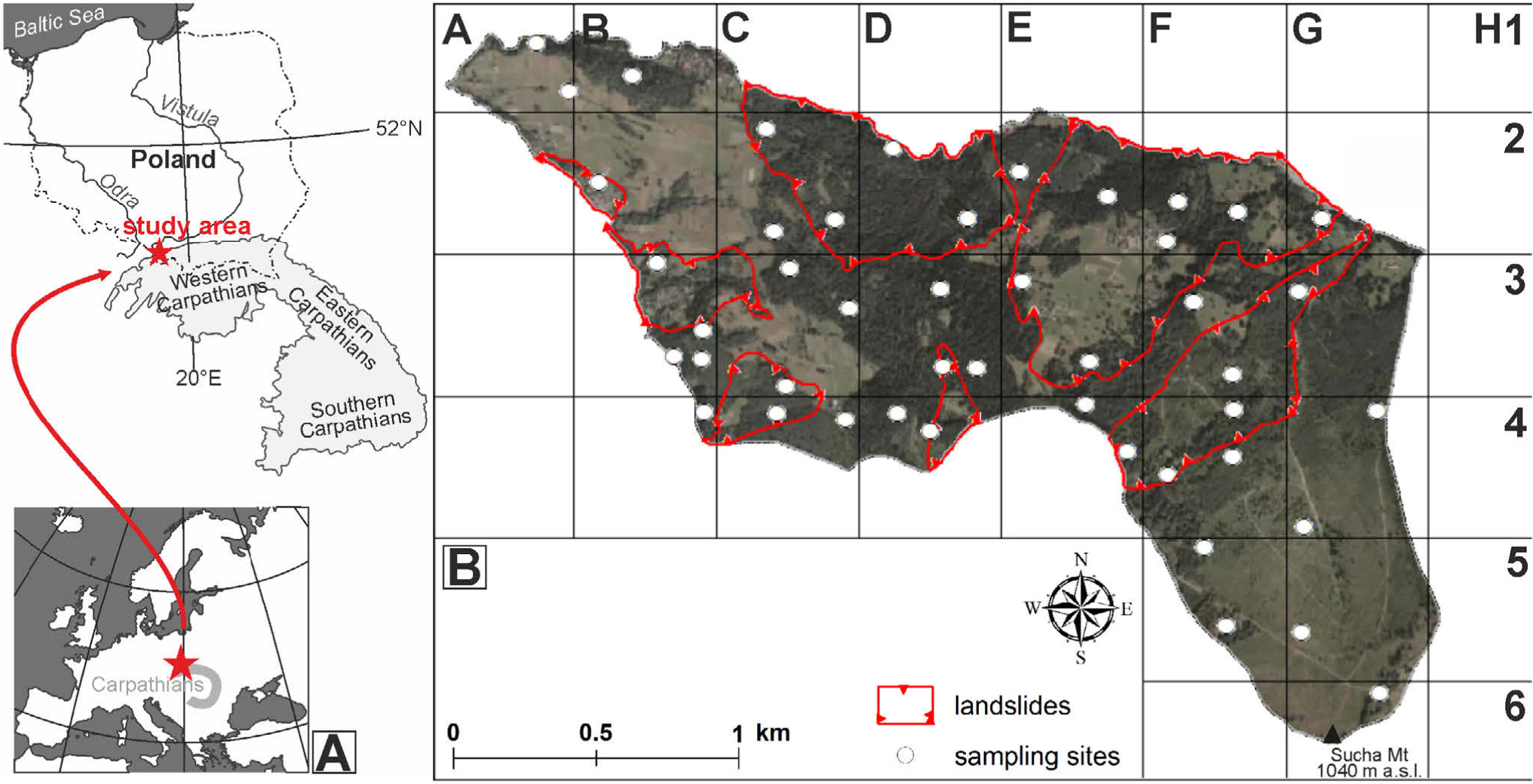
Fig. 1
The location of the study area in Central Europe, Western Carpathians (A) and the location of sampling sites for a dendrochronological study in the massif of Sucha Mt, in the Beskid Żywiecki Mts (B).
According to Hess (1965), the study area is situated in cold climatic zone with a precipitation of 1150–1350 mm. The average annual precipitation at the nearby gauging station (Żabnica, 550 m a.s.l.) is 1136 mm. The study area belongs to the lower montane vegetation belt, where common beech (Fagus sylvatica) and silver fir (Abies alba) are mainly expected to occur (Seneta and Dolatowski, 2008). Nowadays, as a result of forest management, natural forest communities have been replaced by planted Norway spruce (Picea abies).
Landslides occurring in the study area pose a threat to both people and infrastructure. In 2010, landslides were triggered in the study area and on the massif of Prusów Mt in Milówka, in the neighbourhood of the study area. The most hazardous landslide destroyed local road and electricity networks and 9 buildings, and blocked a stream valley, causing flooding.
. Study methods
Dating landslide activity from tree rings
Samples for a dendrochronological study were taken from Norway spruce trees (Picea abies) growing on the massif of Sucha Mt (3.75 km2). To ensure that the distribution of sampling sites within the study area was as even as possible, the study area was divided into 26 squares, each with sides of 500 m. A total of 46 sampling sites were selected from the 26 squares (Fig. 1B). The distribution of sites was determined by way of analysing the orthophotomap, illustrating the extent of coniferous forest, and excluding deforested areas or areas with deciduous trees from the study. The selection of the sites depended on the range of landslide slopes and stable slopes, and was determined based on an analysis of terrain topography from the Digital Elevation Model (DEM) (ESRI ASCII Grid, 2014). The DEM was prepared using the airborne laser-scanning data (LiDAR) with 1 × 1 m horizontal resolution and a vertical accuracy of 0.2 m (CODGiK, 2015). At least one sampling site was determined on each landslide slope and on each slope devoid of landslide relief.
At each site, samples (cores) were taken from the stems of 3 trees growing at a distance of several to several dozen metres apart. Samples were taken by means of a Pressler borer from trees whose stems had not been damaged and presented with no defoliation. Trees which were tilted transversely to the slope’s inclination were also excluded from the study. This is because most trees affected by landslide movements have stems tilted in axes parallel to the slope. Furthermore, all tilted spruces have deformed trunk cross-sections parallel to the direction of the tilting. For sampling purposes, we also selected trees whose circumference measured at chest height was at least 50 cm. Sometimes, it was not possible to find 3 spruce trees meeting the above-mentioned requirements at one sampling site, in the case of which cores were taken from 1 or 2 spruce trees. In total, samples were collected from 131 trees.
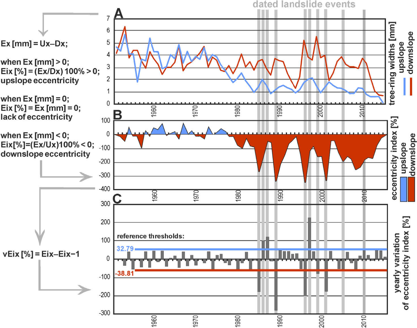
Two cores were collected from each tree: one from the upslope side of the tree and the other from the downslope side. The samples were taken at chest height, according to the slope’s inclination. The location of each tree was marked using GPS. The cores collected were glued into wooden holders and sanded, following which the tree-ring widths were measured with an accuracy of 0.01 mm (LinTab measurement station). The eccentricity, the eccentricity index and its yearly variation were calculated based on a comparison of the tree-ring widths found on the opposite sides of a single tree stem (method following Wistuba et al., 2013; Fig. 2). The dating of landslide events was made on the basis of the local reference threshold, obtained from trees growing on stable slopes (Wistuba and Malik, 2016). The thresholds represent an average level of yearly variation in the eccentricity index calculated from 10 spruce trees growing on a nearby slope devoid of any landslide relief. The upslope reference threshold is +32.79% and the downslope reference threshold is –38.81% (Fig. 2). The obtained results of the dendrochronological analyses provided the basis for determining the mean frequency of landslide events at each site, expressed as the average number of events occurring per decade. It was assumed that an event was indeed a landslide event when at least two of the trees sampled on a single site were disturbed by landsliding in one year. Sites where only one tree was sampled were omitted from further analysis.
Fig. 2
An example of dating landslide events from ring widths into (A) eccentricity, (B) eccentricity index [%] and (C) its yearly variation [%]:
U — tree-ring widths in the upslope part of the stem [mm];
D — tree-ring widths in the downslope part of the stem [mm];
E — the eccentricity of the tree-ring [mm];
Ei — the eccentricity index of the tree-ring [%];
vEi — the yearly variation in the eccentricity index [%];
x — year (annual tree ring).
Developing a landslide hazard map
The development of the landslide hazard map, based on the calculated average frequencies of landslide events at the sampling sites, made it necessary to select the adequate data interpolation method. ArcGIS software (ArcGIS Desktop, 2017) was used to determine the method of interpolation, and then the method of recalculation and visualisation of dendrochronological data.
The method of data interpolation for landslide activity in the study should be global. This means that it applies a single mathematical function to all measurement points (1); should be precise, i.e. all measurement data are located exactly on the surface to be interpolated (2); and should be deterministic – i.e. is used in a situation of sufficient knowledge about the surface being modelled, and allows the creation of the model as a clearly defined surface (3) (ArcGIS Help, 2017). We found that only 4 methods available in the ArcGIS software, i.e. Inverse Distance Weighted (IDW), Spline, Radial Basis Function (RBF) and Topo to Raster - met the above-listed requirements.
The IDW method was rejected at the beginning because it created structures of the “bull’s eye” type (unreal accumulations of counter lines around extreme values, thus generating unlikely surfaces). The remaining 3 methods of interpolation available in the ArcGIS software were analysed (RBF, Spline, and Topo to Raster). These methods best reflected the possible spatial distribution of landslide episodes identified on the basis of dendrochronological data (Fig. 3).
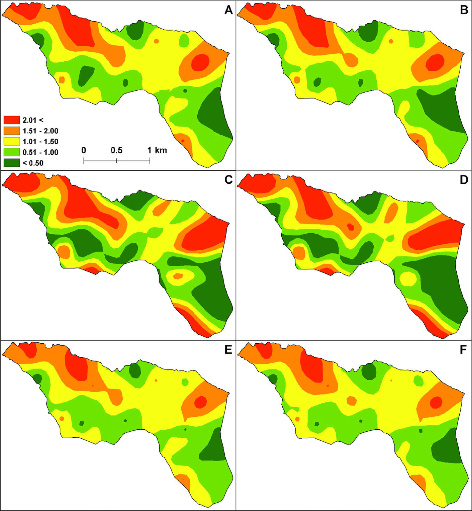
Fig. 3
The results of interpolation for all points (A, C, E), and without 5 control points (B, D, F). Interpolation methods: the Radial-Basis Function (A, B), Spline (C, D), and Topo to Raster (E, F).
The RBF method is conceptually similar to fitting a rubber membrane through the measured sample values (the surface passes through the data values) while minimising the total curvature of the surface. The basic function selected determines how the rubber membrane fits between the values (ArcGIS Help, 2017). The next method, Spline, estimates values using a mathematical function which minimises the overall surface curvature. This results in a smooth surface which passes exactly through the input points (Childs, 2004). The last tool, Topo to Raster, uses an interpolation method specifically designed to create a surface which more closely represents a natural drainage surface, and better preserves both ridgelines and stream networks. This technique creates hydrologically correct DEM’s, and is based on the ANUDEM program developed by Hutchinson (1989, 2011).
A visual assessment of the quality of the interpolation methods was made by comparing the results on the interpolation maps (Figs. 3A, 3C & 3E). An interpolation error was also determined for each method by removing 5 random-sampling sites and their values from the interpolation, and then comparing the differences in values before and after removing the points (Figs. 3B, 3D, 3F; Table 1). Table 1 shows the differences between the actual values of the 5 selected measurement points and the interpolated values. The errors reached values from – 0.91 (the Spline method) to +0.72 (the RBF method); on average they were –0.11. In addition, a Root Mean-Square Error (RMSE) tool was used to make use of the best method of interpolation. RMSE is the most frequently used parameter determining degree of accuracy. It expresses the dispersion of the distribution of the frequency of variances between the original (real) data and the interpolated data. In statistics and probability theory, RMSE is a widely used measure of conformity between a set of estimates and the actual values (Li, 1988). The calculated RMSE values were similar for the methods tested: from 0.49 (Topo to Raster) to 0.57 (Spline). Although the lowest RMSE value was obtained for the Topo to Raster method, the map using this method does not look realistic (Figs. 3E, 3F), as it contains errors relating to significant reductions in the range of values around individual points, not referring to the general trend of data variability in places with a weaker density of sampling sites. The RBF method presents a much better spatial distribution of landslide activity, but was rejected due to the lack of the possibility of imposing barriers, which are necessary for the correction of the automatic position of counter lines (ArcGIS Help, 2017). In the end, it was decided to use the Spline method, because the interpolation results obtained with this method do not have the limitations pointed out above.
Table 1
The calculated errors of the interpolation methods. A Root Mean Square Error (RMSE) expresses the differences between original (real) values (2nd column) and the interpolated values (3rd, 5th and 7th columns).
When presenting interpolated data we selected the intervals of the values of mean landslide activity per 10 years to be presented on the map of landslide activity: <0.50; 0.51–1.00; 1.01–1.50; 1.51–2.00; >2.00 (Fig. 5). The interpolation was carried out at a resolution of 10 × 10 m. During the interpolation, we used barriers – lines limiting the occurrence of landslide phenomena. Barriers were introduced into the map because in one sampling site we should divide two parts with different values of frequency of landsliding, e.g. when a watercourse or mountain ridge crossed a study area with one sampling site (Fig. 4; Fig. 6B). A layer of buildings and roads was superimposed on an interpolated map of landslide activity, and in this way the landslide hazard map was developed. The landslide hazards were shown on the map using 3 intervals: low (<1/10 years), medium (1–2/10 years) and high (>2/10 years); (Fig. 6B).
Fig. 4
The barriers applied in the process of dendrochronological-data interpolation in the massif of Sucha Mt, Western Carpathians, Poland: (A) watercourses, (B) the most-important ridgelines.
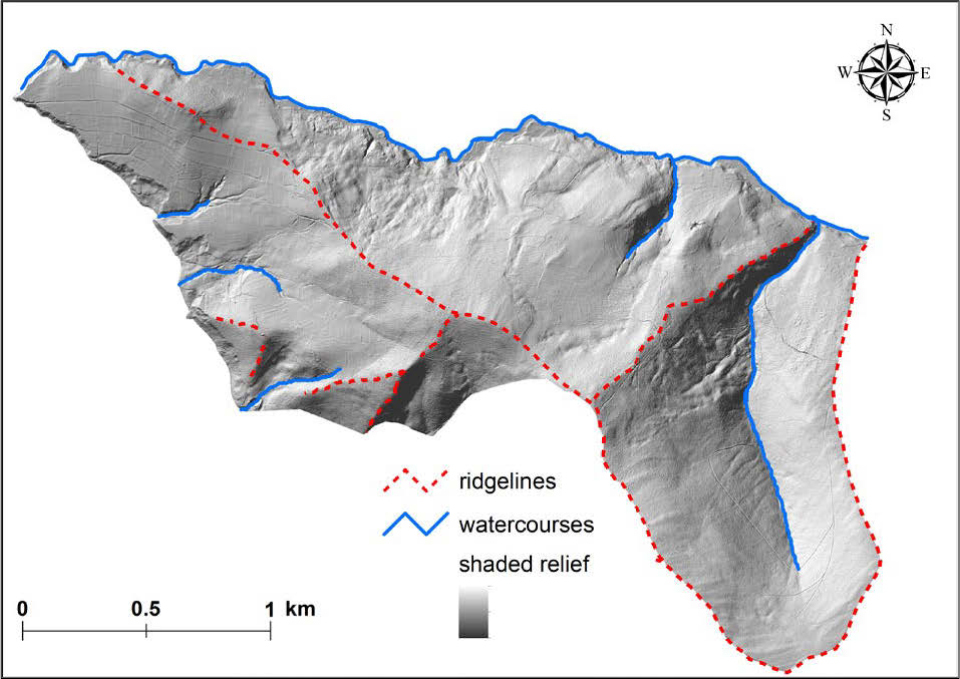
Fig. 5
Average frequency of landslide events calculated for each sampling site in the massif of Sucha Mt, Western Carpathians, Poland
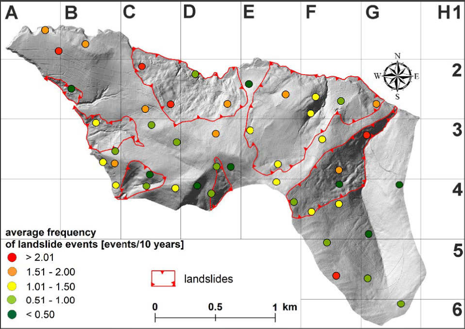
Fig. 6
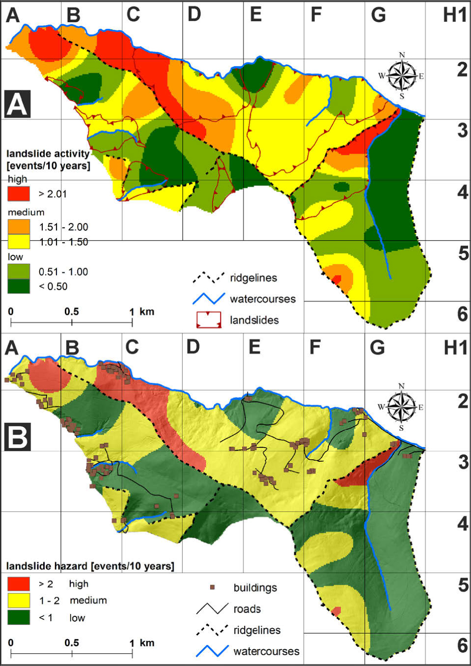
A landslide activity map developed on the basis of the selected interpolation method – Spline with barriers (A) and the landslide hazard map for the massif of Sucha Mt, Western Carpathians, Poland (B). Maps of the distribution of landslides were created on the basis of the results obtained from the tree-ring eccentricity analysis.
. Results
Tree-ring chronologies in the massif of Sucha Mt reach back to 1883. The sampled trees were from 15 to 133 years old, but only a few of them were very young (11.5% trees were less than 30 years old). Almost 51.9% of all trees were 50 or more years old, and 6.9% were more than 100 years old. A total of 282 landslide events were identified in 131 of the spruce trees which were sampled, and the earliest landslide event observed in the tree-ring series dated back to 1919.
The average frequency of landslide activity noted for each sampling site varies from 0 events/10 years (Fig. 5, square B2, E2) to 2.65 events/10 years (Fig. 5, square C2). Most of the sampling sites represent an average frequency of landslide activity from 0.51 to 1.0 events/10 years (12 sampling sites), and from 1.01 to 1.50 events/10 years (12 sampling sites). The highest frequency of landslide activity (an average of >2.0 events/10 years) was obtained for the southern part of the landslide, and near the headscarp of the largest landslide in the study area (based on the Digital Elevation Model) (Fig. 5, square C2; Fig. 6A). A high level of activity is also visible on the second largest landslide in the northern part of the landslide in the study area (Fig. 5, square G3; Fig. 6A), and on two slopes without landslide relief (Fig. 5, square A1, F5; Fig. 6A). Areas with a low frequency of landslide events are also visible on the map (Fig. 5, squares B2, C3, C4, D3, D4, F2, F4; Fig. 6A). Only 2 of the 46 sampling sites did not record any landslide activity (Fig. 5, square B2, E2; Fig. 6A).
The landslide activity map (Fig. 6A) shows that areas with high and medium activity often overlap with areas of landslides determined on the basis of the Digital Elevation Model from LiDAR data. However, some areas with particularly small landslides have low landslide activity (Fig. 6A, square B2, C3, D3, D4). There are also examples of areas with a lack of landslide relief, which show a medium or high frequency of landslide activity (Fig. 6A, square A1, B1, C4, D3, F5). Large landslides show internally variable levels of activity (Fig. 6A, square C2 and D2 or E2 and F2 or F3 and F4).
On the landslide hazard map, it was found that 84 buildings (65.62 %) and 5.28 km of roads (65.3 %) are located in the medium and high landslide-hazard zone in the study area (Fig. 6B). On the other hand, a relatively large number of buildings are located in low-hazard areas 44 (34.38 %). The areas where investments can be developed are also visible on the landslide hazard map. These are areas where the landslide hazard is low; they cover 38.2 % of the study area (Fig. 6B).
. Discussion
Dendrochronological data as a source for developing a landslide hazard map
Dendrochronological data provide data on the temporal and spatial variability of landslide activity in the past, with yearly (or even seasonal) resolution from recent decades up to hundreds of years (depending on stand age) (Shroder, 1980; Butler, 1987; Schweingruber, 1996). In this study, we used each tree growing on a landslide as a separate living sensor of ground movement, recorded as macroscopic characteristics of the ring structure, such as tree-ring eccentricity.
One of the problems encountered in developing landslide hazard maps, based on the use of the dendrochronology, is the selection of wood anatomical structures. Usually, two features of wood anatomy, i.e. growth eccentricity and “reaction wood”, are taken into account in the assessment of landslide activity (Stoffel et al., 2013; Corona et al., 2014). The eccentricity of tree growth is a measurable feature, while “reaction wood” is based on the subjective assessment of the researcher, and it sometimes proves very difficult to definitively allocate the wood being examined as “reaction wood” (Migoń et al., 2010). Therefore, dating the eccentric growth of trees seems to be a better method for developing a landslide activity map than the dating of “reaction wood”.
Another problem is the selection of trees from which samples (cores) will be taken for analysis. The first limitation refers to the distribution of trees. Usually, some areas mapped on the basis of interpolation are not forested, and of course, landslide activity cannot be determined for these areas. The species composition of the stand from which samples are taken is also important. The wood anatomical structures which develop in trees affected by landsliding have been best recognised in conifers, spruce in particular (Stoffel et al., 2013). When deciduous trees grow over the study area, it is more difficult to use dendrochronology to assess landslide hazard, mainly due to the limited focus on deciduous trees in former studies on landslide activity (Šilhán et al., 2014). The age of the stand in which the study is carried out can significantly affect the results. Ideally, if the trees are relatively old and similar in age, the results obtained can be easily compared with one another. However, in the case of very large areas covered by the study, it is extremely difficult to find trees which meet these requirements. Trees usually differ in age, and younger trees do not record older landslide events (Šilhán and Stoffel, 2015).
It is also indispensable to carefully select the sampling sites where the cores will be taken from trees. It is not enough to distribute the sampling sites at equal distances from one another. The distribution of the sampling sites should be dependent on the location of the landslide areas visible on the Digital Elevation Model developed from the LiDAR data (and, if possible, otherwise visible on topographic maps). Using the Digital Elevation Model, sampling sites should cover each separate slope and the surface of individual landslides visible on the map.
At the stage of editing the map, once the study of dendrochronological samples in the field and in the lab is completed, we should choose the method for interpolating the obtained results of landslide activity. The irregular distribution of sampling sites makes it difficult to choose the interpolation method. Caruso and Quarta (1998) used 4 methods of interpolation in their studies on a variety of environmental data, concluding that there was no single universal interpolation method. Depending on the problem being studied and the kind of data obtained, we should choose the most appropriate interpolation method. The interpolation of the spatial distribution of the values of environmental factors has not been given much attention so far (e.g. Gong et al., 2014; Li and Heap, 2014). Common methods of interpolation of environmental data include the IDW method, kriging Gaussian, kriging spherical and cokriging interpolations (e.g. Gong et al., 2014; Di Piazza et al., 2011; Uhlemann et al., 2015). However, the irregular distribution and a relatively small number of interpolated points excluded the above-mentioned methods from the application. There are also few studies where the interpolation of dendrochronological data is used for the development of landslide maps. So far, the IDW method has been the most commonly used method for tree-ring data interpolation (Guida et al., 2008; Lopez Saez et al., 2012; Šilhán, 2015; Šilhán et al., 2016).
It is necessary to impose barriers during data interpolation to improve the automatic interpolation of data. In the events where the chosen interpolation method transfers the interpolated value (contour line) over a river flowing in the bottom of a valley to the opposite slope, a barrier should be placed on the course of the river. The value for the frequency of landslide activity on the opposite slope should come from the analysis of trees growing on the opposite slope. However, we should be careful when imposing barriers in small narrow valleys because it is possible that deep seated landslides can spread across several small river valleys (Xu et al., 2009; Mahmood et al., 2015; Roback et al., 2018).
During the interpolation of the results of dendrochronological studies, the question arose of whether barriers at the landslide boundaries, visible on the Digital Elevation Model, should be established. The area of landslide activity can go beyond the visible boundaries of the existing landside bodies, given that landsliding can also occur on a slope without any landslide landforms visible on the model or in the field of a landslide (e.g. head scarps, landslide blocks and toes, and hummocky topography) (Papciak et al., 2015; Fig. 5). Therefore, during the interpolation of the results of the dendrochronological studies, no barriers were established at the landslide boundaries.
The landslide hazard map developed using dendrochronological data versus a map developed using other sources of data
The advantages of using dendrochronology
Although there are numerous studies on landslide hazard assessment, there is no standard procedure for the preparation of the landslide hazard map (e.g. Guzzetti et al., 2000; Catani et al., 2005; Fall et al., 2006; Lee et al., 2016). Landslide hazard maps, which are usually based on susceptibility to landslide occurrence, have been developed since the 1970s (Brabb et al., 1972; Mahr and Malgot, 1978). For example, Evans et al. (1999), using both aerial photographs and GIS, developed a landslide susceptibility map by examining the correlations between landslide occurrence and the degree of erosion, terrain landform, lithology, the slope angle, elevation and vegetation. Landslide susceptibility maps are often prepared after landslide catastrophes. For example, after extreme rains in July 1997, which caused landslides and damaged 500 localities, a landslide inventory and susceptibility maps for urban development were prepared in the Czech Republic (Rybář, 1999). Landslide hazard mapping is mainly conducted by means of statistical methods and GIS techniques (Carrara et al., 1999; Catani et al., 2005).
Different types of data are used for preparing landslide maps, for example, geological and geomorphological data (Carrara et al., 2003), geophysical and geodetic data (Perrone et al., 2014), aerial-photo interpretation (Evans et al., 1999), field surveys and GPS measurements (Micu and Bălteanu, 2013), remote-sensing techniques such as the SAR interferometric method (InSAR) or PSInSAR (Colesanti and Wasowski, 2006; Riedel and Walther, 2008).
Landslide hazard maps developed on the basis of dendrochronological data show landslide activity, as opposed to hazard maps based on susceptibility to landslides occurring. Moreover, dendrochronological studies have allowed us to distinguish currently active landslides from relict landslides (Van Den Eeckhaut et al., 2009; Corominas and Moya, 2010; Stefanini, 2004). By means of dendrochronology, it is also possible to distinguish active areas where there is no landslide relief visible in the field or in the Digital Elevation Model. Active areas located outside of the landslide are visible on the Digital Elevation Model in the north-eastern part of the map which was produced (Fig. 6). These areas cannot be identified as dangerous when analyses are restricted to the relief visible on the DEM.
Landslide hazard maps developed on the basis of dendrochronological data show ground activity in recent decades with seasonal precision (Schweingruber, 1996). Maps developed using other methods, such as e.g. remote sensing techniques, GPS measurements or inclinometric monitoring, only provide partial information on landslide history, as they are available only for a short period, i.e. since the monitoring system was first established (e.g. Carrara et al., 2003; Perrone et al., 2014).
Landslide hazard maps based on dendrochronological data are relatively cheap because of the low cost of data collection and preparation. We only need a Pressler borer to extract a core from a tree, and a measuring system with software for tree-ring analyses. Other methods for collecting data on landslide activity, such as slope inclinometer monitoring or laser scanning, are relatively expensive (Chase et al., 2001).
Disadvantages of using dendrochronology
Trees record changes in wood anatomical structures (for example, the eccentric growth of the trees used in the study being discussed) under the influence of mechanical stress caused by various environmental factors, e.g. land-sliding, soil creep, snow avalanches or wind impact (Zielonka and Malcher, 2009). In order to minimise the risk of tree-ring eccentricity being caused by other processes and mistakenly be attributed to a landslide event, the record of the eccentricity index is compared to the record with the average level of tree-ring eccentricity occurring on a reference (control) slope. The reference, stable slope is located near the study landslides and is characterised by similar parameters, i.e. altitude, slope, aspect and geological setting. In this way, the influence of non–geomorphological factors, such as the impact of wind or the pressure of snow cover, on the obtained results is excluded from the analysis (Malik and Wistuba, 2012; Wistuba et al., 2013).
Another limitation of a landslide map based on a tree-ring study is the nature of the data obtained. Dendrochronological data reflect the frequency of wood anatomical structures which occur periodically, and directly record tree stem tilting events. Landslide events, however, are dated only indirectly. Other methods, like inclinometer or geodetic monitoring, show direct changes in ground movements.
. Conclusions
By using dendrochronological data, e.g. the eccentric growth of trees, it is possible to develop landslide hazard maps over a large area covering a whole mountain range or massif. These maps allow us to highlight areas which are potentially safe for existing buildings, roads, infrastructure and future development. Landslide hazard maps developed on the basis of dendrochronological data can be used in local spatial planning, providing grounds for preparing landslide risk assessments.
The most accurate results to be used in the development of maps are obtained when the trees growing in the mapped area are conifers, similar in age, and relatively old and homogenous in species composition. An important advantage of using dendrochronological data (and in particular the eccentric growth of trees) for preparing landslide hazard maps is the character of the data obtained. Numerical results include a temporal scale (several decades of landslide activity are recorded – and landslide event frequency is noted per decade), and a spatial scale (any selected area covered with trees). The use of dendrochronology to assess landslide activity is much cheaper than other methods, such as inclinometer monitoring. Modern methods of investigating landslide activity, such as interferometers or terrestrial laser scanning, allow very short data sequences to be obtained, while dendrochronology allows one to obtain 100 years of results of landslide activity, or even longer series of data.
The disadvantage of dendrochronology is the indirect nature of the results obtained. In fact, the results relate to the measurement of anatomical changes and a macroscopic characteristics of the ring structure occurring in the wood of tilted trees, whereas anatomical changes and a macroscopic characteristics of the ring structure occurring periodically in wood merely provide indirect information about landslide events. The second disadvantage of the method is the ability to record different environmental factors, such as wind, causing tree stems to tilt and wood anatomy disturbances to develop. The comparison of the dendrochronological results on the slope examined with those on a reference slope allows one to partially eliminate this error.